A maximal-space algorithm for thecontainer loading problem

F. Parreno ‡ , R. Alvarez-Valdes † , J.F. Oliveira § ∗,J.M. Tamarit † ,

† University of Valencia, Department of Statistics and Operations Research,Burjassot, Valencia, Spain

§ Faculty of Engineering, University of Porto, Portugal∗ INESC Porto – Instituto de Engenharia de Sistemas e Computadores do

Porto, Portugal‡ University of Castilla-La Mancha. Department of Computer Science,

Albacete, Spain

Abstract

In this paper a greedy randomized adaptive search procedure (GRASP)for the container loading problem is presented. This approach is basedon a constructive block heuristic that builds upon the concept ofmaximal-space, a non-disjoint representation of the free space in acontainer.

This new algorithm is extensively tested over the complete set ofBischoff and Ratcliff problems, ranging from weakly heterogeneousto strongly heterogeneous cargo, and outperforms all the known non-parallel approaches that, partially or completely, have used this setof test problems. When comparing against parallel algorithms, it isbetter on average but not for every class of problem. In terms ofefficiency, this approach runs in much less computing time than thatrequired by parallel methods. Thorough computational experimentsconcerning the evaluation of the impact of algorithm design choicesand internal parameters on the overall efficiency of this new approachare also presented.

Keywords: Container loading; 3D packing; heuristics; GRASP

1

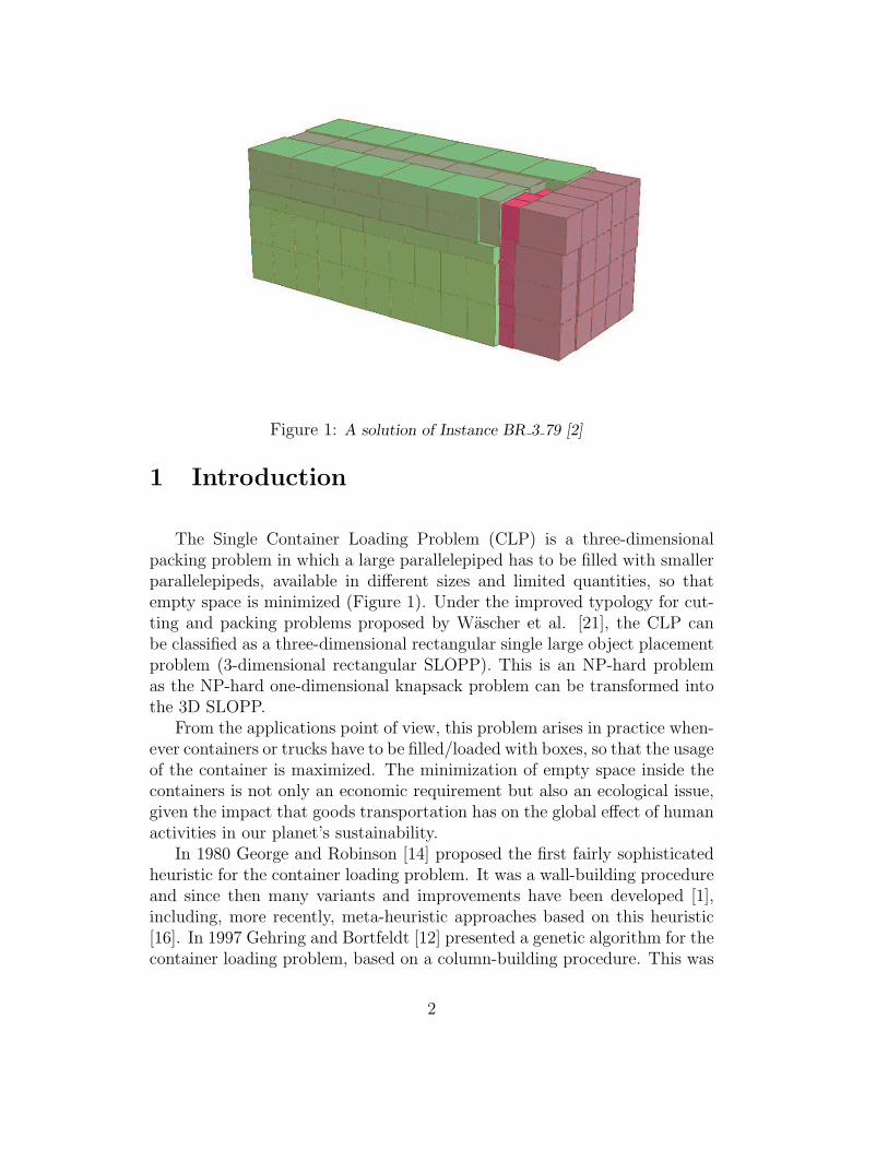
Figure 1: A solution of Instance BR 3 79 [2]

1 Introduction

The Single Container Loading Problem (CLP) is a three-dimensionalpacking problem in which a large parallelepiped has to be filled with smallerparallelepipeds, available in different sizes and limited quantities, so thatempty space is minimized (Figure 1). Under the improved typology for cut-ting and packing problems proposed by Wascher et al. [21], the CLP canbe classified as a three-dimensional rectangular single large object placementproblem (3-dimensional rectangular SLOPP). This is an NP-hard problemas the NP-hard one-dimensional knapsack problem can be transformed intothe 3D SLOPP.

From the applications point of view, this problem arises in practice when-ever containers or trucks have to be filled/loaded with boxes, so that the usageof the container is maximized. The minimization of empty space inside thecontainers is not only an economic requirement but also an ecological issue,given the impact that goods transportation has on the global effect of humanactivities in our planet’s sustainability.

In 1980 George and Robinson [14] proposed the first fairly sophisticatedheuristic for the container loading problem. It was a wall-building procedureand since then many variants and improvements have been developed [1],including, more recently, meta-heuristic approaches based on this heuristic[16]. In 1997 Gehring and Bortfeldt [12] presented a genetic algorithm for thecontainer loading problem, based on a column-building procedure. This was

2

the first of an important series of papers by those same authors who, between1998 and 2002, presented a Tabu Search [5], a hybrid Genetic Algorithm [6]and a parallel version of the genetic algorithm [13]. In the same line of work,Bortfeldt, Gehring and Mack developed a parallel tabu search algorithm[7] and a parallel hybrid local search algorithm which combines simulatedannealing and tabu search, their best algorithm so far [15]. Eley [10] pro-poses an algorithm that combines a greedy heuristic, which generates blocksof boxes, with a tree-search procedure. Moura and Oliveira [16] develop aGRASP algorithm based on a modified version of George and Robinson [14]constructive algorithm. All the previously mentioned papers have in commonthe use of a set of 1500 problems, distributed over 15 classes with differentcharacteristics as benchmark problems for the computational experiments.These problems were generated by Bischoff and Ratcliff [2]. Pisinger [17]presents a wall-building heuristic, which seems to perform quite well, butunfortunately the author does not use Bischoff and Ratcliff’s problems forhis computational experiments.

When speaking about real-world container loading problems space usageis the most important objective, but other issues have to be taken into ac-count, such as cargo stability, multi-drop loads or weight distribution ([2], [4],[8], [20]). Among these additional considerations, cargo stability is the mostimportant one. Sometimes it is explicitly taken into account in the designof the algorithms and in the definition of feasible solutions for the containerloading problem. At other times the algorithms’ results are also evaluatedagainst standard measures of cargo stability. However, when container vol-ume usage is very high, stability almost becomes a consequence of this highcargo compactness. Some freight companies value space utilization so highlythat they use foam pieces to fill the remaining gaps and increase stabilitywithout compromising space usage.

In this paper we present a new algorithm for the container loading prob-lem that is based on an original heuristic enhanced by a GRASP solu-tion space search strategy. At the core of this approach is the concept ofmaximal-spaces that explains the efficiency of the algorithm. When con-sidering Bischoff and Ratcliff’s problems, this new algorithm outperformsthe previously published approaches, taking much less computational time,mainly in the harder classes of problems.

The remainder of this paper is organized as follows: in the next sectionthe basic constructive algorithm, based on the concept of maximal-space, ispresented in its several variants. In Section 3 the GRASP implementationis presented in its constitutive parts, and in Section 4 thorough computa-tional experiments are described and results presented. Finally, in Section 5conclusions are drawn.

3

2 A constructive algorithm

At the base of any GRASP algorithm is a constructive heuristic algorithm.The constructive algorithm proposed in this paper is a block heuristic. Thebox blocks may take the shape of columns or layers. A layer is a rectangulararrangement of boxes of the same type, in rows and columns, filling one sideof the empty space. Other authors have used the term wall to refer to thesame concept. We prefer the more general term layer because it can be putvertically or horizontally in the empty space. As usual in block heuristics,the feasible placement positions are described as lists of empty spaces andeach time a block is placed in an empty space, new spaces are generated.The present block algorithm differs from the existing approaches because itrepresents the feasible placement points as a set of non-disjoint empty spaces,the maximal-spaces. This representation brings additional complexity tospace management procedures but induces increased flexibility and qualityin container loading problem solutions. Additionally, this heuristic starts toplace boxes from the eight corners of the selected empty space, according towell-defined selection criteria. Details on this new constructive heuristic aregiven in the rest of this section .

We follow an iterative process in which we combine two elements: a listB of types of boxes still to be packed, initially the complete list of boxes,and a list L of empty maximal-spaces, initially containing only the containerC. At each step, a maximal-space is chosen from L and, from the boxes inB fitting into it, a type of box and a configuration of boxes of this type arechosen to be packed. That usually produces new maximal-spaces going intoL and the process goes on until L = ∅ or none of the remaining boxes fit intoone of the remaining maximal-spaces.

• Step 0: Initialization

L={C}, the set of empty maximal-spaces.B = {b1, b2, . . . , bm}, the set of types of boxes still to be packed.qi = ni (number of boxes of type i to be packed).P = ∅, the set of boxes already packed.

• Step 1: Choosing the maximal-space in L

We have a list L of empty maximal-spaces. These spaces are calledmaximal because at each step they are the largest empty parallelepipedthat can be considered for filling with rectangular boxes. We can see anexample for a 2D problem in Figure 2. Initially we have an empty rect-angle and when we cut a piece at its bottom left corner, two maximal-spaces are generated. These spaces do not have to be disjoint. In the

4

same Figure 2 we see two more steps of the filling process with themaximal-spaces generated.

Working with maximal-spaces has two main advantages. First, we donot have to decide which disjoint spaces to generate, and then we donot need to combine disjoint spaces into new ones in order to accommo-date more boxes. We represent a maximal-space by the vertices withminimum and maximum coordinates.

To choose a maximal-space, a measure of its distance to the container’scorners is used. For every two points in R3, a = (x1, y1, z1) and b =(x2, y2, z2), we define the distance d(a, b) as the vector of components|x1 − x2|, |y1 − y2| and |z1 − z2| ordered in non-decreasing order. Forinstance, if a = (3, 3, 2) and b = (0, 5, 10), d(a, b) = (2, 3, 8), resultingfrom ordering the differences 3, 2, 8 in non-decreasing order. For eachnew maximal-space, we compute the distance from every corner of thespace to the corner of the container nearest to it and keep the minimumdistance in the lexicographical order.

d(S) = min{d(a, c), a vertex of S, c vertex of container C}

For instance, if we have the maximal-space S1 = {(4, 4, 2), (6, 6, 10)}in a (10,10,10) container, the corner of S1 nearest to a corner of thecontainer is (6,6,10) and the distance to that corner is d(S1) = (0, 4, 4).At each step we take the maximal-space with the minimum distanceto a corner of the container and use the volume of the space as a tie-breaker. If we have a second maximal-space S2 = {(1, 1, 2), (4, 4, 9)},we have dist(S1) = (0, 4, 4) and dist(S2) = (1, 1, 1). From among thesespaces we would choose space S1 to be filled with boxes. At each step,the chosen space will be denoted by S∗.

The corner of the maximal-space with the lowest distance to a corner ofthe container will be the corner in which the boxes will be packed. Thereason behind that decision is to first fill the corners of the container,then its sides and finally the inner space.

• Step 2: Choosing the boxes to pack

Once a maximal-space S∗ has been chosen, we consider the types ofboxes i of B fitting into S∗ in order to choose which one to pack. Ifqi > 1, we consider the possibility of packing a column or a layer, thatis, packing several copies of the box arranged in rows and columns, suchthat the number of boxes in the block does not exceed qi. In Figures3 and 4 we can see different possibilities for packing a box type i with

5

1 2

31 4

6

5

Figure 2: Maximal-spaces in two dimensions

qi = 12. Figure 3 shows alternatives for packing a column of boxes,while in Figure 4 we consider different ways of packing a layer with thisbox type. If some rotations of the pieces are allowed, the correspondingconfigurations will be considered.

(a) Axis X (b) Axis Y (c) Axis Z

Figure 3: Three different alternatives for a column

Two criteria have been considered to select the configuration of boxes:

i The block of boxes producing the largest increase in the objectivefunction. This is a greedy criterion in which the space is filled with

6

(a) Axis XY (b) Axis YX (c) Axis XZ

(d) Axis ZX (e) Axis YZ (f) Axis ZY

Figure 4: Six different alternatives for a layer

the block producing the largest increase in the volume occupiedby boxes.

ii The block of boxes which fits best into the maximal-space. Wecompute the distance from each side of the block to each side ofthe maximal-space and order these distances in a vector in non-decreasing order. The block is chosen using again the lexicographi-cal order. We can see an example in Figure 5, in which we considerseveral alternatives for filling an empty space of (20, 20, 10). Theblock (a) completely fills the space and its distance is (0,0,0); theblock (b) completely fills one side of the space and its distance is(0,0,9); for the block (c), only its height matches the space heightand its distance is (0,2,7); finally, none of the dimensions of block(d) matches the space dimensions and its distance is (2,2,3).

For both criteria, ties are broken by choosing the configuration with theminimum number of boxes. In Section 4 we test both criteria and makea decision about which one will be used in the final implementation.

After choosing a block with ri boxes, we update P with the type i andthe number of boxes packed and set qi = qi − ri. If qi = 0, we removepiece i from the list B.

• Step 3: Updating the list L

Unless the block fits into space S∗ exactly, packing the block produces

7

(a) (0,0,0) (b) (0,0,9) (c) (0,2,7) (d) (2,2,3)

Figure 5: Best fit of the empty space

new empty maximal-spaces, which will replace S∗ in the list L. More-over, as the maximal-spaces are not disjoint, the block being packedcan intersect with other maximal-spaces which will have to be reduced.Therefore, we have to update the list L. Once the new spaces havebeen added and some of the existing ones modified, we check the listand eliminate possible inclusions. For the sake of simplicity, Figure 2illustrates this process for a two-dimensional problem. When the sec-ond box is packed in maximal-space 2, this space is eliminated fromthe list and is replaced by two new spaces 3 and 4. When the thirdpiece is packed into maximal-space 4, as it is completely filled it justdisappears, but spaces 1 and 3 are also partially filled and must bereduced, producing spaces 5 and 6.

3 GRASP Algorithm

The GRASP algorithm was developed by Feo and Resende [11] to solvehard combinatorial problems. For an updated introduction, refer to Resendeand Ribeiro [19]. GRASP is an iterative procedure combining a constructivephase and an improvement phase. In the constructive phase a solution isbuilt step by step, adding elements to a partial solution. In order to choosethe element to be added, a greedy function is computed, which is dynamicallyadapted as the partial solution is built. However, the selection of the elementis not deterministic. A randomization strategy is added to obtain differentsolutions at each iteration. The improvement phase, usually consisting of asimple local search, follows the constructive phase.

3.1 The constructive phase

In our algorithm the constructive phase corresponds to the constructivealgorithm described in Section 2, introducing a randomization procedure

8

when selecting the type of box and the configuration to pack. We considerall feasible configurations of all types of boxes fitting into S∗ and evaluatethem according to the chosen objective function (the best increase of volumeor the best fit into the space). The configuration is selected at random fromamong a restricted set of candidates composed of the best 100δ% of theblocks, where 0 ≤ δ ≤ 1 is a parameter to be determined.

It is difficult to determine the value of δ that gives the best average results.The principle of reactive GRASP, proposed for the first time by Prais andRibeiro [18], is to let the algorithm find the best value of δ in a small setof allowed values. The parameter δ is initially taken at random from a setof discrete values {0.1, . . . , 0.8, 0.9}, but after a certain number of iterations,the relative quality of the solutions obtained with each value of δ is taken intoaccount and the probability of values consistently producing better solutionsis increased. The procedure is described in Figure 6, following Delorme etal. [9]. In this figure the parameter α is fixed at 10, as in [18].

3.2 Improvement phase

Each solution built in the constructive phase is the starting point for aprocedure in which we try to improve the solution. The procedure proposedhere consists of eliminating the final k% blocks of the solution (for instance,the final 50%) and filling the empty spaces with the deterministic constructivealgorithm. At Step 2 of the constructive algorithm we again consider the twodifferent objective functions described in Section 2, the largest increase in thevolume used and the best fit into the empty maximal-space being considered.

The improvement phase is only called if the objective function value ofthe solution of the constructive phase V ≥ Vworst +0.50(Vbest−Vworst), whereVworst and Vbest correspond to the worst and best objective function valuesof solutions obtained in previous GRASP iterations.

4 Computational experiments

The above algorithm was coded in C++ and run on a Pentium Mobile at1500 MHz with 512 Mbytes of RAM. In order to assess the relative efficiencyof our algorithm we have compared it with the most recent and efficientalgorithms proposed for the container loading problem.

9

Initialization:

D = {0.1, 0.2, . . . , 0.9}, set of possible values for δ

Vbest = 0; Vworst = ∞

nδ∗ = 0, number of iterations with δ∗, ∀ δ∗ ∈ D.

Sumδ∗ = 0, sum of values of solutions obtained with δ∗.

P (δ = δ∗) = p δ∗ = 1/|D| ,∀ δ∗ ∈ D

numIter = 0

While (numIter < maxIter)

{

Choose δ∗ from D with probability p δ∗ .

nδ∗ = nδ∗ + 1

numIter = numIter + 1

Apply Constructive Phase with δ∗obtaining solution Swith objective value V

Apply Improvement Phase obtaining solution S ′ withvalue V ′

If V′

> Vbest then Vbest = V′

.

If V′

< Vworst then Vworst = V′

Sumδ∗ = Sumδ∗ + V′

If mod(numIter, 500) == 0 :

evalδ =(

meanδ − Vworst

Vbest − Vworst

)α

∀δ ∈ D

p δ =evalδ

(

∑

δ′∈D

evalδ′

) ∀δ ∈ D

}

Figure 6: Reactive Grasp

10

4.1 Test problems

The tests were performed on 1500 problems generated by Bischoff and Ratcliff[2] and Davies and Bischoff [8]. The 1500 instances are organized into 15classes of 100 instances each. The number of box types increases from 3 inBR1 to 100 in BR15. Therefore, this set covers a wide range of situations,from weakly heterogenous to strongly heterogenous problems. The number ofboxes of each type decreases from an average of 50.2 boxes per type in BR1 toonly 1.30 in BR15. The total volume of the boxes is on average 99.46% of thecapacity of the container, but as the boxes’ dimensions have been generatedindependently of the container’s dimensions, there is no guarantee that allthe boxes of one instance can actually fit into the container. Therefore,this figure has to be used as an upper bound (probably quite loose) on themaximum percentage of volume which the boxes can fill.

Following the presentation of authors with whom we compare our re-sults, in the tables of this computational experiment section for each classwe present the average value of the solutions obtained on its 100 instances.

4.2 Choosing the best strategies

Table 1 compares the results obtained by the constructive algorithm of Sec-tion 2, when the block to pack is selected according to each one of the fourstrategies considered in Step 2, obtained by combining the two objectivefunctions (volume, best-fit) with the two types of configurations (columns,layers). This table, like all other tables in this section, shows the percent-ages of container volume occupied by boxes in the solution. The tables alsoshow the aggregate results for just the first seven classes, in order to comparewith authors who only use these classes in their computational experience.The results of Table 1 have been obtained on the complete set of 1500 testinstances. Therefore, they can be directly compared with other algorithms.If we compare them with the constructive and metaheuristic algorithms inTable 5, we can see that our initial simple constructive procedure can alreadycompete with these algorithms, especially for strongly heterogeneous classes.

In order to choose the best combination of configuration and objectivefunction we apply statistical analysis to the data summarized in Table 1.First, we use multivariate analysis of variance for repeated measures, con-sidering that for each instance we have the results obtained by the fourstrategies. These strategies define the intra-subject factor, while the instanceclasses define the inter-subject factor. This analysis allows us to consider sep-arately the effect of the strategies and the instance classes on the results ob-tained and also to make pairwise comparisons. As this analysis requires some

11

normality conditions, we also perform a non-parametric analysis for relatedmeasures, the Friedman test, and the Wilcoxon test for pairwise comparisons.Both types of tests show that the effect of the different algorithmic strategiesis statistically very significant (p < 0.001). The pairwise comparisons alsoshow significant differences for each pair of strategies. These conclusions areillustrated in Figure 7. The use of the criterion Best Fit for the objectivefunction produces results which are significantly worse than using an objec-tive function based on the increase in the volume occupied. With this ob-jective function, building layers is significantly better than building columns,but this difference only corresponds to the weakly heterogeneous instancesof the first classes. For strongly heterogeneous problems, with few copies ofeach box type, building layers is almost equivalent to building columns andthe results are very similar. In fact, over the 1500 instances, building layersgets better results in 833 cases, while building columns obtains better resultsin 623 and there are 44 ties. A first consequence of this analysis is that wewill use the objective function based on the increase of volume and we willbuild layers of boxes when filling empty spaces.

Columns LayersBest-fit Volume Best-fit Volume

BR1 82,36 82,14 85,33 84,34

BR2 82,22 82,93 85,15 84,57

BR3 81,96 84,53 85,40 85,92BR4 81,97 85,19 85,48 86,71BR5 82,39 85,16 85,49 86,52BR6 82,83 85,55 84,70 86,87BR7 83,08 86,16 84,75 86,31BR8 83,35 86,23 84,12 86,35BR9 83,75 86,00 83,89 86,29BR10 83,32 86,04 84,18 85,84

BR11 83,54 85,90 83,59 85,99BR12 83,52 85,69 83,94 85,82BR13 83,62 85,47 83,75 85,58BR14 83,30 85,45 83,71 85,50BR15 82,82 85,67 83,93 85,73Mean B1-B7 82,40 84,52 85,19 85,89Overall mean 82,94 85,21 84,49 85,89*The best values appear in bold

Table 1: Constructive phase: selecting the configuration

We have also tested whether the new distance defined in Step 1 of theconstructive algorithm, denoted as lexicographical distance, really is betterthan the usual Euclidean distance. Figure 8 shows the results obtained withboth distances. The statistical tests mentioned above, when applied to thesedata, show that using the new distance for selecting the space to fill producessignificantly better results that using the classical Euclidean distance (p <0.001).

12

81

82

83

84

85

86

87

1 2 3 4 5 6 7 8 9 10 11 12 13 14 15

Instance class

% V

olu

me Columns - Fit

Columns - Volume

Layers - Fit

Layers - Volume

Figure 7: Comparing objectives and strategies

In order to choose the best strategies for the GRASP algorithm, we havedone a limited computational study using only the first 10 instances of eachclass of problems and setting a limit of 5000 iterations. Hence, the results ofTables 2 and 3 cannot be compared with other algorithms.

Table 2 explores possible values for the percentage of removed blocks inthe improvement procedure. The values considered are 10%, 30%, 50%,70% and 90%, as well as a strategy consisting of choosing this value atrandom from [25%,75%]. We again use the parametric ANOVA procedureand the non-parametric Friedman test to compare these values. The pairwisecomparisons distinguish strategies removing 10% and 30% as significantlyworse than the others, but between the other four values, 50%, 70%, 90% orat random from [25%,75%], there are no significant differences. Therefore,we choose the value 50% because it requires less computational effort andtherefore less computing time.

The good results obtained when removing high percentages of the blocksmay seem strange at first sight. One explanation could be that the quality ofthe solutions depends critically on the layout of the first boxes packed. Therandomized constructive phase provides a wide set of alternatives for thesefirst packing steps. For the remaining boxes, at each iteration we have twoalternatives: the one obtained by continuing with the randomized procedureand the one obtained by completing the solution in a deterministic way. Theoverall results show a significant improvement when the two alternatives arecombined.

Finally, in Table 3 we compare three different improvement methods,differing in the objective function used when filling the container again with

13

81

82

83

84

85

86

87

1 2 3 4 5 6 7 8 9 10 11 12 13 14 15

Instance class

% V

olum

e

Euclidean

Lexicographic

Figure 8: Comparing distances for selecting the space to fill

the deterministic algorithm. The first one uses volume, the second the best-fitcriterion and the third uses both criteria, repeating the procedure twice. Thestatistical tests show that there are very significant differences between them,but the main reason for that result is the relatively poor performance of thebest-fit criterion, as can be seen in Figure 9. If we eliminate this alternativeand compare the other two strategies, the differences are not clear. TheWilcoxon test gives a p−value of 0.039. This is mainly due to the fact that inclasses 7 to 15 both strategies produce very similar results. However, Figure9 shows and the tests confirm that for classes 1 to 6 there is a significantdifference in favor of the strategy using both criteria. As the increase inrunning time is not too large and we are looking for an algorithm workingwell for all classes, we decided to use this strategy in the final implementation.

4.3 Studying the random component of the algorithm

The GRASP algorithm has a random component in the constructive phase.In the experiments in the previous subsection each instance was run onlyonce, but in order to assess the effect of the associated randomness, we runthe algorithm 10 times for each of the first 10 instances of each class, witha limit of 5000 iterations per run. The results are summarized in Table 4.The second column shows the results when running the algorithm just once.Columns 3 to 6 show the results for 5 runs and columns 7 to 8 the resultsof 10 runs. Finally, column 10 shows the results obtained by running thealgorithm only once, but with a limit of 50000 iterations.

The ranges of variation between the best and the worst solutions obtained

14

Removing PiecesProblem 10% 30% 50% 70% 90% Random 25%-75%BR1 92,55 92,36 92,65 92,63 92,27 92,64

BR2 93,11 93,42 93,44 93,38 93,25 93,44BR3 92,88 93,05 93,32 93,25 93,10 93,33BR4 92,60 92,91 92,87 92,91 92,56 93,00BR5 92,31 92,52 92,64 92,51 92,11 92,41

BR6 91,76 92,11 92,44 92,49 91,85 92,37

BR7 91,12 91,34 91,59 91,73 91,38 91,46

BR8 89,69 90,21 90,83 91,09 90,86 91,05

BR9 88,97 89,76 90,42 90,63 90,66 90,33

BR10 88,36 89,16 89,79 89,78 90,19 89,84

BR11 88,02 88,44 89,34 89,69 89,66 89,31

BR12 87,15 88,12 88,85 89,13 89,24 88,95

BR13 86,72 87,67 88,15 88,25 88,91 88,31

BR14 86,82 87,62 88,36 88,45 88,71 88,21

BR15 86,85 87,89 88,25 88,55 88,75 88,29

Mean B1-B7 92,33 92,53 92,71 92,70 92,36 92,67

Overall mean 89,93 90,44 90,86 90,96 90,90 90,86

*The best values appear in bold

Table 2: Percentage of removed pieces

Without Objective function for the improvement methodimproving Volume Best-fit Volume+Best-fit

Problem Vol.(%) Vol.(%) Time Vol.(%) Time Vol.(%) TimeBR1 92,09 92,65 0,88 92,84 1,04 92,95 1,11

BR2 92,86 93,46 1,85 93,79 2,17 93,95 2,39

BR3 92,24 93,32 3,50 93,21 3,87 93,54 4,39

BR4 91,95 92,87 5,06 93,21 5,63 93,05 6,53

BR5 91,36 92,59 6,43 93,02 7,09 93,01 8,21

BR6 91,11 92,41 9,40 92,20 10,42 92,72 12,14

BR7 90,13 91,58 14,51 91,34 15,99 91,62 18,80

BR8 89,20 90,87 29,65 90,39 32,35 90,74 38,69

BR9 88,08 90,42 45,74 89,61 50,16 90,43 60,44

BR10 87,31 89,79 71,20 89,02 77,54 89,69 95,94

BR11 86,83 89,37 98,60 88,64 107,33 89,29 135,12

BR12 86,72 88,95 134,79 88,09 147,07 88,95 182,96

BR13 86,16 88,15 176,94 87,91 194,19 88,22 240,71

BR14 85,99 88,36 230,60 87,34 253,25 88,25 326,26

BR15 86,26 88,30 284,83 87,33 311,56 88,30 387,41

Mean B1-B7 91,68 92,70 5,95 92,80 6,60 92,98 7,88

Overall mean 89,22 90,87 74,27 90,53 81,31 90,98 99,75

*The best values appear in bold

Table 3: Results of improvement methods

15

87

88

89

90

91

92

93

94

1 2 3 4 5 6 7 8 9 10 11 12 13 14 15

Instance class

% V

olum

e Volume

Best_Fit

Volume+Best_Fit

Figure 9: Comparing improvement methods

when running the algorithm 5 or 10 times can be obtained by subtractingcolumns 2 and 3, and columns 5 and 6. The average range for 5 runs is 0.80%and for 10 runs is 1.06%. Even with this iteration limit of 5000 iterations,the algorithm is very stable. If the iteration limit is increased, this variationis lower still.

Table 4 also indicates, and the statistical tests confirm, that if we choosethe average of the occupied volume as the measure for showing the per-formance of the algorithms, the average volumes obtained by running thealgorithm once do not differ significantly from those obtained if we run thealgorithm five or ten times and then calculate the averages of those five orten results (columns 5 and 9).

Obviously, running the algorithm 10 times and keeping the best solutionproduces better results than running it just once, but the interesting questionis whether this extra computing effort of running the algorithm 10 indepen-dent times would not be better used by running it once with a limit of 50000iterations. If the GRASP iterations were independent, the results should bethe same. In our implementation, the iterations are linked by the ReactiveGRASP procedure in which the probabilities of the values of parameter δare updated after a given number of iterations. The results of the previousiterations should guide this procedure to favor values of δ producing bestsolutions. Therefore, the results obtained using the algorithm once up to50000 iterations should be at least equal to and possibly better than thoseobtained by running it 10 independent times. The results of Table 4 showa slight advantage of the algorithm with 50000 iterations, but the statisti-cal tests performed on the results summarized in columns 6 and 10 do not

16

1 run 5 runs 10 runs 1 run5000 iter 5000 iter 5000 iter 50000 iter

Min Max Mean Min Max Mean

BR1 92.95 92.40 93.11 92.71 92.29 93.41 92.82 93.42

BR2 93.95 93.68 94.22 94.00 93,51 94.28 93.95 94.28

BR3 93.54 93.08 94.04 93.58 92.97 94.10 93.46 94.05

BR4 93.05 92.71 93.61 93.25 92.62 93.82 93.26 94.03

BR5 93.01 92.59 93.48 93.00 92,57 93.68 93.06 93.79

BR6 92.72 92.32 93.21 92.72 92,12 93.31 92.66 93.21

BR7 91.62 91.32 92.23 91.70 91,24 92.51 91.74 92.55

BR8 90.74 90.38 91.37 90.81 90.33 91.71 90.87 91.66

BR9 90.43 90.11 90.89 90.45 90.03 91.05 90.45 91.12

BR10 89.69 89.38 90.12 89.70 89.30 90.21 89.72 90.50

BR11 89.29 89.05 89.85 89.36 88.93 90.01 89.37 90.02

BR12 88.95 88.57 89.35 88.95 88.47 89.61 88.95 89.43

BR13 88.22 87.99 88.77 88.34 87.89 88.82 88.28 88.79

BR14 88.25 87.94 88.66 88.24 87.86 88.73 88.21 88.77

BR15 88.23 88.08 88.66 88.33 88.04 88.79 88.35 88.89

Mean BR1-BR7 92.98 92.59 93.41 92.99 92.48 93.59 92.99 93.62

Mean BR1-BR15 90.98 90.64 91.44 91.01 90.54 91.60 91.01 91.63

Table 4: Studying the algorithm’s randomness

show any significant difference between them. Therefore, we can draw twoconclusions. First, instead of running the algorithm 10 times and reportingthe best results obtained, we can run it once with 50000 iterations. Second,the learning mechanism of the Reactive GRASP does not seem to have anysignificant effect on the long term quality of the solutions. The preliminaryexperiments we ran showed that this way of determining δ performed betterthan other alternatives, but its effect seems to diminish in the long run.

4.4 Comparison with other algorithms

As a consequence of the results obtained in the exploratory experiments de-scribed in previous subsections, for the following computational tests theconstructive phase of the GRASP will use the lexicographical distance atStep 1, building layers of boxes at Step 2 and an objective function based onthe increase of volume. The value of the parameter δ in the randomizationprocedure will be determined by the Reactive GRASP strategy. In the im-provement phase, the final 50% of the blocks will be removed and the emptyspace filled twice, once with each objective function.

The way in which our algorithm packs the boxes, starting by packing fromthe corners, then the sides and finally the center of the container, does notguarantee cargo stability and does not produce a workable packing sequence.Therefore, a postprocessing phase in which the solution is compacted is ab-solutely necessary. We have developed a compacting procedure which takeseach box from bottom to top and tries to move it down, along axis Z, until it

17

is totally or partially supported by another box. Then, a similar proceduretakes boxes from the end to the front of the container and tries to movethem to the end, along axis Y . Finally, there is a procedure moving themfrom left to right, along axis X. The three procedures are called iterativelywhile there are boxes which have been moved. When the compacting phaseis finished, the empty spaces are checked for the possibility of packing someof the unpacked boxes. In the final solution every box is supported totallyor partially by other boxes and the boxes are given in an order in which theycan really be packed into the container.

The complete computational results on the whole set of 1500 instancesappear in Tables 5 and 6. These two tables include a direct comparisonwith the results of the best algorithms proposed in the literature, which havebenchmarked themselves against these test problems. Therefore, we compareour algorithm against 16 approaches. Among them we can distinguish twotypes of algorithms: algorithms that pack the boxes so that they are com-pletely supported by other boxes; and algorithms that do not consider thisconstraint. In the first group we have the following algorithms:

• H BR: a constructive algorithm by Bischoff and Ratcliff [2];

• H B al: a constructive algorithm by Bischoff, Janetz and Ratcliff [3];

• H B: a heuristic approach by Bischoff [4];

• GA GB: a genetic algorithm by Gehring and Bortfeldt [12];

• TS BG: a tabu search approach by Bortfeldt and Gehring [5];

• H E: a greedy constructive algorithm with an improvement phase byEley [10];

• G M: a GRASP approach by Moura and Oliveira [16].

In the second group we have the following algorithms:

• HGA BG: a hybrid genetic algorithm by Gehring and Bortfeldt [6];

• PGA GB: a parallel genetic algorithm by Gehring and Bortfeldt [13];

• PTSA: a parallel tabu search algorithm by Bortfeldt, Gehring andMack [7];

• TSA: a tabu search algorithm by Bortfeldt, Gehring and Mack [7];

18

• SA: a simulated annealing algorithm by Mack, Bortfeldt and Gehring[15];

• HYB: a hybrid algorithm by Mack, Bortfeldt and Gehring [15];

• PSA: a parallel simulated annealing algorithm by Mack, Bortfeldt andGehring [15];

• PHYB: a parallel hybrid algorithm by Mack, Bortfeldt and Gehring[15];

• PHYB XL: a massive parallel hybrid algorithm by Mack, Bortfeldtand Gehring [15];

In Table 5 we compare our GRASP algorithm (5000 iterations) withfast constructive procedures and metaheuristic algorithms requiring mod-erate computing times. The computing times cannot be compared directlybecause each author has used a different computer. In general, the run-ning times for all approaches are lower for the weakly heterogenous problemsand increase with the number of different box types. The times required byalgorithms H B al [3] and H BR [2] are not reported, but obviously thesealgorithms are very fast. H B [4] was run on a Pentium IV at 1.7 GHz, withtimes ranging on average from 26.4 seconds for BR1 to 321 seconds for BR15.H E [10] ran on a Pentium at 200 Mhz with a time limit of 600 seconds whichwas reached only for 26 out of the 700 instances of BR1-BR7. AlgorithmsGA GB, TS GB and HGA GB were run on a Pentium at 400 Mhz, withaverage times of 12, 242 and 316 seconds respectively. The parallel PGA ranon five Pentiums at 400 Mhz and took on average 183 seconds. Finally, G Mwas run on a Pentium IV at 2.4 GHz, with an average time of 69 seconds.

We can compare the fast constructive algorithms H B al and H BR withour constructive algorithm, whose results appear in the last column of Table1, using a t-test. We have tested for each class whether the average volumeobtained by our algorithm is significantly better than the reported averagesof H B al and H BR. The statistical tests conclude that for each class ourconstructive algorithm outperforms both procedures, except for class BR1,for which our results do not differ significantly from those obtained by H BR(p = 0.12).

The other algorithms in Table 5 have been compared with our GRASPalgorithm. Again, we have compared the average results obtained with ouralgorithm on the 100 instances of each class with the averages reported foreach class by the other algorithms. The statistical tests confirm that ourGRASP algorithm gets significantly better results for every class. The dif-ferences are more important for strongly heterogeneous problems. In fact,

19

as Bortfeldt et al. state in their papers, their algorithms are best suited forweakly heterogeneous classes. In particular, their Tabu Search algorithm,TS BG, obtains very good results in relatively short times in the first sevenclasses. In any case, the Bortfeldt et al. algorithms will be more adequatelycompared in Table 6, where their more recent and powerful procedures areconsidered.

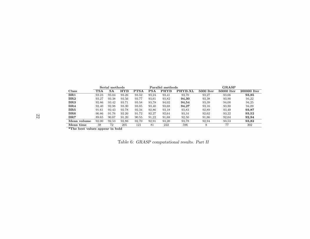
Table 6 compares GRASP with more recent metaheuristics that requirelonger computing times, especially in their parallel versions. In this case,we have allowed our algorithm to run up to an extremely high number ofiterations, 200000, to assess its performance for longer running times. Thelast row of the table shows the reported average running times. They are in-cluded only as a reference, because the algorithms have been run on differentcomputers. Mack et al. [15] use a Pentium-PC at 2Ghz for the serial pro-cedures, a LAN of four of these computers for the parallel implementationof PSA and PHYB and a LAN of sixty-four computers for the PHYB.XLimplementation.

An approximate comparison, according to the reported running times,would be to compare our version of the GRASP algorithm with 50000 it-erations with the serial methods and GRASP with 200000 iterations withthe parallel methods. In the first set of comparisons, we compare the bestserial method, HYB, with our GRASP with 50000 iterations. The statisticaltests show that our algorithm outperforms the serial methods for all classes,except for BR1 in which the p − value is 0.052 and the equality cannot berejected at a level α = 0.05. In a second series of comparisons, we com-pare the best results of the three parallel methods, PTSA, PSA and PHYBwith our GRASP with 200000 iterations. Again, our algorithm produces sig-nificantly better results for all classes (p < 0.01), except for BR1 in whichthe p − value is 0.114. Finally, we compare the massively parallel methodPHYB.XL with GRASP with 200000 iterations. In this case, equality cannotbe rejected for classes BR1, BR2 and BR5 (with p− values of 0.48, 0,52 and0.66), PHYB.XL is better for classes BR3 and BR4 and GRASP is better forclasses BR6 and BR7. Again, the Mack et al. algorithms work very well forweakly heterogeneous classes but our procedure obtains progressively betterresults when heterogeneity increases.

5 Conclusions

We have developed a new GRASP algorithm which obtains good results forall classes of test instances, from weakly to strongly heterogeneous problems,especially for the latter. We think that these good results are due to three

20

Problem class H B al H BR GA GB TS BG HGA BG PGA GB H B H E G M GRASP TimeBR1 81,76 83,37 86,77 92,63 87,81 88,1 89,39 88 89,07 93,27 1,27

BR2 81,7 83,57 88,12 92,7 89,4 89,56 90,26 88,5 90,43 93,38 2,32

BR3 82,98 83,59 88,87 92,31 90,48 90,77 91,08 89,5 90,86 93,39 4,62

BR4 82,6 84,16 88,68 91,62 90,63 91,03 90,9 89,3 90,42 93,16 6,52

BR5 82,76 83,89 88,78 90,86 90,73 91,23 91,05 89 89,57 92,89 8,58

BR6 81,5 82,92 88,53 90,04 90,72 91,28 90,7 89,2 89,71 92,62 12,23

BR7 80,51 82,14 88,36 88,63 90,65 91,04 90,44 88 88,05 91,86 19,25

BR8 79,65 80,1 87,52 87,11 89,73 90,26 — — 86,13 91,02 38,20

BR9 80,19 78,03 86,46 85,76 89,06 89,5 — — 85,08 90,46 63,10

BR10 79,74 76,53 85,53 84,73 88,4 88,73 — — 84,21 89,87 97,08

BR11 79,23 75,08 84,82 83,55 87,53 87,87 — — 83,98 89,36 136,50

BR12 79,16 74,37 84,25 82,79 86,94 87,18 — — 83,64 89,03 183,21

BR13 78,23 73,56 83,67 82,29 86,25 86,7 — — 83,54 88,56 239,80

BR14 77,4 73,37 82,99 81,33 85,55 85,81 — — 83,25 88,46 307,62

BR15 75,15 73,38 82,47 80,85 85,23 85,48 — — 83,21 88,36 394,66

Mean B1-B7 81,97 83,38 88,30 91,26 90,06 90,43 90,55 88,79 89,73 92,94 7,83

Mean 80,17 79,2 86,39 87,15 88,61 88,97 — — 86,74 91,05 101,00

*The best values appear in bold

Table 5: GRASP computational results. Part I

21

Serial methods Parallel methods GRASPClass TSA SA HYB PTSA PSA PHYB PHYB.XL 5000 Iter 50000 Iter 200000 IterBR1 93.23 93.04 93.26 93.52 93,24 93,41 93,70 93,27 93,66 93,85BR2 93.27 93.38 93.56 93.77 93,61 93,82 94,30 93,38 93,90 94,22

BR3 92.86 93.42 93.71 93.58 93,78 94,02 94,54 93,39 94,00 94,25

BR4 92.40 92.98 93.30 93.05 93,40 93,68 94,27 93,16 93,80 94,09

BR5 91.61 92.43 92.78 92.34 92,86 93,18 93,83 92,89 93,49 93,87BR6 90.86 91.76 92.20 91.72 92,27 92,64 93,34 92,62 93,22 93,52BR7 89.65 90.67 91.20 90.55 91,22 91,68 92,50 91,86 92,64 92,94Mean volume 92.00 92,53 92,86 92,70 92,91 93,20 93,78 92,94 93,53 93,82Mean time 38 72 205 121 81 222 596 8 77 302

*The best values appear in bold

Table 6: GRASP computational results. Part II

22

main reasons. First, the use of maximal-spaces allows us to have, at eachstep, the best possible spaces into which a box can fit. Second, the way inwhich the spaces are filled, though it seems counterintuitive, keeps maximalempty spaces larger and available for packing new boxes. Third, the GRASPscheme permits the combination of randomized and deterministic packingstrategies. We have performed a preliminary computational test to deter-mine the best strategies and parameter values from among those we havedesigned. The resulting algorithm produces good quality solutions in shortcomputing times and can improve them if longer times are available. Byadding a post processing phase in which the solutions are compacted, theybecome more stable and are sometimes even improved in terms of volumeutilization. Nevertheless, more complex metaheuristics, based on the sameideas but adding more powerful improvement schemes, could improve theresults further. The next phase of our research will address this aspect.

Acknowledgements

This study has been partially supported by the Spanish Ministry of Sci-ence and Technology, DPI2005-04796, and by Project PBI-05-022, Consejeriade Ciencia y Tecnologia, Junta de Comunidades de Castilla-La Mancha.

We also thank professor Ana Moura, from the Polytechnic Institute ofLeiria, Portugal, for the fruitful discussions on this work.

References

[1] Bischoff, E.E. and Marriot, M.D. (1990) A Comparative Evalu-ation of Heuristics for Container Loading, European Journal of Opera-

tional Research, 44, 267-276.

[2] Bischoff, E.E. and Ratcliff, M.S.W. (1995) Issues in the Devel-opment of Approaches to Container Loading, Omega, 23, 377–390.

[3] Bischoff, E.E. Janetz, F. and Ratcliff, M.S.W. (1995) Load-ing Pallets with Nonidentical Items, European Journal of Operational

Research, 84, 681–692.

[4] Bischoff, E.E. (2006) Three dimensional packing of items with lim-ited load bearing strength, European Journal of Operational Research,168, 952–966.

23

[5] Bortfeldt, A. and Gehring, H. (1998) A Tabu Search Algorithmfor Weakly Heterogeneous Container Loading Problems, OR Spectrum,20, 237–250.

[6] Bortfeldt, A. and Gehring, H. (2001) A Hybrid Genetic Algo-rithm for the Container Loading Problem, European Journal of Opera-

tional Research, 131, 143–161.

[7] Bortfeldt, A. Gehring, H. and Mack, D. (2003) A Parallel TabuSearch Algorithm for Solving the Container Loading Problem, Parallel

Computing 29, 641–662.

[8] Davies, A.P. and Bischoff, E.E. (1998) Weight distribution consid-erations in container loading. Working Paper, European Business Man-agement School, Statistics and OR Group, University of Wales, Swansea.

[9] Delorme, X. and Gandibleux, X. and Rodriguez, J. (2003)GRASP for set packing problems, European Journal of Operational Re-

search 153, 564-580.

[10] Eley, M. (2002) Solving Container Loading Problems by Block Ar-rangement, European Journal of Operational Research, 141, 393–409.

[11] Feo, T. and Resende, M.G.C. (1989) A Probabilistic Heuristic fora Computationally Difficult Set Covering Problem, Operations Research

Letters 8, 67-71.

[12] Gehring, H. and Bortfeldt, A. (1997) A Genetic Algorithm forSolving the Container Loading Problem, International Transactions in

Operational Research, 4, 401–418.

[13] Gehring, H. and Bortfeldt, A. (2002) A Parallel Genetic Algo-rithm for Solving the Container Loading Problem, International Trans-

actions in Operational Research, 9, 497–511.

[14] George, J. A. and Robinson, D. F. (1980) A Heuristic for PackingBoxes into a Container, Computers and Operations Research, 7, 147-156.

[15] Mack, D. Bortfeldt, A. and Gehring, H. (2004) A Parallelhybrid local search algorithm for the container loading problem, Inter-

national Transactions in Operational Research 11, 511–533.

[16] Moura, A. and Oliveira, J.F. (2005) A GRASP approach to theContainer-Loading Problem IEEE Intelligent Systems, 20, 50-57.

24

[17] Pisinger, D. (2002) Heuristics for the container loading problem,European Journal of Operational Research, 141, 382-392.

[18] Prais, M. and Ribeiro, C.C. (2000) Reactive GRASP: An applica-tion to a matrix decomposition problem in TDMA traffic assignment,INFORMS Journal on Computing 12, 164-176.

[19] Resende, M.G.C and Ribeiro, C.C. (2003) Greedy RandomizedAdaptive Search Procedures, in Handbook of Metaheuristics, F.Gloverand G.Kochenberger, Eds., Kluwer Academic Publishers, pp. 219-249.

[20] Ratcliff, M. S. W. and Bischoff, E. E. (1998) Allowing for weightconsiderations in container loading, OR Spectrum, 20, 65-71.

[21] Wascher, G. and Haussner, H. and Schumann, H. An improvedtypology of cutting and packing problems, European Journal of Opera-

tional Research, in Press.

25