A lossless earth Green’s function representationbetween any two subsurface points from surface

reflection GPR dataEvert Slob and Kees Wapenaar

Department of Geoscience & Engineering, Delft University of TechnologyStevinweg 1, 2628 CN, Delft, The Netherlandse.c.slob@tudelft.nl, c.p.a.wapenaar@tudelft.nl

Abstract—We present a three-dimensional scheme that can beused to compute the electromagnetic impulse response betweenany two subsurface points from surface reflection data measuredat a single surface of a lossless medium. The scheme firstcomputes a virtual vertical radar profile using the Marchenkoscheme from which focusing wavefields are computed. With theaid of the Green’s functions of the virtual vertical radar profilesthese focusing wavefields are then used to compute the Green’sfunction between any two points in the subsurface. One point isa virtual receiver and the other point is a virtual source. Virtualradar images can be created as well as the whole time evolutionof the radar wave field in the whole subsurface generated byone virtual source. We show with a numerical example that themethod works well in a one-dimensional configuration.

Index Terms—virtual source, virtual receiver, interferometry,autofocusing, 3D GPR.

I. INTRODUCTION

Virtual receivers can be placed inside an acoustic scatteringmedium without having a physical source at the locationof the virtual receiver [1], [2]. For ground-penetrating radarthe theory for the electric and magnetic field in the earthimpulse responses at virtual subsurface receiver locations werederived in [3] assuming a lossless earth model. These Green’sfunctions of virtual vertical radar profiles can be obtained in1D without any model information and in 3D with limitedmodel information. The required information in 3D is thattravel time from a source location at the measurement surfaceto the virtual receiver location inside the scattering mediummust be estimated from the data, which requires some velocityanalysis similar to what is done for standard imaging. Forground-penetrating radar it is important to include conductivityor more general dissipation/dispersion effects, for which ageneral theory for acoustic waves and electromagnetic wavescan be found in [4], [5]. Retrieving virtual vertical radarprofiles in a dissipative medium requires access at two sideof the medium and the full scattering matrix as input data.Retrieving up- and downgoing parts of the Green’s functionfor a virtual receiver inside the earth allows for creating animage that is free from artefacts. Such artefacts would occurwhen the measured surface reflection response would be usedto make an image using a standard (model-driven) migrationscheme [6]–[8] or linearised inversion [9].

A next step is creating the Green’s functions between anytwo points in the subsurface. These are of relevance forholography, imaging, inverse scattering, and Green’s func-tion retrieval from ambient noise. A general unified theorywas developed in [10] that can be used e.g., for acoustic,electromagnetic, and elastic wavefield applications. Here wederive the electromagnetic Green’s function representationfor a virtual source and a virtual receiver both located inthe subsurface. We show how these virtual earth impulseresponses can be obtained form the measured reflection re-sponse on the earth surface in a multi-source, multi-receiveracquisition configuration. We restrict ourselves to losslessmedia to be able to work with the surface reflection re-sponse only. The representations are given in the frequencydomain, but are valid in the time domain. To this end, wedefine the time-Fourier transform of a space-time depen-dent vector-quantity as u(x, ω) =

∫∞t=0

exp(−jωt)u(x, t)dt,where j is the imaginary unit, ω denotes angular frequency,and x is the position vector in three-dimensional space. Inthe space-frequency domain the electromagnetic field vec-tor u is given by ut(x, ω) = (ut

1(x, ω), ut2(x, ω)) =(

(Ex, Ey)t, (Hy,−Hx)

t)

, with Ex(x, ω) and Hx(x, ω) be-ing the x-components of the electric and magnetic field vectorsand the superscript t denotes transposition. The domain D isbounded by measurement surfaces at two depth levels givenby ∂D0 at z = z0 and ∂Dm at z = zm, the focusing depthlevel ∂Di is at z = zi with z0 < zi < zm. In what followsthe physical sources are outside the domain D. Hence insideD the Maxwell equations can be written as

∂3

(u1

u2

)=

(O M1

M2 O

)(u1

u2

), (1)

with material paramater operator matrices given by

M1 =

(−ζ + ∂xη

−1∂x ∂xη−1∂y

∂yη−1∂x −ζ + ∂yη

−1∂y

), (2)

M2 =

(−η + ∂yζ

−1∂y −∂yζ−1∂x−∂xζ−1∂y −η + ∂xζ

−1∂z

), (3)

where η = jωε and ζ = jωµ. Notice that M tn = Mn and

M †n = −Mn, for n = 1, 2, and where the superscript † means

complex conjugation and transposition.

II. GREEN’S FUNCTION REPRESENTATION FOR VERTICALSOURCE AND VIRTUAL RECEIVER

At any location in between the outer depth levels of D wecan write the horizontal components of the electric field asup- and downgoing electric wavefields according to [3]

u1 = u+1 + u−1 , (4)

where u+1 denotes the downgoing and u−1 denotes the upgoing

electric field components and a similar expression can beused for the magnetic field. The horizontal components of theelectric and magnetic field vectors can be written in terms ofthe up- and downgoing magnetic and electric fields as [11]

u1 = M−12 ∂z(u

+2 + u−2 ), (5)

u2 = M−11 ∂z(u

+1 + u−1 ). (6)

Following the procedure in [3] we apply the reciprocitytheorem of the convolution and correlation types to wavefieldsin the same medium. Exploiting the separation in up- anddowngoing waves we can select to use only electric fieldmeasurements by Following a procedure similar to the onegiven in Appendix C in [12] we assume that the permeabilityand permittivity at the depth levels z0 and zi are continuouslydifferentiable in horizontal direction, then we find∫

∂D0

[(u+

2;A)tu−1;B + (u−2;A)

tu+1;B

]d2x

= −∫∂Di

[(u−1;A)

tu+2;B + (u+

1;A)tu−2;B

]d2x, (7)

and ∫∂D0

[(u+

2;A)†u+

1;B + (u+2;A)

†u+1;B

]d2x

= −∫∂Di

[(u+

1;A)†u+

2;B + (u+1;A)

†u+1;B

]d2x. (8)

In equation (8) an additional approximation is made by ignor-ing evanescent waves at depth levels z0 and zi.

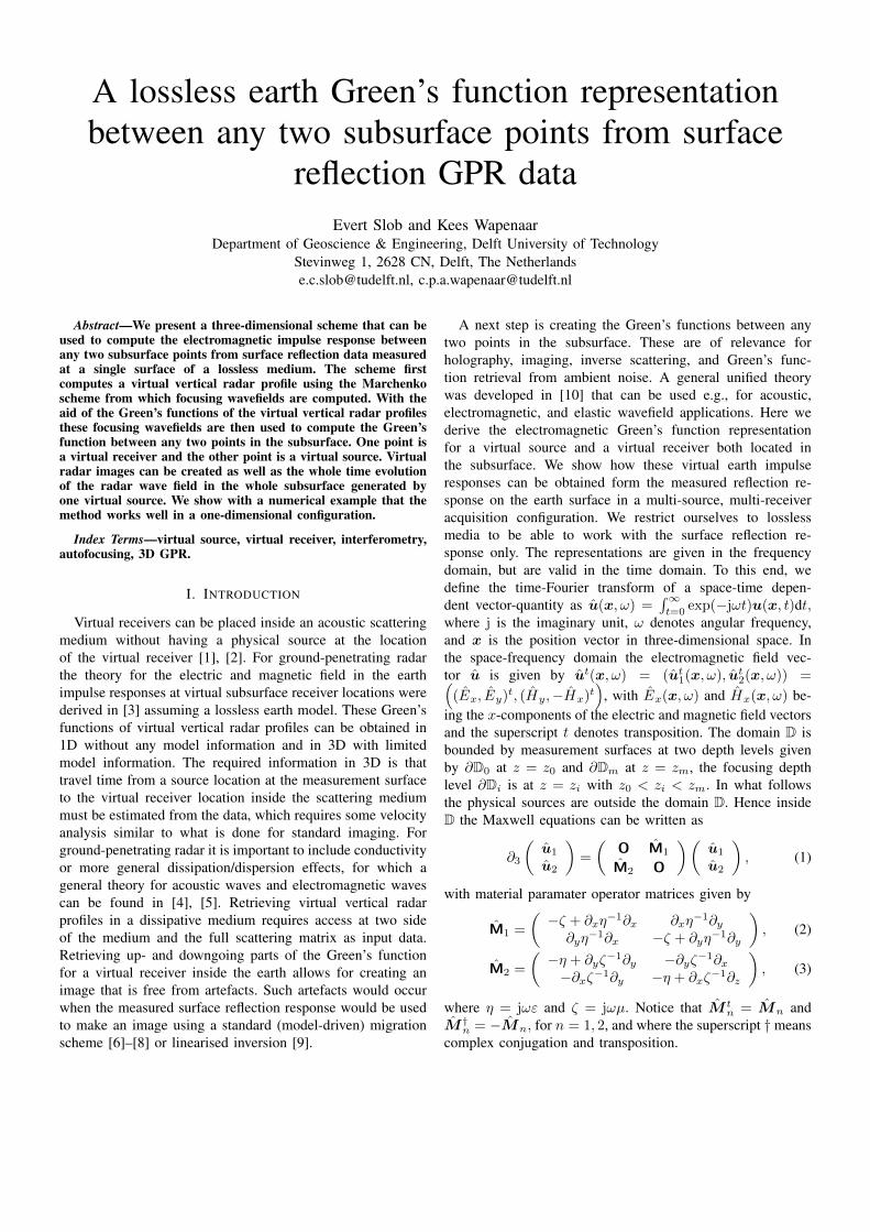
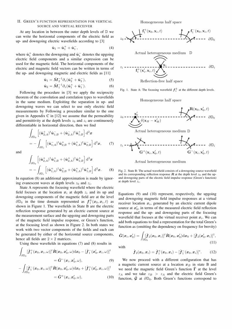
State A represents the focusing wavefield where the electricfield focuses at the location xi at depth zi and its up anddowngoing components of the magnetic field are at the level∂D0 in the time domain represented as f±1 (x0,xi, t) asshown in Figure 1. The wavefields in State B are the electricreflection response generated by an electric current source atthe measurement surface and the upgoing and downgoing partsof the magnetic field impulse response, or Green’s function,at the focusing level as shown in Figure 2. In both states wework with two vector components of the fields and each canbe generated by either of the horizontal source components,hence all fields are 2× 2 matrices.

Using these wavefields in equations (7) and (8) results in∫∂D0

[f+1 (x0,xi, ω)]

tR(x0,x′0, ω)dx0 − [f−1 (x

′0,xi, ω)]

t

= G−(xi,x′0, ω), (9)

−∫∂D0

[f−1 (x0,xi, ω)]†R(x0,x

′0, ω)dx0 + [f+

1 (x′0,xi, ω)]

†

= G+(xi,x′0, ω), (10)

@Dizi •

DActual heterogeneous medium

Reflection-free half space

f+1 (x0

i,xi, t)

Homogeneous half space

@D0z0

f+1 (x0,xi, t) f�1 (x0,xi, t)

xi

Fig. 1. State A: The focusing wavefield f±1 at the different depth levels.

Homogeneous half space

D

@Dizi

Actual heterogeneous medium

Actual heterogeneous medium

• @D0z0

R(x0,x00, t)

G+(xi,x00, t) G�(xi,x

00, t)

�(xH � x0H)

x00

Fig. 2. State B: The actual wavefield consists of a downgoing source wavefieldand its corresponding reflection response R at the depth level z0 and the up-and downgoing parts of the electric field impulse response (Green’s function)at depth level zi.

Equations (9) and (10) represent, respectively, the upgoingand downgoing magnetic field impulse responses at a virtualreceiver location xi, generated by an electric current dipolesource at x′0, in terms of the measured electric field reflectionresponse and the up- and downgoing parts of the focusingwavefield that focuses at the virtual receiver point xi. We canadd both equations to find a representation for the total Green’sfunction as (omitting the dependency on frequency for brevity)

G(xi,x′0) =

∫∂D0

[f2(x0,xi)]tR(x0,x

′0)dx0 + [f2(x

′0,xi)]

†,

(11)with

f2(x0,xi) = f+1 (x0,xi)− [f−1 (x0,xi)]

∗. (12)

We now proceed with a different configuration that hasa magnetic current source at a location xB in state B andwe need the magnetic field Green’s function Γ at the levelzA and we take zB > zA and the electric field Green’sfunction, G at ∂D0. Both Green’s functions correspond to

fields generated by a magnetic current source and hence at∂DA we have u±2;B = Γ±(xA,xB , ω) and at ∂D0 we haveu−1;B = G(x′0,xB , ω) and u+

1;B = 0. In state A we chooseagain the same focusing wavefields as before, but now thecorresponding electric field focuses at xA at ∂DA. Substitutingthese choices in equations (7) and (8) gives

Γ−(xA,xB) =

∫∂D0

[f+1 (x

′0,xA)]

tG(x′0,xB)dx′0, (13)

Γ+(xA,xB) = −∫∂D0

[f−1 (x′0,xA)]

†G(x′0,xB)dx′0. (14)

We can add these equations, transpose both sides anduse source-receiver reciprocity for both Green’s functions([Γ(xA,xB)]

t = Γ(xB ,xA), G(x′0,xB) = −[G(xB ,x′0)]

t)to find the final Green’s function representation

Γ(xB ,xA) = −∫∂D0

G(xB ,x′0)f2(x

′0,xA)dx

′0. (15)

These equations are valid when zA < zB . When zA > zB wemust first put the magnetic source in state B at xA and focusat xB and obtain

[Γ(xB ,xA)]t = −

∫∂D0

G(xA,x′0)f2(x

′0,xB)dx

′0. (16)

Starting with the electric field reflection response measured,and generated by an electric dipole source, at the surface ofa lossless medium we first use the magnetic field focusingwavefield to bring the receivers into the subsurface after whichwe use the same focusing wavefield to bring the sources intothe subsurface. In this process we end up with the magneticfield response at any subsurface location xA generated by amagnetic dipole at any subsurface location xB . To carry outthese two steps we need to obtain the focusing wavefields f±1and the procedure is described in detail in [3] and not repeatedhere. We suffice to say that equations (9) and (10) must besolved in the time domain in the interval where the Green’sfunctions are zero. Once these are found equations (12) and(11) are used to compute the Green’s functions G, whichare then used in equations (15) and (16) to compute theGreen’s fucntions between any two locations in the subsurface.These can be useful in many applications including monitoringapplications.

III. NUMERICAL EXAMPLE

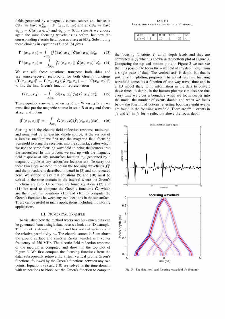
To visualise how the method works and how much data canbe generated from a single data trace we look at a 1D example.The model is shown in Table I and has vertical variations inthe relative permittivity εr. The electric source is 5 cm abovethe ground surface and emits a Ricker wavelet with centerfrequency of 250 MHz. The electric field reflection responseof the medium is computed and shown in the top plot ofFigure 3. We first compute the focusing functions from thedata, subsequently retrieve the virtual vertical profile Green’sfunctions, followed by the Green’s functions between any twopoints. Equations (9) and (10) are solved in the time domainwith truncations to block out the Green’s function to compute

TABLE ILAYER THICKNESS AND PERMITTIVITY MODEL.

d (m) 0.05 0.60 1.75 1 ∞εr(−) 1 16 4 25 4

the focusing functions f1 at all depth levels and they arecombined in f2 which is shown in the bottom plot of Figure 3.Comparing the top and bottom plots in Figure 3 we can seethat it is possible to focus the wavefield at any depth level froma single trace of data. The vertical axis is depth, but that isjust done for plotting purposes. The actual resulting focusingwavefield comes as a function of one-way travel time and ina 1D model there is no information in the data to convertthose times to depth. In the bottom plot we can also see thatevery time we cross a boundary when we focus deeper intothe model the number of events double and when we focusbelow the fourth and bottom reflecting boundary eight eventsare found in the focusing wavefield. There are 2n−1 events inf1 and 2n in f2 for n reflectors above the focus depth.

time (ns)0 50 100 150

str

ength

(V

/m)

-100

-50

0

50

100

150

200

250electric field from electric dipole

focusing wavefield

time (ns)-50 0 50

focus d

epth

(m

)

0

0.5

1

1.5

2

2.5

3

3.5

Fig. 3. The data (top) and focusing wavefield f2 (bottom).

magnetic field from electric dipole

time (ns)0 20 40 60 80 100

depth

(m

)0

0.5

1

1.5

2

2.5

3

3.5

magnetic field from magnetic dipole

time (ns)0 10 20 30 40 50 60 70

depth

(m

)

0

0.5

1

1.5

2

2.5

3

3.5

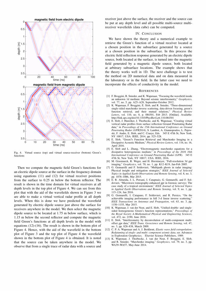
Fig. 4. Virtual source (top) and virtual source-receiver (bottom) Green’sfunctions

Then we compute the magnetic field Green’s functions foran electric dipole source at the surface in the frequency domainusing equations (11) and (12) for virtual receiver positionsfrom the surface to 0.25 m below the bottom reflector. Theresult is shown in the time domain for virtual receivers at alldepth levels in the top plot of Figure 4. We can see from thisplot that with the aid of the wavefields shown in Figure 3 weare able to make a virtual vertical radar profile at all depthlevels. When this is done we have predicted the wavefieldgenerated by electric dipole source just above the surface forreceivers anywhere in the model. We then select the magneticdipole source to be located at 1.75 m below surface, which is1.15 m below the second reflector and compute the magneticfield Green’s functions at all depth levels in the model withequations (12)-(16). The result is shown in the bottom plot ofFigure 4. Hence, with the aid of the wavefield in the bottomplot of Figure 3 and the top plot of Figure 4 the wavefieldshown in the bottom plot of Figure 4 is obtained. It is notedthat the source can be taken anywhere in the model. Weobserve that from a single trace of radar data with a source and

receiver just above the surface, the receiver and the source canbe put at any depth level and all possible multi-source multi-receiver wavefields (data cube) can be computed.

IV. CONCLUSION

We have shown the theory and a numerical example toretrieve the Green’s function of a virtual receiver located ata chosen position in the subsurface generated by a sourceat a chosen position in the subsurface. In this process theelectric field reflection response generated by an electric dipolesource, both located at the surface, is turned into the magneticfield generated by a magnetic dipole source, both locatedat arbitrary subsurface locations. The example shows thatthe theory works well in 1D. The next challenge is to testthe method on 2D numerical data and on data measured inthe laboratory or in the field. In the latter case we need toincorporate the effects of conductivity in the model.

REFERENCES

[1] F. Broggini, R. Snieder, and K. Wapenaar, “Focusing the wavefield insidean unknown 1d medium: Beyond seismic interferometry,” Geophysics,vol. 77, no. 5, pp. A25–A28, September-October 2012.

[2] K. Wapenaar, F. Broggini, E. Slob, and R. Snieder, “Three-dimensionalsingle-sided marchenko inverse scattering, data-driven focusing, green’sfunction retrieval, and their mutual relations,” Physical ReviewLetters, vol. 110, no. 8, p. 084301, Feb 2013. [Online]. Available:http://link.aps.org/doi/10.1103/PhysRevLett.110.084301

[3] E. Slob, J. Hunziker, J. Thorbecke, and K. Wapenaar, “Creating virtualvertical radar profiles from surface reflection Ground Penetrating Radardata,” in Proceedings of the 15th International Conference on GroundPenetrating Radar (GPR2014), S. Lambot, A. Giannopoulos, L. Pajew-ski, F. Andre, E. Slob, and C. Craeye, Eds. 345 E 47th St, New York,NY 10017, USA: IEEE, 2014, pp. 525–528.

[4] E. Slob, “Green?s Function Retrieval and Marchenko Imaging in aDissipative Acoustic Medium,” Physical Review Letters, vol. 116, no. 16,April 2016.

[5] E. Slob and L. Zhang, “Electromagnetic marchenko equations for adissipative heterogeneous medium,” in Proceedings of the 2016 16thInternational Conference on Ground Penetrating Radar (GPR). 345 E47th St, New York, NY 10017, USA: IEEE, 2016.

[6] M. Grasmueck, R. Weger, and H. Horstmeyer, “Full-resolution 3d gprimaging,” Geophysics, vol. 70, no. 1, pp. K12–K19, Jan-Feb 2005.

[7] G. Gennarelli and F. Soldovieri, “Multipath ghosts in radar imaging:Physical insight and mitigation strategies,” IEEE Journal of SelectedTopics in Applied Earth Observations and Remote Sensing, vol. 8, no. 3,pp. 1078–1086, Mar 2015.

[8] E. R. Almeida, J. L. Porsani, I. Catapnaio, G. Gennarelli, and F. Sol-dovieri, “Microwave tomography-enhanced gpr in forensic surveys: Thecase study of a tropical environment,” IEEE Journal of Selected Topicsin Applied Earth Observations and Remote Sensing, vol. 9, no. 1, pp.115–124, Jan 2016.

[9] G. Gennarelli, I. Catapano, F. Soldovieri, and R. Persico, “On theachievable imaging performance in full 3-d linear inverse scattering,”IEEE Transactions on Antennas and Propagation, vol. 63, no. 3, pp.1150–1155, Mar 2015.

[10] K. Wapenaar, J. van der Neut, and E. Slob, “Unified double- and single-sided homogeneous Green’s function representations,” Proceedings ofthe Royal Society A-Mathematical Physical and Engineering Sciences,vol. 472, no. 2190, June 2016.

[11] E. Slob, “Interferometry by deconvolution of multi-component multi-offset gpr data,” IEEE Trans. Geoscience and Remote Sensing, vol. 47,no. 3, pp. 828–838, March 2009.

[12] C. P. A. Wapenaar and A. J. Berkhout, Elastic wave field extrapolation:Redatuming of single- and multi- component seismic data, ser. Advancesin Exploration Geophysics. Elsevier Science Publishers, 1989.

[13] K. Wapenaar, J. Thorbecke, J. van der Neut, F. Broggini, E. Slob,and R. Snieder, “Marchenko imaging,” Geophysics, vol. 79, no. 3, pp.WA39–WA57, May-June 2014.