a laplacian framework for option discovery in ... · a laplacian framework for option discovery in...

A Laplacian Framework for Option Discovery in Reinforcement Learning

Marlos C. Machado 1 Marc G. Bellemare 2 Michael Bowling 1

AbstractRepresentation learning and option discovery aretwo of the biggest challenges in reinforcementlearning (RL). Proto-value functions (PVFs) area well-known approach for representation learn-ing in MDPs. In this paper we address the op-tion discovery problem by showing how PVFsimplicitly define options. We do it by introduc-ing eigenpurposes, intrinsic reward functions de-rived from the learned representations. The op-tions discovered from eigenpurposes traverse theprincipal directions of the state space. They areuseful for multiple tasks because they are discov-ered without taking the environment’s rewardsinto consideration. Moreover, different optionsact at different time scales, making them help-ful for exploration. We demonstrate features ofeigenpurposes in traditional tabular domains aswell as in Atari 2600 games.

1. IntroductionTwo important challenges in reinforcement learning (RL)are the problems of representation learning and of auto-matic discovery of skills. Proto-value functions (PVFs)are a well-known solution for the problem of representa-tion learning (Mahadevan, 2005; Mahadevan & Maggioni,2007); while the problem of skill discovery is generallyposed under the options framework (Sutton et al., 1999;Precup, 2000), which models skills as options.

In this paper, we tie together representation learning andoption discovery by showing how PVFs implicitly defineoptions. One of our main contributions is to introducethe concepts of eigenpurpose and eigenbehavior. Eigen-purposes are intrinsic reward functions that incentivize theagent to traverse the state space by following the principaldirections of the learned representation. Each intrinsic re-ward function leads to a different eigenbehavior, which isthe optimal policy for that reward function. In this paper we

1University of Alberta 2Google DeepMind. Correspondenceto: Marlos C. Machado <[email protected]>.

Appearing in the Proceedings of the 34 th International Confer-ence on Machine Learning, Sydney, Australia, PMLR 70, 2017.

introduce an algorithm for option discovery that leveragesthese ideas. The options we discover are task-independentbecause, as PVFs, the eigenpurposes are obtained withoutany information about the environment’s reward structure.We first present these ideas in the tabular case and thenshow how they can be generalized to the function approxi-mation case.

Exploration, while traditionally a separate problem fromoption discovery, can also be addressed through the carefulconstruction of options (McGovern & Barto, 2001; Simseket al., 2005; Solway et al., 2014; Kulkarni et al., 2016).In this paper, we provide evidence that not all options ca-pable of accelerating planning are useful for exploration.We show that options traditionally used in the literature tospeed up planning hinder the agents’ performance if usedfor random exploration during learning. Our options havetwo important properties that allow them to improve explo-ration: (i) they operate at different time scales, and (ii) theycan be easily sequenced. Having options that operate atdifferent time scales allows agents to make finely timed ac-tions while also decreasing the likelihood the agent will ex-plore only a small portion of the state space. Moreover, be-cause our options are defined across the whole state space,multiple options are available in every state, which allowsthem to be easily sequenced.

2. BackgroundWe generally indicate random variables by capital letters(e.g.,Rt), vectors by bold letters (e.g., θ), functions by low-ercase letters (e.g., v), and sets by calligraphic font (e.g., S).

2.1. Reinforcement Learning

In the RL framework (Sutton & Barto, 1998), an agent aimsto maximize cumulative reward by taking actions in an en-vironment. These actions affect the agent’s next state andthe rewards it experiences. We use the MDP formalismthroughout this paper. An MDP is a 5-tuple 〈S,A, r, p, γ〉.At time t the agent is in state st ∈ S where it takes actionat ∈ A that leads to the next state st+1 ∈ S according tothe transition probability kernel p(s′|s, a), which encodesPr(St+1 = s′|St = s,At = a). The agent also observesa reward Rt+1 ∼ r(s, a). The agent’s goal is to learn apolicy µ : S × A → [0, 1] that maximizes the expected

arX

iv:1

703.

0095

6v2

[cs

.LG

] 1

6 Ju

n 20

17


discounted returnGt.= Ep,µ

[∑∞k=0 γ

kRt+k+1|st], where

γ ∈ [0, 1) is the discount factor.

It is common to use the policy improvement theorem (Bell-man, 1957) when learning to maximize Gt. One techniqueis to alternate between solving the Bellman equations forthe action-value function qµk

(s, a),

qµk(s, a)

.= Eµk,p

[Gt|St = s,At = a

]=∑s′,r

p(s′, r|s, a)[r + γ

∑a′

µk(a′|s′)qµk(s′, a′)

]and making the next policy, µk+1, greedy w.r.t. qµk

,

µk+1.= arg max

a∈Aqµk

(s, a),

until converging to an optimal policy µ∗.

Sometimes it is not feasible to learn a value for each state-action pair due to the size of the state space. Generally,this is addressed by parameterizing qµ(s, a) with a set ofweights θ ∈ Rn such that qµ(s, a) ≈ qµ(s, a,θ). It iscommon to approximate qµ through a linear function, i.e.,qµ(s, a,θ) = θ>φ(s, a), where φ(s, a) denotes a linearfeature representation of state s when taking action a.

2.2. The Options Framework

The options framework extends RL by introducing tempo-rally extended actions called skills or options. An option ωis a 3-tuple ω = 〈I, π, T 〉 where I ∈ S denotes the op-tion’s initiation set, π : A×S→ [0, 1] denotes the option’spolicy, and T ∈ S denotes the option’s termination set. Af-ter the agent decides to follow option ω from a state in I,actions are selected according to π until the agent reaches astate in T . Intuitively, options are higher-level actions thatextend over several time steps, generalizing MDPs to semi-Markov decision processes (SMDPs) (Puterman, 1994).

Traditionally, options capable of moving agents to bottle-neck states are sought after. Bottleneck states are thosestates that connect different densely connected regions ofthe state space (e.g., doorways) (Simsek & Barto, 2004;Solway et al., 2014). They have been shown to be veryefficient for planning as these states are the states most fre-quently visited when considering the shortest distance be-tween any two states in an MDP (Solway et al., 2014).

2.3. Proto-Value Functions

Proto-value functions (PVFs) are learned representationsthat capture large-scale temporal properties of an environ-ment (Mahadevan, 2005; Mahadevan & Maggioni, 2007).They are obtained by diagonalizing a diffusion model,which is constructed from the MDP’s transition matrix. Adiffusion model captures information flow on a graph, and

it is commonly defined by the combinatorial graph Lapla-cian matrix L = D − A, where A is the graph’s adja-cency matrix and D the diagonal matrix whose entries arethe row sums of A. Notice that the adjacency matrix Aeasily generalizes to a weight matrix W . PVFs are de-fined to be the eigenvectors obtained after the eigendecom-position of L. Different diffusion models can be used togenerate PVFs, such as the normalized graph LaplacianL = D−

12 (D −A)D−

12 , which we use in this paper.

3. Option Discovery through the LaplacianPVFs capture the large-scale geometry of the environment,such as symmetries and bottlenecks. They are task inde-pendent, in the sense that they do not use information re-lated to reward functions. Moreover, they are defined overthe whole state space since each eigenvector induces a real-valued mapping over each state. We can imagine that op-tions with these properties should also be useful. In thissection we show how to use PVFs to discover options.

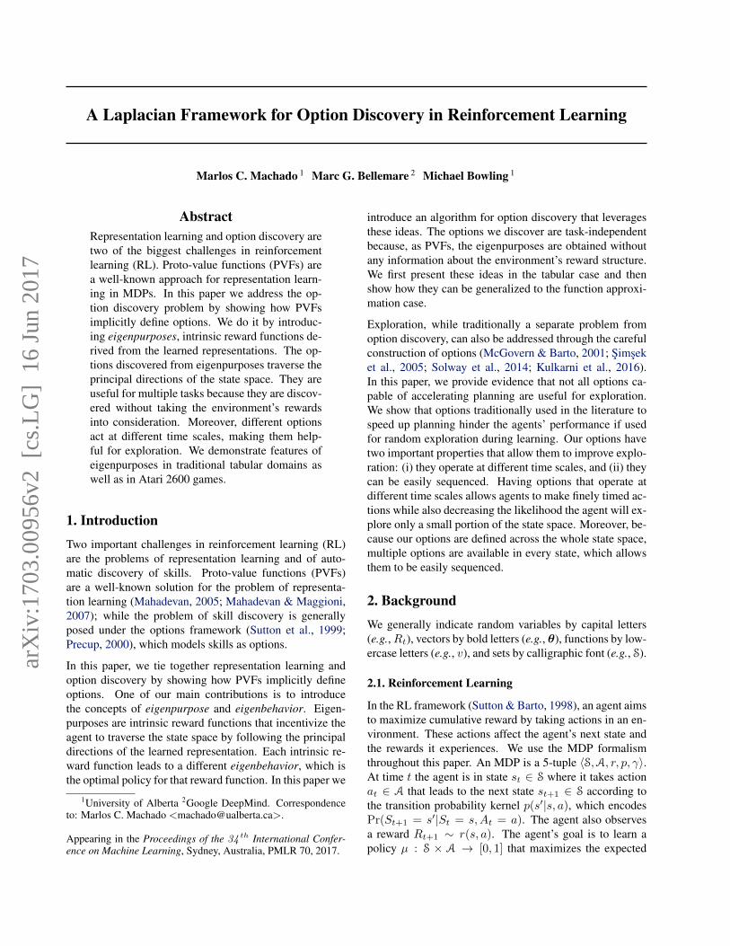
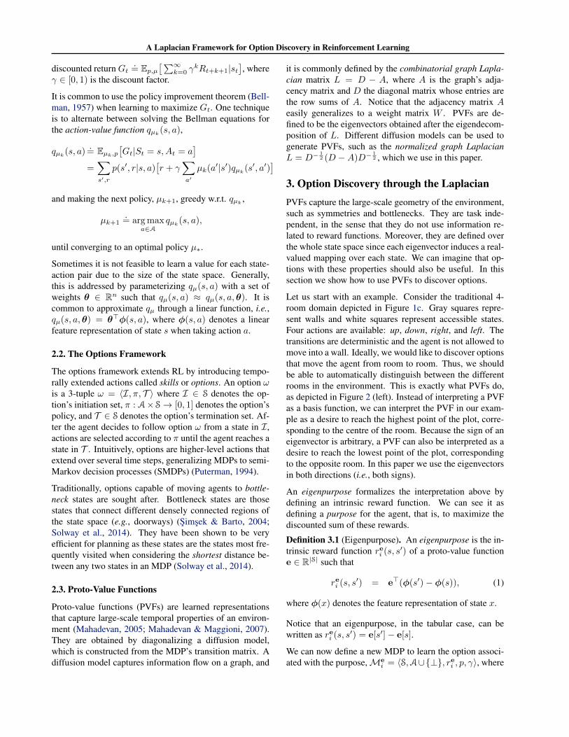
Let us start with an example. Consider the traditional 4-room domain depicted in Figure 1c. Gray squares repre-sent walls and white squares represent accessible states.Four actions are available: up, down, right, and left. Thetransitions are deterministic and the agent is not allowed tomove into a wall. Ideally, we would like to discover optionsthat move the agent from room to room. Thus, we shouldbe able to automatically distinguish between the differentrooms in the environment. This is exactly what PVFs do,as depicted in Figure 2 (left). Instead of interpreting a PVFas a basis function, we can interpret the PVF in our exam-ple as a desire to reach the highest point of the plot, corre-sponding to the centre of the room. Because the sign of aneigenvector is arbitrary, a PVF can also be interpreted as adesire to reach the lowest point of the plot, correspondingto the opposite room. In this paper we use the eigenvectorsin both directions (i.e., both signs).

An eigenpurpose formalizes the interpretation above bydefining an intrinsic reward function. We can see it asdefining a purpose for the agent, that is, to maximize thediscounted sum of these rewards.

Definition 3.1 (Eigenpurpose). An eigenpurpose is the in-trinsic reward function rei (s, s′) of a proto-value functione ∈ R|S| such that

rei (s, s′) = e>(φ(s′)− φ(s)), (1)

where φ(x) denotes the feature representation of state x.

Notice that an eigenpurpose, in the tabular case, can bewritten as rei (s, s′) = e[s′]− e[s].

We can now define a new MDP to learn the option associ-ated with the purpose,Me

i = 〈S,A∪{⊥}, rei , p, γ〉, where


(a) 10×10 grid (b) I-Maze (c) 4-room domain

Figure 1. Domains used for evaluation.

the reward function is defined as in (1) and the action set isaugmented by the action terminate (⊥), which allows theagent to leave Me

i without any cost. The state space andthe transition probability kernel remain unchanged from theoriginal problem. The discount rate can be chosen arbitrar-ily, although it impacts the timescale the option encodes.

With Mei we define a new state-value function veπ(s), for

policy π, as the expected value of the cumulative dis-counted intrinsic reward if the agent starts in state s andfollows policy π until termination. Similarly, we define anew action-value function qeπ(s, a) as the expected valueof the cumulative discounted intrinsic reward if the agentstarts in state s, takes action a, and then follows policy πuntil termination. We can also describe the optimal valuefunction for any eigenpurpose obtained through e:

ve∗(s) = maxπ

veπ(s) and qe∗(s, a) = maxπ

qeπ(s, a).

These definitions naturally lead us to eigenbehaviors.

Definition 3.2 (Eigenbehavior). An eigenbehavior is a pol-icy χe : S → A that is optimal with respect to the eigen-purpose rei , i.e., χe(s) = arg maxa∈A q

e∗(s, a).

Finding the optimal policy πe∗ now becomes a traditional

RL problem, with a different reward function. Importantly,this reward function tends to be dense, avoiding challeng-ing situations due to exploration issues. In this paper weuse policy iteration to solve for an optimal policy.

If each eigenpurpose defines an option, its correspondingeigenbehavior is the option’s policy. Thus, we need to de-fine the option’s initiation and termination set. An optionshould be available in every state where it is possible toachieve its purpose, and to terminate when it is achieved.

When defining the MDP to learn the option, we augmentedthe agent’s action set with the terminate action, allowingthe agent to interrupt the option anytime. We want optionsto terminate when the agent achieves its purpose, i.e., whenit is unable to accumulate further positive intrinsic rewards.With the defined reward function, this happens when theagent reaches the state with largest value in the eigenpur-pose (or a local maximum when γ < 1). Any subsequentreward will be negative. We are able to formalize this con-

Figure 2. Second PVF (left) and its corresponding option (right)in the 4-room domain. Action terminate is depicted in red (topright corner), other actions are depicted as arrows.

dition by defining qχ(s,⊥).= 0 for all χe. When the ter-

minate action is selected, control is returned to the higherlevel policy (Dietterich, 2000). An option following a pol-icy χe terminates when qeχ(s, a) ≤ 0 for all a ∈ A. Wedefine the initiation set to be all states in which there existsan action a ∈ A such that qeχ(s, a) > 0. Thus, the option’spolicy is πe(s) = arg maxa∈A∪{⊥} q

eπ(s, a). We refer to

the options discovered with our approach as eigenoptions.The eigenoption corresponding to the example at the be-ginning of this section is depicted in Figure 2 (right).

For any eigenoption, there is always at least one state inwhich it terminates, as we now show.

Theorem 3.1 (Option’s Termination). Consider aneigenoption o = 〈Io, πo, To〉 and γ < 1. Then, in anMDP with finite state space, To is nonempty.

Proof. We can write the Bellman equation in the matrixform: v = r+γTv, where v is a finite column vector withone entry per state encoding its value function. From (1)we have r = Tw−w with w = φ(s)>e, where e denotesthe eigenpurpose of interest. Therefore:

v + w = Tw + γTv

= (1− γ)Tw + γT (v + w)

= (1− γ)(I − γT )−1Tw.

||v + w||∞ = (1− γ)||(I − γT )−1Tw||∞||v + w||∞ ≤ (1− γ)||(I − γT )−1T ||∞||w||∞

||v + w||∞ ≤ (1− γ)1

(1− γ)||w||∞

||v + w||∞ ≤ ||w||∞

We can shift w by any finite constant without changing thereward, i.e., Tw−w = T (w+δ)−(w+δ) because T1δ =1δ since

∑j Ti,j = 1. Hence, we can assume w≥ 0. Let

s∗ = arg maxsws∗ , so that ws∗ = ||w||∞. Clearly vs∗ ≤0, otherwise ||v + w||∞ ≥ |vs∗ + ws∗ | = vs∗ + ws∗ >ws∗ = ||w||∞, arriving at a contradiction.


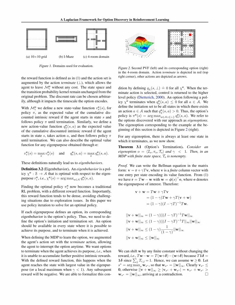
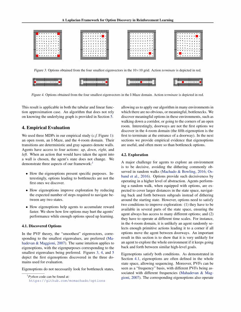
Figure 3. Options obtained from the four smallest eigenvectors in the 10×10 grid. Action terminate is depicted in red.

Figure 4. Options obtained from the four smallest eigenvectors in the I-Maze domain. Action terminate is depicted in red.

This result is applicable in both the tabular and linear func-tion approximation case. An algorithm that does not relyon knowing the underlying graph is provided in Section 5.

4. Empirical EvaluationWe used three MDPs in our empirical study (c.f. Figure 1):an open room, an I-Maze, and the 4-room domain. Theirtransitions are deterministic and gray squares denote walls.Agents have access to four actions: up, down, right, andleft. When an action that would have taken the agent intoa wall is chosen, the agent’s state does not change. Wedemonstrate three aspects of our framework:1

• How the eigenoptions present specific purposes. In-terestingly, options leading to bottlenecks are not thefirst ones we discover.

• How eigenoptions improve exploration by reducingthe expected number of steps required to navigate be-tween any two states.

• How eigenoptions help agents to accumulate rewardfaster. We show how few options may hurt the agents’performance while enough options speed up learning.

4.1. Discovered Options

In the PVF theory, the “smoothest” eigenvectors, corre-sponding to the smallest eigenvalues, are preferred (Ma-hadevan & Maggioni, 2007). The same intuition applies toeigenoptions, with the eigenpurposes corresponding to thesmallest eigenvalues being preferred. Figures 3, 4, and 5depict the first eigenoptions discovered in the three do-mains used for evaluation.

Eigenoptions do not necessarily look for bottleneck states,

1Python code can be found at:https://github.com/mcmachado/options

allowing us to apply our algorithm in many environments inwhich there are no obvious, or meaningful, bottlenecks. Wediscover meaningful options in these environments, such aswalking down a corridor, or going to the corners of an openroom. Interestingly, doorways are not the first options wediscover in the 4-room domain (the fifth eigenoption is thefirst to terminate at the entrance of a doorway). In the nextsections we provide empirical evidence that eigenoptionsare useful, and often more so than bottleneck options.

4.2. Exploration

A major challenge for agents to explore an environmentis to be decisive, avoiding the dithering commonly ob-served in random walks (Machado & Bowling, 2016; Os-band et al., 2016). Options provide such decisiveness byoperating in a higher level of abstraction. Agents perform-ing a random walk, when equipped with options, are ex-pected to cover larger distances in the state space, navigat-ing back and forth between subgoals instead of ditheringaround the starting state. However, options need to satisfytwo conditions to improve exploration: (1) they have to beavailable in several parts of the state space, ensuring theagent always has access to many different options; and (2)they have to operate at different time scales. For instance,in the 4-room domain, it is unlikely an agent randomly se-lects enough primitive actions leading it to a corner if alloptions move the agent between doorways. An importantresult in this section is to show that it is very unlikely foran agent to explore the whole environment if it keeps goingback and forth between similar high-level goals.

Eigenoptions satisfy both conditions. As demonstrated inSection 4.1, eigenoptions are often defined in the wholestate space, allowing sequencing. Moreover, PVFs can beseen as a “frequency” basis, with different PVFs being as-sociated with different frequencies (Mahadevan & Mag-gioni, 2007). The corresponding eigenoptions also operate

https://github.com/mcmachado/options


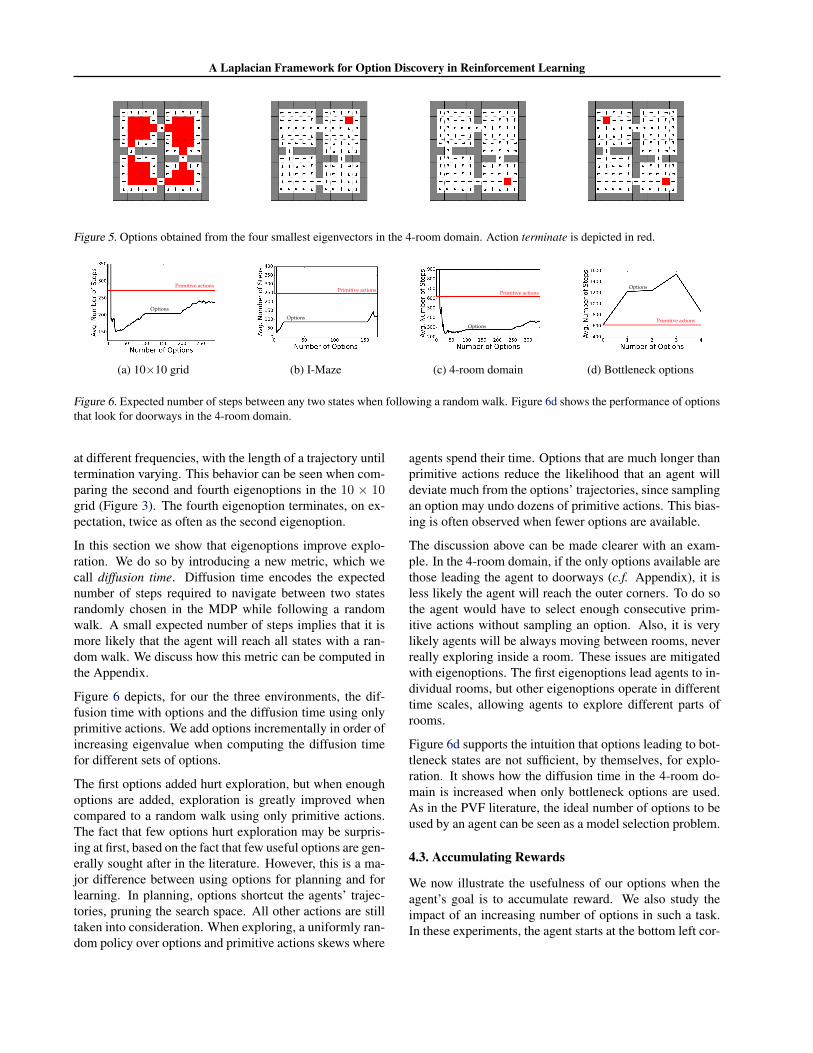
Figure 5. Options obtained from the four smallest eigenvectors in the 4-room domain. Action terminate is depicted in red.

Primitive actions

Options

(a) 10×10 grid

Primitive actions

Options

(b) I-Maze

Primitive actions

Options

(c) 4-room domain

Primitive actions

Options

(d) Bottleneck options

Figure 6. Expected number of steps between any two states when following a random walk. Figure 6d shows the performance of optionsthat look for doorways in the 4-room domain.

at different frequencies, with the length of a trajectory untiltermination varying. This behavior can be seen when com-paring the second and fourth eigenoptions in the 10 × 10grid (Figure 3). The fourth eigenoption terminates, on ex-pectation, twice as often as the second eigenoption.

In this section we show that eigenoptions improve explo-ration. We do so by introducing a new metric, which wecall diffusion time. Diffusion time encodes the expectednumber of steps required to navigate between two statesrandomly chosen in the MDP while following a randomwalk. A small expected number of steps implies that it ismore likely that the agent will reach all states with a ran-dom walk. We discuss how this metric can be computed inthe Appendix.

Figure 6 depicts, for our the three environments, the dif-fusion time with options and the diffusion time using onlyprimitive actions. We add options incrementally in order ofincreasing eigenvalue when computing the diffusion timefor different sets of options.

The first options added hurt exploration, but when enoughoptions are added, exploration is greatly improved whencompared to a random walk using only primitive actions.The fact that few options hurt exploration may be surpris-ing at first, based on the fact that few useful options are gen-erally sought after in the literature. However, this is a ma-jor difference between using options for planning and forlearning. In planning, options shortcut the agents’ trajec-tories, pruning the search space. All other actions are stilltaken into consideration. When exploring, a uniformly ran-dom policy over options and primitive actions skews where

agents spend their time. Options that are much longer thanprimitive actions reduce the likelihood that an agent willdeviate much from the options’ trajectories, since samplingan option may undo dozens of primitive actions. This bias-ing is often observed when fewer options are available.

The discussion above can be made clearer with an exam-ple. In the 4-room domain, if the only options available arethose leading the agent to doorways (c.f. Appendix), it isless likely the agent will reach the outer corners. To do sothe agent would have to select enough consecutive prim-itive actions without sampling an option. Also, it is verylikely agents will be always moving between rooms, neverreally exploring inside a room. These issues are mitigatedwith eigenoptions. The first eigenoptions lead agents to in-dividual rooms, but other eigenoptions operate in differenttime scales, allowing agents to explore different parts ofrooms.

Figure 6d supports the intuition that options leading to bot-tleneck states are not sufficient, by themselves, for explo-ration. It shows how the diffusion time in the 4-room do-main is increased when only bottleneck options are used.As in the PVF literature, the ideal number of options to beused by an agent can be seen as a model selection problem.

4.3. Accumulating Rewards

We now illustrate the usefulness of our options when theagent’s goal is to accumulate reward. We also study theimpact of an increasing number of options in such a task.In these experiments, the agent starts at the bottom left cor-


Primitiveactions

2 options

4 options

8 options

64 options128 options256 options

(a) 10×10 grid

Primitiveactions

2 options

4 options

8 options

64 options 128 options

(b) I-Maze

Primitiveactions

2 options

4 options

8 options

64 options 128 options256 options

(c) 4-room domain

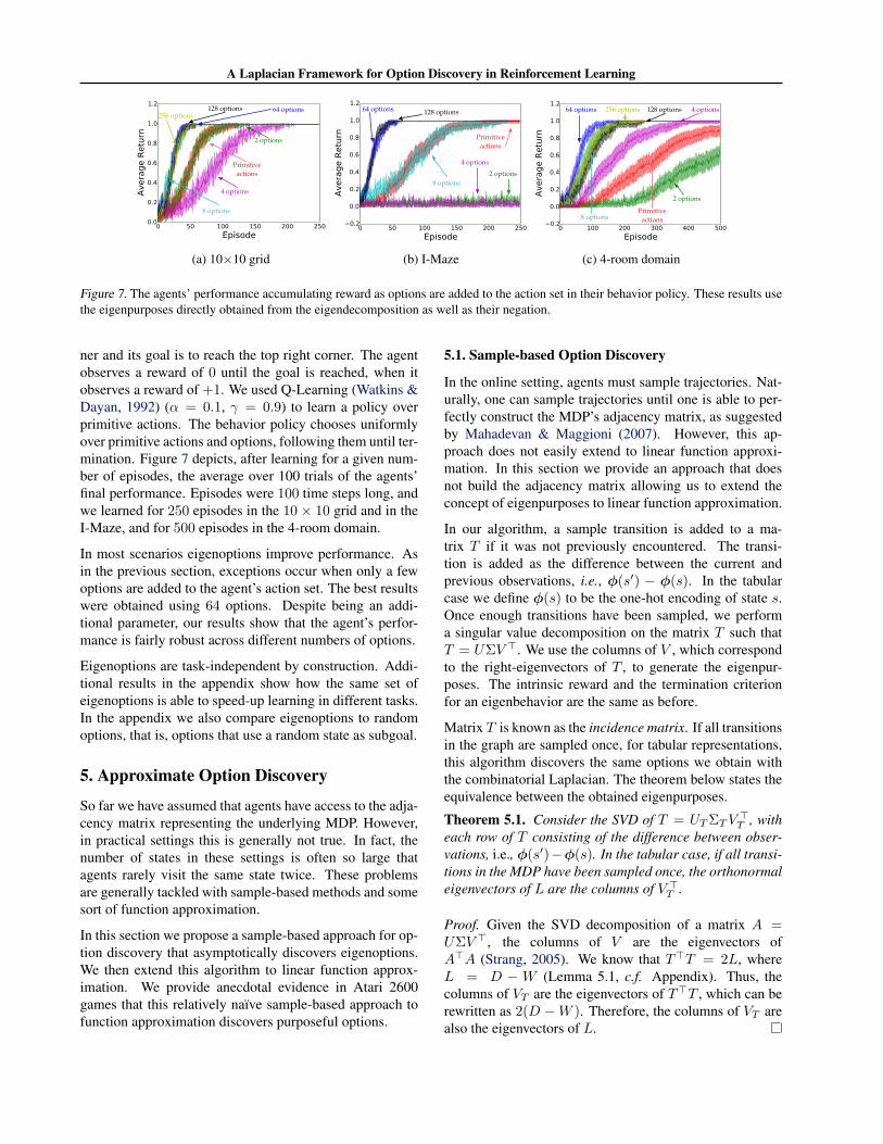
Figure 7. The agents’ performance accumulating reward as options are added to the action set in their behavior policy. These results usethe eigenpurposes directly obtained from the eigendecomposition as well as their negation.

ner and its goal is to reach the top right corner. The agentobserves a reward of 0 until the goal is reached, when itobserves a reward of +1. We used Q-Learning (Watkins &Dayan, 1992) (α = 0.1, γ = 0.9) to learn a policy overprimitive actions. The behavior policy chooses uniformlyover primitive actions and options, following them until ter-mination. Figure 7 depicts, after learning for a given num-ber of episodes, the average over 100 trials of the agents’final performance. Episodes were 100 time steps long, andwe learned for 250 episodes in the 10 × 10 grid and in theI-Maze, and for 500 episodes in the 4-room domain.

In most scenarios eigenoptions improve performance. Asin the previous section, exceptions occur when only a fewoptions are added to the agent’s action set. The best resultswere obtained using 64 options. Despite being an addi-tional parameter, our results show that the agent’s perfor-mance is fairly robust across different numbers of options.

Eigenoptions are task-independent by construction. Addi-tional results in the appendix show how the same set ofeigenoptions is able to speed-up learning in different tasks.In the appendix we also compare eigenoptions to randomoptions, that is, options that use a random state as subgoal.

5. Approximate Option Discovery

So far we have assumed that agents have access to the adja-cency matrix representing the underlying MDP. However,in practical settings this is generally not true. In fact, thenumber of states in these settings is often so large thatagents rarely visit the same state twice. These problemsare generally tackled with sample-based methods and somesort of function approximation.

In this section we propose a sample-based approach for op-tion discovery that asymptotically discovers eigenoptions.We then extend this algorithm to linear function approx-imation. We provide anecdotal evidence in Atari 2600games that this relatively naıve sample-based approach tofunction approximation discovers purposeful options.

5.1. Sample-based Option Discovery

In the online setting, agents must sample trajectories. Nat-urally, one can sample trajectories until one is able to per-fectly construct the MDP’s adjacency matrix, as suggestedby Mahadevan & Maggioni (2007). However, this ap-proach does not easily extend to linear function approxi-mation. In this section we provide an approach that doesnot build the adjacency matrix allowing us to extend theconcept of eigenpurposes to linear function approximation.

In our algorithm, a sample transition is added to a ma-trix T if it was not previously encountered. The transi-tion is added as the difference between the current andprevious observations, i.e., φ(s′) − φ(s). In the tabularcase we define φ(s) to be the one-hot encoding of state s.Once enough transitions have been sampled, we performa singular value decomposition on the matrix T such thatT = UΣV >. We use the columns of V , which correspondto the right-eigenvectors of T , to generate the eigenpur-poses. The intrinsic reward and the termination criterionfor an eigenbehavior are the same as before.

Matrix T is known as the incidence matrix. If all transitionsin the graph are sampled once, for tabular representations,this algorithm discovers the same options we obtain withthe combinatorial Laplacian. The theorem below states theequivalence between the obtained eigenpurposes.

Theorem 5.1. Consider the SVD of T = UTΣTV>T , with

each row of T consisting of the difference between obser-vations, i.e., φ(s′)−φ(s). In the tabular case, if all transi-tions in the MDP have been sampled once, the orthonormaleigenvectors of L are the columns of V >T .

Proof. Given the SVD decomposition of a matrix A =UΣV >, the columns of V are the eigenvectors ofA>A (Strang, 2005). We know that T>T = 2L, whereL = D − W (Lemma 5.1, c.f. Appendix). Thus, thecolumns of VT are the eigenvectors of T>T , which can berewritten as 2(D −W ). Therefore, the columns of VT arealso the eigenvectors of L.


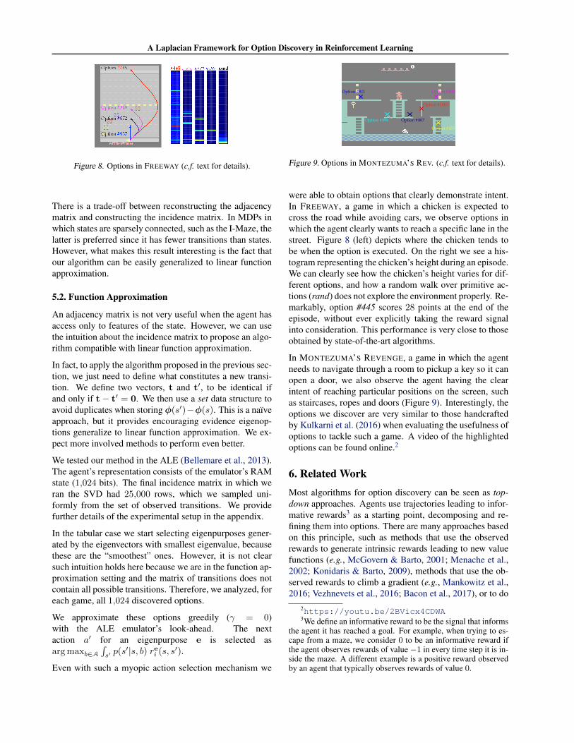
Figure 8. Options in FREEWAY (c.f. text for details).

There is a trade-off between reconstructing the adjacencymatrix and constructing the incidence matrix. In MDPs inwhich states are sparsely connected, such as the I-Maze, thelatter is preferred since it has fewer transitions than states.However, what makes this result interesting is the fact thatour algorithm can be easily generalized to linear functionapproximation.

5.2. Function Approximation

An adjacency matrix is not very useful when the agent hasaccess only to features of the state. However, we can usethe intuition about the incidence matrix to propose an algo-rithm compatible with linear function approximation.

In fact, to apply the algorithm proposed in the previous sec-tion, we just need to define what constitutes a new transi-tion. We define two vectors, t and t′, to be identical ifand only if t− t′ = 0. We then use a set data structure toavoid duplicates when storing φ(s′)−φ(s). This is a naıveapproach, but it provides encouraging evidence eigenop-tions generalize to linear function approximation. We ex-pect more involved methods to perform even better.

We tested our method in the ALE (Bellemare et al., 2013).The agent’s representation consists of the emulator’s RAMstate (1,024 bits). The final incidence matrix in which weran the SVD had 25,000 rows, which we sampled uni-formly from the set of observed transitions. We providefurther details of the experimental setup in the appendix.

In the tabular case we start selecting eigenpurposes gener-ated by the eigenvectors with smallest eigenvalue, becausethese are the “smoothest” ones. However, it is not clearsuch intuition holds here because we are in the function ap-proximation setting and the matrix of transitions does notcontain all possible transitions. Therefore, we analyzed, foreach game, all 1,024 discovered options.

We approximate these options greedily (γ = 0)with the ALE emulator’s look-ahead. The nextaction a′ for an eigenpurpose e is selected asarg maxb∈A

∫s′p(s′|s, b) rei (s, s′).

Even with such a myopic action selection mechanism we

Option #1005

Option #994 Option #807


Option #455

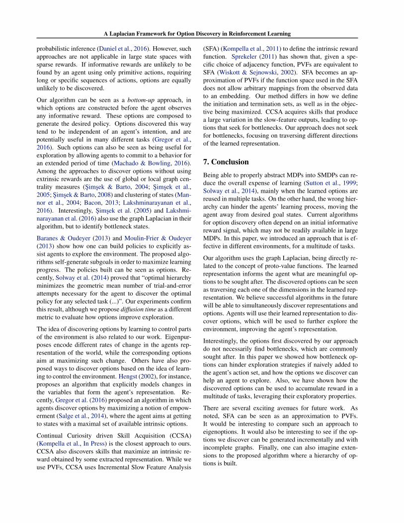
Figure 9. Options in MONTEZUMA’S REV. (c.f. text for details).

were able to obtain options that clearly demonstrate intent.In FREEWAY, a game in which a chicken is expected tocross the road while avoiding cars, we observe options inwhich the agent clearly wants to reach a specific lane in thestreet. Figure 8 (left) depicts where the chicken tends tobe when the option is executed. On the right we see a his-togram representing the chicken’s height during an episode.We can clearly see how the chicken’s height varies for dif-ferent options, and how a random walk over primitive ac-tions (rand) does not explore the environment properly. Re-markably, option #445 scores 28 points at the end of theepisode, without ever explicitly taking the reward signalinto consideration. This performance is very close to thoseobtained by state-of-the-art algorithms.

In MONTEZUMA’S REVENGE, a game in which the agentneeds to navigate through a room to pickup a key so it canopen a door, we also observe the agent having the clearintent of reaching particular positions on the screen, suchas staircases, ropes and doors (Figure 9). Interestingly, theoptions we discover are very similar to those handcraftedby Kulkarni et al. (2016) when evaluating the usefulness ofoptions to tackle such a game. A video of the highlightedoptions can be found online.2

6. Related WorkMost algorithms for option discovery can be seen as top-down approaches. Agents use trajectories leading to infor-mative rewards3 as a starting point, decomposing and re-fining them into options. There are many approaches basedon this principle, such as methods that use the observedrewards to generate intrinsic rewards leading to new valuefunctions (e.g., McGovern & Barto, 2001; Menache et al.,2002; Konidaris & Barto, 2009), methods that use the ob-served rewards to climb a gradient (e.g., Mankowitz et al.,2016; Vezhnevets et al., 2016; Bacon et al., 2017), or to do

2https://youtu.be/2BVicx4CDWA3We define an informative reward to be the signal that informs

the agent it has reached a goal. For example, when trying to es-cape from a maze, we consider 0 to be an informative reward ifthe agent observes rewards of value −1 in every time step it is in-side the maze. A different example is a positive reward observedby an agent that typically observes rewards of value 0.

https://youtu.be/2BVicx4CDWA


probabilistic inference (Daniel et al., 2016). However, suchapproaches are not applicable in large state spaces withsparse rewards. If informative rewards are unlikely to befound by an agent using only primitive actions, requiringlong or specific sequences of actions, options are equallyunlikely to be discovered.

Our algorithm can be seen as a bottom-up approach, inwhich options are constructed before the agent observesany informative reward. These options are composed togenerate the desired policy. Options discovered this waytend to be independent of an agent’s intention, and arepotentially useful in many different tasks (Gregor et al.,2016). Such options can also be seen as being useful forexploration by allowing agents to commit to a behavior foran extended period of time (Machado & Bowling, 2016).Among the approaches to discover options without usingextrinsic rewards are the use of global or local graph cen-trality measures (Simsek & Barto, 2004; Simsek et al.,2005; Simsek & Barto, 2008) and clustering of states (Man-nor et al., 2004; Bacon, 2013; Lakshminarayanan et al.,2016). Interestingly, Simsek et al. (2005) and Lakshmi-narayanan et al. (2016) also use the graph Laplacian in theiralgorithm, but to identify bottleneck states.

Baranes & Oudeyer (2013) and Moulin-Frier & Oudeyer(2013) show how one can build policies to explicitly as-sist agents to explore the environment. The proposed algo-rithms self-generate subgoals in order to maximize learningprogress. The policies built can be seen as options. Re-cently, Solway et al. (2014) proved that “optimal hierarchyminimizes the geometric mean number of trial-and-errorattempts necessary for the agent to discover the optimalpolicy for any selected task (...)”. Our experiments confirmthis result, although we propose diffusion time as a differentmetric to evaluate how options improve exploration.

The idea of discovering options by learning to control partsof the environment is also related to our work. Eigenpur-poses encode different rates of change in the agents rep-resentation of the world, while the corresponding optionsaim at maximizing such change. Others have also pro-posed ways to discover options based on the idea of learn-ing to control the environment. Hengst (2002), for instance,proposes an algorithm that explicitly models changes inthe variables that form the agent’s representation. Re-cently, Gregor et al. (2016) proposed an algorithm in whichagents discover options by maximizing a notion of empow-erment (Salge et al., 2014), where the agent aims at gettingto states with a maximal set of available intrinsic options.

Continual Curiosity driven Skill Acquisition (CCSA)(Kompella et al., In Press) is the closest approach to ours.CCSA also discovers skills that maximize an intrinsic re-ward obtained by some extracted representation. While weuse PVFs, CCSA uses Incremental Slow Feature Analysis

(SFA) (Kompella et al., 2011) to define the intrinsic rewardfunction. Sprekeler (2011) has shown that, given a spe-cific choice of adjacency function, PVFs are equivalent toSFA (Wiskott & Sejnowski, 2002). SFA becomes an ap-proximation of PVFs if the function space used in the SFAdoes not allow arbitrary mappings from the observed datato an embedding. Our method differs in how we definethe initiation and termination sets, as well as in the objec-tive being maximized. CCSA acquires skills that producea large variation in the slow-feature outputs, leading to op-tions that seek for bottlenecks. Our approach does not seekfor bottlenecks, focusing on traversing different directionsof the learned representation.

7. ConclusionBeing able to properly abstract MDPs into SMDPs can re-duce the overall expense of learning (Sutton et al., 1999;Solway et al., 2014), mainly when the learned options arereused in multiple tasks. On the other hand, the wrong hier-archy can hinder the agents’ learning process, moving theagent away from desired goal states. Current algorithmsfor option discovery often depend on an initial informativereward signal, which may not be readily available in largeMDPs. In this paper, we introduced an approach that is ef-fective in different environments, for a multitude of tasks.

Our algorithm uses the graph Laplacian, being directly re-lated to the concept of proto-value functions. The learnedrepresentation informs the agent what are meaningful op-tions to be sought after. The discovered options can be seenas traversing each one of the dimensions in the learned rep-resentation. We believe successful algorithms in the futurewill be able to simultaneously discover representations andoptions. Agents will use their learned representation to dis-cover options, which will be used to further explore theenvironment, improving the agent’s representation.

Interestingly, the options first discovered by our approachdo not necessarily find bottlenecks, which are commonlysought after. In this paper we showed how bottleneck op-tions can hinder exploration strategies if naively added tothe agent’s action set, and how the options we discover canhelp an agent to explore. Also, we have shown how thediscovered options can be used to accumulate reward in amultitude of tasks, leveraging their exploratory properties.

There are several exciting avenues for future work. Asnoted, SFA can be seen as an approximation to PVFs.It would be interesting to compare such an approach toeigenoptions. It would also be interesting to see if the op-tions we discover can be generated incrementally and withincomplete graphs. Finally, one can also imagine exten-sions to the proposed algorithm where a hierarchy of op-tions is built.


AcknowledgementsThe authors would like to thank Will Dabney, Remi Munosand Csaba Szepesvari for useful discussions. This workwas supported by grants from Alberta Innovates Technol-ogy Futures and the Alberta Machine Intelligence Institute(Amii). Computing resources were provided by ComputeCanada through CalculQuebec.

ReferencesBacon, Pierre-Luc. On the Bottleneck Concept for Options

Discovery: Theoretical Underpinnings and Extension inContinuous State Spaces. Master’s thesis, McGill Uni-versity, 2013.

Bacon, Pierre-Luc, Harb, Jean, and Precup, Doina. Theoption-critic architecture. In Proceedings of the NationalConference on Artificial Intelligence (AAAI), 2017.

Baranes, Adrien and Oudeyer, Pierre-Yves. Active learn-ing of inverse models with intrinsically motivated goalexploration in robots. Robotics and Autonomous Sys-tems, 61(1):49–73, 2013.

Bellemare, Marc G., Naddaf, Yavar, Veness, Joel, andBowling, Michael. The Arcade Learning Environment:An Evaluation Platform for General Agents. Journal ofArtificial Intelligence Research, 47:253–279, 2013.

Bellman, Richard E. Dynamic Programming. PrincetonUniversity Press, Princeton, NJ, 1957.

Simsek, Ozgur and Barto, Andrew G. Using Relative Nov-elty to Identify Useful Temporal Abstractions in Rein-forcement Learning. In Proceedings of the InternationalConference on Machine Learning (ICML), 2004.

Simsek, Ozgur and Barto, Andrew G. Skill Characteriza-tion Based on Betweenness. In Proceedings of Advancesin Neural Information Processing Systems (NIPS), 2008.

Simsek, Ozgur, Wolfe, Alicia P., and Barto, Andrew G.Identifying Useful Subgoals in Reinforcement Learningby Local Graph Partitioning. In Proceedings of the In-ternational Conference on Machine Learning (ICML),2005.

Daniel, Christian, van Hoof, Herke, Peters, Jan, and Neu-mann, Gerhard. Probabilistic Inference for DeterminingOptions in Reinforcement Learning. Machine Learning,104(2):337–357, 2016.

Dietterich, Thomas G. Hierarchical Reinforcement Learn-ing with the MAXQ Value Function Decomposition.Journal of Artificial Intelligence Research (JAIR), 13:227–303, 2000.

Gregor, Karol, Rezende, Danilo, and Wierstra, Daan. Vari-ational Intrinsic Control. CoRR, abs/1611.07507, 2016.

Gross, Jonathan L. and Yellen, Jay. Graph Theory and ItsApplications. Chapman and Hall/CRC, 2 edition, 2006.

Hengst, Bernhard. Discovering Hierarchy in Reinforce-ment Learning with HEXQ. In Proceedings of the In-ternational Conference on Machine Learning (ICML),2002.

Kompella, Varun Raj, Luciw, Matthew D., and Schmidhu-ber, Jurgen. Incremental Slow Feature Analysis. In Pro-ceedings of the International Joint Conference on Artifi-cial Intelligence (IJCAI), pp. 1354–1359, 2011.

Kompella, Varun Raj, Stollenga, Marijn, Luciw, Matthew,and Schmidhuber, Juergen. Continual Curiosity-DrivenSkill Acquisition from High-Dimensional Video Inputsfor Humanoid Robots. Artificial Intelligence, In Press.ISSN 0004-3702. Available online 12 February 2015.

Konidaris, George and Barto, Andrew. Skill Discoveryin Continuous Reinforcement Learning Domains usingSkill Chaining. In Proceedings of Advances in NeuralInformation Processing Systems (NIPS), pp. 1015–1023,2009.

Kulkarni, Tejas D., Narasimhan, Karthik R., Saeedi, Arda-van, and Tenenbaum, Joshua B. Hierarchical Deep Re-inforcement Learning: Integrating Temporal Abstractionand Intrinsic Motivation. ArXiv e-prints, 2016.

Lakshminarayanan, Aravind, Krishnamurthy, Ramnandan,Kumar, Peeyush, and Ravindran, Balaraman. OptionDiscovery in Hierarchical Reinforcement Learning us-ing Spatio-Temporal Clustering. CoRR, abs/1605.05359,2016. Presented at the ICML-16 Workshop on Abstrac-tion in Reinforcement Learning.

Machado, Marlos C. and Bowling, Michael. Learning Pur-poseful Behaviour in the Absence of Rewards. CoRR,abs/1410.4604, 2016. Presented at the ICML-16 Work-shop on Abstraction in Reinforcement Learning.

Mahadevan, Sridhar. Proto-Value Functions: Developmen-tal Reinforcement Learning. In Proceedings of the Inter-national Conference on Machine Learning (ICML), pp.553–560, 2005.

Mahadevan, Sridhar and Maggioni, Mauro. Proto-valueFunctions: A Laplacian Framework for Learning Rep-resentation and Control in Markov Decision Processes.Journal of Machine Learning Research (JMLR), 8:2169–2231, 2007.


Mankowitz, Daniel J., Mann, Timothy Arthur, and Man-nor, Shie. Adaptive Skills Adaptive Partitions (ASAP).In Proceedings of Advances in Neural Information Pro-cessing Systems (NIPS), pp. 1588–1596, 2016.

Mannor, Shie, Menache, Ishai, Hoze, Amit, and Klein,Uri. Dynamic Abstraction in Reinforcement Learningvia Clustering. In Proceedings of the International Con-ference on Machine Learning (ICML), 2004.

McGovern, Amy and Barto, Andrew G. Automatic Dis-covery of Subgoals in Reinforcement Learning using Di-verse Density. In Proceedings of the International Con-ference on Machine Learning (ICML), 2001.

Menache, Ishai, Mannor, Shie, and Shimkin, Nahum. Q-Cut - Dynamic Discovery of Sub-goals in ReinforcementLearning. In Proceedings of the European Conferenceon Machine Learning (ECML), 2002.

Moulin-Frier, Clement and Oudeyer, Pierre-Yves. Explo-ration Strategies in Developmental Robotics: A Uni-fied Probabilistic Framework. In Proceedings of theJoint IEEE International Conference on Developmentand Learning and Epigenetic Robotics (ICDL-EpiRob),pp. 1–6, 2013.

Oh, Junhyuk, Chockalingam, Valliappa, Singh, Satinder P.,and Lee, Honglak. Control of Memory, Active Percep-tion, and Action in Minecraft. In Proceedings of theInternational Conference on Machine Learning (ICML),pp. 2790–2799, 2016.

Osband, Ian, Roy, Benjamin Van, and Wen, Zheng. Gener-alization and Exploration via Randomized Value Func-tions. In Proceedings of the International Conference onMachine Learning (ICML), pp. 2377–2386, 2016.

Precup, Doina. Temporal Abstraction in ReinforcementLearning. PhD thesis, University of MassachusettsAmherst, 2000.

Puterman, Martin L. Markov Decision Processes: DiscreteStochastic Dynamic Programming. John Wiley & Sons,Inc., New York, NY, USA, 1994.

Salge, Christoph, Glackin, Cornelius, and Polani, Daniel.Empowerment – An Introduction. In Guided Self-Organization: Inception, pp. 67–114. Springer, 2014.

Solway, Alec, Diuk, Carlos, Cordova, Natalia, Yee, Deb-bie, Barto, Andrew G., Niv, Yael, and Botvinick,Matthew M. Optimal Behavioral Hierarchy. PLOS Com-putational Biology, 10(8):1–10, 2014.

Sprekeler, Henning. On the Relation of Slow Feature Anal-ysis and Laplacian Eigenmaps. Neural Computation, 23(12):3287–3302, 2011.

Strang, Gilbert. Linear Algebra and Its Applications.Brooks Cole, 2005.

Sutton, Richard S. and Barto, Andrew G. ReinforcementLearning: An Introduction. MIT Press, 1998.

Sutton, Richard S., Precup, Doina, and Singh, Satinder. Be-tween MDPs and semi-MDPs: A Framework for Tem-poral Abstraction in Reinforcement Learning. ArtificialIntelligence, 112(12):181 – 211, 1999.

Szepesvari, Csaba. Algorithms for Reinforcement Learn-ing. Synthesis Lectures on Artificial Intelligence andMachine Learning. Morgan & Claypool, 2010.

Vezhnevets, Alexander, Mnih, Volodymyr, Osindero, Si-mon, Graves, Alex, Vinyals, Oriol, Agapiou, John, andKavukcuoglu, Koray. Strategic Attentive Writer forLearning Macro-Actions. In Proceedings of Advancesin Neural Information Processing Systems (NIPS), pp.3486–3494, 2016.

Watkins, Christopher J. C. H. and Dayan, Peter. Techni-cal Note: Q-Learning. Machine Learning, 8(3-4), May1992.

Weber, Marcus, Rungsarityotin, Wasinee, and Schliep,Alexander. Perron Cluster Analysis and Its Connectionto Graph Partitioning for Noisy Data. Technical Report04-39, ZIB, Takustr.7, 14195 Berlin, 2004.

Wiskott, Laurenz and Sejnowski, Terrence J. Slow FeatureAnalysis: Unsupervised Learning of Invariances. NeuralComputation, 14(4):715–770, 2002.


Appendix: Supplementary MaterialThis supplementary material contains details omitted from the main text due to space constraints. The list of contents isbelow:

• Supporting lemmas and their respective proofs, as well as a more detailed proof of Theorem 3.1;

• Description of how to easily compute the diffusion time in tabular MDPs;

• The options leading to bottleneck states (doorways) we used in our experiments;

• Performance comparisons between eigenoptions and options generated to reach randomly selected states;

• Demonstration of the applicability of eigenoptions in multiple tasks with a new set of experiments;

• Further details on the empirical setting used in the Arcade Learning Environment.

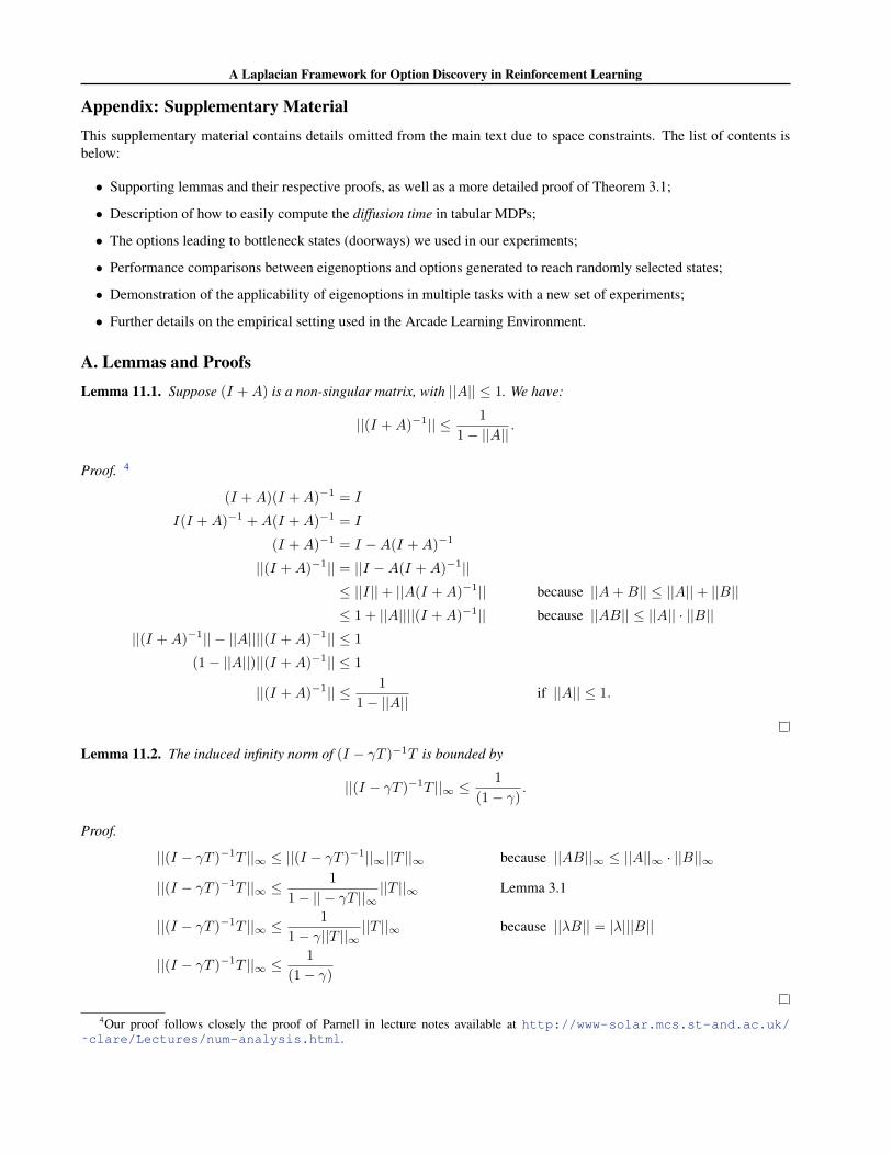
A. Lemmas and ProofsLemma 11.1. Suppose (I +A) is a non-singular matrix, with ||A|| ≤ 1. We have:

||(I +A)−1|| ≤ 1

1− ||A||.

Proof. 4

(I +A)(I +A)−1 = I

I(I +A)−1 +A(I +A)−1 = I

(I +A)−1 = I −A(I +A)−1

||(I +A)−1|| = ||I −A(I +A)−1||≤ ||I||+ ||A(I +A)−1|| because ||A+B|| ≤ ||A||+ ||B||≤ 1 + ||A||||(I +A)−1|| because ||AB|| ≤ ||A|| · ||B||

||(I +A)−1|| − ||A||||(I +A)−1|| ≤ 1

(1− ||A||)||(I +A)−1|| ≤ 1

||(I +A)−1|| ≤ 1

1− ||A||if ||A|| ≤ 1.

Lemma 11.2. The induced infinity norm of (I − γT )−1T is bounded by

||(I − γT )−1T ||∞ ≤1

(1− γ).

Proof.

||(I − γT )−1T ||∞ ≤ ||(I − γT )−1||∞||T ||∞ because ||AB||∞ ≤ ||A||∞ · ||B||∞

||(I − γT )−1T ||∞ ≤1

1− || − γT ||∞||T ||∞ Lemma 3.1

||(I − γT )−1T ||∞ ≤1

1− γ||T ||∞||T ||∞ because ||λB|| = |λ|||B||

||(I − γT )−1T ||∞ ≤1

(1− γ)

4Our proof follows closely the proof of Parnell in lecture notes available at http://www-solar.mcs.st-and.ac.uk/˜clare/Lectures/num-analysis.html.

http://www-solar.mcs.st-and.ac.uk/~clare/Lectures/num-analysis.html

http://www-solar.mcs.st-and.ac.uk/~clare/Lectures/num-analysis.html


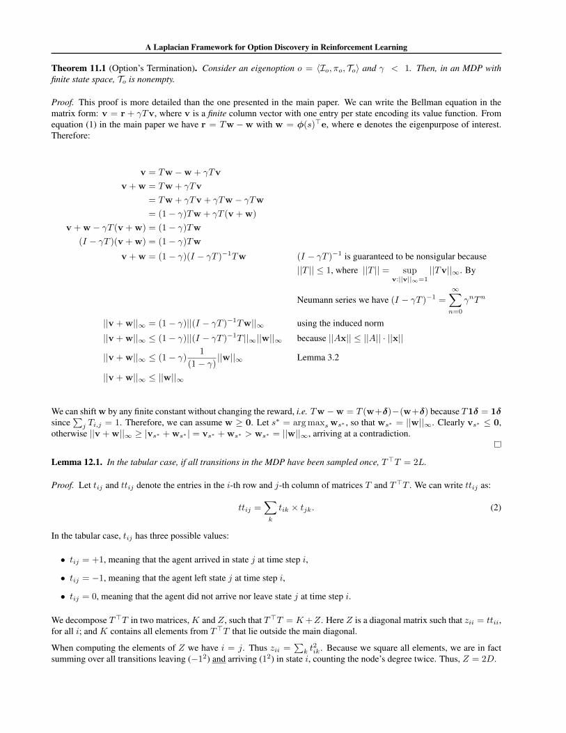
Theorem 11.1 (Option’s Termination). Consider an eigenoption o = 〈Io, πo, To〉 and γ < 1. Then, in an MDP withfinite state space, To is nonempty.

Proof. This proof is more detailed than the one presented in the main paper. We can write the Bellman equation in thematrix form: v = r + γTv, where v is a finite column vector with one entry per state encoding its value function. Fromequation (1) in the main paper we have r = Tw −w with w = φ(s)>e, where e denotes the eigenpurpose of interest.Therefore:

v = Tw −w + γTv

v + w = Tw + γTv

= Tw + γTv + γTw − γTw= (1− γ)Tw + γT (v + w)

v + w − γT (v + w) = (1− γ)Tw

(I − γT )(v + w) = (1− γ)Tw

v + w = (1− γ)(I − γT )−1Tw (I − γT )−1 is guaranteed to be nonsigular because||T || ≤ 1, where ||T || = sup

v:||v||∞=1

||Tv||∞. By

Neumann series we have (I − γT )−1 =

∞∑n=0

γnTn

||v + w||∞ = (1− γ)||(I − γT )−1Tw||∞ using the induced norm

||v + w||∞ ≤ (1− γ)||(I − γT )−1T ||∞||w||∞ because ||Ax|| ≤ ||A|| · ||x||

||v + w||∞ ≤ (1− γ)1

(1− γ)||w||∞ Lemma 3.2

||v + w||∞ ≤ ||w||∞

We can shift w by any finite constant without changing the reward, i.e. Tw −w = T (w+δ)−(w+δ) because T1δ = 1δsince

∑j Ti,j = 1. Therefore, we can assume w ≥ 0. Let s∗ = arg maxsws∗ , so that ws∗ = ||w||∞. Clearly vs∗ ≤ 0,

otherwise ||v + w||∞ ≥ |vs∗ + ws∗ | = vs∗ + ws∗ > ws∗ = ||w||∞, arriving at a contradiction.

Lemma 12.1. In the tabular case, if all transitions in the MDP have been sampled once, T>T = 2L.

Proof. Let tij and ttij denote the entries in the i-th row and j-th column of matrices T and T>T . We can write ttij as:

ttij =∑k

tik × tjk. (2)

In the tabular case, tij has three possible values:

• tij = +1, meaning that the agent arrived in state j at time step i,

• tij = −1, meaning that the agent left state j at time step i,

• tij = 0, meaning that the agent did not arrive nor leave state j at time step i.

We decompose T>T in two matrices, K and Z, such that T>T = K+Z. Here Z is a diagonal matrix such that zii = ttii,for all i; and K contains all elements from T>T that lie outside the main diagonal.

When computing the elements of Z we have i = j. Thus zii =∑k t

2ik. Because we square all elements, we are in fact

summing over all transitions leaving (−12) and arriving (12) in state i, counting the node’s degree twice. Thus, Z = 2D.


When not computing the elements in the main diagonal, for the element ttij , we add all transitions that leave state i arrivingin state j (−1 × 1), and those that leave state j arriving in state i (1 × −1). We assume each transition has been sampledonce, thus:

ttij =

{−2, if the transition between states i and j exists,

0, otherwise.

Therefore, we have K = −2W and T>T = K + Z = 2(D −W ).

B. Diffusion Time ComputationIn the main paper we introduced diffusion time as a new metric to evaluate exploration, but we did not discuss how it canbe computed. Diffusion time encodes the expected number of time steps required to navigate between any two states inthe MDP when following a random walk. In tabular domains, we can easily compute the diffusion time with dynamicprogramming. To do so we define a new MDP such that the value function of a state s, under a uniform random policy,encodes the expected number of steps required to navigate between state s and a chosen goal state. We can then computethe expected number of steps between any two states by averaging, for each possible goal, the value of all other states.

The MDP in which the value function of state s encodes the expected number of time steps from s to a goal state has γ = 1and a reward function where the agent observes +1 at every time step in which it is not in the goal state. Policy evaluationin this case encodes the expected number of time steps the agent will take before arriving to the goal state. To compute thediffusion time we iterate over all possible states, defining them as terminal states, and averaging the value function of theother states in that MDP.

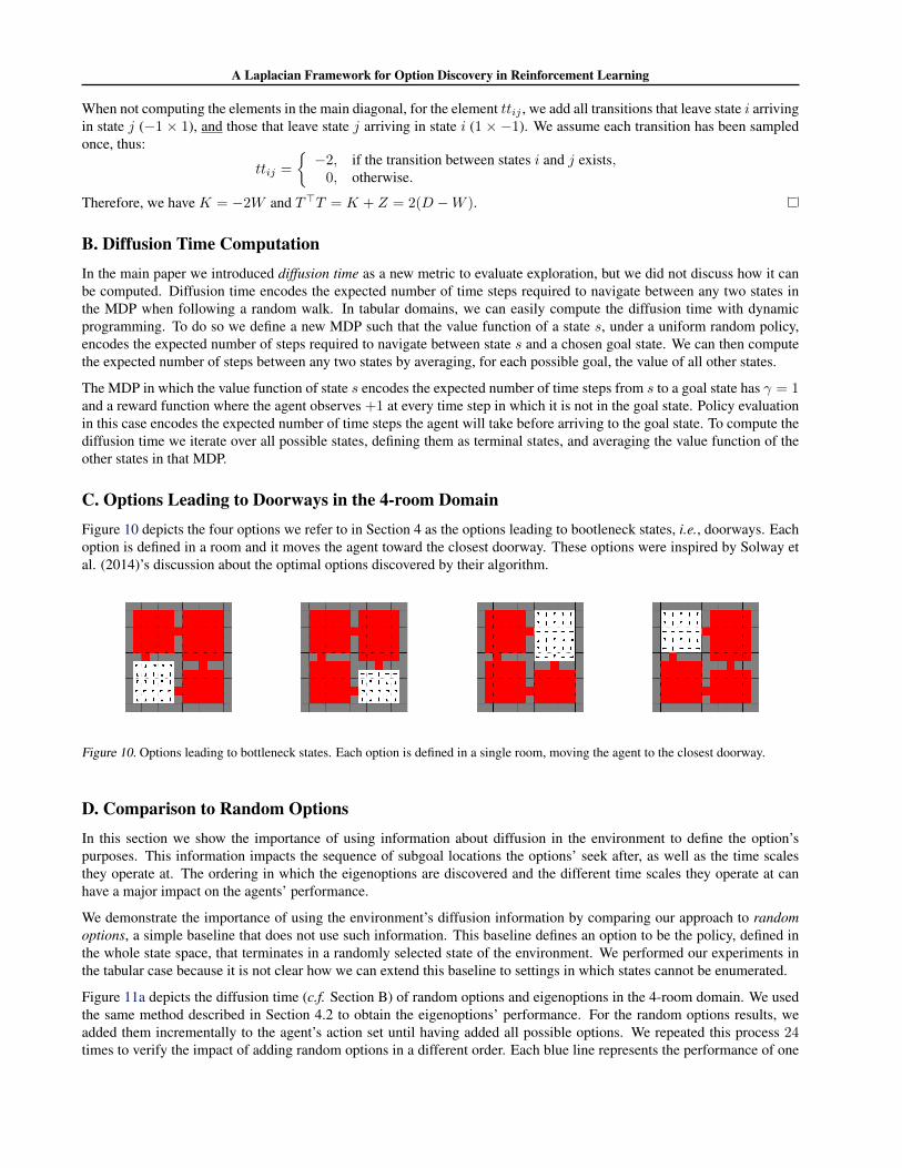
C. Options Leading to Doorways in the 4-room DomainFigure 10 depicts the four options we refer to in Section 4 as the options leading to bootleneck states, i.e., doorways. Eachoption is defined in a room and it moves the agent toward the closest doorway. These options were inspired by Solway etal. (2014)’s discussion about the optimal options discovered by their algorithm.

Figure 10. Options leading to bottleneck states. Each option is defined in a single room, moving the agent to the closest doorway.

D. Comparison to Random OptionsIn this section we show the importance of using information about diffusion in the environment to define the option’spurposes. This information impacts the sequence of subgoal locations the options’ seek after, as well as the time scalesthey operate at. The ordering in which the eigenoptions are discovered and the different time scales they operate at canhave a major impact on the agents’ performance.

We demonstrate the importance of using the environment’s diffusion information by comparing our approach to randomoptions, a simple baseline that does not use such information. This baseline defines an option to be the policy, defined inthe whole state space, that terminates in a randomly selected state of the environment. We performed our experiments inthe tabular case because it is not clear how we can extend this baseline to settings in which states cannot be enumerated.

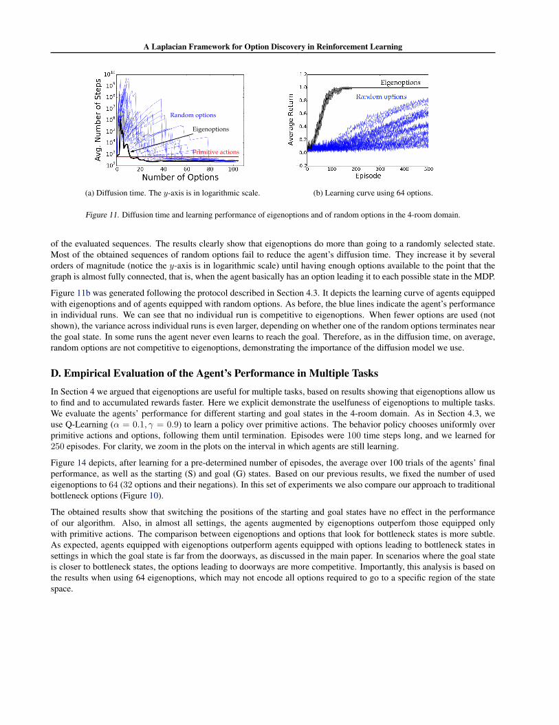
Figure 11a depicts the diffusion time (c.f. Section B) of random options and eigenoptions in the 4-room domain. We usedthe same method described in Section 4.2 to obtain the eigenoptions’ performance. For the random options results, weadded them incrementally to the agent’s action set until having added all possible options. We repeated this process 24times to verify the impact of adding random options in a different order. Each blue line represents the performance of one


Primitive actions

Eigenoptions

Random options

(a) Diffusion time. The y-axis is in logarithmic scale. (b) Learning curve using 64 options.

Figure 11. Diffusion time and learning performance of eigenoptions and of random options in the 4-room domain.

of the evaluated sequences. The results clearly show that eigenoptions do more than going to a randomly selected state.Most of the obtained sequences of random options fail to reduce the agent’s diffusion time. They increase it by severalorders of magnitude (notice the y-axis is in logarithmic scale) until having enough options available to the point that thegraph is almost fully connected, that is, when the agent basically has an option leading it to each possible state in the MDP.

Figure 11b was generated following the protocol described in Section 4.3. It depicts the learning curve of agents equippedwith eigenoptions and of agents equipped with random options. As before, the blue lines indicate the agent’s performancein individual runs. We can see that no individual run is competitive to eigenoptions. When fewer options are used (notshown), the variance across individual runs is even larger, depending on whether one of the random options terminates nearthe goal state. In some runs the agent never even learns to reach the goal. Therefore, as in the diffusion time, on average,random options are not competitive to eigenoptions, demonstrating the importance of the diffusion model we use.

D. Empirical Evaluation of the Agent’s Performance in Multiple TasksIn Section 4 we argued that eigenoptions are useful for multiple tasks, based on results showing that eigenoptions allow usto find and to accumulated rewards faster. Here we explicit demonstrate the uselfuness of eigenoptions to multiple tasks.We evaluate the agents’ performance for different starting and goal states in the 4-room domain. As in Section 4.3, weuse Q-Learning (α = 0.1, γ = 0.9) to learn a policy over primitive actions. The behavior policy chooses uniformly overprimitive actions and options, following them until termination. Episodes were 100 time steps long, and we learned for250 episodes. For clarity, we zoom in the plots on the interval in which agents are still learning.

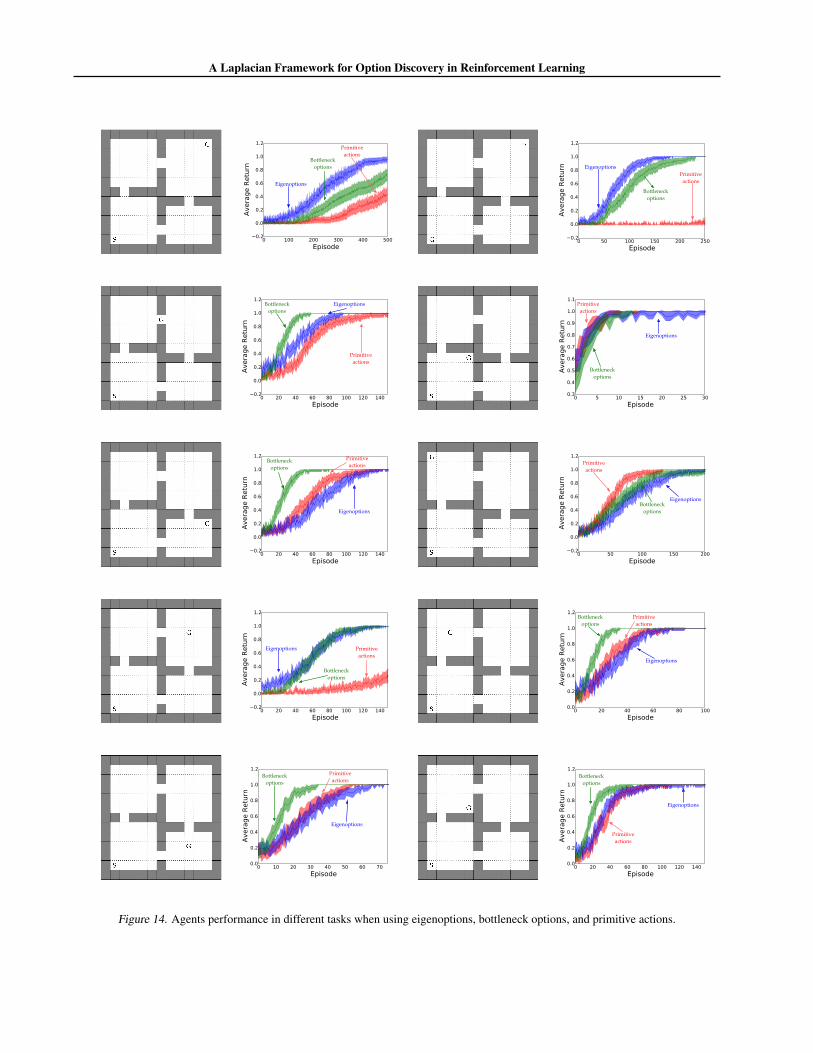
Figure 14 depicts, after learning for a pre-determined number of episodes, the average over 100 trials of the agents’ finalperformance, as well as the starting (S) and goal (G) states. Based on our previous results, we fixed the number of usedeigenoptions to 64 (32 options and their negations). In this set of experiments we also compare our approach to traditionalbottleneck options (Figure 10).

The obtained results show that switching the positions of the starting and goal states have no effect in the performanceof our algorithm. Also, in almost all settings, the agents augmented by eigenoptions outperfom those equipped onlywith primitive actions. The comparison between eigenoptions and options that look for bottleneck states is more subtle.As expected, agents equipped with eigenoptions outperform agents equipped with options leading to bottleneck states insettings in which the goal state is far from the doorways, as discussed in the main paper. In scenarios where the goal stateis closer to bottleneck states, the options leading to doorways are more competitive. Importantly, this analysis is based onthe results when using 64 eigenoptions, which may not encode all options required to go to a specific region of the statespace.


(a) FREEWAY (b) MONTEZUMA’S REVENGE (c) MS PAC-MAN

Figure 12. Pre-defined start states in Atari 2600 games.

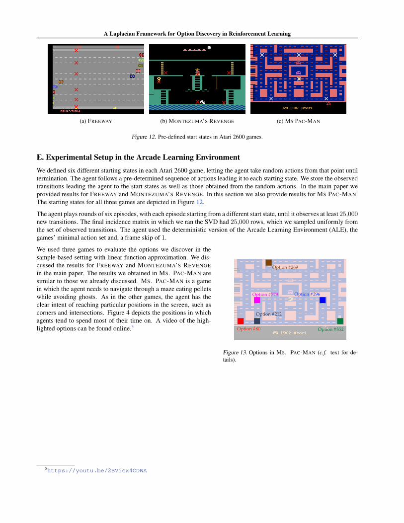
E. Experimental Setup in the Arcade Learning EnvironmentWe defined six different starting states in each Atari 2600 game, letting the agent take random actions from that point untiltermination. The agent follows a pre-determined sequence of actions leading it to each starting state. We store the observedtransitions leading the agent to the start states as well as those obtained from the random actions. In the main paper weprovided results for FREEWAY and MONTEZUMA’S REVENGE. In this section we also provide results for MS PAC-MAN.The starting states for all three games are depicted in Figure 12.

The agent plays rounds of six episodes, with each episode starting from a different start state, until it observes at least 25,000new transitions. The final incidence matrix in which we ran the SVD had 25,000 rows, which we sampled uniformly fromthe set of observed transitions. The agent used the deterministic version of the Arcade Learning Environment (ALE), thegames’ minimal action set and, a frame skip of 1.

Option #80

Option #212

Option #269

Option #852


Figure 13. Options in MS. PAC-MAN (c.f. text for de-tails).

We used three games to evaluate the options we discover in thesample-based setting with linear function approximation. We dis-cussed the results for FREEWAY and MONTEZUMA’S REVENGEin the main paper. The results we obtained in MS. PAC-MAN aresimilar to those we already discussed. MS. PAC-MAN is a gamein which the agent needs to navigate through a maze eating pelletswhile avoiding ghosts. As in the other games, the agent has theclear intent of reaching particular positions in the screen, such ascorners and intersections. Figure 4 depicts the positions in whichagents tend to spend most of their time on. A video of the high-lighted options can be found online.5

5https://youtu.be/2BVicx4CDWA

https://youtu.be/2BVicx4CDWA


Eigenoptions

Bottleneckoptions

Primitiveactions

Eigenoptions

Bottleneckoptions

Primitiveactions

EigenoptionsBottleneckoptions

Primitiveactions

Eigenoptions

Bottleneckoptions

Primitiveactions

Eigenoptions

Bottleneckoptions

Primitiveactions

EigenoptionsBottleneckoptions

Primitiveactions

Eigenoptions

Bottleneckoptions

Primitiveactions

Eigenoptions

Bottleneckoptions

Primitiveactions

Eigenoptions

Bottleneckoptions

Primitiveactions

Eigenoptions

Bottleneckoptions

Primitiveactions

Figure 14. Agents performance in different tasks when using eigenoptions, bottleneck options, and primitive actions.

a laplacian framework for option discovery in ... · a laplacian framework for option discovery in...

Documents