AIR QUALITY MODELING

AIR QUALITY MODELING (AQM) Predict pollutant concentrations at various locations

around the source.

Identify source contribution to air quality problems.

Assess source impacts and design control strategies.

Predict future pollutant concentrations from sources after implementation of new regulatory programs.

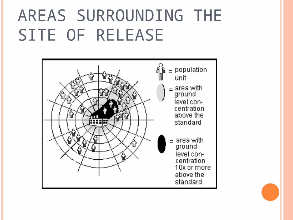
AREAS SURROUNDING THE SITE OF RELEASE

AIR QUALITY MODELING (AQM) Mathematical and numerical techniques are used in AQM to

simulate the dispersion of air pollutants.

Modeling of the dispersion of pollutants Toxic and odorous substances Single or multiple points Point, Area, or Volume sources

Input data required for Air Quality Modeling Source characteristics Meteorological conditions Site and surrounding conditions

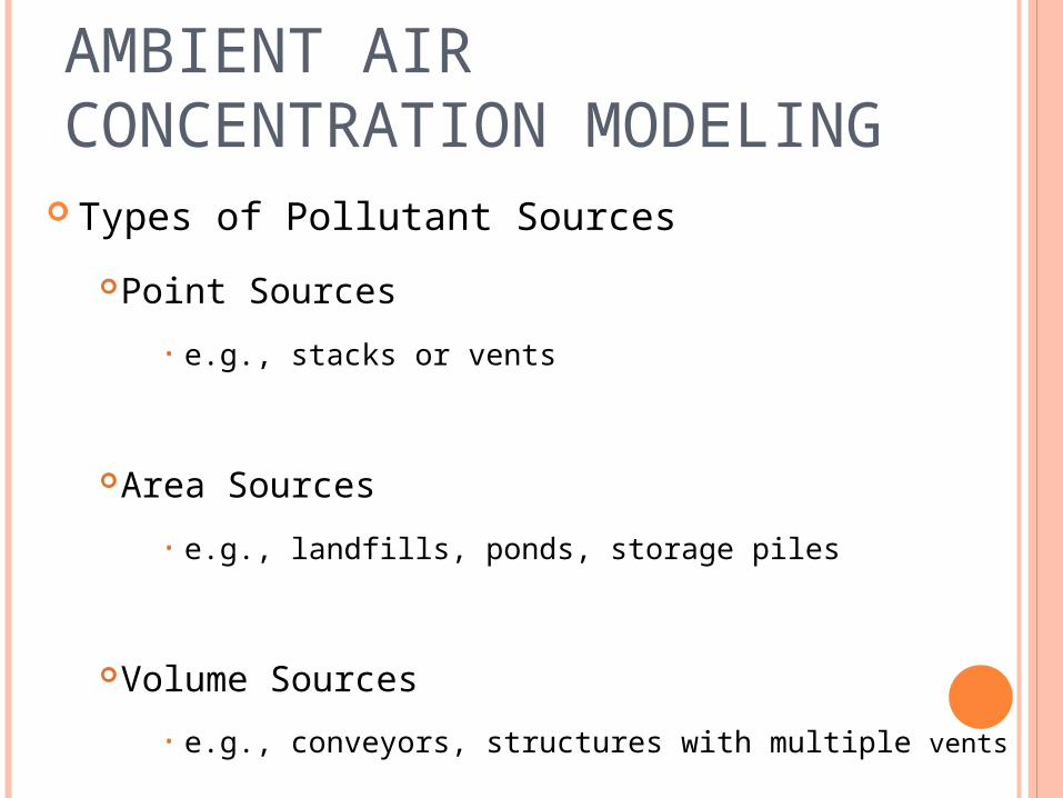
AMBIENT AIR CONCENTRATION MODELING

Types of Pollutant Sources

Point Sources

• e.g., stacks or vents

Area Sources

• e.g., landfills, ponds, storage piles

Volume Sources

• e.g., conveyors, structures with multiple vents

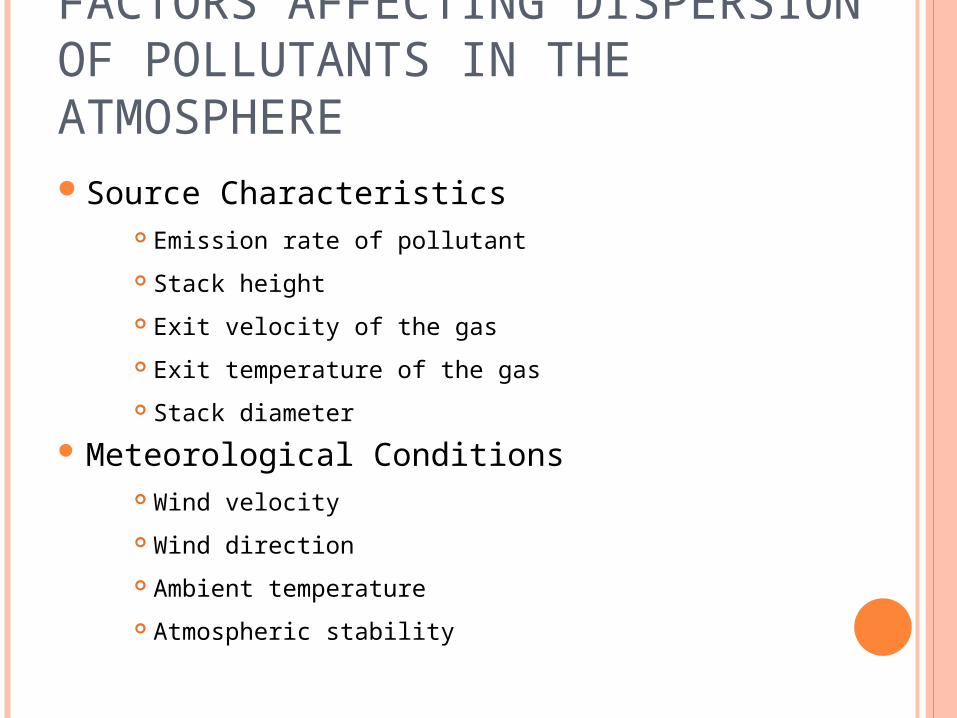
FACTORS AFFECTING DISPERSION OF POLLUTANTS IN THE ATMOSPHERESource Characteristics

Emission rate of pollutant

Stack height

Exit velocity of the gas

Exit temperature of the gas

Stack diameter

Meteorological Conditions Wind velocity

Wind direction

Ambient temperature

Atmospheric stability

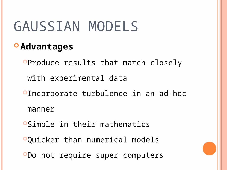
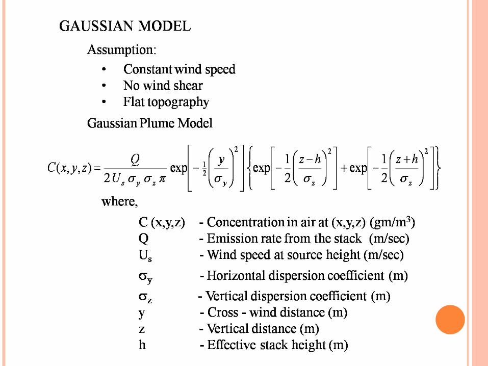
GAUSSIAN MODELS Advantages

Produce results that match closely with experimental

data

Incorporate turbulence in an ad-hoc manner

Simple in their mathematics

Quicker than numerical models

Do not require super computers

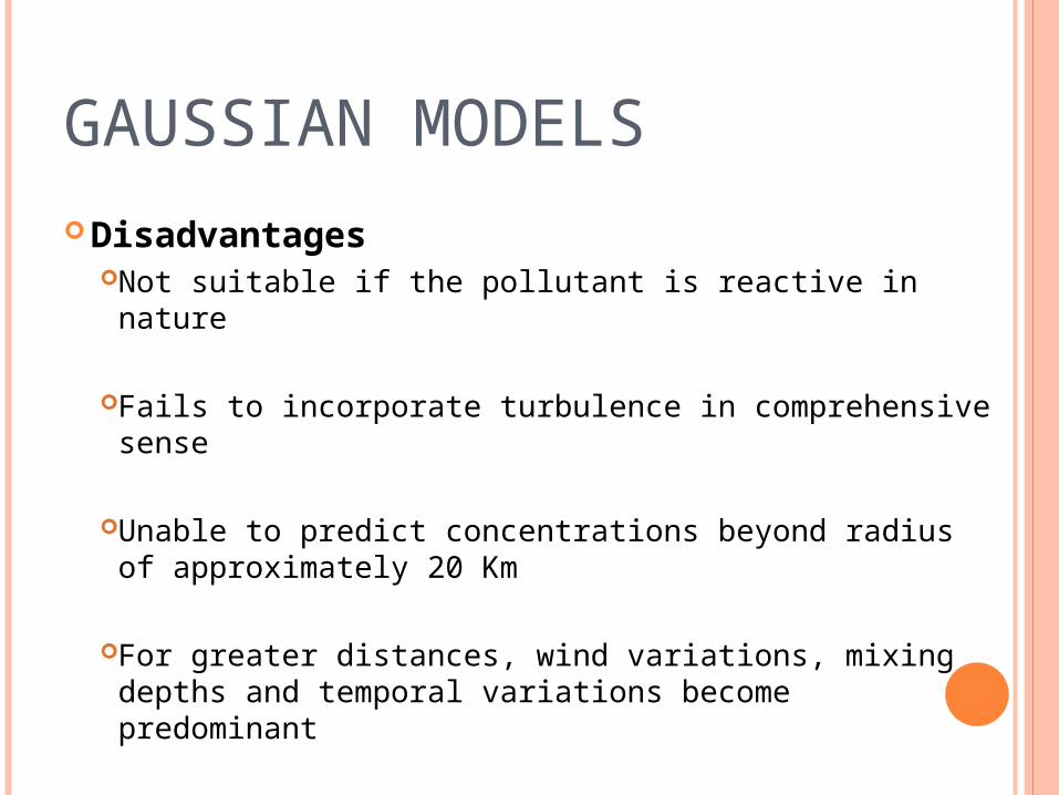
GAUSSIAN MODELS

DisadvantagesNot suitable if the pollutant is reactive in nature

Fails to incorporate turbulence in comprehensive sense

Unable to predict concentrations beyond radius of approximately 20 Km

For greater distances, wind variations, mixing depths and temporal variations become predominant

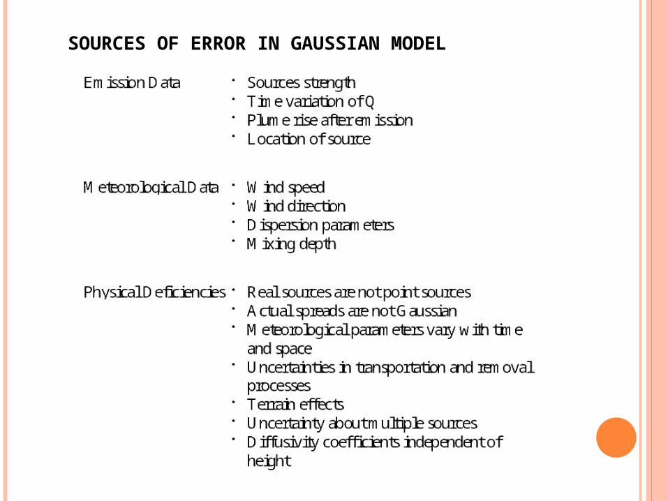
SOURCES OF ERROR IN GAUSSIAN MODEL

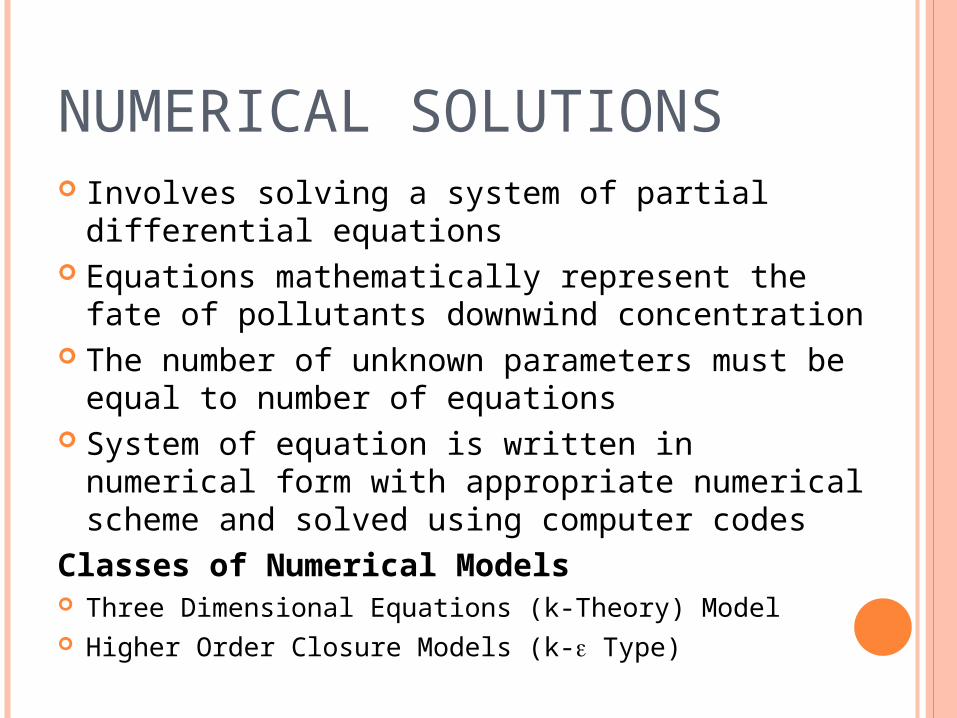
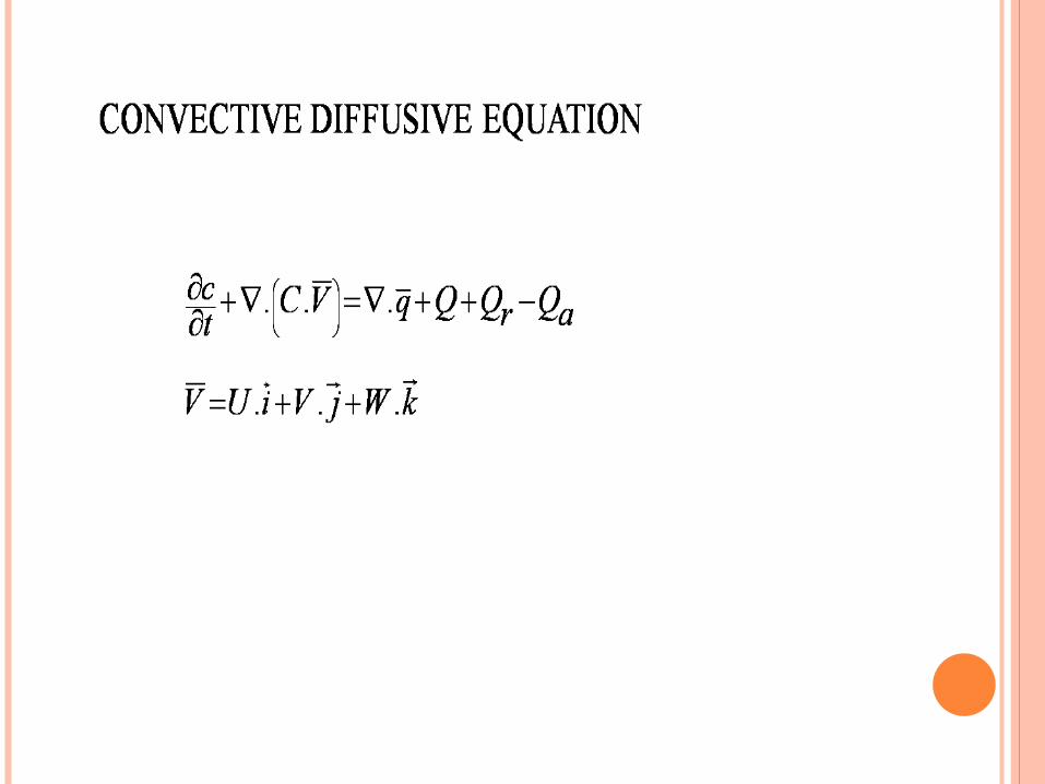
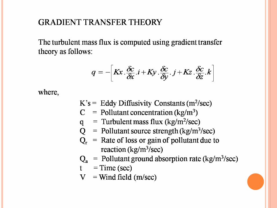
NUMERICAL SOLUTIONS Involves solving a system of partial differential equations Equations mathematically represent the fate of pollutants

downwind concentration The number of unknown parameters must be equal to

number of equations System of equation is written in numerical form with

appropriate numerical scheme and solved using computer codes

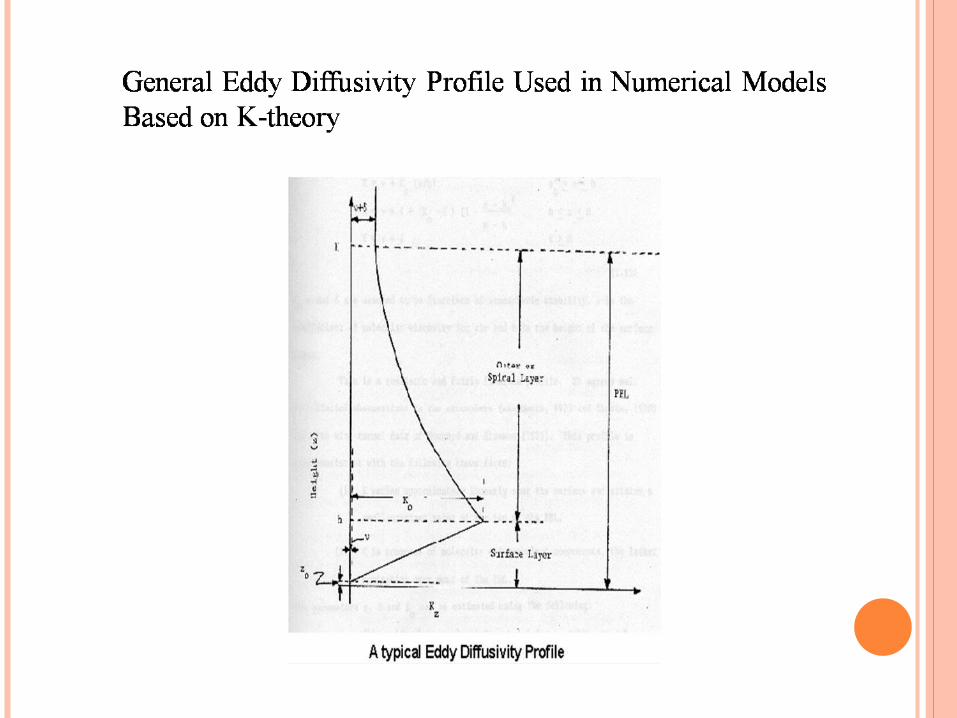
Classes of Numerical Models Three Dimensional Equations (k-Theory) Model Higher Order Closure Models (k- Type)

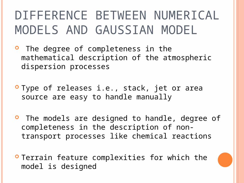
DIFFERENCE BETWEEN NUMERICAL MODELS AND GAUSSIAN MODEL The degree of completeness in the mathematical

description of the atmospheric dispersion processes

Type of releases i.e., stack, jet or area source are easy to handle manually

The models are designed to handle, degree of completeness in the description of non-transport processes like chemical reactions

Terrain feature complexities for which the model is designed

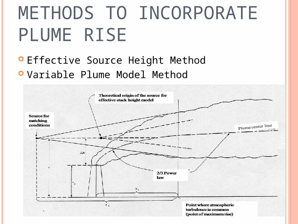
METHODS TO INCORPORATE PLUME RISE Effective Source Height Method Variable Plume Model Method

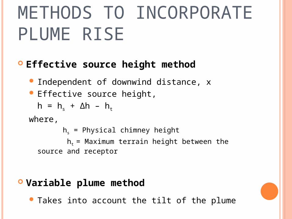
METHODS TO INCORPORATE PLUME RISE Effective source height method

Independent of downwind distance, x Effective source height,

h = hs + ∆h – ht

where, hs = Physical chimney height

ht = Maximum terrain height between the source and receptor

Variable plume method

Takes into account the tilt of the plume

PROBLEM

Calculate the nighttime concentration of nitrogen oxides 1 km downward of an open, burning dump if the dump emits NOx at the rate of 4 g/sec. The wind speed is 4 m/sec at 10 m above ground level. The one-hour average diffusion coefficients at 1 km are estimated as sy = 70 m and sz = 50 m and the dump is assumed to be a point source.

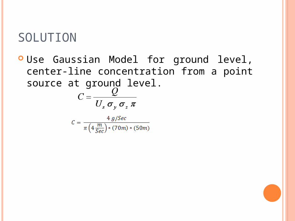
SOLUTION

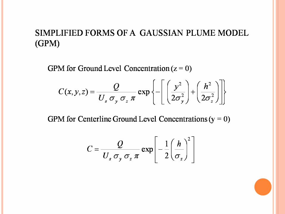
Use Gaussian Model for ground level, center-line concentration from a point source at ground level.

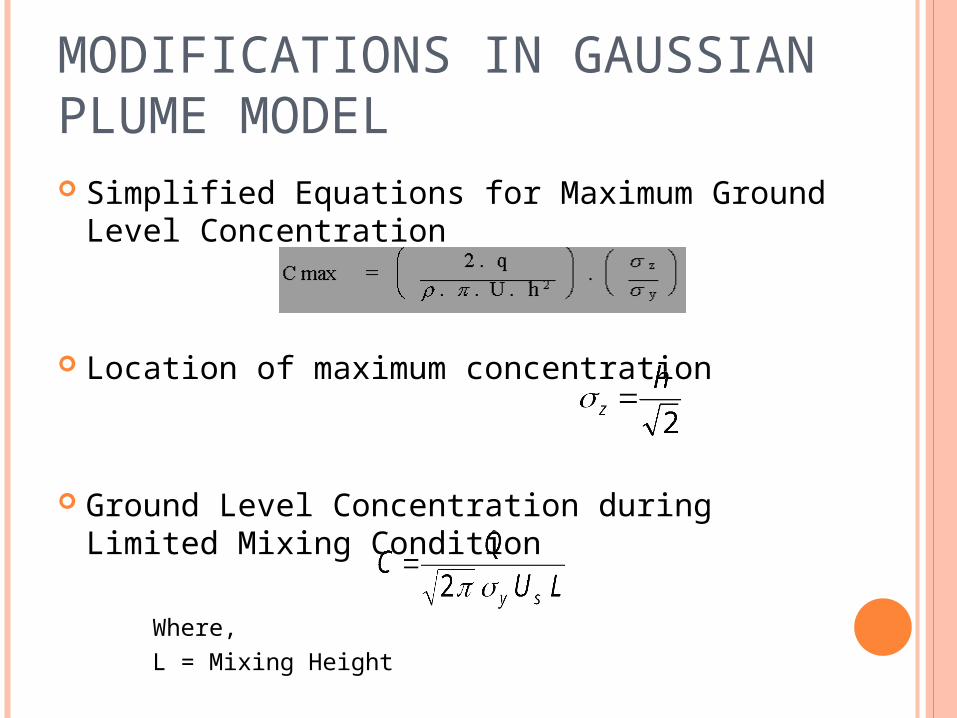
MODIFICATIONS IN GAUSSIAN PLUME MODEL Simplified Equations for Maximum Ground Level

Concentration

Location of maximum concentration

Ground Level Concentration during Limited Mixing Condition

Where,L = Mixing

Height

Concentration Estimate for Various Sampling Times

C2 = C1 (t1/t2) q

where,q lies between 0.17 and 0.5

Average Time Multiplying Factor

3 hours 0.9 (±0.1)

8 hours 0.7 (±0.1)

24 hours 0.4 (±0.1)

PLUME DISPERSION PARAMETERS

Different Methods to Calculate SigmasExperimental data

Modified Experimental Curves

Lagrangian Auto Correlation Function

Moment-Concentration Method

Taylor's Statistical Theory

PLUME DISPERSION PARAMETERS

Factors Considered while Calculating SigmasNature of Release

Sampling Time

Release Height

Terrain Features

Velocity Field

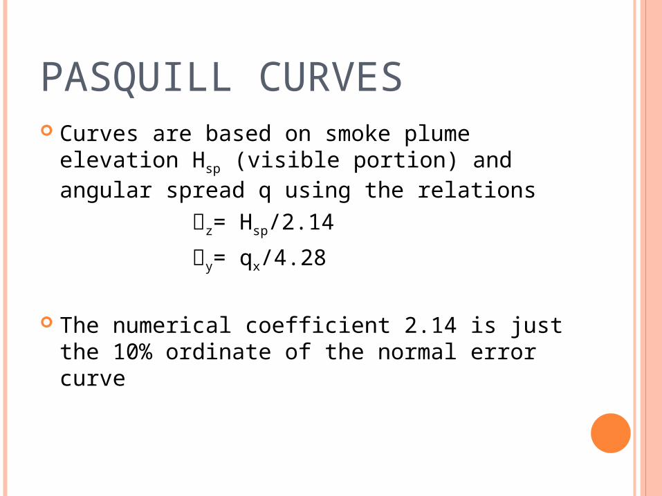
PASQUILL CURVES Curves are based on smoke plume elevation Hsp (visible

portion) and angular spread q using the relationsz= Hsp/2.14

y= qx/4.28

The numerical coefficient 2.14 is just the 10% ordinate of the normal error curve

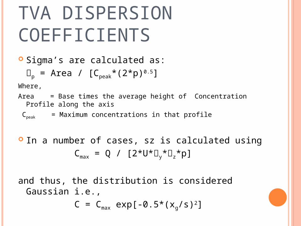
TVA DISPERSION COEFFICIENTS Sigma’s are calculated as:

p = Area / [Cpeak*(2*p)0.5]Where,

Area = Base times the average height of Concentration Profile along the axis

Cpeak = Maximum concentrations in that profile

In a number of cases, sz is calculated using Cmax = Q / [2*U*y*z*p]

and thus, the distribution is considered Gaussian i.e., C = Cmax exp[-0.5*(xg/s)2]

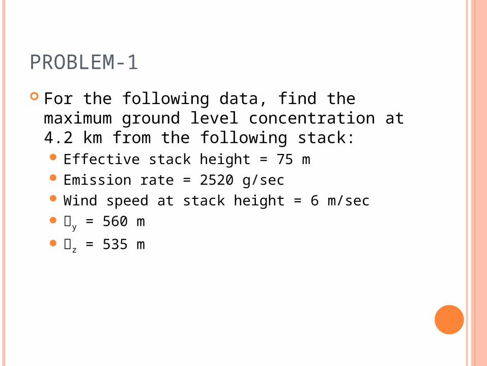
PROBLEM-1

For the following data, find the maximum ground level concentration at 4.2 km from the following stack: Effective stack height = 75 m Emission rate = 2520 g/sec Wind speed at stack height = 6 m/sec y = 560 m z = 535 m

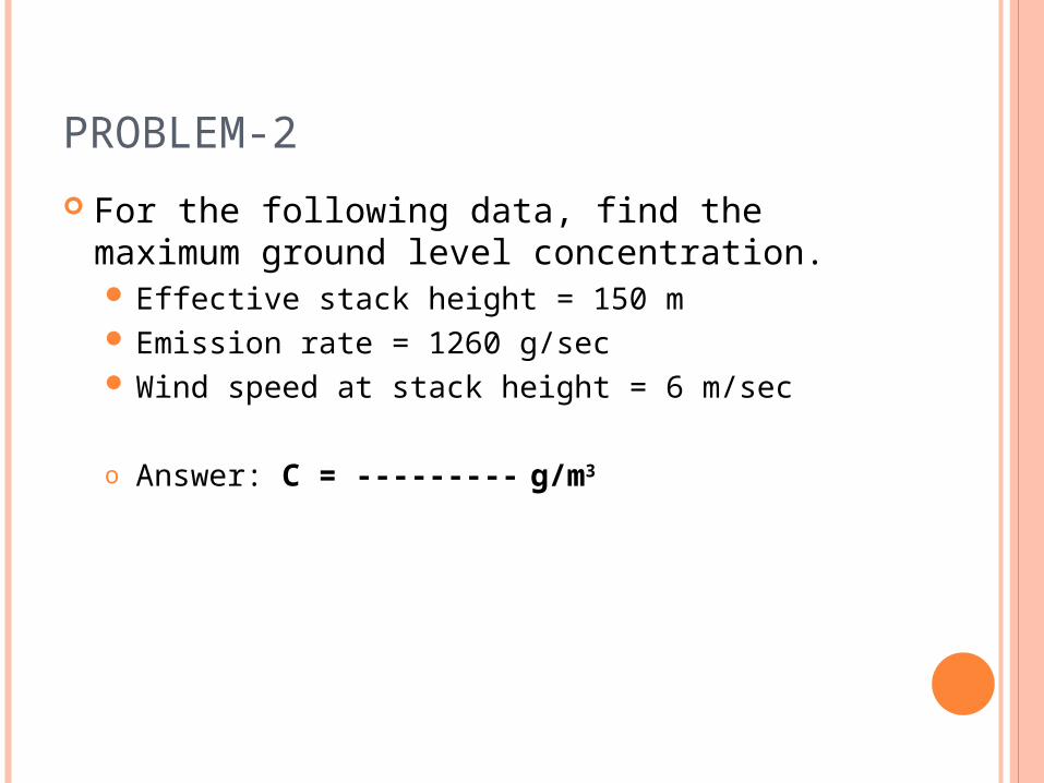
PROBLEM-2

For the following data, find the maximum ground level concentration. Effective stack height = 150 m Emission rate = 1260 g/sec Wind speed at stack height = 6 m/sec

o Answer: C = --------- g/m3