A hyperbolic model for convection-diffusion

transport problems in CFD: Numerical

analysis and applications

Hector Gomez, Ignasi Colominas ∗, Fermın Navarrina andManuel Casteleiro

Group of Numerical Methods in Engineering, GMNIDept. of Applied Mathematics, School of Civil Engineering

Universidad de A CorunaCampus de Elvina, 15071 A Coruna, Spain

Abstract

In this paper we present a numerical study of a hyperbolic model for convection-diffusion transport problems that has been recently proposed by the authors [1].This model avoids the infinite speed paradox, inherent to the standard parabolicmodel and introduces a new parameter τ called relaxation time. This parameterplays the role of an “inertia” for the movement of the pollutant.

The analysis presented herein is twofold: firstly, we perform an accurate study ofthe 1D steady equations and its numerical solution. We compare the solution of thehyperbolic model with that of the parabolic model and we analyze the influence ofthe relaxation time on the solution. On the other hand, we explore the possibilitiesof the proposed model for real computations in engineering. With this aim we solvean example concerning the evolution of a pollutant being spilled in the harbor of ACoruna (northwest of SPAIN, EU).

Key words: Convection-Diffusion, Cattaneo’s equation, Finite velocity.

∗ Correspondence to: E.T.S. de Ingenieros de Caminos, Canales y Puertos, Univer-sidad de A Coruna, Campus de Elvina, 15071 A Coruna, Spain.

Email address: icolominas@udc.es (Ignasi Colominas).

Preprint submitted to Elsevier Science 23 October 2006

1 Introduction

There is much experimental evidence which proves that diffusive processestake place with finite velocity inside matter [2,3]. However, standard parabolicmodels based on Fick’s law [4] or Fourier’s law [5] (in the case of mass transportor heat conduction respectively) predict an infinite speed of propagation. Insome applications, this issue can be ignored and the use of parabolic modelsis assumed to be accurate enough for practical purposes in spite of predictingan infinite speed of propagation [6]. However, in many other applications itis necessary to take into account the wave nature of diffusive processes toperform accurate predictions [2,7]. This kind of approach cannot be carriedout by using Fick’s law or Fourier’s law. Instead a more general constitutivelaw, for example the one proposed by Cattaneo [6], must be employed.

In the past, the study of the hyperbolic diffusion has been limited to pure-diffusive problems [8–11]. Recently the authors have proposed a generalizationof the hyperbolic diffusion equation that can also be used in convective cases[12–14]. From a numerical point of view, the simulation of the hyperbolic diffu-sion equation has been mostly limited to 1D problems [15,16]. The numericaldiscretization of 2D pure-diffusion problems was probably pioneered by Yang[17]. Later, Manzari et al. [18] proposed a different algorithm and solved somepractical pure-diffusive examples.

The first objective of this paper is to perform an accurate analysis of the1D steady convection-diffusion equation and its numerical solution. We com-pare the parabolic and the hyperbolic models by means of their numericaland exact solutions. The objective is to analyze whether the infinite speedparadox (inherent to the parabolic model) contributes or not to the numericalinstabilities that appear in convection dominated flows discretized with cen-tered methods. The fact is that there is a well-known example that may berelated to the one presented herein. In the context of CFD, the assumptionof incompressibility leads to the result that pressure waves can travel at aninfinite speed. The velocity of pressure waves becomes finite when one removesthis assumption and many of the problems that appear in the numerical res-olution of incompressible flow problems do not appear in compressible fluidcomputations.

The second objective of this paper is to explore the possibilities of the hyper-bolic model for practical computations in engineering in the context of massdiffusion within a fluid. In this framework, there are a lot of important appli-cations in civil and environmental engineering, for instance, the prediction ofthe fate of a pollutant spilled in a fluid. This paper presents an example con-cerning the evolution of a pollutant being spilled in the harbor of A Coruna(northwest of SPAIN, EU).

2

The outline of this paper is as follows: In Section 2 we review the parabolicformulation of the convective-diffusive equation. In section 3 we present thehyperbolic model for the transport problem. A numerical analysis of the 1Dsteady state equations is performed in section 4. In section 5 we solve a prac-tical case in environmental engineering. Finally, section 6 is devoted to thepresentation of the main conclusions of this study.

2 Standard formulation of the convection-diffusion transport prob-lem

In this section we review the classic formulation for the convection-diffusiontransport problem. We assume the medium to be incompressible and we donot consider source terms. The governing equations under these hypothesesare as follows:

∂u

∂t+ a · ∇x (u) +∇x · (q) = 0 (1.1)

q = −K∇x (u) (1.2)

In the above system, (1.1) is the mass conservation equation and (1.2) is theconstitutive equation known as Fick’s law. Furthermore, u is the pollutantconcentration, a is the velocity field which satisfies the hydrodynamic equa-tions of an incompressible fluid, q is the diffusive flux per unit fluid density andK is the diffusivity tensor which is assumed to be positive definite. Clearly,system (1) can be decoupled since we can introduce (1.2) into (1.1) and solvethe scalar equation

∂u

∂t+ a · ∇x (u)−∇x · (K∇x (u)) = 0 (2)

It is well known that equation (2) is parabolic. Therefore, boundary conditionsmust be imposed everywhere on the boundary of the domain [20]. Then, let usconsider the transport by convection and diffusion in a domain Ω ⊂ R2 withpiecewise smooth boundary Γ. The unit outward normal vector to Γ is denotedby n. The boundary is assumed to consist of a portion ΓD on which the valueof u is prescribed (Dirichlet or essential conditions) and a complementaryportion ΓN on which flux is prescribed (Neumann or natural conditions). Inaddition, we know the initial distribution of the transported quantity u. Atthis point we can state convection-diffusion initial-boundary value problem asfollows: given a divergence free velocity field a, given the diffusion tensor Kand given adequate initial and boundary conditions, find u : Ω × [0, T ] 7→ R

3

such that

∂u

∂t+ a · ∇x (u)−∇x · (K∇x (u)) = 0 in Ω× [0, T ] (3.1)

u(x, 0) = u0(x) on Ω (3.2)

u = uD on ΓD × (0, T ] (3.3)

K∇x (u) · n = h on ΓN × (0, T ] (3.4)

3 A hyperbolic model for convection-diffusion problems

3.1 Governing equations

The hyperbolic model for convection-diffusion problems is obtained by substi-tuting Fick’s law (equation (1.2)) by a more general equation based on Cat-taneo’s law. Cattaneo’s equation was originally proposed for non-advectiveproblems and it can not be used directly for convection-diffusion problems.For this reason the authors have recently proposed [12–14] the following con-stitutive equation:

q + τ

(∂q

∂t+∇x (q) a

)= −K∇x (u) (4)

which can be used when the medium is moving with velocity a. Equation(4) has been derived from Cattaneo’s law by imposing Galilean invarianceprinciple to the resulting model. In this way, the description of the diffusionprocess is granted to be the same in every inertial frame [19].

Equation (4) can be closed by using the mass conservation equation. To derivethe mass conservation equation we will suppose the medium to be incompress-ible and we will not consider source terms. In this way, the governing equationsare as follows:

∂u

∂t+ a · ∇x (u) +∇x · (q) = 0 (5.1)

q + τ

(∂q

∂t+∇x (q) a

)= −K∇x (u) (5.2)

It should be noted that system (5) constitutes a generalization of the clas-sic parabolic convection-diffusion model since we can recover the standardformulation by setting τ = 0.

4

3.2 Conservative form

System (5) can be written as one single second order partial differential equa-tion when the velocity field is constant; otherwise, it must be solved as acoupled system of first order partial differential equations [12].

If we introduce the hypothesis that τ is a regular matrix (this appears tobe reasonable; in fact, it seems natural to demand τ to be positive-definitesince it is somehow representing a characteristic time of the diffusion process)and we use again that the fluid medium is incompressible, system (5) can bewritten as a system of conservation laws as follows:

∂u

∂t+∇x · (ua + q) = 0 (6.1)

∂q

∂t+∇x · (q ⊗ a + τ−1Ku) = u∇x · (τ−1K)− τ−1q (6.2)

For the sake of simplicity we will consider from here on the medium to behomogeneous and isotropic (hence, K = kI, τ = τI for certain k, τ ∈ R+).Under these hypotheses, system (6) can be written as

∂u

∂t+∇x · (ua + q) = 0 (7.1)

∂(τq)

∂t+∇x · (τq ⊗ a + kuI) + q = 0 (7.2)

In what follows one and two-dimensional problems will be studied separately.

3.2.1 One-dimensional problem

In this section we will study the one-dimensional Cattaneo-type transportproblem. In this simple case the governing equation is

∂U

∂t+∇x · (F ) = S (8)

where

U =

u

τq

; F =

ua + q

τqa + ku

; S =

0

−q

(9)

System (8) can be written in a non-conservative form as

∂U

∂t+ A

∂U

∂x= S (10)

5

being A the so-called Jacobian matrix defined by

A = ∇U (F ) =

a 1/τ

k a

(11)

It is well known (see for instance reference [20]) that system (8) will be totallyhyperbolic if, and only if, matrix A yields 2 different real eigenvalues. It canbe shown that

A = CDC−1 where C =

1 1

τc −τc

; D =

a + c 0

0 a− c

(12)

being

c =√

k/τ (13)

the celerity of the pollutant wave.

As a consequence, system (8) is totally hyperbolic. Now we will prove thatsystem (10) can be diagonalized but it can not be decoupled. The so-calledRiemann quasi-invariants can be defined (we call Riemann quasi-invariantsthose functions instead of Riemann invariants [20] because there is a sourceterm in (8)). To prove this fact, we use (12). Hence, we can rewrite (10) asfollows:

∂U

∂t+ CDC−1∂U

∂x= S (14)

As a consequence of the assumption of homogeneity, (14) takes the form

∂(C−1U )

∂t+ D

∂(C−1U )

∂x= C−1S (15)

If we use the notationR1

R2

= R = C−1U =1

2

u + q/c

u− q/c

(16)

for Riemann quasi-invariants the following equation holds:

∂R

∂t+ D

∂R

∂x= QR (17)

where Q is the matrix

Q =1

2τ

−1 1

1 −1

(18)

Therefore, since D is a diagonal matrix (and Q is not a diagonal one), system(17) is only coupled by the source term. The two scalar equations in (17) are

6

two transport equations with a source term. The quantity R1 is transportedalong the spatial coordinate with velocity a + c. Whereas, R2 is also trans-ported along the spatial coordinate in this case with velocity a − c. Hence,the direction in which each wave R1 or R2 is transported along the spatialcoordinate depends on the sign of its corresponding velocity of propagation.Therefore, depending on the values of a and c the solution of (17) can be thesuperposition of two waves traveling in the same or in the opposite direction.We will refer to this situation as supercritical and subcritical flow respectively.At this point it is useful to introduce the following dimensionless number:

H =|a|c

(19)

This number plays a similar role to Mach number in compressible flow prob-lems [21] or Froude number in shallow water problems [22]. By using thisdimensionless number we can differentiate three kinds of flow

• H < 1 ⇔ Subcritical flow• H > 1 ⇔ Supercritical flow• H = 1 ⇔ Critical flow

Taking into account all of this, boundary conditions which should be imposedto (17) are straightforward. Let us suppose that we have to solve (17) in agiven domain Ω = (0, L); L ∈ R+ which is bounded by Γ. We will call inflowboundary (Γin in what follows) the part of the boundary in which a · n < 0.We will call outflow boundary (Γout in short) the complementary part of theboundary. Now, we define Γ0 as the point x = 0 and ΓL as x = L. Accordingly,Γ = Γ0 ∪ΓL. In supercritical flow both R1 and R2 should be prescribed in theinflow boundary (Γ0 when a > 0 and ΓL when a < 0). If the flow is subcriticalthe quantity R1 should be prescribed in Γ0 and R2 must be imposed in ΓL .

However, it is commonly accepted [23] that a hyperbolic system of partialdifferential equations like (8) is well-posed when the number of imposed com-ponents of U on one boundary equals the number of negative eigenvaluesof the jacobian matrix. Therefore, in supercritical flow conditions both com-ponents of U should be prescribed on the inflow boundary and no compo-nents of U must be imposed on the outflow boundary. In subcritical flowone component of U should be prescribed on the inflow boundary and theother one must be imposed on the outflow boundary. In what follows, com-ponents of U prescribed on the boundary will be called inflow components ofU . These functions will be denoted as U in. Therefore, the one-dimensionalCattaneo-type transport problem can be stated as follows: given k, τ > 0,given the field velocity a and given adequate initial and boundary conditions,

7

find U : Ω× [0, T ] 7→ R2 such that

∂U

∂t+∇x · (F ) = S in Ω× [0, T ] (20.1)

U (x, 0) = U 0(x) on Ω (20.2)

U in = U inD on Γ× [0, T ] (20.3)

being U , F and S the vectors defined in (9).

3.2.2 Two-dimensional problem

The 2D counterpart of the study presented in section 3.2.1 can be found in[1,24]. We only present herein the conservative form of the equations:

∂U

∂t+∇x · (F ) = S (21)

where

U =

u

τq1

τq2

; F =

ua1 + q1 ua2 + q2

τq1a1 + ku τq1a2

τq2a1 τq2a2 + ku

; S =

0

−q1

−q2

(22)

Note that we have used the notation q = (q1, q2)T and a = (a1, a2)

T .

4 Numerical analysis of the 1D steady state Cattaneo-type convection-diffusion equations

4.1 The negative diffusion introduced by Cattaneo’s law

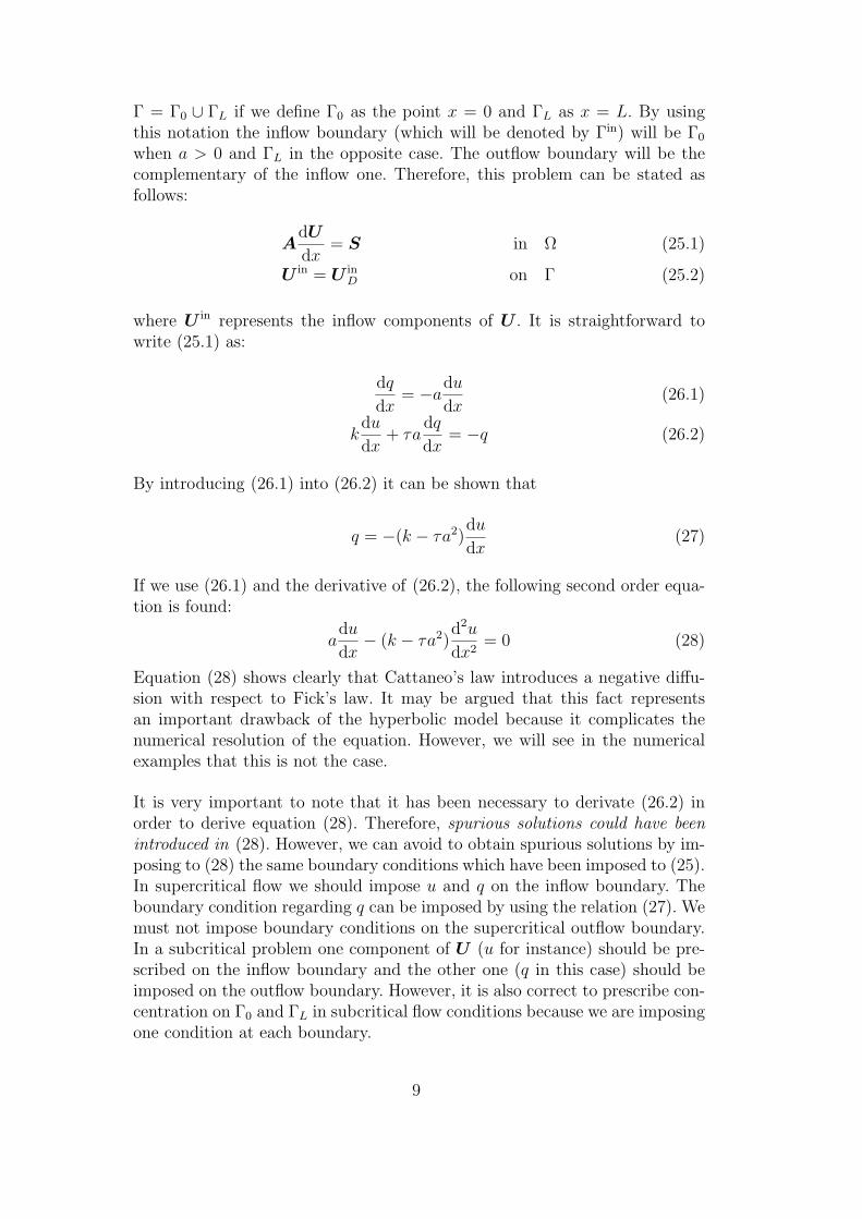
In this section we will show that Cattaneo’s law introduces a negative diffusionwith respect to Fick’s law. The governing equations in this case are:

∇x · (F ) = S (23)

being F and S the vectors defined in (9). The above equation can be writtenin non-conservative form as follows:

AdU

dx= S (24)

where U is the vector defined in (9) and A is the Jacobian matrix defined in(11). Let us consider the domain Ω = (0, L), L ∈ R+ bounded by Γ. Clearly,

8

Γ = Γ0 ∪ ΓL if we define Γ0 as the point x = 0 and ΓL as x = L. By usingthis notation the inflow boundary (which will be denoted by Γin) will be Γ0

when a > 0 and ΓL in the opposite case. The outflow boundary will be thecomplementary of the inflow one. Therefore, this problem can be stated asfollows:

AdU

dx= S in Ω (25.1)

U in = U inD on Γ (25.2)

where U in represents the inflow components of U . It is straightforward towrite (25.1) as:

dq

dx= −a

du

dx(26.1)

kdu

dx+ τa

dq

dx= −q (26.2)

By introducing (26.1) into (26.2) it can be shown that

q = −(k − τa2)du

dx(27)

If we use (26.1) and the derivative of (26.2), the following second order equa-tion is found:

adu

dx− (k − τa2)

d2u

dx2= 0 (28)

Equation (28) shows clearly that Cattaneo’s law introduces a negative diffu-sion with respect to Fick’s law. It may be argued that this fact representsan important drawback of the hyperbolic model because it complicates thenumerical resolution of the equation. However, we will see in the numericalexamples that this is not the case.

It is very important to note that it has been necessary to derivate (26.2) inorder to derive equation (28). Therefore, spurious solutions could have beenintroduced in (28). However, we can avoid to obtain spurious solutions by im-posing to (28) the same boundary conditions which have been imposed to (25).In supercritical flow we should impose u and q on the inflow boundary. Theboundary condition regarding q can be imposed by using the relation (27). Wemust not impose boundary conditions on the supercritical outflow boundary.In a subcritical problem one component of U (u for instance) should be pre-scribed on the inflow boundary and the other one (q in this case) should beimposed on the outflow boundary. However, it is also correct to prescribe con-centration on Γ0 and ΓL in subcritical flow conditions because we are imposingone condition at each boundary.

9

4.2 The effect of the standard Galerkin discretization on the classic parabolicconvection-diffusion equation

In this section we prove that (under the necessary assumptions) when a stan-dard Galerkin discretization is applied to the classic parabolic convection-diffusion equation, the velocity of propagation is not infinite anymore. On thecontrary, a finite velocity of propagation can be identified in the discrete equa-tions. By means of a comparison with the hyperbolic model we conclude thatthe standard Galerkin formulation introduces an “artificial” relaxation time.

We will carry on this study by analyzing the classic parabolic convection-diffusion problem subjected to homogeneous Dirichlet boundary conditions.Therefore, we state the following problem: find a function u : [0, L] 7→ R suchthat

adu

dx− k

d2u

dx2= 0; x ∈ (0, L) (29.1)

u(0) = u0 (29.2)

u(L) = uL (29.3)

Let 0 = x0 < x1 < · · · < xN = L be a uniform partition of the interval [0, L].We call h the distance between two consecutive nodes. Let us call

Pe =ah

2k(30)

the mesh Peclet number which expresses the ratio of convective to diffusivetransport. If we solve (29) by using the standard Galerkin method and linearfinite elements we obtain the following discrete equation at an interior node j[25]:

(1− Pe)uj+1 − 2uj + (1 + Pe)uj−1 = 0 (31)

In the above equation uj is the finite element approximation of u(xj) andu0, uN are the values given by the boundary conditions of (29). In addition,difference equations (31) can be solved exactly (see, for instance, reference[26]) since they are linear equations. The exact solution of (31) (subject toboundary conditions (29.2) and (29.3)) is

uj =1

1−(

1+Pe

1−Pe

)N

u0

[(1 + Pe

1− Pe

)j

−(

1 + Pe

1− Pe

)N]

+ uL

[1−

(1 + Pe

1− Pe

)j](32)

so oscillations will occur when |Pe| > 1.

On the other hand, the exact solution of (29) is

u(xj) =1

1− eahk

N

[u0

(e

ahk

j − eahk

N)

+ uL

(1− e

ahk

j)]

(33)

10

−1 −0.8 −0.6 −0.4 −0.2 0 0.2 0.4 0.6 0.8 10

0.2

0.4

0.6

0.8

1

Peclet number

Dimensionless diffusivity

−1 −0.8 −0.6 −0.4 −0.2 0 0.2 0.4 0.6 0.8 10

0.1

0.2

0.3

0.4

0.5

0.6

0.7

0.8

0.9

1

Peclet number

Dimensionless number H

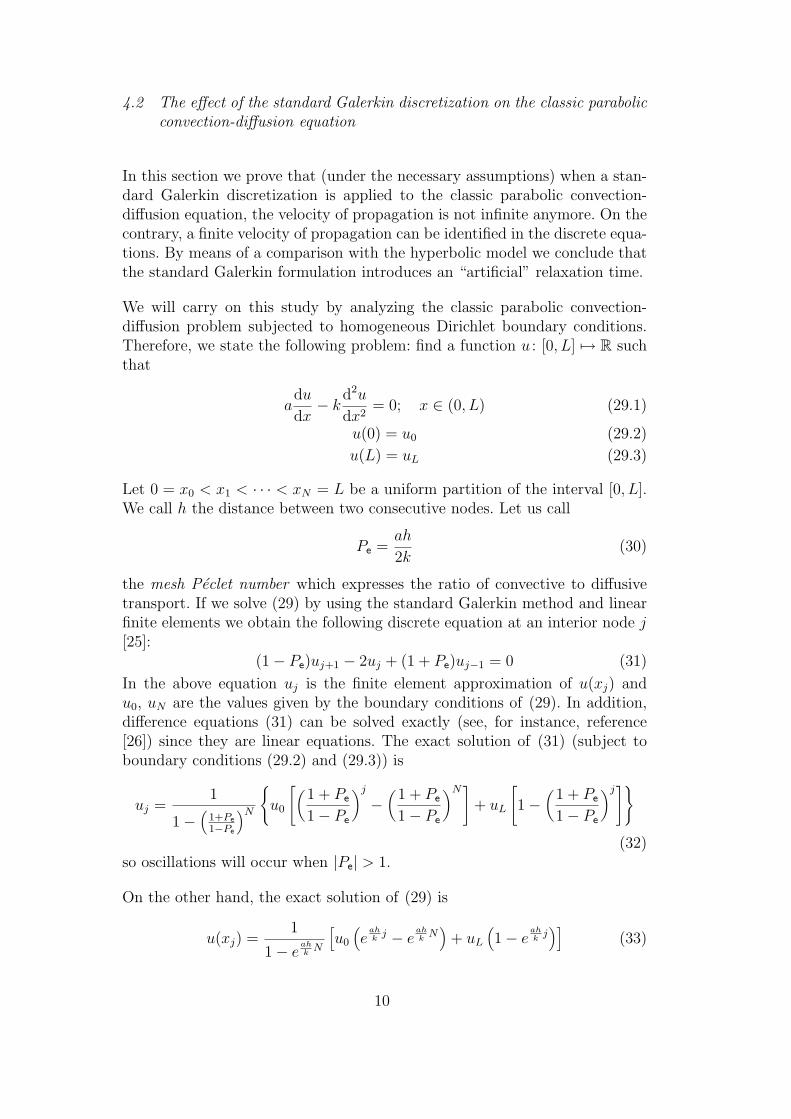
Fig. 1. Dimensionless diffusivity (k?/k) as a function of Pe (left) and dimensionlessnumber H as a function of Pe (right).

A simple comparison between (32) and (33) shows that the approximate so-lution equals the exact one if the following relation holds

e2Pej =(

1 + Pe

1− Pe

)j

∀j = 0, . . . , N (34)

Relation (34) is only satisfied for Pe = 0 (pure-diffusive problem). However,it can be shown that when |Pe| ≤ 1 (i.e. when the mesh is fine enough) theapproximate solution (32) is, in fact, the exact solution of a Cattaneo-typeproblem for a certain relaxation time. To show the former assertion we willprove that (32) is the exact solution of the problem

adu

dx− k? d2u

dx2= 0; x ∈ (0, L) (35.1)

u(0) = u0 (35.2)

u(L) = uL (35.3)

for a certain k? ≤ k. To grant that (32) satisfies (35) the following relationmust be fulfilled:

eahk? j =

(1 + Pe

1− Pe

)j

∀j = 0, . . . , N (36)

We want to obtain k? such that (36) holds. If we admit complex solutions,then k? can always be determined. If we exclusively admit k? to be a realnumber, then (36) has a solution only when |Pe| ≤ 1. The solution of (36) is

k? = k2Pe

ln(

1+Pe

1−Pe

) (37)

By means of (37) we notice that k? → 0 as |Pe| → 1 and k? → k as |Pe| → 0.See figure 1 where k?/k is represented for Pe ∈ (−1, 1). Therefore, the standardGalerkin method applied to (29) solves exactly an underdiffusive equation. On

11

the other hand, equation (37) can be rearranged as

k? = k − k

1− 2Pe

ln(

1+Pe

1−Pe

) < k (38)

If we compare the diffusive coefficient k? with the coefficient which results ofusing Cattaneo’s law (see equation (28)) the following conclusion is achieved:when we solve (29) by using the standard Galerkin method we obtain the solu-tion of a Cattaneo-type transport problem defined by the following relaxationtime:

τG =h

a

1

2Pe− 1

ln(

1+Pe

1−Pe

) (39)

Therefore, an “artificial” relaxation time has been introduced by the Galerkinformulation . As a result, a finite velocity of propagation can be defined in thediscrete equation (31):

cG =a(

1− 2Pe

ln( 1+Pe1−Pe

)

)1/2(40)

By using the relation (40) it is easy to compute the value of “artificial” H (thedimensionless number defined in (19)) for a certain Pe. In figure 1 it has beenrepresented the “artificial” H as a function of Pe. As a result, when we solvethe problem (29) for |Pe| < 1 by using the standard Galerkin method we arereally solving a Cattaneo-type transport problem in subcritical flow conditions.Therefore, we solve a well posed problem because boundary conditions (29.2),(29.3) can be imposed in subcritical flow. However, as |Pe| → 1 the problemwhich is really solved tends to an ill-posed problem.

In what follows we will solve numerically the steady state Cattaneo-type trans-port equation in subcritical and supercritical flow conditions. In order to makeeasier the comparison between the Cattaneo-type transport and the standardformulation of the transport problem we will use equation (28) to describe theproposed model. However, we must take into account that boundary condi-tions that must be imposed are (25.2).

4.3 The standard Galerkin discretization of the hyperbolic model

In this section we will analyze the problem

adu

dx− (k − τa2)

d2u

dx2= 0; x ∈ (0, L) (41.1)

u(0) = u0 (41.2)

u(L) = uL (41.3)

12

which represents a Cattaneo-type transport problem only in subcritical flow.Let us consider again the partition of [0, L] defined by the nodes 0 = x0 <x1 < · · · < xN = L. We call h = L/N .

At this point it is useful to define the dimensionless number

He =ah

2(k − τa2)(42)

which plays a similar role to Pe in the standard description of the transportproblem [13,14]. If we solve (41) by using the standard Galerkin method andlinear finite elements, the following difference equations are found [12]:

(1−He)uj+1 − 2uj + (1 + He)uj−1 = 0; ∀j = 1, . . . , N − 1 (43)

where u0 and uN are given by the boundary conditions (41.2) and (41.3). Inthe same way as (31), difference equations (43) can be solved exactly and thestability condition

|He| ≤ 1 (44)

can be found. If we take τ = 0 in (44) we obtain

|Pe| ≤ 1 (45)

which constitutes a stability condition for the standard formulation. Relations(44) and (45) seem not to be very useful because they can only be applied to(41.1) and (29.1), respectively. However, the asymptotic behavior of (44) isequivalent (except for a scale factor) to impose that the grid step size is smallerthan typical sizes related to the waves which give the solution of the Cattaneo-type transport problem. As we said before, the waves which determine thesolution propagate with celerities a− c and a+ c. Thus, typical sizes upstreamand downstream are τ(c − a) and τ(a + c), respectively. Hence, it is possibleto show [12] that

h < min (τ(c− a), τ(a + c)) (46)

tends to (44) as a tends to the mass wave celerity c, except for a scale factor.

In what follows we will present some numerical solutions of the hyperbolicconvection-diffusion model. For all the examples in section 4 we use a 20(linear) element discretization, L = 1 (thus, h = 0.05) and k = 1.

4.4 Numerical examples in subcritical flow

Now we represent the approximate solution and the exact solution of thehyperbolic convection-diffusion problem. Two groups of numerical exampleswill be presented. At each group the relaxation time is a constant. As we said

13

0 0.1 0.2 0.3 0.4 0.5 0.6 0.7 0.8 0.9 10

0.1

0.2

0.3

0.4

0.5

0.6

0.7

0.8

0.9

1

Spatial coordinate

Concentration

Galerkin-FEMExact

0 0.1 0.2 0.3 0.4 0.5 0.6 0.7 0.8 0.9 1−0.2

0

0.2

0.4

0.6

0.8

1

1.2

Spatial coordinate

Concentration

Galerkin−FEMExact

0 0.1 0.2 0.3 0.4 0.5 0.6 0.7 0.8 0.9 1−0.8

−0.6

−0.4

−0.2

0

0.2

0.4

0.6

0.8

1

Spatial coordinate

Concentration

Galerkin-FEMExact

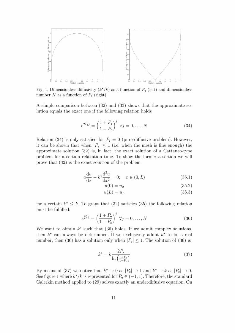
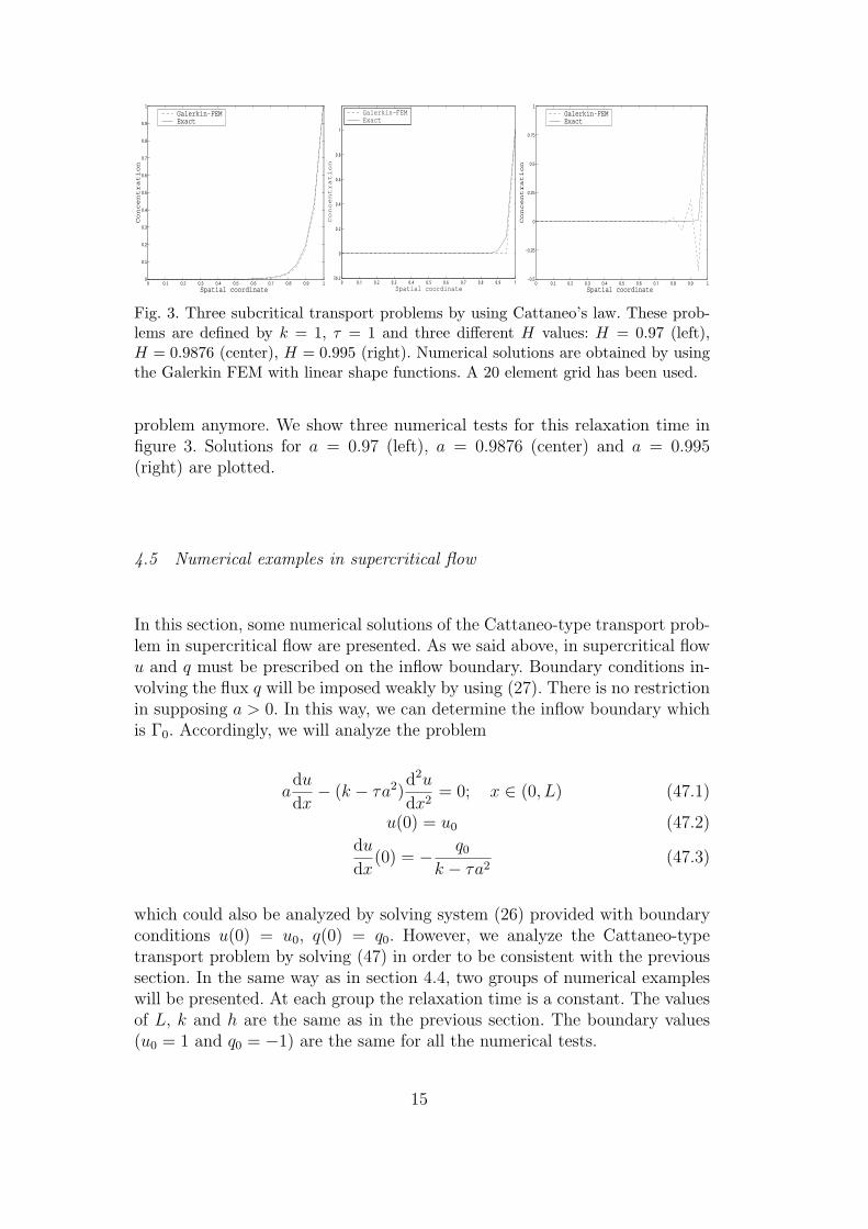
Fig. 2. Three subcritical transport problems by using Cattaneo’s law. These prob-lems are defined by k = 1, τ = 0.01 and three different H values: H = 0.7 (left),H = 0.8828 (center), H = 0.975 (right). Numerical solutions are obtained by usingthe Galerkin FEM with linear shape functions. A 20 element grid has been used.

before, we use a 20 (linear) element mesh, L = 1 (thus, h = 0.05) and k = 1for all examples in section 4. However, at each group we will show three resultsdefined by different fluid velocity values.

4.4.1 Group 1: small relaxation time

This first group of results is defined by τ = 0.01. By using the above values

for k and τ we obtain the diffusive wave celerity c =√

k/τ = 10. Thus, if

|a| ≥ 10, then (41) does not represent a Cattaneo-type transport problemanymore. Our next step will be calculate the maximum a value to obtain astable solution of (41) by using the stability condition |He| ≤ 1. If we do thatwe will see that the numerical scheme used will yield stable solutions when|a| ≤ 8.8278. Therefore, we can say that the numerical solution of (41) isstable for an important range of the possible values of a, because (41) doesnot represent a Cattaneo-type transport problem when |a| ≥ 10.

In figure 2 we show the numerical (dashed line) and the exact (solid line)solutions for three a values. On the left, solutions for a = 7 are plotted. Themiddle graphic shows solutions for a = 8.8278 which is the largest a value thatentails a stable numerical solution. Finally, we plot solutions for a = 9.75 onthe right.

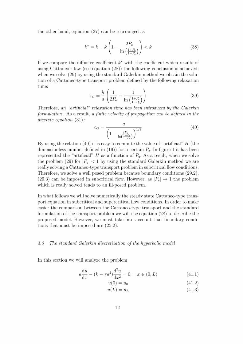
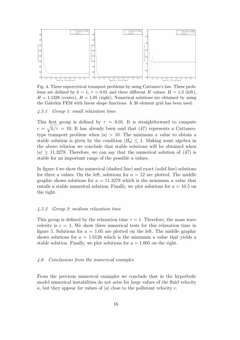
4.4.2 Group 2: medium relaxation time

This group of problems is defined by τ = 1. Therefore, the mass wave celerity

is c =√

k/τ = 1. In addition, according to the stability condition (44), thelargest velocity that entails a stable solution is a = 0.9876. Hence, we willobtain stable solutions if |a| ≤ 0.9876, that is, for almost all possible values ofa because if |a| ≥ 1, then (41) does not represent a Cattaneo-type transport

14

0 0.1 0.2 0.3 0.4 0.5 0.6 0.7 0.8 0.9 10

0.1

0.2

0.3

0.4

0.5

0.6

0.7

0.8

0.9

1

Spatial coordinate

Concentration

Galerkin-FEMExact

0 0.1 0.2 0.3 0.4 0.5 0.6 0.7 0.8 0.9 1−0.2

0

0.2

0.4

0.6

0.8

1

Spatial coordinate

Concentration

Galerkin−FEMExact

0 0.1 0.2 0.3 0.4 0.5 0.6 0.7 0.8 0.9 1−0.5

−0.25

0

0.25

0.5

0.75

1

Spatial coordinate

Concentration

Galerkin-FEMExact

Fig. 3. Three subcritical transport problems by using Cattaneo’s law. These prob-lems are defined by k = 1, τ = 1 and three different H values: H = 0.97 (left),H = 0.9876 (center), H = 0.995 (right). Numerical solutions are obtained by usingthe Galerkin FEM with linear shape functions. A 20 element grid has been used.

problem anymore. We show three numerical tests for this relaxation time infigure 3. Solutions for a = 0.97 (left), a = 0.9876 (center) and a = 0.995(right) are plotted.

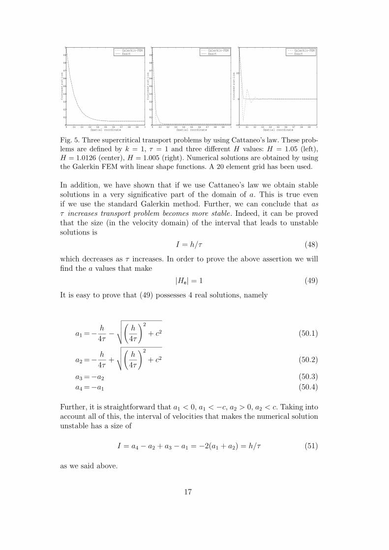
4.5 Numerical examples in supercritical flow

In this section, some numerical solutions of the Cattaneo-type transport prob-lem in supercritical flow are presented. As we said above, in supercritical flowu and q must be prescribed on the inflow boundary. Boundary conditions in-volving the flux q will be imposed weakly by using (27). There is no restrictionin supposing a > 0. In this way, we can determine the inflow boundary whichis Γ0. Accordingly, we will analyze the problem

adu

dx− (k − τa2)

d2u

dx2= 0; x ∈ (0, L) (47.1)

u(0) = u0 (47.2)

du

dx(0) = − q0

k − τa2(47.3)

which could also be analyzed by solving system (26) provided with boundaryconditions u(0) = u0, q(0) = q0. However, we analyze the Cattaneo-typetransport problem by solving (47) in order to be consistent with the previoussection. In the same way as in section 4.4, two groups of numerical exampleswill be presented. At each group the relaxation time is a constant. The valuesof L, k and h are the same as in the previous section. The boundary values(u0 = 1 and q0 = −1) are the same for all the numerical tests.

15

0 0.1 0.2 0.3 0.4 0.5 0.6 0.7 0.8 0.9 10.91

0.92

0.93

0.94

0.95

0.96

0.97

0.98

0.99

1

Spatial coordinate

Co

nce

ntr

atio

n

Galerkin−FEMExact

0 0.1 0.2 0.3 0.4 0.5 0.6 0.7 0.8 0.9 10.91

0.92

0.93

0.94

0.95

0.96

0.97

0.98

0.99

1

Spatial coordinate

Co

nce

ntr

atio

n

Galerkin−FEMExact

0 0.1 0.2 0.3 0.4 0.5 0.6 0.7 0.8 0.9 10.86

0.88

0.9

0.92

0.94

0.96

0.98

1

Spatial coordinate

Co

nce

ntr

atio

n

Galerkin−FEMExact

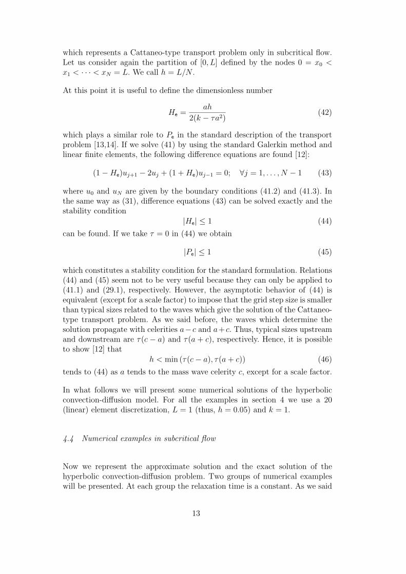
Fig. 4. Three supercritical transport problems by using Cattaneo’s law. These prob-lems are defined by k = 1, τ = 0.01 and three different H values: H = 1.2 (left),H = 1.1328 (center), H = 1.05 (right). Numerical solutions are obtained by usingthe Galerkin FEM with linear shape functions. A 20 element grid has been used.

4.5.1 Group 1: small relaxation time

This first group is defined by τ = 0.01. It is straightforward to compute

c =√

k/τ = 10. It has already been said that (47) represents a Cattaneo-

type transport problem when |a| > 10. The minimum a value to obtain astable solution is given by the condition |He| ≤ 1. Making some algebra inthe above relation we conclude that stable solutions will be obtained when|a| ≥ 11.3278. Therefore, we can say that the numerical solution of (47) isstable for an important range of the possible a values.

In figure 4 we show the numerical (dashed line) and exact (solid line) solutionsfor three a values. On the left, solutions for a = 12 are plotted. The middlegraphic shows solutions for a = 11.3278 which is the minimum a value thatentails a stable numerical solution. Finally, we plot solutions for a = 10.5 onthe right.

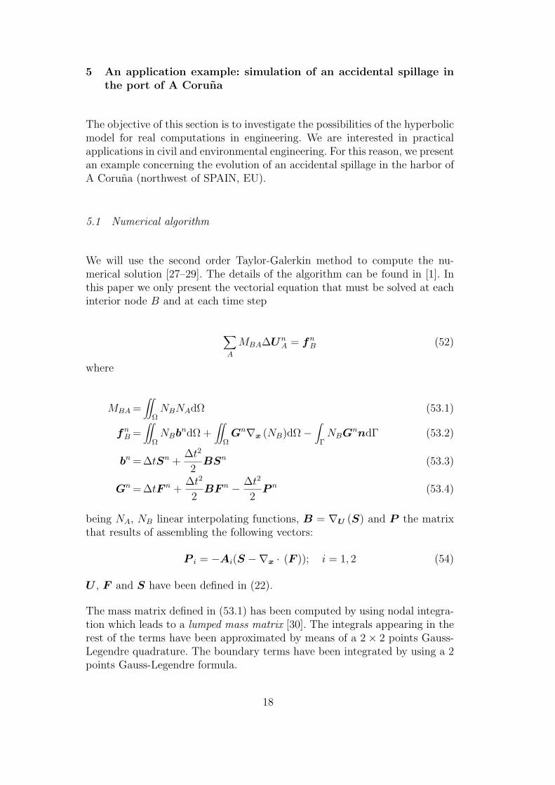
4.5.2 Group 2: medium relaxation time

This group is defined by the relaxation time τ = 1. Therefore, the mass wavecelerity is c = 1. We show three numerical tests for this relaxation time infigure 5. Solutions for a = 1.05 are plotted on the left. The middle graphicshows solutions for a = 1.0126 which is the minimum a value that yields astable solution. Finally, we plot solutions for a = 1.005 on the right.

4.6 Conclusions from the numerical examples

From the previous numerical examples we conclude that in the hyperbolicmodel numerical instabilities do not arise for large values of the fluid velocitya, but they appear for values of |a| close to the pollutant velocity c.

16

0 0.1 0.2 0.3 0.4 0.5 0.6 0.7 0.8 0.9 10

0.1

0.2

0.3

0.4

0.5

0.6

0.7

0.8

0.9

1

Spatial coordinate

Co

nce

ntr

atio

n

Galerkin−FEMExact

0 0.1 0.2 0.3 0.4 0.5 0.6 0.7 0.8 0.9 10

0.1

0.2

0.3

0.4

0.5

0.6

0.7

0.8

0.9

1

Spatial coordinate

Co

nce

ntr

atio

n

Galerkin−FEMExact

0 0.1 0.2 0.3 0.4 0.5 0.6 0.7 0.8 0.9 1−0.5

0

0.5

1

Spatial coordinate

Co

nce

ntr

atio

n

Galerkin−FEMExact

Fig. 5. Three supercritical transport problems by using Cattaneo’s law. These prob-lems are defined by k = 1, τ = 1 and three different H values: H = 1.05 (left),H = 1.0126 (center), H = 1.005 (right). Numerical solutions are obtained by usingthe Galerkin FEM with linear shape functions. A 20 element grid has been used.

In addition, we have shown that if we use Cattaneo’s law we obtain stablesolutions in a very significative part of the domain of a. This is true evenif we use the standard Galerkin method. Further, we can conclude that asτ increases transport problem becomes more stable. Indeed, it can be provedthat the size (in the velocity domain) of the interval that leads to unstablesolutions is

I = h/τ (48)

which decreases as τ increases. In order to prove the above assertion we willfind the a values that make

|He| = 1 (49)

It is easy to prove that (49) possesses 4 real solutions, namely

a1 =− h

4τ−

√√√√( h

4τ

)2

+ c2 (50.1)

a2 =− h

4τ+

√√√√( h

4τ

)2

+ c2 (50.2)

a3 =−a2 (50.3)

a4 =−a1 (50.4)

Further, it is straightforward that a1 < 0, a1 < −c, a2 > 0, a2 < c. Taking intoaccount all of this, the interval of velocities that makes the numerical solutionunstable has a size of

I = a4 − a2 + a3 − a1 = −2(a1 + a2) = h/τ (51)

as we said above.

17

5 An application example: simulation of an accidental spillage inthe port of A Coruna

The objective of this section is to investigate the possibilities of the hyperbolicmodel for real computations in engineering. We are interested in practicalapplications in civil and environmental engineering. For this reason, we presentan example concerning the evolution of an accidental spillage in the harbor ofA Coruna (northwest of SPAIN, EU).

5.1 Numerical algorithm

We will use the second order Taylor-Galerkin method to compute the nu-merical solution [27–29]. The details of the algorithm can be found in [1]. Inthis paper we only present the vectorial equation that must be solved at eachinterior node B and at each time step

∑A

MBA∆UnA = fn

B (52)

where

MBA =∫∫

ΩNBNAdΩ (53.1)

fnB =

∫∫Ω

NBbndΩ +∫∫

ΩGn∇x (NB)dΩ−

∫ΓNBGnndΓ (53.2)

bn = ∆tSn +∆t2

2BSn (53.3)

Gn = ∆tF n +∆t2

2BF n − ∆t2

2P n (53.4)

being NA, NB linear interpolating functions, B = ∇U (S) and P the matrixthat results of assembling the following vectors:

P i = −Ai(S −∇x · (F )); i = 1, 2 (54)

U , F and S have been defined in (22).

The mass matrix defined in (53.1) has been computed by using nodal integra-tion which leads to a lumped mass matrix [30]. The integrals appearing in therest of the terms have been approximated by means of a 2× 2 points Gauss-Legendre quadrature. The boundary terms have been integrated by using a 2points Gauss-Legendre formula.

18

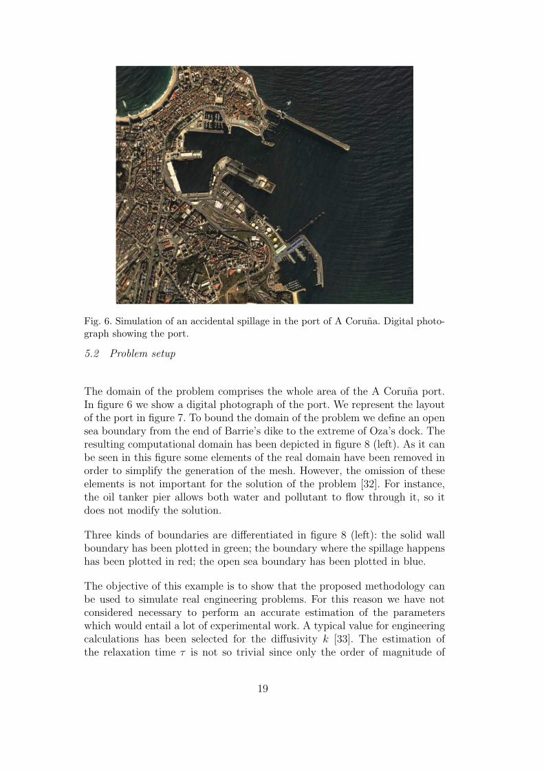
Fig. 6. Simulation of an accidental spillage in the port of A Coruna. Digital photo-graph showing the port.

5.2 Problem setup

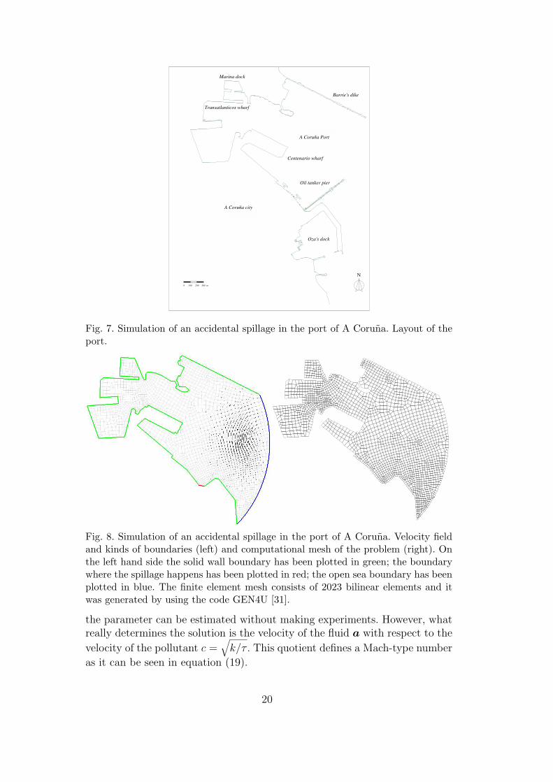
The domain of the problem comprises the whole area of the A Coruna port.In figure 6 we show a digital photograph of the port. We represent the layoutof the port in figure 7. To bound the domain of the problem we define an opensea boundary from the end of Barrie’s dike to the extreme of Oza’s dock. Theresulting computational domain has been depicted in figure 8 (left). As it canbe seen in this figure some elements of the real domain have been removed inorder to simplify the generation of the mesh. However, the omission of theseelements is not important for the solution of the problem [32]. For instance,the oil tanker pier allows both water and pollutant to flow through it, so itdoes not modify the solution.

Three kinds of boundaries are differentiated in figure 8 (left): the solid wallboundary has been plotted in green; the boundary where the spillage happenshas been plotted in red; the open sea boundary has been plotted in blue.

The objective of this example is to show that the proposed methodology canbe used to simulate real engineering problems. For this reason we have notconsidered necessary to perform an accurate estimation of the parameterswhich would entail a lot of experimental work. A typical value for engineeringcalculations has been selected for the diffusivity k [33]. The estimation ofthe relaxation time τ is not so trivial since only the order of magnitude of

19

A Coruña Port

Oza's dock

A Coruña city

Transatlanticos wharf

Marina dock

Barrie's dike

Centenario wharf

Oil tanker pier

N

Fig. 7. Simulation of an accidental spillage in the port of A Coruna. Layout of theport.

Fig. 8. Simulation of an accidental spillage in the port of A Coruna. Velocity fieldand kinds of boundaries (left) and computational mesh of the problem (right). Onthe left hand side the solid wall boundary has been plotted in green; the boundarywhere the spillage happens has been plotted in red; the open sea boundary has beenplotted in blue. The finite element mesh consists of 2023 bilinear elements and itwas generated by using the code GEN4U [31].

the parameter can be estimated without making experiments. However, whatreally determines the solution is the velocity of the fluid a with respect to the

velocity of the pollutant c =√

k/τ . This quotient defines a Mach-type number

as it can be seen in equation (19).

20

Fig. 9. Simulation of an accidental spillage in the port of A Coruna. We show (leftto right and top to bottom) the concentration initial condition and concentrationsolutions at non-dimensional times t∗ = 30, t∗ = 60 and t∗ = 90.

In order to reduce the computations, the velocity field has not been calculated,but it was generated with two constraints: a) it verifies the continuity equationfor incompressible flow and b) it satisfies standard boundary conditions for aviscous flow. The velocity field has been plotted in figure 8 (left). On the righthand side of figure 8 we have depicted the computational mesh.

On the solid wall boundary we impose q ·n = 0. On the boundary where thespillage takes place the condition q · n = −10−2 is imposed. On the open sea

boundary we impose q ·n = cu where c =√

k/τ is the pollutant wave velocity.

The flow is given by H numbers (H = ||a||/c) verifying H ≤ Hmax ≈ 0.3237what makes the problem to be subcritical at each point of the domain. Thecomputation was performed taking a maximum CFL number Cmax ≈ 0.5531.

At this point we define the non-dimensional time t∗ = t/τ . In figure 9 weshow the initial concentration and concentration solutions at non-dimensionaltimes t∗ = 30, t∗ = 60 and t∗ = 90. In figure 10 concentration solutions atnon-dimensional times t∗ = 120, t∗ = 150, t∗ = 300 and t∗ = 1000 are plotted.

21

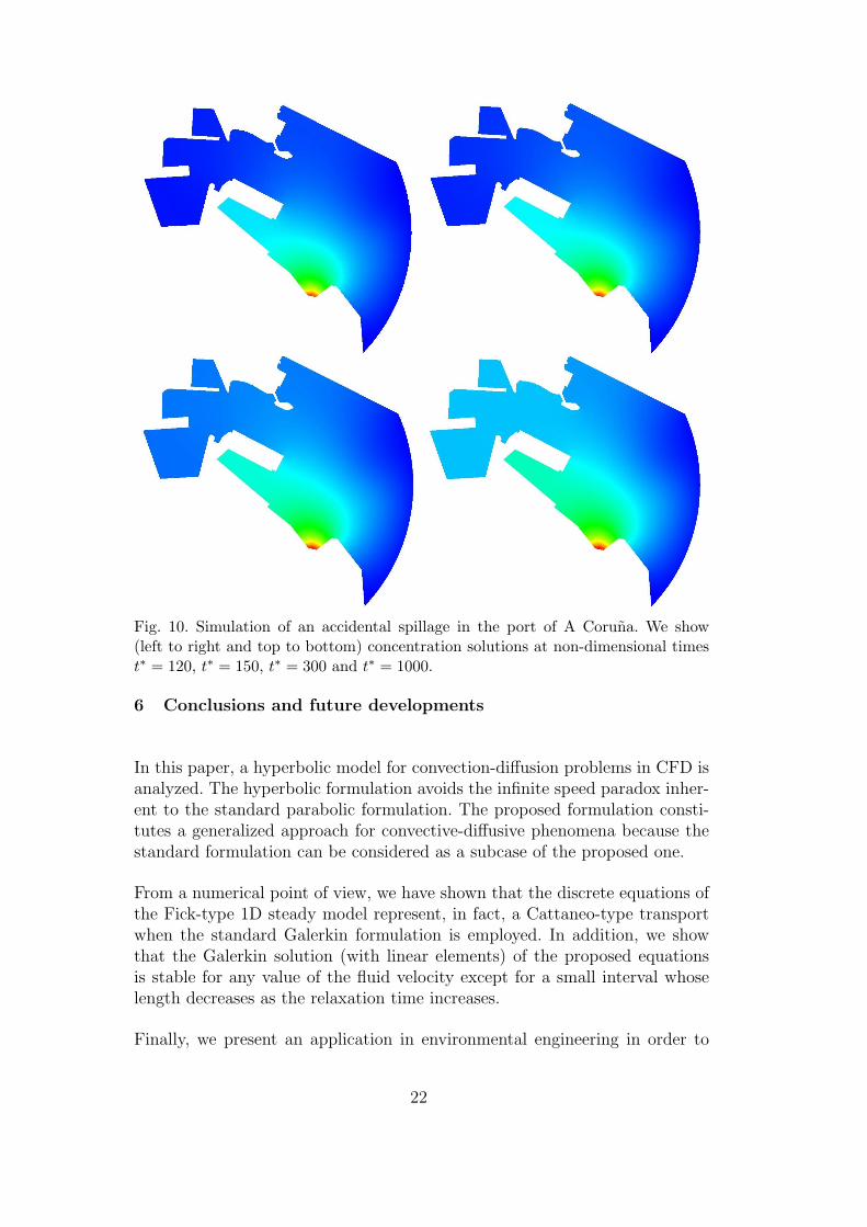
Fig. 10. Simulation of an accidental spillage in the port of A Coruna. We show(left to right and top to bottom) concentration solutions at non-dimensional timest∗ = 120, t∗ = 150, t∗ = 300 and t∗ = 1000.

6 Conclusions and future developments

In this paper, a hyperbolic model for convection-diffusion problems in CFD isanalyzed. The hyperbolic formulation avoids the infinite speed paradox inher-ent to the standard parabolic formulation. The proposed formulation consti-tutes a generalized approach for convective-diffusive phenomena because thestandard formulation can be considered as a subcase of the proposed one.

From a numerical point of view, we have shown that the discrete equations ofthe Fick-type 1D steady model represent, in fact, a Cattaneo-type transportwhen the standard Galerkin formulation is employed. In addition, we showthat the Galerkin solution (with linear elements) of the proposed equationsis stable for any value of the fluid velocity except for a small interval whoselength decreases as the relaxation time increases.

Finally, we present an application in environmental engineering in order to

22

explore the possibilities of the hyperbolic model for real computations. Weconclude that the proposed model is a feasible alternative to the standardparabolic models. However, there are some issues that should be addressed: forexample those concerning the computational cost of the numerical approachand the estimation of the parameters of the model (especially the relaxationtime τ).

7 Acknowledgements

This work has been partially supported by Grant Numbers PGIDT03PXIC18001PNand PGIDT05PXIC18002PN of the “Subdireccion Xeral de I+D de la Xuntade Galicia”, by Grant Numbers DPI2002-00297 and DPI2004-05156 of the“Ministerio de Educacion y Ciencia”, and by research fellowships of the “Uni-versidade da Coruna” and the “Fundacion de la Ingenierıa Civil de Galicia”.

References

[1] H. Gomez, I. Colominas, F. Navarrina, M. Casteleiro, A finite elementformulation for a convection-diffusion equation based on Cattaneo’s law,Computer Methods in Applied Mechanics in Engineering, (2006), in press.

[2] A. Compte, The generalized Cattaneo equation for the description of anomaloustransport processes, Journal of Physics A: Mathematical and General, 30 (1997)7277–7289.

[3] M.N. Ozisik, D.Y. Tzou, On the wave theory in heat conduction, ASME J. HeatTransf., 116 (1994) 526–535.

[4] A. Fick, Uber diffusion, Poggendorff’s Annalen der Physik und Chemie, 94 (1855)59–86.

[5] J.B. Fourier, Theorie analytique de la chaleur, Jacques Gabay, 1822.

[6] M.C. Cattaneo, Sur une forme de l’equation de la chaleur liminant le paradoxed’une propagation instantane, Comptes Rendus de L’Academie des Sciences:Series I-Mathematics, 247 (1958) 431–433.

[7] B. Vick, M.N. Ozisik, Growth and decay of a thermal pulse predicted by thehyperbolic heat conduction equation, ASME Journal of Heat Transfer, 105(1983) 902–907.

[8] Joseph, D.D., Preziosi, L., Heat waves, Reviews of Modern Physics, 61 (1989)41–73.

[9] Joseph, D.D., Preziosi, L., Addendum to the paper “Heat waves”, Reviews ofModern Physics, 62 (1990) 375–391.

23

[10] M. Zakari, D. Jou, Equations of state and transport equations in viscouscosmological models, Physical Review D, 48 (1993) 1597–1601.

[11] T. Ruggeri, A. Muracchini, L. Seccia, Shock waves and second sound in a rigidheat conductor: A critical temperature for NaF and Bi, Physical Review Letters,64 (1990) 2640–2643.

[12] H. Gomez, A new formulation for the advective-diffusive transport problem,Technical Report (in Spanish), University of A Coruna, 2003.

[13] H. Gomez, I. Colominas, F. Navarrina, M. Casteleiro, An alternativeformulation for the advective-diffusive transport problem, 7th Congress onComputational Methods in Engineering, eds. C.A. Mota Soares, A.L. Batista,G. Bugeda, M. Casteleiro, J.M. Goicolea, J.A.C. Martins, C.A.B. Pina, H.C.Rodrigues, Lisbon, Portugal, 2004.

[14] H. Gomez, I. Colominas, F. Navarrina, M. Casteleiro, On the intrinsic instabilityof the advection–diffusion equation, Proc. of the 4th European Congress onComputational Methods in Applied Sciences and Engineering (CDROM), eds. P.Neittaanmaki, T. Rossi, S. Korotov, E. Onate, J. Priaux y D. Knorzer, Jyvaskyla,Finland, 2004.

[15] M. Arora, Explicit characteristic-based high resolution algorithms forhyperbolic conservation laws with stiff source terms, Ph.D. dissertation,University of Michigan, 1996.

[16] G.F. Carey, M. Tsai, Hyperbolic heat transfer with reflection, Numerical HeatTransfer, 5 (1982) 309–327.

[17] H.Q. Yang, Solution of two-dimensional hyperbolic heat conduction by highresolution numerical methods, AIAA-922937 (1992).

[18] M.T. Manzari, M.T. Manzari, On numerical solution of hyperbolic heatequation, Communications in Numerical Methods in Engineering, 15 (1999) 853–866.

[19] Christov, C.I., Jordan, P.M., Heat conduction paradox involving second-soundpropagation in moving media, Physical Review Letters, 94 (2005) 4301-4304.

[20] R. Courant, D. Hilbert, Methods of mathematical physics. Vol II., John Wiley& Sons, 1989.

[21] R. Courant, K.O. Friedrichs, Supersonic flow and shock waves, Springer Verlag,1999.

[22] G.B. Whitham, Linear and nonlinear waves, John Wiley & Sons, 1999.

[23] F. Alcrudo, Total variation diminishing high-resolution schemes for free surfaceflows, PhD dissertation (in Spanish), University of Zaragoza, 1992.

[24] H. Gomez, A hyperbolic formulation for convective-diffusive problems in CFD,Ph.D. dissertation (in Spanish), University of A Coruna, 2006.

24

[25] R. Codina, A finite element formulation for the numerical solution of theconvection-diffusion equation, Technical Report 14, International Center forNumerical Methods in Engineering (CIMNE), 1993.

[26] E. Isaacson, H.B. Keller, Analysis of numerical methods, John Wiley & Sons,1966.

[27] J. Donea, A Taylor-Galerkin method for convective transport problems,International Journal for Numerical Methods in Engineering, 20 (1984) 101–120.

[28] J. Donea, L. Quartapelle, V. Selmin, An analysis of time discretization in thefinite element solution of hyperbolic problems, Journal of Computational Physics,70 (1987) 463–499.

[29] J. Donea, L. Quartapelle, An introduction to finite element methods fortransient advection problems, Computer Methods in Applied Mechanics andEngineering, 95 (1992) 169–203.

[30] T.J.R. Hughes, The finite element method. Linear static and dynamic finiteelement analysis, Dover Publications, 2000.

[31] J. Sarrate, A. Huerta, Efficient unstructured quadrilateral mesh generation,International Journal for Numerical Methods in Engineering, 49 (2000) 1327–1350.

[32] C.A. Figueroa, I. Colominas, G. Mosqueira, F. Navarrina, M. Casteleiro, Astabilized finite element approach for advective-diffusive transport problems,Proceedings of the XX Iberian Latin-American Congress on ComputationalMethods in Engineering (CDROM), eds. P.M. Pimenta, R.Brasil, E.Almeida,Sao Paulo, Brasil, 1999.

[33] E.R. Holley, Diffusion and Dispersion, Environmental Hydraulics, 111-151, V.P.Singh and W.H. Hager (Eds.), Kluwer: Dordrecht, 1996.

25