A HYBRID ALGORITHM FOR THE ONE MACHINE SEQUENCING PROBLEM TO MINIMIZE TOTAL TARDINESS*

V. Srinivasan

The University of Rochester Rochester, New York

ABSTRACT

In a recent paper, Hamilton Emmons has established theorems relating to the order in which pairs of jobs are to be processed in an optimal schedule to minimize the total tardiness of performing n jobs on one machine. Using these theorems, the algorithm of this paper determines the precedence relationships among pairs of jobs (whenever possible) and eliminates the first and the last few jobs in an optimal sequence. The remaining jobs are then ordered by incorporating the precedence relationships in a dynamic programming framework. Propositions are proved which considerably reduce the total computation in- volved in the dynamic programming phase. Computational results indicate that the solution time goes up less than linearly with the size (n) of the problem. The median solution time for solving 50 job problems was 0.36 second on UNIVAC 1108 computer.

I. INTRODUCTION The one-machine sequencing problem to minimize total tardiness may be stated as follows: We are given a set of jobs { 1, 2, . . ., n ) whose sequence-independent processing times PI, pn,

. . ., pn and due dates d l , di , . . ., d , are known. The jobs are available simultaneously at time zero and are to be sequenced on one machine. The set-up times are independent of the sequence and conse- quently are assumed to be included in the processing times.

Let {(l), (2), . . ., (n)} be a permutation of the integers { 1,2, . . ., n} denoting a particular sequence of the n jobs. (Thus (2)=4 if the fourth job is scheduled second.) The completion time of the (i)th job c(i)=p(,)+p(2)+. . . +p(i) and its lateness l ( ~ = c ( i ) - d ( i ) . Minimizing total lateness may not be a good objective since it gives equal credit for finishing a job early as it penalizes for finishing a job late. Tardiness considers only positive lateness (jobs which are not completed by their due dates) i.e., t ( i )

= max [ l ( i ) , 01 so that minimizing total tardiness may be a more desirable objective in many situations. Thus for a sequence {(l), (2), . . ., (n)} the total tardiness T is given by

(1) T=max [O , ( P ( ~ - d ~ ~ ) l + m a x [O , (pc1)+~(2) -42) l l +- - -+max [ O , @ ( U + P ( ~ + - - -+~(n) - -n) ) ]

The objective is to find a sequence that minimizes T. Other reasons for using T rather than other meas- ures of performance are discussed in [2].

11. PREVIOUS RESEARCH For the general case, where no restrictive assumptions are imposed on the processing times and

due dates, several algorithms have been proposed for minimizing total tardiness [H, 8-10]. The algorithm of Schild and Fredman [9] cannot guarantee optimality [3] and no computational results have

*This report was prepared when the author was a member of the Management Sciences Research Group, Camegie-Mellon University. Reproduction in whole or in part is permitted for any purpose of the U S . Government.

317

318 V. SRINIVASAN

been published about the quality of the solution. The network algorithm due to Elmaghraby [4], which a significant improvement over complete enumeration, is laborious and applicable only to smaller problems. A dynamic programming formulation for the general case of nonlinear loss functions has been given by Held and Karp [6], Lawler [8], and Schild and Fredman [lo]. Computer memory requirements restrict the size of the problem that can be handled by this formulation, for example, the maximum problem that could be solved on the IBM 7090 is 13 jobs without resorting to any bulk storage [6].

In Ref. [5] Emmons has proved theorems that establish the relative order in which pairs of jobs are processed in an optimal schedule. If for some pair(s) of jobs the conditions of the theorems are not satisfied, then one obtains only a partial order of the jobs in the optimal sequence. If, for instance, nothing is known about the relative order of the jobs ( i , j) then Emmons suggests branching into two subproblems by assuming i precedes j and vice versa. For a large problem, the size of tree so obtained can quickly get out of hand. Since no computational results are available for Emmons' algorithm it could not be compared with the present one.

111. THE HYBRID ALGORITHM The algorithm proposed in this paper is hybrid in the sense that it incorporates theoretical results

into the dynamic programming framework to reduce the total computational effort.

Outline of the Algorithm: PHASE 1: Jobs which have excessively long due dates (to be defined shortly) are directly identified

as the last jobs in an optimal sequence. PHASE 2: Theorems 1 and 2 of Emmons [5] are repeatedly used to obtain as many precedence

relationships among the jobs as possible. In general, the first and the last few jobs of the optimal se- quence can be directly identified in this process.

PHASE 3: The remaining jobs are ordered by incorporating the precedence relationships in a dynamic programming framework [6,8, 101 modified to take into account the precedence relationships determined in phase 2.

Detailed Description of Phases 1,2, and 3:

PHASE 1: If di > P = $' pj , then there exists an optimal schedule in which i is processed last j= 1

[5, p. 7031. The result is obvious since by the property that di > P, job i is never tardy in any sequence and

hence can safely be sequenced last. In doing so, P is reduced to P - p i and another job may become eligible for removal as the last job among the remaining n- 1 jobs. After repeating this procedure as many times as possible, we update n to be the remaining number of jobs.*

PHASE 2: Hereafter we will assume that the n remaining jobs are arranged in the order of non- decreasing processing times ( p , c pz, . . ., c p n ) and in the case of equality, in the order of non- decreasing due dates. Thus i < j implies pi < p, or pi=pj and di dj. Let N be the set of jobs { 1,2, . . . , n} arranged in that order.

*If at any stage, there are k jobs (k > 1) which satisfy this elimination criterion, then one can arbitrarily choose any one of them to be the last. The remaining (k- 1) of these jobs will get eliminated in successive stages. The order is not important since each of these jobs should have zero tardiness in the optimal sequence.

ONE MACHINE SEQUENCING 31% We use the notation i + j which may be read as “i precedes j” to mean that there exists an

optimal schedule in which i precedes j. Let Ai and Bi be the sets of indices of all jobs that at any point in the algorithm have been shown to come after and before i, respectively. We will denote the number of jobs in a set S as IS(.

To keep track of the precedence relationships, we introduce the notion of a Precedence Matrix M (of size n x n) where mjj= I if i + j and m,j=O otherwise. The diagonal elements mii of this matrix do not have any significance and are marked ‘-’. By definition, At= {jlmij= 1) and Bi= {j\mji= 1). Thus /Ail will be given by the number of 1’s in the ith row and IBil will be given by the number of 1’s in ith column of the matrix M.

For convenience of the reader Ernrnons’ Theorems 1 and 2 are restated below using the notatiod of the precedence matrix. Computational results revealed that the additional precedence relationships obtained by applying Ernmons’ Theorem 3 were negligible and hence this theorem was not used.

THEOREM 1: For any two jobs j and k withj < k , if dj 6 rnax (pk + THEOREM 2: For any two jobs j and k with j < k , if dj >max (&+

2 p i , dk) , then mjk = 1.

2 pr, 4) and

i h k = l

i \mik= 1

dj+pj 2 p i , then mkj= 1. ilmki=O

We first apply Theorems 1 obtained, then reapplication of

and 2 to all pairs (j, k) withj < k. If any precedence relationships are the theorems may generate additional precedence relationships. This

iterative process terminates when no new precedence relationships are obtained in a particular iteration. Any theorems regarding precedence relationships that may subsequently become known could be

readily built into this framework provided they result in net computational gain. It is obvious that if lAil= n - 1 then i is clearly the first job in the optimal sequence. Thus i can be

removed from the set N and n redefined as n - 1. The due dates of the jobs in the set N become dj-pi to account for the fact that i has already been scheduled. Similarly, if lBil= n- 1, i is sequenced last, and N and n are accordingly redefined. Whenever a job is identified as either first or last, additional precedence relationships may be generated by reapplying Theorems 1 and 2.

PHASE 3: We first describe the well known dynamic programming approach to this problem [6,8, 101 and then state some propositions which will considerably reduce the computation involved.

Let J denote any set of k jobs scheduled last. Let s(J) denote the “Earliest Start Time” of the jobs in J i.e., s(J)=z pi, where J = N - J denotes the first (n- k) jobs. Bellman’s Principle of Optimality [l]

may now be stated: If the schedule is optimal, it has the property that regardless of the order in which the first n-k jobs are performed, the remainder of the schedule constitutes an optimal schedule of the subset of jobs J subject to the restriction that none of the jobs are commenced before s(&.

Let T(J) denote the minimum total tardiness of performing the jobs in J subject to the restriction that no job in J is commenced before s(J).

To obtain the recursive relation of the dynamic programming formulation we reason as follows: T ( J J i ) , the minimum tardiness of J given that { i} is sequenced first among the jobs in J , is:

,J

320 V. SRINIVASAN

Here the first term denotes the contribution to total tardiness of job {i} and the second term gives the minimum tardiness of the remaining jobs in J . Removing the condition on { i} , we get

where T(+)=O for the empty set 4. The recurrence relation (3) is to be repeated for IJI=l, 2, . . ., n to obtain the optimal solution.

At the kth stage (i.e., I J I = k ) one would normally evaluate T ( J ) for all the (g) combinations of jobs. We now prove three propositions which considerably reduce this number of evaluations.

PROPOSITION 1: Let R = {i: IAi( 2 k } . Let N I = N - R . Then for the kth stage optimization one need consider only the n l jobs in N1.

PROOF: /Ail 2 k , by definition, means that there exists an optimal schedule in which i precedes at least k jobs. Thus i need not be considered for the kth stage optimization.

PROPOSITION 2: Let Q = { i: [Ail = k- l}. Let N , =N1- Q contain n2 jobs. Then in the set of J’s in which i appears, one need consider only that]= {i} U Ai for the kth stage. Furthermore

PROOF: /All = k- 1 implies that there exists an optimum schedule in which i precedes the k- 1 jobs in A,. Thus {i} is the first job in the optimal schedule for J so that T ( J ) = T ( J ( i ) . Eq. (4) directly follows from (2) since J - { i} = Ai.

As a result of the above two propositions the total number of combinations for the kth stage are reduced from (1) to ($2 ) + (nl -n2) . Proposition 3 below further reduces this number.

PROPOSITION 3: Let i be a job, such that mij = 1 for j = il, ‘iz, , . ., il; I < k - 1. Then in the set of J’s in which i appears, one need choose only those in which i appears together with jobs il, i p , . . ., il.

PROOF: The proof of this proposition is similar to that of Proposition 2. We now consider the functional equation, Eq. (3), where for a given J, one would normally have to

evaluate all the k alternatives for the first job in J. Proposition 4 below reduces this number of evaluations.

PROPOSITION 4: Let L = {i:lBtl 2 n - k + 1). Then only the jobs in N3 = N - L need be con- sidered as candidates for the first job of the kth stage optimization for].

PROOF: (B,( 3 n - k + 1 means that there is an optimal schedule in which at least n - k + 1 jobs precede i ; i.e., i is one of the last (k - 1) jobs in the optimal schedule. Hence i need not be con- sidered for the first position in a k job problem. Thus all potential candidates for the first job are in N3 = N - L . Using this result we may rewrite (3) as

ONE MACHINE SEQUENCING 321

Jobname

P

d

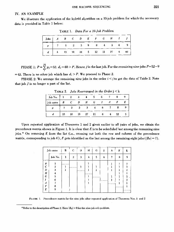
IV. AN EXAMPLE We illustrate the application of the hybrid algorithm on a 10-job problem for which the necessary

data is provided in Table 1 below:

B C D H G I A F E

1 2 3 3 4 6 7 8 9

13 10 10 27 11 6 4 12 5

TABLE 1. Data For a 10-Job Problem

d 4 13 10 10 12 11 27 6 60

Job name B

Job No. 1

B 1 ......... C 2 1 D 3 1 H 4 G 5 I 6 A 7 F 8 E 9

10

PHASE 1: P = C pj =52. dJ = 60 > P. Hence Jis the last job. For the remaining nine jobs P=52-9 1

=43. There is no other job which has di > P. We proceed to Phase 2.

that job J is no longer a part of the list. PHASE 2: We arrange the remaining nine jobs in the order i < j to get the data of Table 2. Note

C D H G

2 3 4 5

1 ......... 1 1 1

......... 1 1 .........

1 ........ 1 1

TABLE 2. Jobs Rearranged in the Qrder j < k

........

JobNo. 1 1 2 3 4 5 6 7 8 9 I

I A F E

6 7 8 9

1 1 1 1 1 1 1 1 1

1 1 1 1 1 , 1 1 1

......... 1 1 ......... 1

........

Upon repeated application of Theorems 1 and 2 given earlier to all pairs of jobs, we obtain the precedence matrix shown in Figure 1. It is clear that E is to be scheduled last among the remaining nine jobs.* On removing E from the list (i.e., crossing out both the row and column of the precedence matrix, corresponding to job E), F gets identified as the last among the remaining eight jobs ( JBFI = 7).

FILURE 1. Precedence matrix for the nine jobs after repeated application of Theorems Nos. 1 and 2

*Refer to the description of Phase 2. Here ( B E ( = 8 for the nine-job sub problem.

322 V. SRINIVASAN

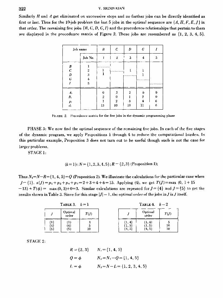
Similarly H and A get eliminated on successive steps and no further jobs can be directly identified as first or last. Thus for the 10-job problem the last 5 jobs in the optimal sequence are {A, H, F, E, J } in that order. The remaining five jobs {B, C, D, G, I } and the precedence relationships that pertain to them are displayed in the precedence matrix of Figure 2. These jobs are renumbered as (1, 2, 3, 4, 5).

FILURE 2. Precedence matrix for the five jobs in the dynamic programming phase

PHASE 3: We now find the optimal sequence of the remaining five jobs. In each of the five stages of the dynamic program, we apply Propositions 1 through 4 to reduce the computational burden. In this particular example, Proposition 3 does not turn out to be useful though such is not the case for larger problems.

STAGE 1:

(A= 1): N = { 1,2,3,4,5}; R = {2,3} (Proposition 1);

Thus Nl=N-R={ 1 ,4 ,5}=Q (Proposition 2). We illustrate the calculations for the particular case when

- 13) + T ( # ) = max (0, 3)+0=3. Similar calculations are repeated for J = (4) and J = (5) to get the results shown in Table 3. Since for this stage I J I = 1, the optimal order of the jobs inJ isJ itself.

J = { l } . s ( / ) = p , + p s + p 4 + p 3 = 2 + 3 + 4 + 6 = 1 5 . Applying (4), we get T(J)=max (0, 1+15

TABLE 3. k = 1 r

STAGE 2:

TABLE 4. k = 2

T ( J ) Optimal order J

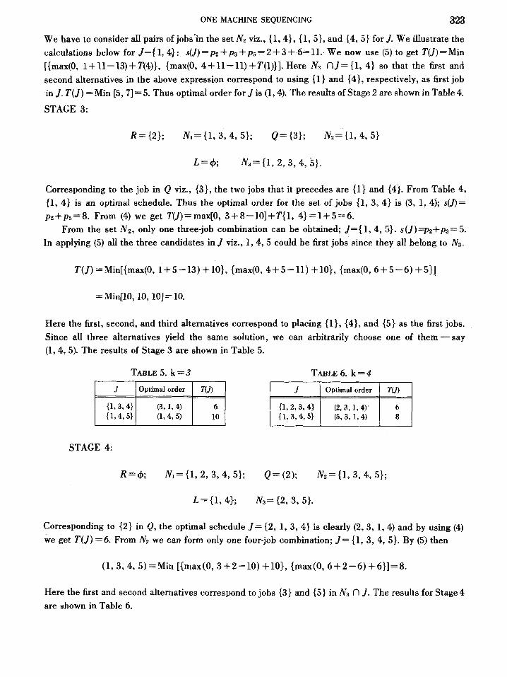
ONE MACHINE SEQUENCING 323 We have to consider all pairs of jobs'in the set NZ viz., (1,4), (1, 5), and (4, 5) for J. We illustrate the calculations below for J={1,4}: s(J)=pZ+p3+p5=2+3+16=11. We now use (5) to get T(J)=Min [(max(O, 1+11-13)+7'(4)}, (max(0, 4+11-11)+7'(1)}]. Here N3 nJ=(1 , 4) so that the first and second alternatives in the above expression correspond to using (1) and {4), respectively, as first job in J . T ( J ) = Min [5,7]=5. Thus optimal order for J is (1,4). The results of Stage 2 are shown in Table 4.

STAGE 3:

R=(2}; NI={l, 3, 4, 5); Q=(3); Nz=(l, 4, 5}

Corresponding to the job in Q viz., {3), the two jobs that it precedes are (1) and (4). From Table 4, (1, 4) is an optimal schedule. Thus the optimal order for the set of jobs (1 ,3 ,4} is (3, 1, 4); s(J)= pz+p5=8 . From (4) we get T(J)=max[O, 3+8--10]+T(1, 4)=1+5=6.

From the set Nz, only one three-job combination can be obtained; J = ( 1, 4, 5). s (J)=pz+ps= 5. In applying (5) all the three candidates in J viz., 1 , 4 , 5 could be first jobs since they all belong to N3.

T ( J ) =Min[(max(O, 1+5-13) +lo), {max(O, 4+5-11) +lo}, {max(O, 6+5-6) +5)]

= Min[lO, 10, 101 = 10.

Here the first, second, and third alternatives correspond to placing (l), {4), and (5) as the first jobs. Since all three alternatives yield the same solution, we can arbitrarily choose one of them-say (1,4, 5). The results of Stage 3 are shown in Table 5.

STAGE 4:

L = (1, 4); N3= (2, 3, 5).

Corresponding to (2) in Q, the optimal schedule J = (2, 1, 3, 4) is clearly (2, 3, 1 ,4) and by using (4) we get T ( J ) =6. From Nz we can form only one four-job combination; J = { 1, 3, 4, 5). By (5) then

(1, 3, 4, 5) =Min [(max(O, 3+2-10) +lo>, (max(0, 6+2-6) +6)]=8.

Here the first and second alternatives correspond to jobs (3) and (5) in N3 f l J . The results for Stage 4 are shown in Table 6.

324

STAGE 5:

V. SRINIVASAN

J f l N3 = (2,s) so that by applying (5) we obtain

T(J)=Min [{max(O, 2-10) + 8 } , {max(O, 6 - 6 ) + 6 } ] = 6 .

‘Thus the optimal sequence for the five-job problem= (5, 2 , 3, 1,4} = { I C D B G}. Thus the optimal sequence for the 10-job problem is { I C D B G A H F E J } with a total tardiness of 85.

V. COMPUTATIONAL RESULTS The algorithm of Section I11 was coded* in Fortran V and tested with a number of randomly

generated problems using the UNIVAC 1108. The results are very promising; however, at this point there are no computational results for the other algorithms [4, 5 , 6 , 8 , 9 , 101 available for comparison.

The processing times and the due dates were drawn from a bivariate normal distribution con- fined to the positive quadrant. The distribution is completely specified by mean processing time and due date p p and pd, their standard deviations s , ~ and Sd, and the correlation coefficient p. To randomly draw a job characterized by (F, d), we use the well known fact that the conditional distribution of d given p is also normal with mean pd+ (p Sd/sp) (F - p,,) and standard deviation sd ( 1 - p2)112.

To study the effect of the parameters on the solution time, a series of 12 job problems were run using different values for the parameters. Since multiplying the processing times and due dates by an arbitrary constant does not affect the optimal schedule, we can arbitrarily fix one of the parameters- p,l was set equal to 10 for all problems.

The value of pd may be decided by t, the “tardiness” of the shop-a measure of the fraction of the jobs that are completed beyond their due dates. Thus if n is the number of jobs to be scheduled, roughly n(1-t) jobs will be completed by their due ,dates- the n(1-t)th job’s completion time n(l-t)pp (on an average) and its due date pd (on an average) will be roughly equal. Hence

The standard deviations sI, and S d can be more conveniently conceptualized by their coefficients of variation s, /pp and Sdlp&

The experimental set-up was a 34 factorial design [7], i.e., each of the four parameters could take any one of three values given below (as mentioned already, n=12 and pp=lO).

(a) Mean due date pd=30,60,90 (t=0.75, 0.5, 0.25)

(b) Coefficient of variation sll~p,=0.20, 0.50, 0.80

*This computer program was written by Mr. Nathaniel F. Tarbox, and the author.

ONE MACHINE SEQUENCING

(c) Coefficient of variation sd/pd=0.20, 0.50, 0.80

325

(4 Coefficient of correlation p=- 0.7,0,0.7

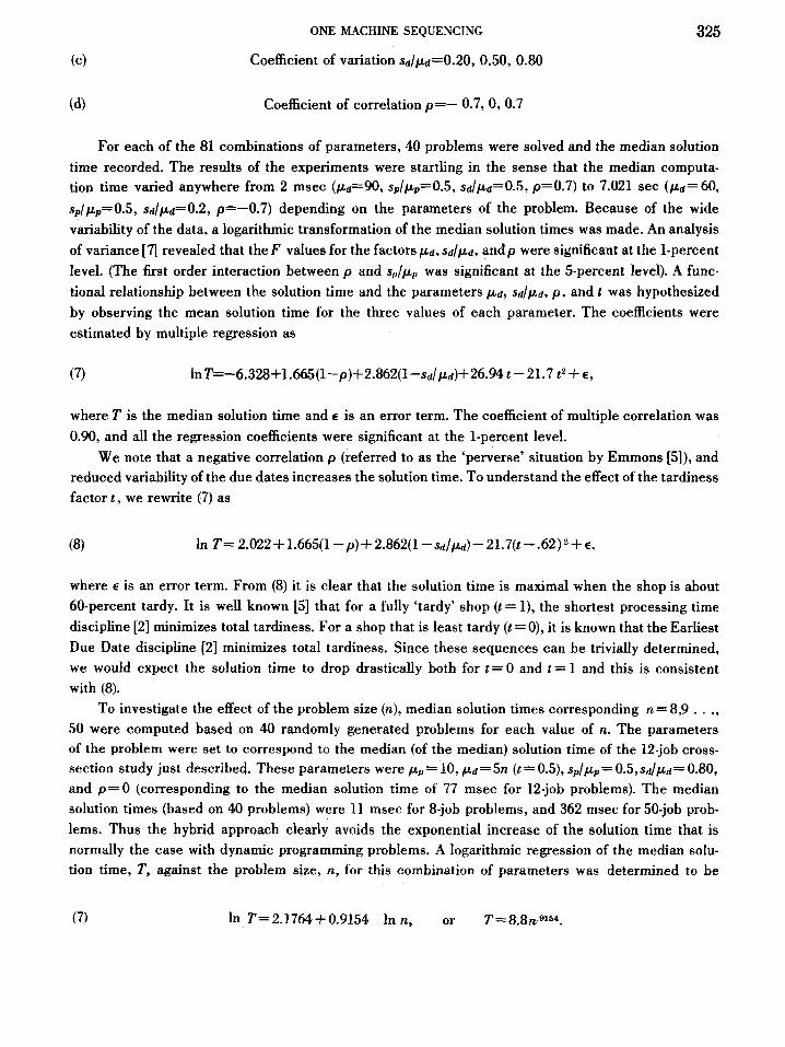
For each of the 81 combinations of parameters, 40 problems were solved and the median solution time recorded. The results of the experiments were startling in the sense that the median computa- tion time varied anywhere from 2 msec (pd=90, splpp=0.5, sd/pd=o& p=0.7) to 7.021 sec (pd=60, sp/pp=0.5, sd/pd=o.2, p=-0.7) depending on the parameters of the problem. Because of the wide variability of the data, a logarithmic transformation of the median solution times was made. An analysis of variance [A revealed that t h e F values for the factors p d , sd/pd, andp were significant at the 1-percent level. (The first order interaction between p and sI,/pp was significant at the 5-percent level). A func- tional relationship between the solution time and the parameters p d , sd/pd, p , and t was hypothesized by observing the mean solution time for the three values of each parameter. The coefflcients were estimated by multiple regression as

where T is the median solution time and E is an error term. The coefficient of multiple correlation was 0.90, and all the regression coefficients were significant at the 1-percent level.

We note that a negative correlation p (referred to as the ‘perverse’ situation by Emmons [5]), and reduced variability of the due dates increases the solution time. To understand the effect of the tardiness factor t , we rewrite (7) as

(8) In T= 2.022+ 1.665(1 -p)+ 2.862(1 -Sd/&$)- 21.7(t - .62)’+ E,

where E is an error term. From (8) it is clear that the solution time is maximal when the shop is about 60-percent tardy. It is well known [5] that for a fully ‘tardy’ shop (t= l ) , the shortest processing time discipline [2] minimizes total tardiness. For a shop that is least tardy (t = 0), it is known that the Earliest Due Date discipline [2] minimizes total tardiness. Since these sequences can be trivially determined, we would expect the solution time to drop drastically both for t = 0 and t = 1 and this is consistent with (8).

To investigate the effect of the problem size (n), median solution times corresponding n=8,9 . . ., 50 were computed based on 40 randomly generated problems for each value of n. The parameters of the problem were set to correspond to the median (of the median) solution time of the 12-job cross- section study just described. These parameters were p p = lo, pd=5n (t= 0.5), sp/pp=o.5,sd/pd= 0.80, and p=O (corresponding to the median solution time of 77 msec for 12-job problems). The median solution times (based on 40 problems) were 11 msec for 8-job problems, and 362 msec for 50-job prob- lems. Thus the hybrid approach clearly avoids the exponential increase of the solution time that is normally the case with dynamic programming problems. A logarithmic regression of the median solu- tion time, T, against the problem size, n, for this combination of parameters was determined to be

t 7) In T=2.1764+0.9154 In n, or T=8.8n.9154.

V. SRINIVASAN 326 Thus the solution time goes up less than linearly with the size of the problem. (The correlation coeffi- cient was 0.8852 and the two regression coefficients were significant at the 0.1-percent level.)

Core limitations prevented the testing of larger problems which would have needed auxiliary storage like drums, discs, or tapes. It is important to note that all the results reported above were median solution times. Even in the 12-job cross-sectional study, 40 out of the 3,240 problems (81 X 40) were not fully solved because they took longer than 1 min. One may well state that the solution times belong to some infinite variance distribution (For the 12-job problems, the times varied anywhere between 1 msec to more than 1 min).

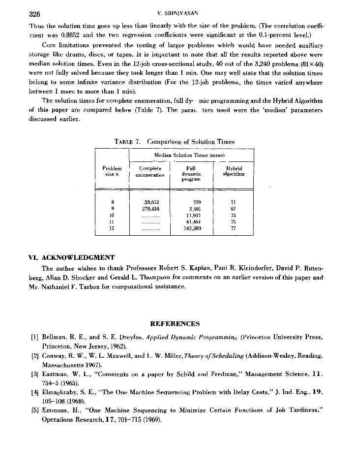
The solution times for complete enumeration, full dyl mic programming and the Hybrid Algorithm of this paper are compared below (Table 7). The parai. ters used were the ‘median’ parameters discussed earlier.

Problem size n

a 9

10 11 12

TABLE 7. Comparison of Solution Times

Median Solution Times (msec) I Complete Full Hybrid

enumeration dynamic algorithm program

28,652 709 11

........... 11,931 73

........... 41,461 75

........... 143,580 77

2 7 8 , ~ ~ 2,481 67

I I I I t

VI. ACKNOWLEDGMENT The author wishes to thank Professors Robert S. Kaplan, Paul R. Kleindorfer, David P. Ruten-

berg, Allan D. Shocker and Gerald L. Thompson for comments on an earlier version of this paper and Mr. Nathaniel F. Tarbox for computational assistance.

REFERENCES

[l] Bellman, R. E., and S. E. Dreyfus, Applied Dynamic Programming (Princeton University Press,

[2] Conway, R. W., W. L. Maxwell, and L. W. Miller, Theory ofScheduling (Addison-Wesley, Reading,

[3J Eastman, W. L., “Comments on a paper by Schild and Fredman,” Management Science, 11,

[4] Elmaghraby, S. E., “The One Machine Sequencing Problem with Delay Costs,” J. Ind. Eng., 19,

[S] Emmons, H., “One Machine Sequencing to Minimize Certain Functions of Job Tardiness,”

Princeton, New Jersey, 1962).

Massachusetts 1967).

75475 (1965).

105-108 (1968).

Operations Research, 17,701-715 (1969).

ONE MACHINE SEQUENCING 327

[6] Held, M., and R. M. Karp, “A Dynamic Programming Approach to Sequencing Problems,”

[q Kempthorne, O., The Design and Analysis of Experiments (John Wiley and Sons, Inc., New York,

[8] Lawler, E. L., “On Scheduling Problems with Deferral Costs,” Management Science, 11,280-288

[9] Schild, A., and I. J. Fredman, “On Scheduling Tasks with Associated Linear Loss Functions,”

[ 101 Schild, A., and I. J. Fredman, “Scheduling Tasks with Deadlines and Nonlinear Loss Functions,”

SIAM J., 10,196-210 (1962).

1952).

(19a).

Management Science, 7,280-285 (1961).

Management Science, 9, 73-81 (1962).