a high-resolution scheme for low mach number flows
TRANSCRIPT
INTERNATIONAL JOURNAL FOR NUMERICAL METHODS IN FLUIDSInt. J. Numer. Meth. Fluids 2004; 46:245–261 (DOI: 10.1002/�d.741)
A high-resolution scheme for low Mach number �ows
Saugata Chakravorty and Joseph Mathew∗;†
Department of Aerospace Engineering; Indian Institute of Science; Bangalore 560 012; India
SUMMARY
A method for computing low Mach number �ows using high-resolution interpolation and di�erenceformulas, within the framework of the Marker and Cell (MAC) scheme, is presented. This increasesthe range of wavenumbers that are properly resolved on a given grid so that a su�ciently accuratesolution can be obtained without extensive grid re�nement. Results using this scheme are presented forthree problems. The �rst is the two-dimensional Taylor–Green �ow which has a closed form solution.The second is the evolution of perturbations to constant-density, plane channel �ow for which linearstability solutions are known. The third is the oscillatory instability of a variable density plane jet. Inthis case, unless the sharp density gradients are resolved, the calculations would breakdown. Under-resolved calculations gave solutions containing vortices which grew in place rather than being convectedout. With the present scheme, regular oscillations of this instability were obtained and vortices wereconvected out regularly. Stable computations were possible over a wider range of sensitive parameterssuch as density ratio and co-�ow velocity ratio. Copyright ? 2004 John Wiley & Sons, Ltd.
KEY WORDS: compact schemes; low Mach number
1. INTRODUCTION
Compressibility e�ects can be neglected in low Mach number �ows but density variationsmust still be accounted for when phenomena such as combustion are present. Then the timescale of acoustic waves is small compared to that of the hydrodynamic phenomena. Analgorithm devised for general compressible �ow will be expensive because time-steps mustbe small enough to resolve the acoustic waves while the integration period must remainlarge enough to capture the hydrodynamic phenomena. The chemistry time-scale must bedealt with separately. A suitable approximation which systematically removes acoustic waveswithout eliminating density variation is the low Mach number approximation proposed byMajda and Sethian [1]. The resulting problem can be solved by a small modi�cation of theMarker and Cell (MAC) scheme [2] for incompressible �ows. While applying this methodto study an instability in low-density plane jets, we observed that calculations would break
∗Correspondence to: Joseph Mathew, Department of Aerospace Engineering, Indian Institute of Science,Bangalore 560 012, India.
†E-mail: [email protected]
Published online 29 June 2004 Received 4 August 2003Copyright ? 2004 John Wiley & Sons, Ltd. Revised 21 April 2004
246 S. CHAKRAVORTY AND J. MATHEW
down where large density di�erences appeared at the edges of the jets. Rather than resortingto grid re�nement to improve the resolution, we replaced explicit �nite di�erence formulaswith high-resolution compact ones. The improved resolution allowed larger density gradientsto be computed without di�culty. In turn, this expanded the parameter space over whichsolutions could be obtained. The solutions showed qualitative di�erences as well becausethe details of evolution are dependent sensitively on resolution of �ne scales. This paperpresents this high-resolution scheme for the low Mach number equations and the improvementsobtained. Of course, this approach is useful for the special cases of variable or constant densityincompressible �ows also.The instability and transition of variable density jets results in growth of �ow structures
over a wide range of scales. So the special care taken for direct numerical simulations (DNS)needs to be brought to bear on these problems also. The primary di�erence is that DNSfor turbulence is necessarily three-dimensional whereas the present stability problem is two-dimensional. Spectral methods are the natural choices because of their high e�ciency: dis-cretization error decreases exponentially as the grid is re�ned, phase errors are very small,and fast computations using FFTs are possible. However, being global functions, the classesof problems which can be solved are restricted to those in simple geometries whereas �nite-di�erence (FD) methods are much more amenable to general geometries. An explicit FDapproximation to a derivative depends on function values at neighbouring points and maybe constructed to any desired degree of accuracy, but with increased stencil size. Anotherway of improving the accuracy of a �nite-di�erence solution while retaining the advantage ofapplying arbitrary boundary conditions is to use the implicit FD methods which were madepopular by Lele [3]. These methods are also called compact di�erences because the stencilsare smaller than those for explicit methods of the same truncation error. Lele [3] showed thatimplicit approximations for derivatives, interpolation or �ltering have higher resolving power:The numerical approximation remains close to the exact result for a larger range of scalescompared to explicit formulas and thus recovers the advantages of spectral methods. Theseare also global methods and less �exible than schemes which use explicit di�erence formulasbut do allow boundary conditions to be changed easily.The order of accuracy, which is the order of the truncation error obtained from a Taylor
series analysis of a numerical approximation, tells us how solutions can improve as the grid isre�ned. A higher-order scheme will deliver better solutions faster as the grid is re�ned. Eithergrid-re�nement or increasing the order of the truncation error of the scheme when using thesame grid can improve the accuracy with which a �xed scale is computed. Compact di�erencemethods o�er another way to improve the resolution of a �xed scale at the same truncationerror and on the same grid. Coe�cients of the truncation error of compact di�erence formulasare smaller as well. So such schemes are more e�cient. This is especially important in DNSof transitional or turbulent �ows because the grids employed are usually quite large and it isdesirable to get the best solutions on a given grid rather than obtain convergence through asequence of grid re�nement. Lele’s [3] analyses also showed that cell-centred formulas forderivatives o�er better resolution of high wavenumber content than formulas based on gridvalues. Here we have used this idea to construct a high-resolution scheme.There are two approaches to simulations of low Mach number �ows. One way is to begin
with the equations for compressible �ow, devise a numerical scheme and then consider mod-i�cations to the numerical scheme when low Mach number �ows are encountered. Typicallysome kind of pre-conditioning is done. A recent alternative proposal which is consistent in
Copyright ? 2004 John Wiley & Sons, Ltd. Int. J. Numer. Meth. Fluids 2004; 46:245–261
HIGH RESOLUTION SCHEME 247
time and therefore suitable for unsteady �ows is by Sabanca et al. [4]. The other is to beginwith the equations for low Mach number �ows and adapt numerical schemes devised forincompressible �ows to handle density variations. This second approach has been taken here.There have been several careful studies of methods to achieve high-resolution incompressible�ow simulations. Morinishi et al. [5] showed how to construct higher-order �nite di�erenceschemes that remain fully conservative, so that such schemes can be used for DNS. Nicoud[6] has proposed the extension to solve the low Mach number equations. For variable density�ows Bell and Marcus [7] had presented a method with a Godunov-type procedure to dealwith sharp gradients and the generalization for high-resolution with adaptive gridding canbe found in Reference [8]. The method presented here is distinct in that implicit di�erenceformulas are being used to provide higher resolution at a given order.In the following sections, the formulation of the method is presented and the performance of
the method with respect to three unsteady �ows are discussed. The �rst is the two-dimensionalTaylor–Green problem which has an exact solution. It is useful for initial tests of the code.The second is the temporal evolution of eigenmodes of plane Poiseuille �ow at constantdensity for both a growing and a decaying mode. The problem for the growing mode isespecially sensitive because the eigenfunction has a rich structure near the channel walls,and its adequate resolution is essential to obtaining an accurate growth rate. The third is theoscillatory instability of a variable-density plane jet. In all cases the bene�ts of using thecompact scheme are evident.
2. NUMERICAL SCHEME FOR LOW MACH NUMBER EQUATIONS
The governing equations for unsteady compressible �ow are the Navier–Stokes equations.For low Mach number �ow, it is well known that numerical integration of these equationsis computationally demanding because of the severe restriction imposed on the time step byacoustic wave propagation which is much faster than �ow speeds. Majda and Sethian [1]removed acoustic waves by expanding independent variables in powers of the Mach number.Density variations are still allowed. When the essential dynamics in �ows such as low-speedcombustion is dependent on density di�erences but not compressibility this procedure improvescomputational e�ciency.Let U0; L0; �0 and T0 be a reference velocity, length, density and temperature, respectively.
The low Mach number equations were obtained [1] by expanding in powers of a smallparameter �= �M 2, where M =U0=(�RT0)1=2 is the reference Mach number and � is the speci�cheat ratio. At zeroth order (denoted by superscript 0), the equations for conservation of mass,momentum and energy are
@�(0)
@t+ �(0)
@u(0)i@xi
+ u(0)i@�(0)
@xi=0 (1)
@p(0)
@xi=0 (2)
(@�(0)T (0)
@t+@�(0)u(0)j T
(0)
@xj
)=−(�− 1)@p
(0)u(0)i@xi
− �Pr Re
@2T (0)
@xi@xi(3)
Copyright ? 2004 John Wiley & Sons, Ltd. Int. J. Numer. Meth. Fluids 2004; 46:245–261
248 S. CHAKRAVORTY AND J. MATHEW
Here, velocity components ui, lengths xi, density � and temperature T have been scaledwith the reference quantities mentioned above. Pressure p was non-dimensionalized withthe reference thermodynamic pressure �0RT0 and time t by L0=U0. Summation is impliedon repeated indices. The two parameters are the Reynolds number Re=�0U0L0=�0 and thePrandtl number Pr. Also for an ideal gas, p(0) =�(0)T (0).According to Equation (2) pressure is uniform in space to leading order. Equation (3) can
be rewritten in the form of a constraint on the divergence of the velocity �eld
@u(0)i@xi
=1
�p(0)
[�
Pr Re@2T (0)
@xi@xi− dp(0)
dt
]
In closed systems, the pressure may change with time whereas it remains constant in opensystems like free shear �ows considered in this paper. Then p(0) ≡ 1, and the constraintreduces to
@u(0)i@xi
=1
Pr Re@2T (0)
@xi@xi(4)
To close the system of equations the �rst-order momentum equation is required.
@�(0)u(0)i@t
+@�(0)u(0)j u
(0)i
@xj=−@p
(1)
@xi+1Re@�(0)ji@xj
(5)
The deviatoric part of the stress tensor �ij=(�=�0)(@ui=@xj + @uj=@xi) for a Newtonian �uid.Solutions were obtained by integrating the system of Equations (1) and (5) subject to con-straint (4). Transport coe�cients and speci�c heats were taken to be constants (�=�0).Superscripts are omitted in the following discussions.Incompressible �ows are obtained when the velocity �eld is divergence free. Then, the right-
hand side of Equation (4) is set equal to zero. Density variations in the �eld are still allowed,and the governing equations are (1), (4) and (5). For constant density �ows, Equation (1) isalso omitted.
2.1. Time stepping
The algorithm used here is similar to that used by McMurtry et al. [9] as an extensionof the MAC scheme [2] for incompressible �ows. The essential di�erences are in use ofhigh-resolution formulas for spatial derivatives.At each time step, �rst, the density was advanced by applying the second-order explicit
Adams–Bashforth formula to Equation (1). Constraint (4) was used to evaluate the secondterm in Equation (1). Next, the pressure and velocity components were obtained in two steps.Equation (5) was split into the pair of equations
�∗u∗i − �nuni =�t
[32(−Ai +Di)n − 1
2(−Ai +Di)n−1
]−�t @p
n
@xi(6)
(�ui)n+1 − (�ui)∗�t
=−12@�@xi
(7)
where �=pn+1 − pn. Equation (6) is an explicit formula to determine �∗u∗i . Convection
and di�usion terms (A and D) were written according to the second-order Adams–Bashforth
Copyright ? 2004 John Wiley & Sons, Ltd. Int. J. Numer. Meth. Fluids 2004; 46:245–261
HIGH RESOLUTION SCHEME 249
formula while the pressure gradient terms were treated implicitly using second-order Crank–Nicholson formula. Equation (7) contains unknowns un+1i and �. On taking divergence of (7)(a discrete equivalent over cells is done in practice) and replacing @(�ui)n+1=@xi with thedensity derivative from Equation (1), we get a discrete equivalent of the following Poissonequation:
@2�@xi@xi
=2�t
[@�∗u∗
i
@xi+@�(n+1)
@t
](8)
Since the discrete gradient and divergence operations use second-order central di�erences thesecond derivative of � is represented by the usual �ve-point stencil (in two dimensions) and(�∗u∗
i ) by two-point stencils in each direction. The density derivative source term in (8) wascalculated using the second-order explicit backward di�erence formula
@�n+1
@t=3�n+1 − 4�n + �n−1
2�t
After the Poisson equation was solved, the velocity �eld un+1i was obtained from Equation (7).A preconditioned conjugate gradient method was used to solve the Poisson equation. Sym-metric successive over-relaxation was used as a preconditioner.This procedure is known to be unstable for density variations larger than a factor of three.
However, stable computations have been demonstrated (see, for example, Reference [10] orReference [11]) at still larger ratios with a predictor–corrector approach which requires twocomputations of the Poisson problem per time-step. Such an approach would be necessaryfor treating realistic combustion problems, but has not been investigated here because theoscillating jet problem of our interest involves smaller density ratios.
2.2. High resolution spatial discretization
Here, as in the MAC scheme [2] for incompressible �ows, the grids for velocity componentsu and v, and the pressure, are staggered with respect to each other. These grids form cells withpressure (density, temperature and any other scalars as well) located at the cell centre. Velocitycomponents are de�ned at midpoints of faces whose normals are aligned with the respectivecomponent. Each component of the predictor step (6) is applied at the corresponding velocitycomponent gridpoint to obtain the intermediate �eld. The Poisson equation (8) is constructedby taking divergence of Equation (7) numerically (or �nding net mass �ux into each cell).In the MAC scheme [2] central di�erences are used for derivatives. The main di�erences in
the scheme presented below are the procedures adopted to ensure that derivatives, and in turnthe solutions, are calculated with better resolution. All derivatives of velocities or momentaper unit volume (�ui) were computed using the high-resolution compact di�erence formulasgiven below. The discrete form of the Poisson equation for � (Equation (8)) was constructedfrom second-order explicit formulas for the divergence of the intermediate momentum �u∗
i andgradient of �. Although this appears inconsistent, it is common practice since it is known thatthe spatial order of accuracy of the velocity �eld is not a�ected by that of the pressure whichserves to ensure the continuity constraint [12]. An explicit study which further demonstratesthis insensitivity has been reported by Tafti [13]. In Section 3.1, we report a similar �nding.Moreover, higher-order formulas for divergence violate an integrability constraint and can lead
Copyright ? 2004 John Wiley & Sons, Ltd. Int. J. Numer. Meth. Fluids 2004; 46:245–261
250 S. CHAKRAVORTY AND J. MATHEW
to mass sources near boundary points so that the magnitude of the error in the solution canbe larger even when the convergence rate is larger [13].
2.2.1. Implicit di�erence formulas. Lele [3] determined the resolving power of di�erenceformulas with reference to the Fourier transform derivative which is an ideal method becausethis derivative is exact for all represented scales. If f̂(k)=F[f(x)] is the Fourier transform ofa function f(x), the transform of the derivative F[df=dx]= ikf̂(k), and the derivative can berecovered exactly by inverting ikf̂(k). To compare the resolving power of a given di�erenceformula, we substitute the Fourier series expansion �f̂(k) exp(ikx) into the di�erence formulaand extract Fourier components of the derivative as ik̃(k)f̂(k) where k̃ is an equivalent, ormodi�ed, wavenumber. The di�erence between k̃ and k is a measure of the error.Let fi denote values of f at gridpoints xi (i=0; 1; 2; : : : ; N ). Finite di�erence formulas
for derivatives at gridpoints, f′i , are of the form
∑j �jf
′i+j=
∑j �jfi+j. Explicit formulas are
obtained when coe�cients �j=0 for all j �=0. Otherwise, the formula is implicit. For theseschemes, the modi�ed wavenumber k̃ ≈ k for low wavenumbers but then falls to zero at thehighest represented wavenumber. So low wavenumber components are calculated accurately,whereas high wavenumber content is suppressed in the derivative. We select implicit di�erenceformulas because they provide k̃ ≈ k over a larger range of k for the same order.For the Navier–Stokes equations applied on a staggered grid, several derivatives are re-
quired. Some derivatives are at the same locations where the variables are de�ned, whilesome are at o�set locations. For the solutions presented here, high-resolution formulas whichare at least fourth-order accurate at interior points were selected. Formulas were chosen suchthat sizes of the stencil of the unknowns (derivatives) and the stencil of the knowns (func-tion values) were no more than three. Then, one formula is su�cient for all interior points.When the stencil is larger, it becomes necessary to use another formula near boundaries. Atridiagonal system has been solved in all cases. This requires only O(N ) operations.The implicit fourth-order formula for the collocated �rst derivative used was (�= b= c=0;
�= 14 in formula (2.1.6) of Lele [3])
14f′i−1 + f
′i +
14f′i+1 =3
fi+1 − fi−14h
(9)
Cell-centred �rst derivatives were obtained from the fourth-order formula (�= b= c=0; �= 122
in formula (B.1.1) of Lele [3])
124f′i−1 +
1112f′i +
124f′i+1 =
f∗i+1=2 − f∗
i−1=2h
(10)
Here f∗i+1=2 is a function value at locations which are o�set by half a grid interval. Where
necessary such o�set values were obtained by high-resolution interpolation using the sixth-order formula (corresponds to setting �= 3
10 ; �=0 in formula (C.1.4) of Lele [3])
310f∗i−1=2 + f
∗i+1=2 +
310f∗i+3=2 =
34(fi + fi+1) +
120(fi−1 + fi+2) (11)
Copyright ? 2004 John Wiley & Sons, Ltd. Int. J. Numer. Meth. Fluids 2004; 46:245–261
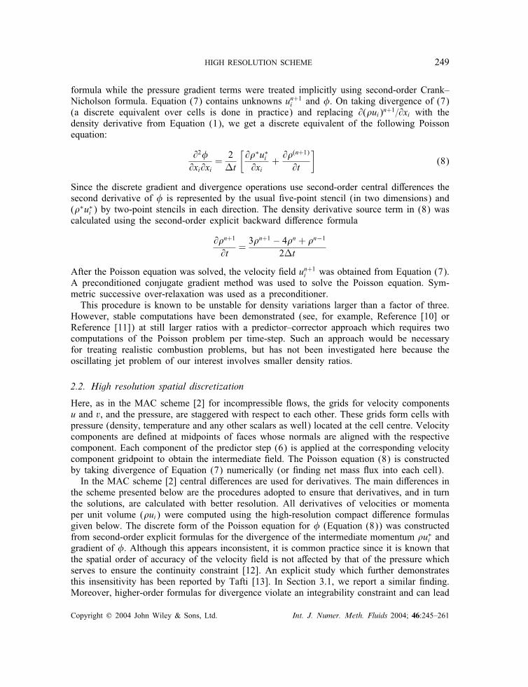
HIGH RESOLUTION SCHEME 251
0 N/20
N/2
k
k~ a
b
c
d
Figure 1. E�ective resolution characteristics of �rst derivative approximations: (a) fourth-order, compact,cell-centred and interpolation −iD∗(k)I(k); (b) fourth-order, compact cell-centred; (c) fourth-order,
compact di�erence; and (d) exact (Fourier).
Second derivatives, for viscous terms, were obtained from the fourth-order formula (�= b=c=0; �=1=10; a=12=10 in formula (2.2.6) of Lele [3])
112f′′i−1 +
1012f′′i +
112f′′i+1 =
fi−1 − 2fi + fi+1�x2
(12)
These derivative and interpolation formulas, (10) and (11), can be written as relations betweenFourier coe�cients: f̂∗(k)= I(k)f̂(k) and f̂′(k)=D∗(k)f̂∗(k)=D∗(k)I(k)f̂(k)= ik̃f̂(k).For exact operations (Fourier), interpolation I(k)=1 and D∗(k)I(k)= ik. Curve a inFigure 1 shows the e�ective resolution resulting from combining interpolation formula (11)with di�erence formula (10) the represented wavenumber range 0¡k¡N=2 when N is thenumber of intervals per period (taken as 2 here). Interpolation reduces the modi�ed wavenum-ber of the cell-centred compact formula (curve b) at the high wavenumber end but remainsslightly better than the standard fourth-order compact formula (curve c). Exact Fourier dif-ferentiation is the straight line k̃= k (curve d). Resolution characteristics of formula (12) forthe second derivative can be found in Reference [3].The implicit formulas (10)–(12) are closed with end conditions. These are boundary equa-
tions which close the implicit formulas and not boundary conditions of the �ow. For interpo-lation the boundary equation used was the implicit third-order formula 3f∗
1=2 +f∗3=2 =f0 + 3f1.
Here, subscript 0 denotes a boundary location. For derivatives, we have used the third-order formula 11f′
1 +f′2 = (−8f∗
1=2 + 16f∗3=2 − 8f1)=h, generally, and the second-order formula
f′1 = (f
∗3=2 −f∗
1=2)=h for derivatives of the cross term uv. For second derivatives, the boundaryequation was the third-order explicit formula f′′
1 = (11f0 − 20f1 + 6f2 + 4f3 − f4)=12h2.The improved resolution o�ered by the compact di�erencing scheme leads to an increased
possibility of aliasing error. Aliasing error becomes most prominent when the shorter lengthscales are marginally resolved and is dependent on aspects of the particular problem. One wayto control aliasing error is to use �ltering [3]. In the present simulations no explicit de-aliasing
Copyright ? 2004 John Wiley & Sons, Ltd. Int. J. Numer. Meth. Fluids 2004; 46:245–261
252 S. CHAKRAVORTY AND J. MATHEW
algorithm has been used, but the discretization does provide for high wavenumber �ltering (seeFigure 1). It is known that discretizations of di�erent forms of the advection terms result indi�erent aliasing errors. In Equation (5), the convective terms are written in the conservativeform @(�ujui)=@xj. Alternate forms are called the non-conservative form �uj@ui=@xj, and theskew-symmetric form 1
2 @�ujui=@xj +12 �uj@ui=@xj +
12 ui@(�uj)=@xj. For incompressible �ow,
aliasing error for the conservative and non-conservative forms are of opposite signs [14]. Sothe skew-symmetric form has been recommended to keep aliasing errors small. As a part ofthe present studies, the conservative, non-conservative and skew-symmetric forms have allbeen tested. Although there are di�erences between the solutions on a given grid, all formsconverged to the ‘correct’ solutions as grids were re�ned.
3. NUMERICAL SOLUTIONS
Three problems are considered to assess di�erent aspects of the proposed high-resolutionmethod. The �rst is the Taylor–Green �ow in two dimensions, which is an incompressible,doubly periodic �ow with a simple closed form solution. The second is the linear instabil-ity stage of incompressible �ow between parallel plates. This is a particularly sensitive testbecause the eigenfunction has a rich structure very close to the plates. To obtain even aqualitatively correct solution requires good resolution. The third case is the variable densityplane jet �ow which motivated this study.
3.1. Taylor–Green problem
The Taylor–Green �ow is a doubly periodic array of two-dimensional vortices of alternatingsense given by
u(x; y; t) =− cos kx sin ky exp(−2k2t=Re)
v(x; y; t) = sin kx cos ky exp(−2k2t=Re)
p(x; y; t) =− 14 (cos 2kx + cos 2ky) exp(−4k2t=Re)
for any wavenumber k. The non-linear terms balance the pressure exactly. So there is only aviscous decay and no growth of harmonics. With the solution at t=0 as the initial condition,solutions at subsequent times were found on a square of side 2. Periodic boundary conditionswere applied in both x and y directions. The present, compact di�erence scheme and thesecond-order, explicit di�erence scheme (MAC) were used.Following Yang et al. [15] who took this �ow to assess the performance of a convolu-
tion algorithm, we simulated at several Reynolds numbers Re=102; 104; 106 and 1010 andwavenumbers k=1; 2 and 5 on the same grid of 32× 32 cells. The time step was �t=0:001.The L∞ error of the u-component for a meaningful subset of these simulations (Re=102; 104
and k=1; 5) are listed in Table I. Also listed are data from Yang et al. [15] of their calcula-tions with a Fourier pseudospectral method. At higher Re the solution changes little and themethods give nearly the same results. As is evident in the tables, the errors in the solutionswith the compact scheme are about two orders of magnitude smaller than those with the
Copyright ? 2004 John Wiley & Sons, Ltd. Int. J. Numer. Meth. Fluids 2004; 46:245–261
HIGH RESOLUTION SCHEME 253
Table I. L∞-error of velocity component u in numerical solutions of the two-dimensionalTaylor–Green �ow. The pseudospectral results are from Yang et al. [15].
k Re t Psuedospectral Second-order explicit Fourth-order compact
1 102 1 1:95E − 10 6:26E − 05 1:21E − 0710 1:52E − 10 5:23E − 04 1:01E − 0620 1:15E − 10 8:57E − 04 1:65E − 0630 8:68E − 11 1:05E − 03 2:03E − 06
1 104 1 7:91E − 13 6:39E − 07 1:23E − 0910 7:59E − 12 6:37E − 06 1:23E − 0820 1:48E − 11 1:27E − 05 2:46E − 0830 2:23E − 11 1:90E − 05 3:68E − 08
5 102 1 6:95E − 08 2:39E − 02 1:21E − 0310 1:40E − 10 3:19E − 03 1:36E − 0420 3:79E − 12 5:32E − 05 1:85E − 06
5 104 1 1:18E − 11 3:85E − 04 1:98E − 0510 1:38E − 06 3:69E − 03 1:89E − 04
100
100
101 102
10-2
10-4
10-6
10-8
103
N
erro
r
slope = -2
slope = -4
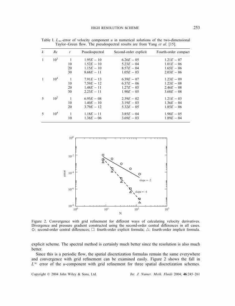
Figure 2. Convergence with grid re�nement for di�erent ways of calculating velocity derivatives.Divergence and pressure gradient constructed using the second-order central di�erences in all cases.◦: second-order central di�erences; : fourth-order explicit formula; �: fourth-order implicit formula.
explicit scheme. The spectral method is certainly much better since the resolution is also muchbetter.Since this is a periodic �ow, the spatial discretization formulas remain the same everywhere
and convergence with grid re�nement can be examined easily. Figure 2 shows the fall inL∞ error of the u-component with grid re�nement for three spatial discretization schemes.
Copyright ? 2004 John Wiley & Sons, Ltd. Int. J. Numer. Meth. Fluids 2004; 46:245–261
254 S. CHAKRAVORTY AND J. MATHEW
Here k=1, Re=100 and the solutions are at t=1. One is with second-order formulas for allderivatives (standard MAC scheme). The second has fourth-order explicit formulas for velocityderivatives of the momentum equations and the third has fourth-order compact di�erences.In all three cases, the divergence of the velocity �eld and the gradient of the pressure wereconstructed using the second order central di�erence formula. Figure 2 shows that the order ofspatial accuracy follows that taken to discretize the velocity derivatives and that the magnitudeof the error is smaller when compact di�erences are used.
3.2. Temporal evolution of small disturbances on Poiseuille �ow
This is a demonstration of both resolving power and long-time accuracy. Standard linearstability analysis of Poiseuille �ow provides eigenfunctions which can be added as a smallperturbation to the base �ow. The evolution of this perturbed �ow obtained using a numericalscheme can be compared against the linear stability solution to assess properties of the nu-merical scheme. We consider both a decaying mode and a growing mode. The decaying modeis a mild test of resolution because the eigenfunction has a simple structure. Resolution errorcan cause a substantial departure for the growing mode because the eigenfunction has a richstructure near channel walls [16]. Even what may be considered reasonable grid clusteringmay not be adequate. Malik et al. [17], who had used Chebychev points, needed far moregrid points compared to Rai and Moin [18] who had used a grid with spacing which grew asa geometric progression. Both had used �nite-di�erence discretizations. So, this is a suitabletest to demonstrate the bene�ts of using a high-resolution scheme.According to linear stability analysis for Poiseuille �ow [19], at a Reynolds number of 7500
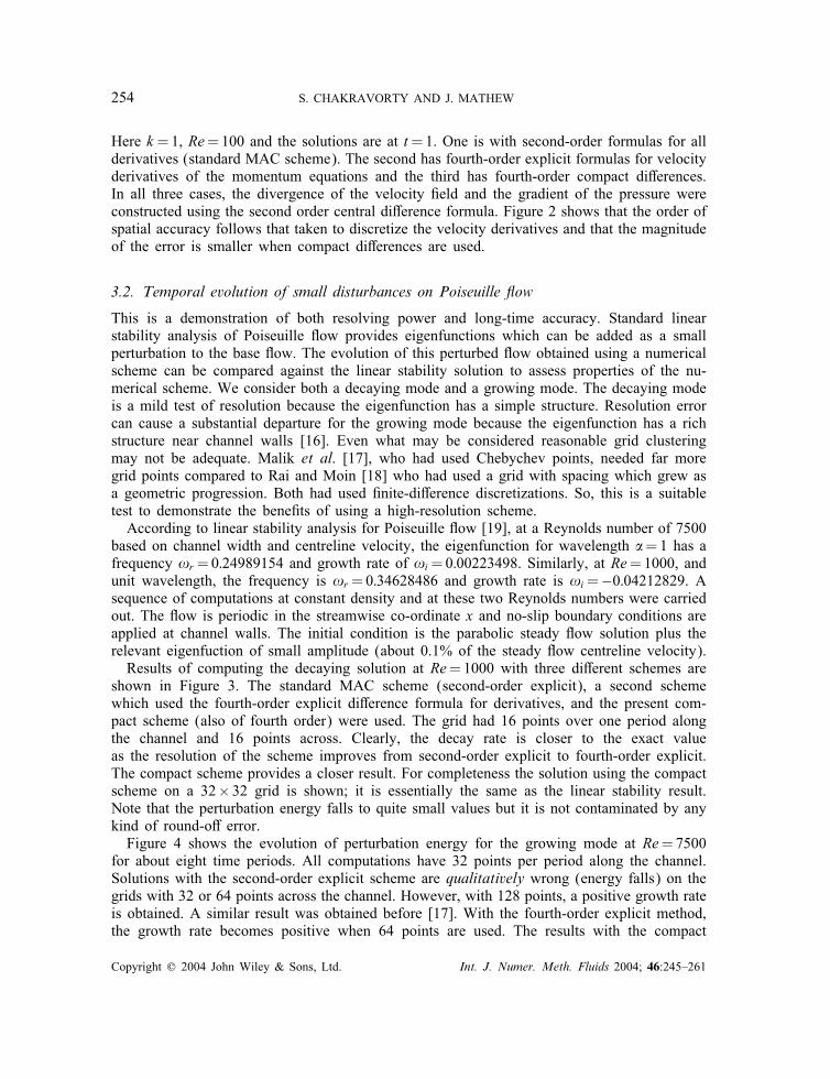
based on channel width and centreline velocity, the eigenfunction for wavelength �=1 has afrequency !r =0:24989154 and growth rate of !i=0:00223498. Similarly, at Re=1000, andunit wavelength, the frequency is !r =0:34628486 and growth rate is !i=−0:04212829. Asequence of computations at constant density and at these two Reynolds numbers were carriedout. The �ow is periodic in the streamwise co-ordinate x and no-slip boundary conditions areapplied at channel walls. The initial condition is the parabolic steady �ow solution plus therelevant eigenfuction of small amplitude (about 0.1% of the steady �ow centreline velocity).Results of computing the decaying solution at Re=1000 with three di�erent schemes are
shown in Figure 3. The standard MAC scheme (second-order explicit), a second schemewhich used the fourth-order explicit di�erence formula for derivatives, and the present com-pact scheme (also of fourth order) were used. The grid had 16 points over one period alongthe channel and 16 points across. Clearly, the decay rate is closer to the exact valueas the resolution of the scheme improves from second-order explicit to fourth-order explicit.The compact scheme provides a closer result. For completeness the solution using the compactscheme on a 32× 32 grid is shown; it is essentially the same as the linear stability result.Note that the perturbation energy falls to quite small values but it is not contaminated by anykind of round-o� error.Figure 4 shows the evolution of perturbation energy for the growing mode at Re=7500
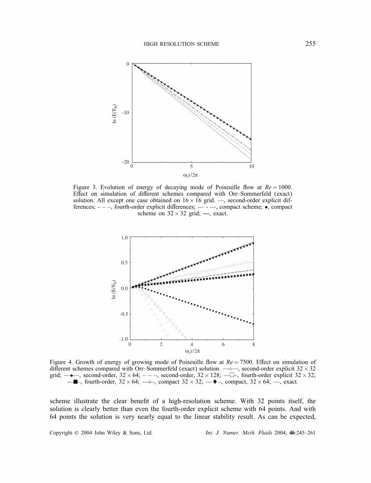
for about eight time periods. All computations have 32 points per period along the channel.Solutions with the second-order explicit scheme are qualitatively wrong (energy falls) on thegrids with 32 or 64 points across the channel. However, with 128 points, a positive growth rateis obtained. A similar result was obtained before [17]. With the fourth-order explicit method,the growth rate becomes positive when 64 points are used. The results with the compact
Copyright ? 2004 John Wiley & Sons, Ltd. Int. J. Numer. Meth. Fluids 2004; 46:245–261
HIGH RESOLUTION SCHEME 255
ωrt/2π
-20
-10
0
ln (
E/E
0)
0 5 10
Figure 3. Evolution of energy of decaying mode of Poiseuille �ow at Re=1000.E�ect on simulation of di�erent schemes compared with Orr–Sommerfeld (exact)solution. All except one case obtained on 16× 16 grid. —, second-order explicit dif-ferences; – – –, fourth-order explicit di�erences; — - —, compact scheme; •, compact
scheme on 32× 32 grid; —, exact.
-1.0
-0.5
0.0
0.5
1.0
0 2 4 6 8ωrt/2π
ln (
E/E
0)
Figure 4. Growth of energy of growing mode of Poiseuille �ow at Re=7500. E�ect on simulation ofdi�erent schemes compared with Orr–Sommerfeld (exact) solution. —◦—, second-order explicit 32× 32grid; —•—, second-order, 32× 64; – – –, second-order, 32× 128; — –, fourth-order explicit 32× 32;
— –, fourth-order, 32× 64; —�–, compact 32× 32; —�–, compact, 32× 64; —, exact.
scheme illustrate the clear bene�t of a high-resolution scheme. With 32 points itself, thesolution is clearly better than even the fourth-order explicit scheme with 64 points. And with64 points the solution is very nearly equal to the linear stability result. As can be expected,
Copyright ? 2004 John Wiley & Sons, Ltd. Int. J. Numer. Meth. Fluids 2004; 46:245–261
256 S. CHAKRAVORTY AND J. MATHEW
the correct result can be obtained at the 32-point resolution itself when using a Chebyshevspectral method, since it has even better resolution characteristics [17].All these solutions were obtained using the skew-symmetric form for the non-linear terms.
The conservative form shows a growth rate which is smaller than the exact rate and convergesfrom below as the grid is re�ned. The non-conservative form converges from above. Sincethe errors in the two are of opposite signs, but not equal in magnitude, the skew-symmetricform gives a closer result for a given grid but oscillates while approaching the exact result.These two examples also emphasize the idea that the bene�ts of a high-resolution scheme
will be realized only when solution structure has �ne scales. In some cases, as in the decayingmode problem, grid re�nement may be su�cient. In others, especially in three-dimensionalcomputations, su�cient grid re�nement may not even be possible. Further, although the higher-order explicit formula also provided some improvement in resolution, the compact scheme ofthe same order provided still further improvement and is, therefore, a more e�cient scheme.
3.3. Unstable, variable-density, plane jet
The high-resolution method presented above was developed to study self-sustained oscillationsof low density jets. It has been observed that oscillations appear in round jets when the ratioof jet to ambient �uid density drops below a critical value. It is observed in helium jetsexhausting into air, heated jets, whether buoyant or not, and also plane jets (see Reference [20]for a plane jet experiment). The phenomenon is due to density variations rather than due tocompressibility e�ects of high speed �ows. Initial computations of plane jets using a standardmethod [9] reproduced self-sustained oscillations, but the �ow �elds seemed incorrect: jet-boundary shear layers rolled up into vortices but, as these vortices traveled downstream, theyslowed down and grew considerably bigger. Wiggles appeared in some regions indicatingloss of resolution. On comparing with solutions obtained with the high-resolution method, itappears that these are O(1) errors which accumulate. So the improvement is important becauseit is not a small quantitative di�erence but is qualitative as well.We consider symmetric solutions (seen in experiments [20]) of the plane jet �ow which are
determined by the velocity and density pro�les at the in�ow plane. The streamwise velocitycomponent and density were
u(x=0; y)=12
[1+ tanh
(2�!(y − y0)
)](13)
�(x=0; y)=12
[1′ + tanh
(2�!(y − y0)
)](14)
The jet velocity at the centreline is Uj and velocity far from the jet when there is a co-�owis Ua. In Equation (13) =(Uj −Ua)=(Uj +Ua) is a measure of the intensity of shearing, �!is the shear layer vorticity thickness and the centre of the shear layer is at y=y0. Similarly,in Equation (14), the density pro�le is characterized by the parameter ′=(R − 1)=(R + 1)where R=�j=�a is the jet to ambient �uid density ratio. No initial or in�ow perturbations wereimposed. Oscillations appeared spontaneously when the density ratio R¡0:9, approximately,as in experiments. For a uniform density �ow (R=1), perturbations at the in�ow plane willcause the jet shear layers to roll up into vortices, but this instability disappears—vortices areconvected out—when in�ow perturbations are turned o�.
Copyright ? 2004 John Wiley & Sons, Ltd. Int. J. Numer. Meth. Fluids 2004; 46:245–261
HIGH RESOLUTION SCHEME 257
A slip boundary condition was prescribed along the lateral planes to mimic freestreamconditions. Prescribing out�ow boundary conditions is always a sensitive issue in a spatiallydeveloping, unsteady �ow. The boundary condition should be consistent with the physicalprocesses of the �ow. Since the out�ow plane is a truncation of the jet, some error due tothis truncation can be expected. The aim in such a situation would be to ensure that �owstructures leaving the computational domain should do so with minimal distortion and withoutre�ections travelling to every part of the computational domain. Here, the advective boundarycondition,
@�ui@t
+Ue@�ui@x
=0
was used along the out�ow plane as in Reference [21]. Additionally, a correction was appliedalong the out�ow plane to ensure overall mass balance [11]. Also, the location of the out�owboundary was progressively taken farther away and the frequency of oscillation was monitored.With velocity di�erence across the jet shear layer as the velocity scale and vorticity thick-
ness at in�ow as the length scale (�!=1), simulations were conducted at Reynolds numberRe=570 and Prandtl number Pr=0:7. The Reynolds number based on initial jet width y0 = 8is then Rey0 = 4560.The computational domain was a rectangle 120 units long in the streamwise direction and 40
units in the transverse direction on one side of the jet centreline. A uniform grid of 480× 320points gives a good solution with the present high-resolution scheme. On a coarse grid of240× 160 points, the lack of resolution shows up as wiggles. With the standard, second-orderexplicit scheme, even with a �ner grid of 720× 480 points the solution is not well-resolvedeverywhere.On the coarse grid, computation time was roughly the same for both schemes. Most of the
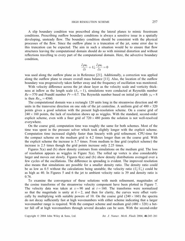
time was spent in the pressure solver which took slightly longer with the explicit scheme.Computation time increased slightly faster than linearly with grid re�nement. CPU-time forthe compact scheme on the medium grid is 4.2 times longer than on the coarse grid. Withthe explicit scheme the increase is 5.7 times. From medium to �ne grid (explicit scheme) theincrease is 2.5 times though the grid points increase only 2.25 times.Figures 5(a) and (b) show density contours from simulations on the medium grid. The loss
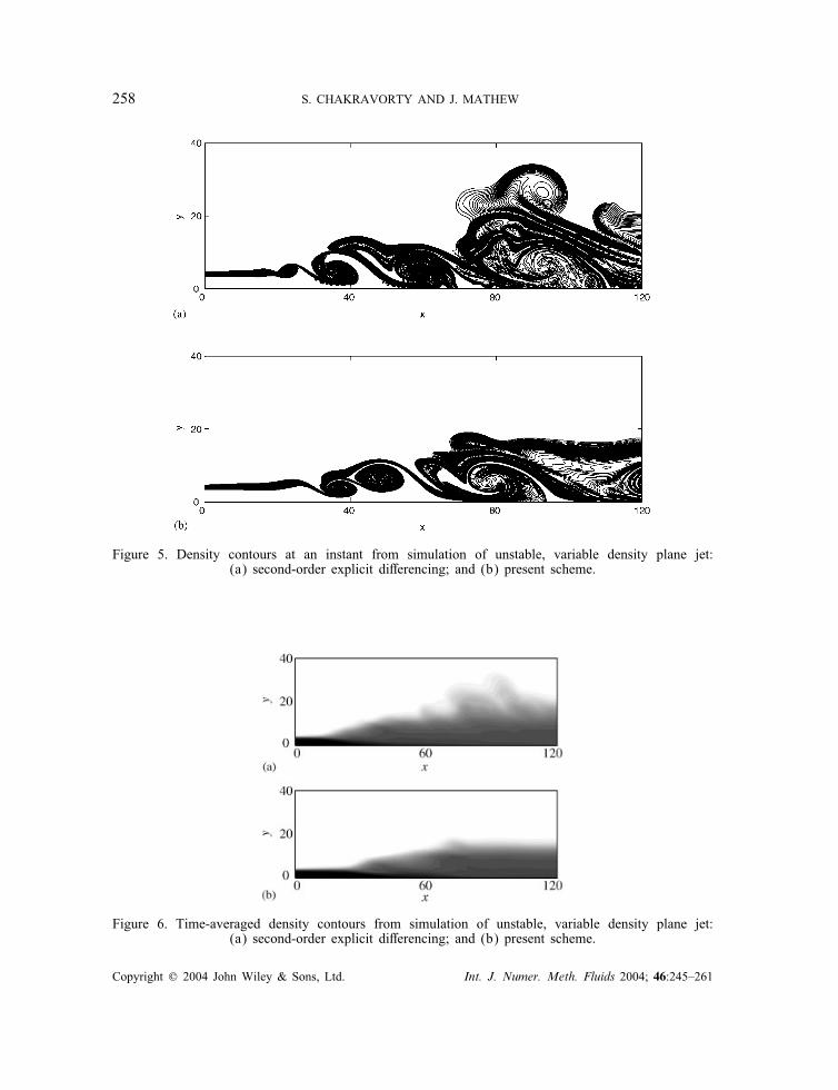
of resolution appears as wiggles in Figure 5(a). The rolled up vortex is also considerablylarger and moves out slowly. Figures 6(a) and (b) show density distributions averaged over afew cycles of the oscillations. The di�erence in spreading is evident. The improved resolutionalso means that simulations are possible for a smaller density ratio. The density ratio couldbe as low as 0.5 without the calculations being unstable; the velocity ratio (Uj=Ua) could beas high as 40. In Figures 5 and 6 the jet to ambient velocity ratio is 39 and density ratio is0.76.To examine the convergence of these solutions with mesh re�nement, magnitudes of
the cosine transforms of the streamwise velocity component have been plotted in Figure 7.The velocity data was taken at x=90 and at t=160. The transforms were normalizedso that the magnitude is unity at k=2, and then for clarity, the curves were o�set verti-cally by multiplying with suitable powers of 10. On the coarse grid (240× 160) the spectrado not decay su�ciently fast at high wavenumbers with either scheme indicating that a largerwavenumber range is required. With the compact scheme and medium grid (480× 320) a bet-ter fall o� at high wavenumbers through several decades can be seen. With the second-order
Copyright ? 2004 John Wiley & Sons, Ltd. Int. J. Numer. Meth. Fluids 2004; 46:245–261
258 S. CHAKRAVORTY AND J. MATHEW
Figure 5. Density contours at an instant from simulation of unstable, variable density plane jet:(a) second-order explicit di�erencing; and (b) present scheme.
Figure 6. Time-averaged density contours from simulation of unstable, variable density plane jet:(a) second-order explicit di�erencing; and (b) present scheme.
Copyright ? 2004 John Wiley & Sons, Ltd. Int. J. Numer. Meth. Fluids 2004; 46:245–261
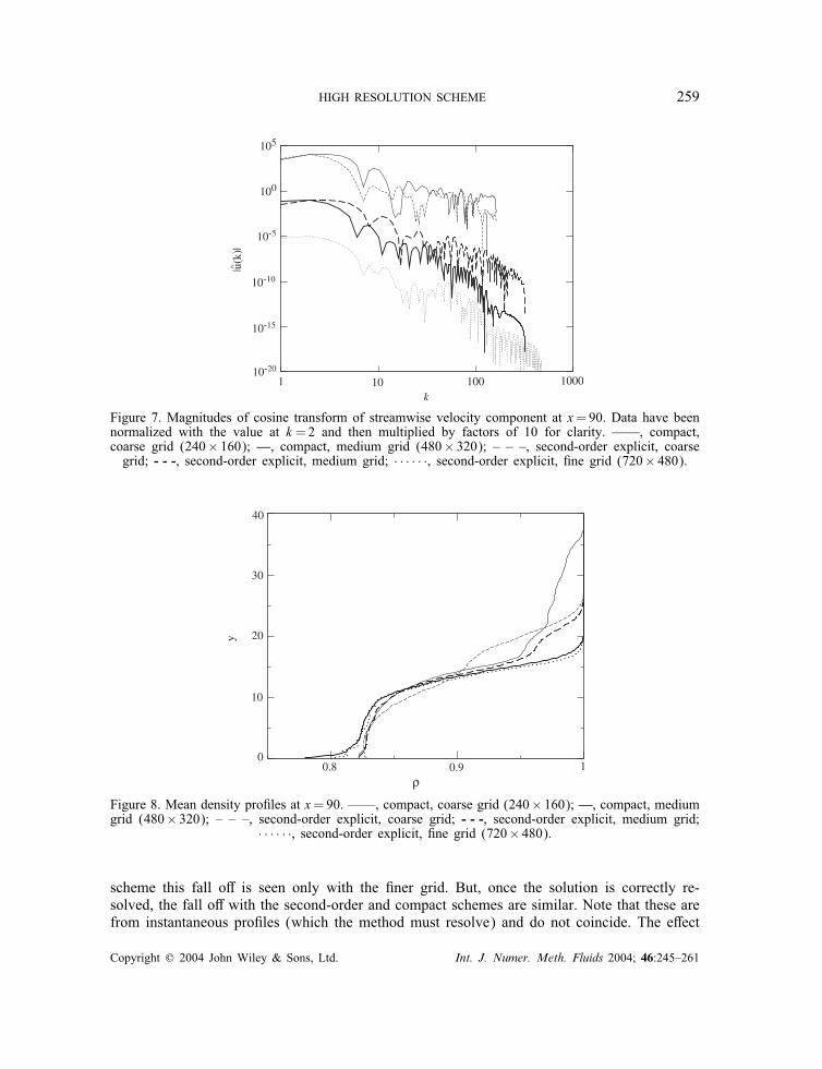
HIGH RESOLUTION SCHEME 259
1 10 100 1000k
10-10
100
105
10-5
10-15
10-20
|u(k
)|∧
Figure 7. Magnitudes of cosine transform of streamwise velocity component at x=90. Data have beennormalized with the value at k =2 and then multiplied by factors of 10 for clarity. ——, compact,coarse grid (240× 160); —, compact, medium grid (480× 320); – – –, second-order explicit, coarsegrid; - - -, second-order explicit, medium grid; · · · · · ·, second-order explicit, �ne grid (720× 480).
0.8 0.9 10
10
20
30
40
y
ρ
Figure 8. Mean density pro�les at x=90. ——, compact, coarse grid (240× 160); —, compact, mediumgrid (480× 320); – – –, second-order explicit, coarse grid; - - -, second-order explicit, medium grid;
· · · · · ·, second-order explicit, �ne grid (720× 480).
scheme this fall o� is seen only with the �ner grid. But, once the solution is correctly re-solved, the fall o� with the second-order and compact schemes are similar. Note that these arefrom instantaneous pro�les (which the method must resolve) and do not coincide. The e�ect
Copyright ? 2004 John Wiley & Sons, Ltd. Int. J. Numer. Meth. Fluids 2004; 46:245–261
260 S. CHAKRAVORTY AND J. MATHEW
of under-resolution is not a mere clipping of a correct spectrum, but a wrong spectral distri-bution. In physical space this shows up as wiggles. The convergence of the mean �ow can beseen in Figure 8. Mean density pro�les at x=90 taken from the same �ve computations havebeen plotted. Coarse grid solutions are not very di�erent from the �ner grid solutions overa part of the interface between light and heavy �uid. The di�erences are largely towards theouter edge of the jet (as can be inferred from Figures 5 and 6). These excursions at the outeredge disappear on the medium grid with the compact scheme and on the �ne grid solutionwith the explicit scheme.
4. CONCLUSIONS
In this paper, some observations made in the course of developing an algorithm for lowMach number �ow were presented. Spatial derivatives were obtained using implicit di�erenceformulas which have better resolving power allowing a larger range of scales to be computedaccurately. The test of channel �ow linear instability clearly illustrates the bene�cial e�ects ofthe high-resolution scheme. For the unstable, low density jet, the compact scheme was ableto capture sharp density gradients without spurious oscillations. Solutions remained smoothand stable computations over a wider range of sensitive parameters such as density ratio andco-�ow velocity ratio were obtained.
REFERENCES
1. Majda M, Sethian J. The derivation and numerical solution of the equations for zero Mach number combustion.Combustion Science and Technology 1985; 42:185–205.
2. Harlow FH, Welch JE. Numerical calculation of three dependent viscous incompressible �ow of �uid with freesurface. Physics of Fluids 1965; 8:2182–2189.
3. Lele SK. Compact �nite di�erence schemes with spectral-like resolution. Journal of Computational Physics1992; 103:16–42.
4. Sabanca M, Brenner G, Alemdaroglu N. Improvements to compressible Euler methods for low-Mach number�ows. International Journal for Numerical Methods in Fluids 2000; 34:167–185.
5. Morinishi Y, Lund TS, Vasilyev OV, Moin P. Fully conservative higher order �nite di�erence schemes forincompressible �ow. Journal of Computational Physics 1998; 143:90–124.
6. Nicoud F. Conservative high-order �nite-di�erence schemes for low-Mach number �ows. Journal ofComputational Physics 2000; 158:71–97.
7. Bell JB, Marcus DL. A second-order projection method for variable density �ows. Journal of ComputationalPhysics 1992; 101:334–348.
8. Almgren AS, Bell JB, Colella P, Howell LH, Welcome ML. A conservative adaptive projection method for thevariable density incompressible Navier–Stokes equations. Journal of Computational Physics 1998; 142:1–46.
9. McMurtry PA, Jou WH, Riley JJ, Metcalfe RW. Direct numerical simulation of a reacting mixing layer withchemical heat release. AIAA Journal 1986; 24(6):962–970.
10. Najm HN, Wycko� PS, Knio OM. A semi-implicit numerical scheme for reacting �ow. Journal ofComputational Physics 1998; 143:381–402.
11. Boersma BJ. Direct simulation of a jet di�usion �ame. Annual Research Briefs 1998; Center for TurbulenceResearch, Stanford University, Stanford, 1998; 47–56.
12. Perot JB. An analysis of the fractional step method. Journal of Computational Physics 1993; 108:51–58.13. Tafti D. Comparison of some upwind-biased high-order formulations with a second-order central-di�erence
scheme for time integrations of the incompressible Navier–Stokes equations. Computer & Fluids 1996; 25:647–665.
14. Kravchenko AG, Moin P. On the e�ect of numerical errors in large eddy simulations of turbulent �ows. Journalof Computational Physics 1997; 131:310–322.
15. Yang SY, Zhou YC, Wei GW. Comparison of the discrete singular convolution algorithm and the Fourierpseudospectral method for solving partial di�erential equations. Computer Physics Communication 2002;143:113–135.
Copyright ? 2004 John Wiley & Sons, Ltd. Int. J. Numer. Meth. Fluids 2004; 46:245–261
HIGH RESOLUTION SCHEME 261
16. Das A, Mathew J. Direct numerical simulation of turbulent spots. Computer & Fluids 2001; 30:533–541.17. Malik MR, Zang TA, Hussaini MY. A spectral collocation method for the Navier–Stokes equation. Journal of
Computational Physics 1985; 61:64–88.18. Rai MM, Moin P. Direct simulations of turbulent �ow using �nite-di�erence schemes. Journal of Computational
Physics 1991; 96:15–53.19. Orszag SA. Accurate solution of the Orr–Sommerfeld stability equation. Journal of Fluid Mechanics 1971;
50:689–703.20. Yu M, Monkewitz PA. Oscillations in the near �eld of a heated two-dimensional jet. Journal of Fluid Mechanics
1993; 255:323–347.21. Lowery PS, Reynolds WC. Numerical simulation of a spatially-developing, forced, plane mixing layer. Report
No. TF-26. Department of Mechanical Engineering, Stanford University, Stanford, 1986.
Copyright ? 2004 John Wiley & Sons, Ltd. Int. J. Numer. Meth. Fluids 2004; 46:245–261