a handcrafted normalized-convolution network for texture...
TRANSCRIPT
A Handcrafted Normalized-Convolution Network for Texture Classification
Vu-Lam Nguyen
Ngoc-Son Vu
Philippe-Henri Gosselin
ETIS/Universite Paris Seine, Universite Cergy-Pontoise, ENSEA, CNRS
95000-Cergy, France
Tel.:+33 01 30 73 66 10
Fax: +33 01 30 73 66 27
Abstract
In this paper, we propose a Handcrafted Normalized-
Convolution Network (NmzNet) for efficient texture classifi-
cation. NmzNet is implemented by a three-layer normalized
convolution network, which computes successive normal-
ized convolution with a predefined filter bank (Gabor filter
bank) and modulus non-linearities. Coefficients from differ-
ent layers are aggregated by Fisher Vector aggregation to
form the final discriminative features. The results of exper-
imental evaluation on three texture datasets UIUC, KTH-
TIPS-2a, and KTH-TIPS-2b indicate that our proposed ap-
proach achieves the good classification rate compared with
other handcrafted methods. The results additionally indi-
cate that only a marginal difference exists between the best
classification rate of recent frontiers CNN and that of the
proposed method on the experimented datasets.
1. Introduction
Texture provides important clues for identifying materi-
als and objects, especially when their shapes are not avail-
able. A wide range of applications such as industrial in-
spection, image retrieval, medical imaging, remote sensing,
object and facial recognition can be developed depend upon
analyzing the textures of their surfaces. Hence, texture anal-
ysis includes segmentation, shape extraction, synthesis, and
classification is an active field.
There are variety texture analysis approaches have been
proposed. They can be ranged from a simple to sophisti-
cated computation strategy methods. Simple yet efficient
feature extraction approaches can be a long list. They can
be: 1) local binary pattern (LBP) method [32] and its vari-
ants; 2) the representation based on co-occurrence matrix
[16]; 3) the filter-based approaches such as works in [2, 30];
4) the wavelet transform method as works in [28, 20, 4]; 5)
the texton dictionary-based [22, 43, 44]; 6) the use of bidi-
rectional features [8, 9]; and so on. In addition, many so-
phisticated computation strategy methods have been intro-
duced to improve the feature robustness and performance.
Scattering Network (ScatNet) [41], and Convolutional neu-
ral network (CNNs) with Fisher vector CNN (FV+CNN)
delegation [6] belong to this category.
Among those approaches, the LBP-family can be con-
sidered as a popular feature method which extracts well lo-
cal micro-structure information from images. Ojala et al.
[31] first introduced the LBP method in 1996, then a multi-
resolution version [32] in 2002. After that, several exten-
sions on LBP have been conducted. In 2007, Tan et al.
extended LBP to three-valued codes to become the local
ternary pattern (LTP) [42]. Liao et al. proposed dominant
LBP (DLBP) [23] which combines the most frequently oc-
curred patterns with the Gabor filter responses for features.
Later Guo et al. introduced completed LBP (CLBP) [12],
which merges three components the sign (CLBP S), mag-
nitude (CLBP M), and center pixel intensity (CLBP C) to-
gether to form features. This enhances discriminative power
compared to the original version. Variance in LBP (LBPV)
[13] is utilized to encode local contrast information without
requiring a quantization process, and rotation invariance is
implemented by estimating principal orientations and align-
ing LBP histograms. By constructing a cascading spatial
pyramid of LBP, Qian et al. [37] introduced pyramid trans-
formed LBP (PLBP), the robustness of PLBP was compared
with those of other LBP variants in this works. Further, Liu
et al. suggested extended LBP [26] by a combination of
pixel intensities and local differences. In this way, the pixel
intensity part is divided into a central pixel’s component
and neighbor’s component. Likewise, the local difference
consists of two components: radial differences and an an-
11238
gular difference. At the end, those four were combined to
form features. In addition, Zhao et al. in [51] presented lo-
cal binary pattern histograms of Fourier features (LBP-HF)
which implement rotation invariance by computing discrete
Fourier transforms of LBP histograms. In [11], moreover,
Guo et al. presented a three-layered learning framework in
which LTP and CLBP were used as raw features to train and
select the discriminative features.
Contrary to the micro-structure descriptors of LBP fam-
ily, several broader range feature methods have been devel-
oped. Bovik et al. applied the Gabor filters to compute
the average filter responses for features [2]. Mallat pro-
posed the multi-resolution wavelet decomposition method
[29], which generates coefficients from the high-low (HL),
low-high (LH), and low-low (LL) channels for subsequent
classification tasks. Porter et al. [34] removed the high-
high (HH) wavelet channels and combined the LH and HL
wavelet channels to obtain rotation invariance wavelet fea-
tures. Haley et al. [15] calculated isotropic rotation invari-
ance features from Gabor filter responses. More recent,
scattering transform is considered as a high-performance
approach based on cascading wavelet transform layers [41]
compared to previous wavelet-based methods.
The paper is organized as follows: we start with a review
of the normalized convolution in Section 2.1, Fisher vector
aggregation presented in Section 2.2, followed by details of
the derivation of the proposed approach (Section 2.3). Sec-
tion 2.4 presents the proposed method. In Section 3, we
verify the our approach with experiments on popular tex-
ture datasets and comparisons with various state-of-the-art
texture classification techniques. Section 4 provides con-
cluding remarks and possible extensions of the proposed
method.
2. Proposed Handcrafted Network
In this section, we propose a handcrafted Normalized-
Convolution Network with its derivation described in 2.1,
2.1, and 2.2 for efficient texture classification.
2.1. Normalized Convolution
Normalized convolution was introduced by Knutsson
and Westin in [19]. It is a method for performing gen-
eral convolution operations on data of signal/certainty type.
More specifically, it takes into account the uncertainties in
signal values and allows spatial localization of possibly un-
limited analysis functions. The conceptual basis for the
method is the signal/certainty philosophy, i.e. separating
the values of a signal from the certainty of the measure-
ments. The separation of both data and operator into a sig-
nal part and a certainty part. Missing data is simply handled
by setting the certainty to zero. In the case of uncertain
data, an estimate of the certainty must accompany the data.
Localization or windowing of operators is done using an
applicability function, the operator equivalent to certainty,
not by changing the actual operator coefficients. Spatially
or temporally limited operators are handled by setting the
applicability function to zero outside the window.
Formally, Knutsson et al. define normalized convolution
in form of standard convolution as follows,
U(ξ) =∑
a(x)B(x)⊙ c(ξ − x)T (ξ − x) (1)
where
ξ is the global spatial coordinate.
x is the local spatial coordinate.
T (ξ) is a tensor corresponding to the input signal.
c(ξ) is a function which represents the certainty of T (ξ).B(x) is a tensor corresponding to the operator filter basis.
a(x) is the operator equivalent to certainty, a function which
represents the applicability of B(x).⊙ denotes multi-linear operations (in standard convolu-
tion this operation is scalar multiplication). When the ba-
sic operation is understood explicitly indicating the depen-
dence on the global spatial coordinates ξ, the local spatial
coordinate x plays no role. Then, the expression (1) can be
written as
U = {aB⊙cT} (2)
where the “hat“ over the multilinear operation symbol acts
as a marker of the operation involved in the convolution
(it is useful when more than one operation symbol appears
within the brackets).
Knutsson et al. also draw another definition of normal-
ized convolution by the means of general convolution oper-
ations on data of signal/certainty type. Normalized convo-
lution of aB and cT can be defined and denoted by:
UN = {aB⊙cT}N = N−1D (3)
where: D = {aB⊙cT}N = aB ⊙B∗ .c
The star, ∗, is the complex conjugate operator.
The concept of normalized convolution has a theory be-
hind, the least squares problem.
To see this, express a given neighbourhood, t, in a set of
basis functions given by a matrix B and the coefficients u.
(standard matrix and vector notation are used.)
t′ = Bu (4)
It is proved that for a given set of basis functions, B , the
least square error, ‖t′ − t‖, is minimized by choosing u to
be:
u =[BTB
]−1BT t (5)
With the introduction of a diagonal matrix, W, a weighted
least square problem can be solved by
Wt′ =WBu (6)
1239
Then the minimum of ‖W (t′ − t)‖ is obtained by choosing
coefficients u to be:
u =[(WB)
TWB
]−1
(WB)TWt (7)
which can be rewritten and split into two parts,N−1 andD.
u =[BTW 2B
]−1
︸ ︷︷ ︸N
BTW 2t︸ ︷︷ ︸D
(8)
It can be shown that N and D are identical to the corre-
sponding quantities used in normalized convolution, equa-
tion (3). In normalized convolution, the diagonal weight
matrix is, for a neighbourhood centered on ξ0, given by:
W 2ii (ξ0) = a (xi) c (ξ0 − xi) (9)
Therefore, normalized convolution can be considered as a
method used to obtain a local weighted least square er-
ror representation of the input signal. The input signal is
described in terms of the basis function set, B, while the
weights are adaptive and given by the data certainties and
the operator applicability.
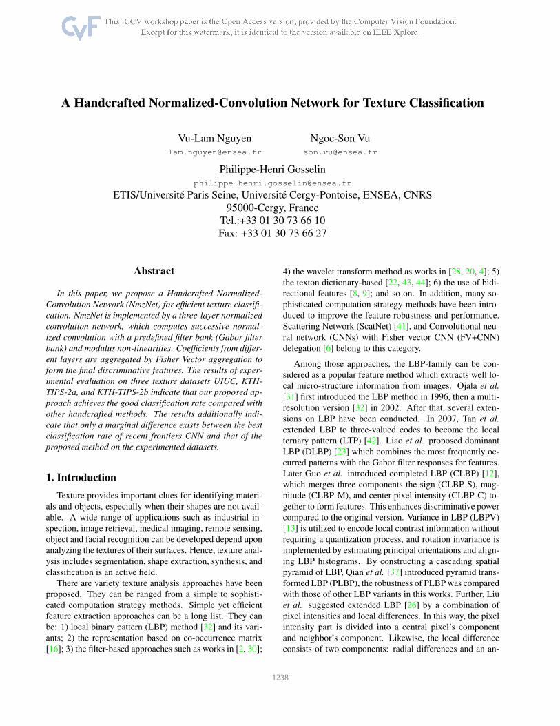
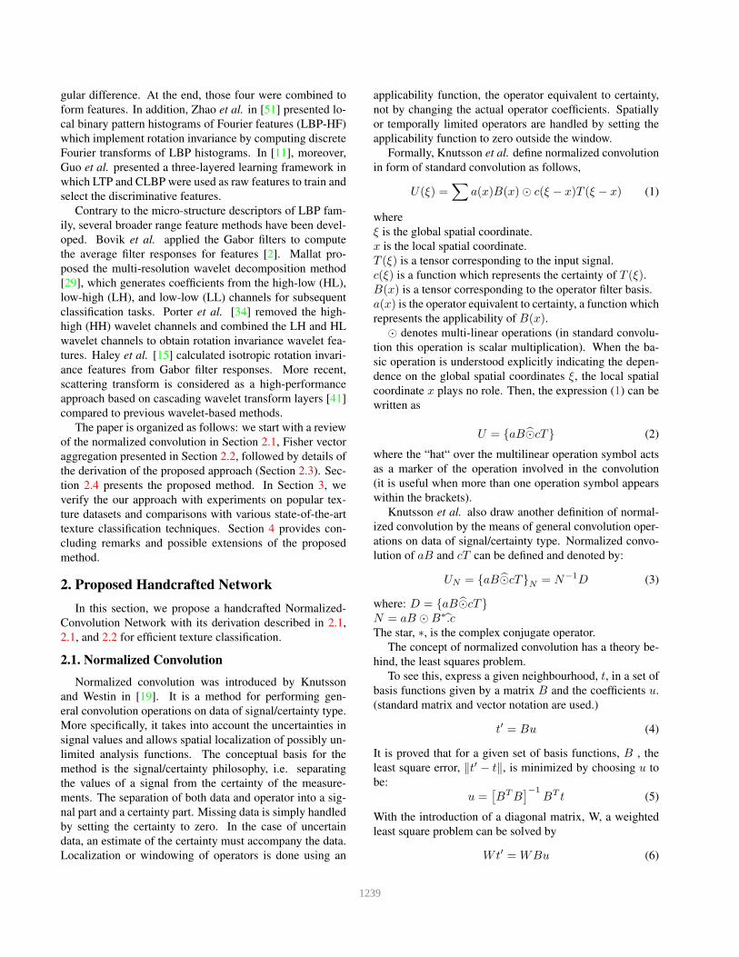
One of the most striking applications of normalized con-
volution might be the interpolation of Lena image (Figure
2) using applicability function illustrated in Figure 1.
015
0.2
0.4
1510
0.6
0.8
10
1
55
0 0
Figure 1. An applicability function.
2.2. Fisher Vectors
This section describes the Fisher Vector (FV) of [33] .
The FV is an image representation obtained by pooling lo-
cal image features. It is frequently used as a global image
descriptor in visual classification. Given an input image I ,
the Fisher Vector (FV) formulation of [33] starts by extract-
ing local descriptors X = {xt, t = 1 · · ·T}, they can be
densely and at multiple scales. It is assumed that X can be
modeled by a probability density function uλ, with λ is the
set of parameters of u as well as the estimation of those.
Then, X can be described by the gradient vector as
GλX =
1
T▽λ log uλ(X) (10)
Since Fisher information matrix (Fλ) of probability den-
sity function (uλ) is symmetric and positive, it has the
50
100
150
200
250
300
350
400
450
500
50
100
150
200
250
300
350
400
450
500
50
100
150
200
250
300
350
400
450
500
50
100
150
200
250
300
350
400
450
500
Figure 2. Top left: The famous Lena-image, top right the image
has been degraded to a grey-level test image only containing 20%
of the original information. Bottom left: Interpolation using stan-
dard convolution with a normalized smoothing filter (see Figure
1). Bottom right: Interpolation using normalized convolution with
the same filter as applicability function.
Cholesky decomposition Fλ = L′
λLλ. Therefore, the
Fisher kernel can be written as a dot-product between nor-
malized gradient vectors Γλ, with ΓXλ = LλG
Xλ , and ΓX
λ is
referred to as the Fisher vector of X .
The probability density function uλ is chosen to
be a Gaussian Mixture Model (GMM): uλ (x) =∑Ki=1
wiui (x), and λ = {wi, µi,Σi, i = 1 · · ·K} where
wi, µi, and Σi are mixture weight, mean vector and covari-
ance matrix of Gaussian ui respectively. Covariance matri-
ces are assumed to be diagonal, and σ2i denotes the variance
vector. The local descriptors xt are assumed to be generated
independently from uλ, and therefore:
GXλ =
1
T
T∑
t=1
▽λ log uλ (xt) . (11)
Soft assignment (γt) of descriptor xt to Gaussian i is com-
puted as
γt (i) =wiui (xt)∑K
j=1wjuj (xt)
. (12)
Let ΓXµ,i be the gradient vector computed on the mean µi,
and ΓXσ,i be the gradient vector computed on the standard
deviation σi of Gaussian i, then derivative of those will lead
to formulations for computing the first and second order
1240
statistics of the local descriptors.
ΓXµ,i =
1
T√wi
T∑
t=1
γt (i)
(xt − µi
σi
). (13)
ΓXσ,i =
1
T√2wi
T∑
t=1
γt (i)
[(xt − µi)
2
σ2i
− 1
]. (14)
The final Fisher vector is the concatenation of the ΓXσ,i and
ΓXσ,i vectors for i = 1...K, with the dimensionality is 2KD,
D is the dimension of a descriptor xt.
2.3. Scattering Network
Scattering Network (ScatNet) [27] is a handcrafted deep
convolution network, in which cascade of wavelet trans-
form and modulus non-linearities operators are consecu-
tively computed to form the network layers. As illustrated
in Figure 3, each |Wm| outputs invariant scattering coeffi-
cients Smx and the next layer of covariant wavelet modu-
lus coefficients Um+1x, which is further transformed by the
subsequent wavelet-modulus operators.
|W1 |
S0x
U1x |W2 |
S1x
U2x |W3 |
S2x
...
Figure 3. Scattering network formed by wavelet-modulus cascad-
ing
The average Smx carries only the low frequencies
of Umx while the high frequencies are captured by
roto-translation convolutions with wavelets. |Wm| trans-
forms Umx into the average Smx and a new layer
Um+1x of wavelet amplitude coefficients: |Wm|(Umx) =(Smx, Um+1x). Repetitively computing this wavelet mod-
ulus transform would generate multiple layers of scattering
invariant coefficients. For m = 0 U0x = x, in case the
network has three layers, the scattering feature vector (Sx)
would be a concatenation of three Six coefficients such that
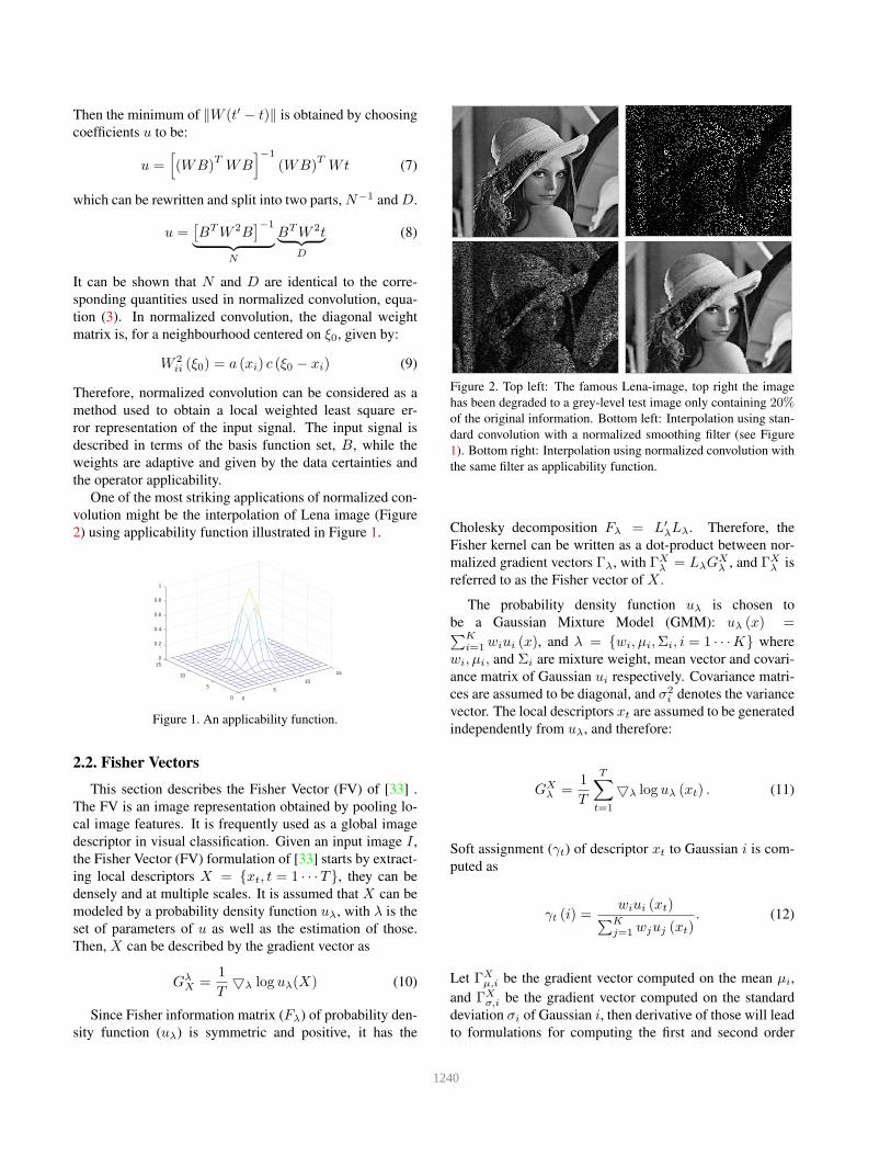
Sx = (S0x, S1x, S2x). A filter bank of low-pass and high-
pass filters for implementing Morlet wavelet (Wm operator)
is illustrated in Figure 4.
2.4. NormalizedConvolution Network
This section introduces a handcrafted network which in-
herits ScatNet [41] for texture classification. In this novel
handcrafted network, so called Normalized-Convolution
Network (NmzNet), we propose two important changes to
the ScatNet (section 2.3) to enhance its robustness.
i) We modify the wavelet modulus operator, the funda-
mental operator of ScatNet, by a substitution of the normal-
Figure 4. Complex Morlet wavelets with Gaussian kernel (top
left corner), different scales (along rows) and orientations (along
columns). The real and imaginary parts are shown on the left and
on the right, respectively.
ized convolution presented in section 2.1 for the standard
convolution used in ScatNet as flows
The operator of the first network layer:
W1x =(x⊛ φJ , {|x⊛ ψθ,j |}θ,j
)= (S0x, U1x) (15)
where ⊛ is the normalized convolution operator.
|.| is the modulus operator.
j = 1...J is the scaling parameter.
φJ and ψθ,j are respectively the low and high pass filter ker-
nels with J scales and θ angles. These kernels used as ap-
plicability functions for the normalized convolution in our
proposed method.
The wavelet-modulus operator for layers m ≥ 2 com-
puted on Um−1x the same way as the one on the first layer.
However, there is a normalized convolution computed along
the angle parameters taken into account.
ii) The average pooling of ScatNet replaced by the Fish
Vector feature aggregation in the NmzNet.
Given an image I , local descriptors {d1, ..., dn} are ex-
tracted from three different layers of NmzNet. These fea-
tures are then soft-quantized using a Gaussian Mixture
Model (GMM). Subsequently, the dimensionality is re-
duced by PCA before concatenating their first and second
order statistics to form the final Fisher Vector features. We
have discovered that our proposed method improves clas-
sification accuracy on the tested texture benchmarks (see
Section 3).
3. Experimental Results
This section evaluates the proposed method for classi-
fying texture data. First, parameter settings and datasets
are presented. Second, we evaluate the results and com-
pare with the state-of-the-art. Finally, we analyze the pro-
posed method and its complexity. In our experiments, we
used source code of ScatNet, VLFeat library shared by Mal-
lat’s team [41], and Vedaldi et al. [45, 46] respectively to
generate texture classification results on three benchmarks:
UIUC, KTH-TIPS-2a, and KTH-TIPS-2b.
1241
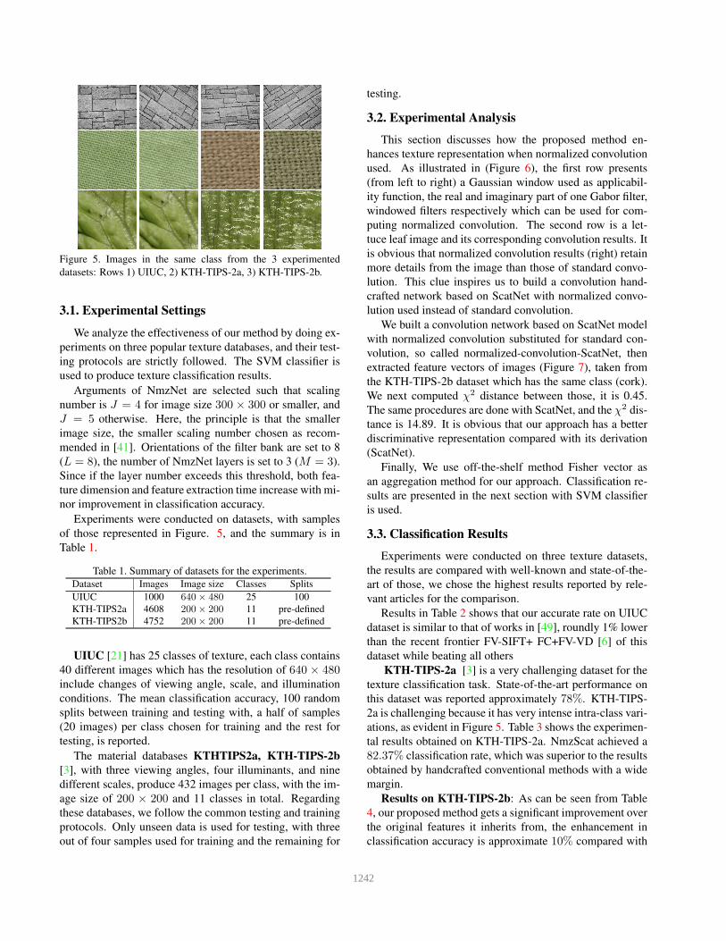
Figure 5. Images in the same class from the 3 experimented
datasets: Rows 1) UIUC, 2) KTH-TIPS-2a, 3) KTH-TIPS-2b.
3.1. Experimental Settings
We analyze the effectiveness of our method by doing ex-
periments on three popular texture databases, and their test-
ing protocols are strictly followed. The SVM classifier is
used to produce texture classification results.
Arguments of NmzNet are selected such that scaling
number is J = 4 for image size 300 × 300 or smaller, and
J = 5 otherwise. Here, the principle is that the smaller
image size, the smaller scaling number chosen as recom-
mended in [41]. Orientations of the filter bank are set to 8
(L = 8), the number of NmzNet layers is set to 3 (M = 3).
Since if the layer number exceeds this threshold, both fea-
ture dimension and feature extraction time increase with mi-
nor improvement in classification accuracy.
Experiments were conducted on datasets, with samples
of those represented in Figure. 5, and the summary is in
Table 1.
Table 1. Summary of datasets for the experiments.
Dataset Images Image size Classes Splits
UIUC 1000 640× 480 25 100
KTH-TIPS2a 4608 200× 200 11 pre-defined
KTH-TIPS2b 4752 200× 200 11 pre-defined
UIUC [21] has 25 classes of texture, each class contains
40 different images which has the resolution of 640 × 480include changes of viewing angle, scale, and illumination
conditions. The mean classification accuracy, 100 random
splits between training and testing with, a half of samples
(20 images) per class chosen for training and the rest for
testing, is reported.
The material databases KTHTIPS2a, KTH-TIPS-2b
[3], with three viewing angles, four illuminants, and nine
different scales, produce 432 images per class, with the im-
age size of 200 × 200 and 11 classes in total. Regarding
these databases, we follow the common testing and training
protocols. Only unseen data is used for testing, with three
out of four samples used for training and the remaining for
testing.
3.2. Experimental Analysis
This section discusses how the proposed method en-
hances texture representation when normalized convolution
used. As illustrated in (Figure 6), the first row presents
(from left to right) a Gaussian window used as applicabil-
ity function, the real and imaginary part of one Gabor filter,
windowed filters respectively which can be used for com-
puting normalized convolution. The second row is a let-
tuce leaf image and its corresponding convolution results. It
is obvious that normalized convolution results (right) retain
more details from the image than those of standard convo-
lution. This clue inspires us to build a convolution hand-
crafted network based on ScatNet with normalized convo-
lution used instead of standard convolution.
We built a convolution network based on ScatNet model
with normalized convolution substituted for standard con-
volution, so called normalized-convolution-ScatNet, then
extracted feature vectors of images (Figure 7), taken from
the KTH-TIPS-2b dataset which has the same class (cork).
We next computed χ2 distance between those, it is 0.45.
The same procedures are done with ScatNet, and the χ2 dis-
tance is 14.89. It is obvious that our approach has a better
discriminative representation compared with its derivation
(ScatNet).
Finally, We use off-the-shelf method Fisher vector as
an aggregation method for our approach. Classification re-
sults are presented in the next section with SVM classifier
is used.
3.3. Classification Results
Experiments were conducted on three texture datasets,
the results are compared with well-known and state-of-the-
art of those, we chose the highest results reported by rele-
vant articles for the comparison.
Results in Table 2 shows that our accurate rate on UIUC
dataset is similar to that of works in [49], roundly 1% lower
than the recent frontier FV-SIFT+ FC+FV-VD [6] of this
dataset while beating all others
KTH-TIPS-2a [3] is a very challenging dataset for the
texture classification task. State-of-the-art performance on
this dataset was reported approximately 78%. KTH-TIPS-
2a is challenging because it has very intense intra-class vari-
ations, as evident in Figure 5. Table 3 shows the experimen-
tal results obtained on KTH-TIPS-2a. NmzScat achieved a
82.37% classification rate, which was superior to the results
obtained by handcrafted conventional methods with a wide
margin.
Results on KTH-TIPS-2b: As can be seen from Table
4, our proposed method gets a significant improvement over
the original features it inherits from, the enhancement in
classification accuracy is approximate 10% compared with
1242
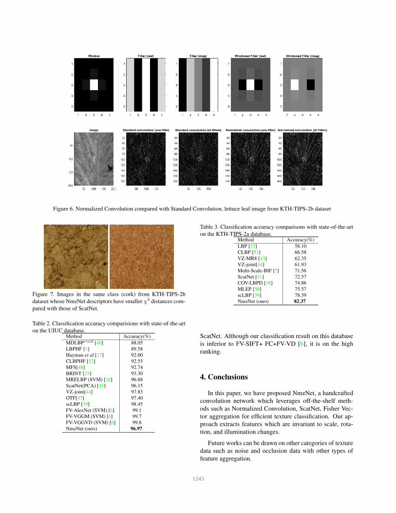
Figure 6. Normalized Convolution compared with Standard Convolution, lettuce leaf image from KTH-TIPS-2b dataset
Figure 7. Images in the same class (cork) from KTH-TIPS-2b
dataset whose NmzNet descriptors have smaller χ2 distances com-
pared with those of ScatNet.
Table 2. Classification accuracy comparisions with state-of-the-art
on the UIUC database.Method Accuracy(%)
MDLBPriu2 [40] 88.05
LBPHF [1] 89.58
Hayman et al.[17] 92.00
CLBPHF [52] 92.55
MFS[48] 92.74
BRINT [25] 93.30
MRELBP (SVM) [24] 96.88
ScatNet(PCA) [41] 96.15
VZ-joint[44] 97.83
OTF[47] 97.40
scLBP [39] 98.45
FV-AlexNet (SVM) [6] 99.1
FV-VGGM (SVM) [6] 99.7
FV-VGGVD (SVM) [6] 99.8
NmzNet (ours) 96.97
Table 3. Classification accuracy comparisons with state-of-the-art
on the KTH-TIPS-2a database.Method Accuracy(%)
LBP [32] 58.10
CLBP [53] 66.58
VZ-MR8 [43] 62.35
VZ-joint[44] 61.93
Multi-Scale-BIF [7] 71.56
ScatNet [41] 72.57
COV-LBPD [18] 74.86
MLEP [50] 75.57
scLBP [39] 78.39
NmzNet (ours) 82.37
ScatNet. Although our classification result on this database
is inferior to FV-SIFT+ FC+FV-VD [6], it is on the high
ranking.
4. Conclusions
In this paper, we have proposed NmzNet, a handcrafted
convolution network which leverages off-the-shelf meth-
ods such as Normalized Convolution, ScatNet, Fisher Vec-
tor aggregation for efficient texture classification. Our ap-
proach extracts features which are invariant to scale, rota-
tion, and illumination changes.
Future works can be drawn on other categories of texture
data such as noise and occlusion data with other types of
feature aggregation.
1243
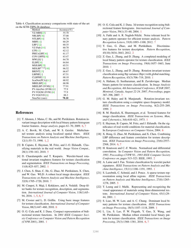
Table 4. Classification accuracy comparisons with state-of-the-art
on the KTH-TIPS-2b database.Method Accuracy(%)
VZ-MR8[43] 55.70
NRLBP[38] 57.00
NTLBP[10] 58.78
MBP[14] 60.29
LBP [32] 60.35
VZ-Path [44] 60.70
LTP[42] 62.12
PRICoLBP[36] 61.17
COV-LBPD[18] 63.47
MWLD[5] 64.70
ELBP[26] 64.84
MSJLBP[35] 65.51
MDLBPriu2[40] 66.52
BRINT[25] 66.67
LBPHF[1] 67.51
CLBPHF[52] 68.10
ScatNet(PCA)[41] 68.92
MRELBP[24] 68.98
MRELBP (SVM)[24] 77.91
FV-AlexNet (SVM) [6] 77.9
FV-VGGM (SVM) [6] 77.9
FV-VGGVD [6] 88.2
NmzNet (ours) 78.10
References
[1] T. Ahonen, J. Matas, C. He, and M. Pietikainen. Rotation in-
variant image description with local binary pattern histogram
fourier features. Image analysis, pages 61–70, 2009. 6, 7
[2] A. C. Bovik, M. Clark, and W. S. Geisler. Multichan-
nel texture analysis using localized spatial filters. IEEE
Transactions on Pattern Analysis and Machine Intelligence,
12(1):55–73, 1990. 1, 2
[3] B. Caputo, E. Hayman, M. Fritz, and J.-O. Eklundh. Clas-
sifying materials in the real world. Image Vision Comput.,
28(1):150–163, 2010. 5
[4] D. Charalampidis and T. Kasparis. Wavelet-based rota-
tional invariant roughness features for texture classification
and segmentation. IEEE Transactions on Image Processing,
11(8):825–837, 2002. 1
[5] J. Chen, S. Shan, C. He, G. Zhao, M. Pietikainen, X. Chen,
and W. Gao. WLD: A robust local image descriptor. IEEE
Transactions on Pattern Analysis and Machine Intelligence,
32(9):1705–1720, 2010. 7
[6] M. Cimpoi, S. Maji, I. Kokkinos, and A. Vedaldi. Deep fil-
ter banks for texture recognition, description, and segmenta-
tion. International Journal of Computer Vision, 118(1):65–
94, 2016. 1, 5, 6, 7
[7] M. Crosier and L. D. Griffin. Using basic image features
for texture classification. International Journal of Computer
Vision, 88(3):447–460, 2010. 6
[8] O. G. Cula and K. J. Dana. Compact representation of bidi-
rectional texture functions. In 2001 IEEE Computer Soci-
ety Conference on Computer Vision and Pattern Recognition
(CVPR 2001), 2001. 1
[9] O. G. Cula and K. J. Dana. 3d texture recognition using bidi-
rectional feature histograms. International Journal of Com-
puter Vision, 59(1):33–60, 2004. 1
[10] A. Fathi and A. R. Naghsh-Nilchi. Noise tolerant local bi-
nary pattern operator for efficient texture analysis. Pattern
Recognition Letters, 33(9):1093–1100, 2012. 7
[11] Y. Guo, G. Zhao, and M. PietikaInen. Discrimina-
tive features for texture description. Pattern Recognition,
45(10):3834–3843, 2012. 2
[12] Z. Guo, L. Zhang, and D. Zhang. A completed modeling of
local binary pattern operator for texture classification. IEEE
Transactions on Image Processing, 19(6):1657–1663, June
2010. 1
[13] Z. Guo, L. Zhang, and D. Zhang. Rotation invariant texture
classification using lbp variance (lbpv) with global matching.
Pattern Recognition, 43(3):706–719, 2010. 1
[14] A. Hafiane, G. Seetharaman, and B. Zavidovique. Median
binary pattern for textures classification. In Image Analysis
and Recognition, 4th International Conference, ICIAR 2007,
Montreal, Canada, August 22-24, 2007, Proceedings, pages
387–398, 2007. 7
[15] G. M. Haley and B. Manjunath. Rotation-invariant tex-
ture classification using a complete space-frequency model.
IEEE Transactions on Image Processing, 8(2):255–269,
1999. 2
[16] R. M. Haralick, K. Shanmugam, et al. Textural features for
image classification. IEEE Transactions on Systems, Man,
and Cybernetics, 3(6):610–621, 1973. 1
[17] E. Hayman, B. Caputo, M. Fritz, and J. Eklundh. On the sig-
nificance of real-world conditions for material classification.
In European Conference on Computer Vision, 2004. 6
[18] X. Hong, G. Zhao, M. Pietikainen, and X. Chen. Combining
LBP difference and feature correlation for texture descrip-
tion. IEEE Transactions on Image Processing, 23(6):2557–
2568, 2014. 6, 7
[19] H. Knutsson and C.-F. Westin. Normalized and differential
convolution. In Computer Vision and Pattern Recognition,
1993. Proceedings CVPR’93., 1993 IEEE Computer Society
Conference on, pages 515–523. IEEE, 1993. 2
[20] A. Laine and J. Fan. Texture classification by wavelet packet
signatures. IEEE Transactions on Pattern Analysis and Ma-
chine Intelligence, 15(11):1186–1191, 1993. 1
[21] S. Lazebnik, C. Schmid, and J. Ponce. A sparse texture rep-
resentation using local affine regions. IEEE Transactions
on Pattern Analysis and Machine Intelligence, 27(8):1265–
1278, 2005. 5
[22] T. Leung and J. Malik. Representing and recognizing the
visual appearance of materials using three-dimensional tex-
tons. International Journal of Computer Vision, 43(1):29–
44, 2001. 1
[23] S. Liao, M. W. Law, and A. C. Chung. Dominant local bi-
nary patterns for texture classification. IEEE Transactions
on Image Processing, 18(5):1107–1118, 2009. 1
[24] L. Liu, S. Lao, P. W. Fieguth, Y. Guo, X. Wang, and
M. Pietikainen. Median robust extended local binary pat-
tern for texture classification. IEEE Transactions on Image
Processing, 25(3):1368–1381, 2016. 6, 7
1244
[25] L. Liu, Y. Long, P. W. Fieguth, S. Lao, and G. Zhao. Brint:
binary rotation invariant and noise tolerant texture classifica-
tion. IEEE Transactions on Image Processing, 23(7):3071–
3084, 2014. 6, 7
[26] L. Liu, L. Zhao, Y. Long, G. Kuang, and P. Fieguth. Ex-
tended local binary patterns for texture classification. Image
and Vision Computing, 30(2):86–99, 2012. 1, 7
[27] S. Mallat. Group Invariant Scattering. Communications on
Pure and Applied Mathematics, 65(10):1331–1398, 2012. 4
[28] S. G. Mallat. A theory for multiresolution signal decom-
position: the wavelet representation. IEEE Transactions on
Pattern Analysis and Machine Intelligence, 11(7):674–693,
1989. 1
[29] S. G. Mallat. A theory for multiresolution signal decom-
position: the wavelet representation. IEEE Transactions on
Pattern Analysis and Machine Intelligence, 11(7):674–693,
1989. 2
[30] B. S. Manjunath and W.-Y. Ma. Texture features for brows-
ing and retrieval of image data. IEEE Transactions on
Pattern Analysis and Machine Intelligence, 18(8):837–842,
1996. 1
[31] T. Ojala, M. Pietikainen, and D. Harwood. A comparative
study of texture measures with classification based on fea-
tured distributions. Pattern Recognition, 29(1):51–59, 1996.
1
[32] T. Ojala, M. Pietikainen, and T. Maenpaa. Multiresolution
gray-scale and rotation invariant texture classification with
local binary patterns. IEEE Transactions on Pattern Analysis
and Machine Intelligence, 2002. 1, 6, 7
[33] F. Perronnin and C. Dance. Fisher kernels on visual vocab-
ularies for image categorization. In Computer Vision and
Pattern Recognition, 2007. CVPR’07. IEEE Conference on,
pages 1–8. IEEE, 2007. 3
[34] R. Porter and N. Canagarajah. Robust rotation-invariant
texture classification: wavelet, gabor filter and gmrf based
schemes. IEE Proceedings-Vision, Image and Signal Pro-
cessing, 144(3):180–188, 1997. 2
[35] X. Qi, Y. Qiao, C. Li, and J. Guo. Multi-scale joint encoding
of local binary patterns for texture and material classifica-
tion. In British Machine Vision Conference, BMVC 2013,
Bristol, UK, September 9-13, 2013, 2013. 7
[36] X. Qi, R. Xiao, C.-G. Li, Y. Qiao, J. Guo, and X. Tang. Pair-
wise rotation invariant co-occurrence local binary pattern.
Pattern Analysis and Machine Intelligence, IEEE Transac-
tions on, 36(11):2199–2213, 2014. 7
[37] X. Qian, X.-S. Hua, P. Chen, and L. Ke. Plbp: An effective
local binary patterns texture descriptor with pyramid repre-
sentation. Pattern Recognition, 44(10):2502–2515, 2011. 1
[38] J. Ren, X. Jiang, and J. Yuan. Noise-resistant local bi-
nary pattern with an embedded error-correction mechanism.
IEEE Transactions on Image Processing, 22(10):4049–4060,
2013. 7
[39] J. Ryu, S. Hong, and H. S. Yang. Sorted consecutive local
binary pattern for texture classification. IEEE Transactions
on Image Processing, 24(7):2254–2265, 2015. 6
[40] G. Schaefer and N. P. Doshi. Multi-dimensional local binary
pattern descriptors for improved texture analysis. In Pattern
Recognition (ICPR), 2012 21st International Conference on,
pages 2500–2503. IEEE, 2012. 6, 7
[41] L. Sifre and S. Mallat. Rotation, scaling and deformation in-
variant scattering for texture discrimination. In 2013 IEEE
Conference on Computer Vision and Pattern Recognition,
pages 1233–1240, 2013. 1, 2, 4, 5, 6, 7
[42] X. Tan and B. Triggs. Enhanced local texture feature sets
for face recognition under difficult lighting conditions. In
Analysis and Modeling of Faces and Gestures, pages 168–
182. Springer, 2007. 1, 7
[43] M. Varma and A. Zisserman. A statistical approach to texture
classification from single images. Int. Journal of Computer
Vision, 62(1-2):61–81, 2005. 1, 6, 7
[44] M. Varma and A. Zisserman. A statistical approach to ma-
terial classification using image patch exemplars. IEEE
Transactions on Pattern Analysis and Machine Intelligence,
31(11):2032–2047, 2009. 1, 6, 7
[45] A. Vedaldi and B. Fulkerson. VLFeat: An open and portable
library of computer vision algorithms. http://www.
vlfeat.org/, 2010. 4
[46] A. Vedaldi and K. Lenc. Matconvnet – convolutional neural
networks for matlab. In Proceeding of the ACM Int. Conf. on
Multimedia, 2015. 4
[47] Y. Xu, S. Huang, H. Ji, and C. Fermuller. Combining power-
ful local and global statistics for texture description. In 2009
IEEE Computer Society Conference on Computer Vision and
Pattern Recognition (CVPR 2009), 20-25 June 2009, Miami,
Florida, USA, pages 573–580, 2009. 6
[48] Y. Xu, H. Ji, and C. Fermuller. Viewpoint invariant texture
description using fractal analysis. International Journal of
Computer Vision, 83(1):85–100, 2009. 6
[49] Y. Xu, X. Yang, H. Ling, and H. Ji. A new texture descriptor
using multifractal analysis in multi-orientation wavelet pyra-
mid. In CVPR, pages 161–168, 2010. 5
[50] J. Zhang, J. Liang, and H. Zhao. Local energy pattern for
texture classification using self-adaptive quantization thresh-
olds. IEEE transactions on image processing, 22(1):31–42,
2013. 6
[51] G. Zhao, T. Ahonen, J. Matas, and M. Pietikainen. Rotation-
invariant image and video description with local binary pat-
tern features. IEEE Transactions on Image Processing,
21(4):1465–1477, 2012. 2
[52] G. Zhao, T. Ahonen, J. Matas, and M. Pietikainen. Rotation-
invariant image and video description with local binary pat-
tern features. IEEE Transactions on Image Processing,
21(4):1465–1477, 2012. 6, 7
[53] Y. Zhao, D.-S. Huang, and W. Jia. Completed local
binary count for rotation invariant texture classification.
IEEE Transactions on Image Processing, 21(10):4492–4497,
2012. 6
1245