a general methodology for the analysis of experiments with repeated measurement of categorical data

A General Methodology for the Analysis of Experiments with Repeated Measurement ofCategorical DataAuthor(s): Gary G. Koch, J. Richard Landis, Jean L. Freeman, Daniel H. Freeman, Jr. andRobert G. LehnenSource: Biometrics, Vol. 33, No. 1 (Mar., 1977), pp. 133-158Published by: International Biometric SocietyStable URL: http://www.jstor.org/stable/2529309 .

Accessed: 27/06/2014 06:12

Your use of the JSTOR archive indicates your acceptance of the Terms & Conditions of Use, available at .http://www.jstor.org/page/info/about/policies/terms.jsp

.JSTOR is a not-for-profit service that helps scholars, researchers, and students discover, use, and build upon a wide range ofcontent in a trusted digital archive. We use information technology and tools to increase productivity and facilitate new formsof scholarship. For more information about JSTOR, please contact [email protected].

.

International Biometric Society is collaborating with JSTOR to digitize, preserve and extend access toBiometrics.

http://www.jstor.org

This content downloaded from 130.60.206.42 on Fri, 27 Jun 2014 06:12:04 AMAll use subject to JSTOR Terms and Conditions

http://www.jstor.org/action/showPublisher?publisherCode=ibs

http://www.jstor.org/stable/2529309?origin=JSTOR-pdf

http://www.jstor.org/page/info/about/policies/terms.jsp


BIOMETRICS 33, 133-158 March 1977

A General Methodology for the Analysis of Experiments with Repeated Measurement of Categorical Data

GARY G. KOCH

department of Biostatistics, University of North Carolina, Chapel Hill, North Carolina 27514 U.S.A.

J. RICHARD LANDIS

I)epartment of Biostatistics, University of Michigan, Ann Arbor, Michigan 48109 U.S.A.

JEAN L. FREEMAN and DANIEL IT. FREEMAN, JR.

School of Medicine, Yale University, New Haven, Connecticut 06510 U.S.A.

ROBERT G. LEHNEN

I)epartmrnenit of Political Science, University of IJoiusion, Houstoii, Texas 77004 U.S.A.

Suimm ary

This paper is concerned with the analysis of multivariate categorical data which are obtained from repeated measurement experiments. An expository discussion of pertinent hypotheses for such situations is given, and appropriate test statistics are developed through the application of weighted least squares methods. Special consideration is given to computational problems associated with the manipulation of large tables including the treatment of empty cells. Three applications of the methodology are provided.

1. Introduction

Koch and Reinfurt [1971] discussed the statistical analysis of multivariate categorical data from "mixed model" and "split plot" experiments. Such designs are classical prototypes of what are often called "repeated measurement designs," because they involve the collection of inherently multivariate data from the same subject for the same conceptual response variable under two or more experimental and/or observational conditions. The nature and range of application of these designs in the life and social sciences is illustrated by the following examples:

1. Bacteria samples are obtained from throats of each of n subjects with a particular infection. From each sample, three cultures are randomly assigned to three drugs. Each subject provides information about the effectiveness of the three drugs. For further discussion, see Section 3.1.

2. Three drugs are compared for relief of persistent symptoms of a chronic disease, e.g., asthma. Because of variation among patients, a two-period change-over design is used. This design involves the random assignment of paired sequences of drugs to patients who are then observed for two time periods with the first drug in the sequence being used in the first period and the other in the second period. For further discussion. see Section 3.2.

Key Words: Repeated measurement experiments; Multivariate categorical data; Weighted least squares.

133



134 BIOMETRICS, MARCH 1977

3. A new drug and a standard drug are compared for patients with both mild and severe diagnoses of a disease, e.g., skin infection, mental depression, etc. Patients in each diagnosis group are randomly assigned to two drugs and their condition is evaluated as normal or abnormal at the end of one week, two weeks, and four weeks of continuous treatment. For further discussion, see Section 3.3. Analogous examples pertaining to behavioral development of children are given in Landis and Koch [1977c].

4. The agreement among two or more observers is evaluated with respect to the diagnosis of a disease like multiple sclerosis from patient record information, e.g., physical examinations, laboratory tests, family history, etc. Each subject is classified by each observer into a diagnostic category, e.g., certain multiple sclerosis; probable multiple sclerosis; possible multiple sclerosis; and doubtful, unlikely, or definitely not multiple sclerosis. For further discussion, see Landis [1975] and Landis and Koch [1975a, 1975b, 1977a, 1977b].

5. Multivariate paired comparison experiments are undertaken to obtain information on such phenomena as

a. the desired family size of women in an age and marital status group regarding their preferences for elements within pairs, e.g., two children vs. four children, one child vs. five children, no children vs. three children, etc.

b. the quality of soft drinks regarding preferences of subjects evaluating two pairs from four soft drinks according to two criteria-taste and fizziness.

For further discussion, see Davidson and Bradley [1969], Koch, Abernathy and Imrey [1975], Fienberg and Larntz [1976], and Imrey, Johnson and Koch [1976].

6. A longitudinal panel survey is conducted to compare demographic groups regarding their political preferences for three presidential candidates at three time points prior to an election. Each respondent is interviewed at each time point. For further discussion, see Lehnen and Koch [1974a] and Bishop, Fienberg and Holland [1975, Chapter 7].

7. A political survey is conducted to compare the level of trust demographic groups have for three political institutions-the Presidency, the Supreme Court and the Senate. Attitudes toward the three institutions are obtained from each respondent. For further discussion, see Lehnen and Koch [1974b].

8. A political survey is conducted to compare preferences of demographic groups for seven tax expenditure policy alternatives. Each respondent is asked to rank the seven tax alternatives from "most desirable" to "least desirable." For further discussion, see Koch, Freeman, and Lehnen [1976].

For each of the preceding examples, subjects selected from s subpopulations are exposed to d different measurement conditions, e.g., drugs, time periods, stimuli like attitudes toward political candidates, governmental institutions, tax expenditure policies, etc., and are classified for each in terms of a response variable with L levels. More complex applications often involve incomplete research designs for which different subsets of the d conditions (or set of stimuli) are measured on different subjects. Consideration of this broader topic is given in Koch, Imrey and Reinfurt [1972], Lehnen and Koch [1974a], Hocking and Oxspring [1974], and Chen and Fienberg [1974].

Questions of substantive interest for experiments (or surveys) with repeated measurements like (1)-(8) are as follows:

i. Are there any differences among the s sub-populations regarding the average distribution of the responses to the d conditions?



ANALYSIS OF MULTIVARIATE CATEGORICAL DATA 135

ii. Are there any differences among the d conditions regarding the average distribution across the s sub-populations?

iii. Are there any differences among the s sub-populations for differences among the distribution of responses to the d conditions?

These questions are analogous to hypotheses of "no whole-plot effects," "no split-plot effects," and "no whole-plot x split-plot interaction" in split-plot experiments as described in Anderson and Bancroft [1952], Federer [1955] or Steel and Torrie [1960]. Here, however, such hypotheses must be formulated in terms of an underlying (s X r) contingency table where r = Ld represents the number of possible multivariate response profiles. This is discussed in Section 2 where the set of univariate marginal distributions for the d measurement conditions within the s sub-populations contain information for dealing with the questions (i)-(iii). Test statistics for such hypotheses and the estimators of parameters for underlying linear regression models are obtained through weighted least squares computations by methods described in Grizzle, Starmer and Koch [1969] (hereafter GSK) as reviewed in Appendix 1.

The resulting methodology represents a categorical data analogue to more well-known counterparts for quantitative data like multivariate analysis of variance as described by Cole and Grizzle [1966] and Morrison [1967] in the parametric case, and multivariate rank analysis as described by Koch [1969, 1970] in the non-parametric case. Three examples which illustrate the scope of such analyses are discussed in Section 3.

2. Methodology

For repeated measurement experiments, each subject is observed under each of d different conditions, e.g., treatments, policy questions, time points, etc., and the corresponding responses are each classified in terms of L categories. Thus, there are r = Ld possible multivariate response profiles. In accordance with the general framework in Appendix 1, these response profiles will be indexed by a vector subscript j = (il , i id) where j, -

1, 2, * , L for g = 1, 2, , d. As a result, rij = irii2. id represents the joint probability of response profile j for randomly selected subjects from the ith sub-population. If there are no differences among the sub-populations, then the {7rij I satisfy the hypothesis,

Hs: rij= = = 7i'j for all j; (2.1)

similarly, if there are no differences among the d conditions, the 17rij I satisfy the hypothesis of total symmetry

He: 7j = riz(j) for all j and i = 1, 2, * , s, (2.2)

where z(j) is any permutation of j. These hypotheses, with no interaction formulations (discussed in Bhapkar and Koch [1968a, 1968b]), can be tested by the general GSK methodology outlined in Appendix 1. However, these statistical tests are of limited interest since the quantities, which provide the most obvious indication of the relative effects associated with the respective measurement conditions and sub-populations, are the first order marginal probabilities

i = 1, 2, ... ,s 1kiok 7ri i 2, * d for g = 1, 2, , /d. (2.3)

j with jg=k k = 1, 2, , L

Here, 4'ik represents the probability of the kth response category for the gth condition in




the ith sub-population. If there are no differences among the sub-populations (i.e., (2.1)), then the { } satisfy the hypothesis,

THSJ 4)1,k = 02,k = =Dsuk for g= 1,2, I, (2.4)

while if there are no differences among the conditions (i.e., 2.2) then the {i } satisfy the hypothesis of first order m7naigyiulal symmnietry (homiogeneity)

H('fO l = = kf idk for (2.5) k =1, 2,

L ., 25

Thus, it logically follows that

H8,,, false -e Hs8 false (2.6)

HC, false-> H(6 false (2.7)

which means that H,, (or H0J) must be rejected whenever H;S,,I (or HfcAl) is rejected. Alternatively, situations where HsAI (or Hc0Al) is true, regardless of whether H8s (or Hc0) is true, would be interpreted as involving no gross (macro) differences among the sub- populations (conditions). Thus, the hypotheses HSM and HOAI are of interest with respect to investigating the effects of sub-populations and conditions on the response distribution under study.

\lMoreover, HS,, (or HcmOM) have greater logical relevance for this purpose than Hsj (or Hc,). This view can be justified by noting that the additional constraints on the wrj , associated with H, j (or H0 j) but not Hs11 (or H c1), involve relatively complicated equations which do not have a straightforward interpretation. Also, these constraints are partially confounded with those pertaining to the patterns of association, i.e., lack of independence, among the responses to the respective measurement conditions, since the hypothesis,

d

H.,1 : ri i = i2J "',id for all j and i = 1, 2. , s, (2.8)

of joint independence in conjunction with HASA3 (or HIc,) necessarily imply H8,, (or Hci). In repeated measurement experiments, such association is present to the extent that underlying subjects effects cause measurements under two different conditions on the same subject to be more similar than corresponding measurements on different subjects. This type of dependence among responses may be further complicated by factors pertaining to the adjacency of measurements in time and space, e.g., in some longitudinal studies, measurements from adjacent time points are often more related to one another than those for distant time points. Since such association can be present without having any bearing on the interpretation of sub-population and condition effects, it becomes appropriate to remove the corresponding constraints from Hs , and Hc J; but this, of course, yields HSA, and HcM . For most practical purposes, consideration can often be restricted to HSAI and Hc0 in repeated measurement experiments (or surveys). Statistical tests directed at Hs A, and HcM tend to have better asymptotic convergence properties (regarding the valid application of Central Limit Theory (CLT) arguments) in moderately large samples than those directed at Hs , and Hc , since they involve fewer constraint equations, i.e., degrees of freedom (d.f.). This aspect of the analysis of repeated measurement experiments is further discussed in Appendix 2.



ANALYSIS OF MULTIVARJATE CATEGORICAL DATA 137

The hypothesis of no interaction between conditions and sub-populations can be formulated for the {?Io j} in terms of the model

i= 1,2, s HAM : Oio = MU/ + ti*k + r*L, for q = 1, 2, , ci, (2.9)

k = 1, 2, , .

where A/k is an overall mean associated with the kth response category, i*k is an effect due to the ith sub-population, and r*1, is an effect due to the gth condition and where it is usually understood that the {u, } Ji*k } and {T*gk I satisfy the following types of constraints

L I I

Ly= 1, Sti, 0=, STUM 0, /;=1 I =1 1=_ (2.10)

E li* = />3 T*gk,= 0O

as a consequence of (A.2) and certain parameter identifiability considerations, i.e., removal of logical redundancies among parameters. If the model (2.9) is appropriate, then the hypothesis HSM1I in (2.4) implies

HS,, IAMI t1*k = 02*k = = = 0 for k = 1, 2, *, L, (2.11)

and the hypothesis HCMI in (2.5) implies

HCI1AAI: T*1k = T*2k =' '*dk 0 for lc = 1, 2, , L. (2.12)

Other hypotheses can be formulated to account for any inherent structure associated with the s sub-populations or the d conditions, e.g., trends or separate roles of two or more underlying factors. In some cases, it may be more appropriate to work with multiplicative no interaction models in which the additivity relationships like (2.9) pertain to the { log Oigk

(see Bhapkar and Koch [1968a, 1968b]). An example of this is given in Section 3.3. These considerations can be extended further if the response categories lc = 1, 2, , L

are ordinally scaled with progressively larger intensities. In this event, the effects of the respective sub-populations and measurement conditions can be compared in one or more of the following cumulative marginal probability functions:

6i~71c L ~iQ1for i ly S (-3 l;,,a, =(E fikt+

f~l (I)_ 1' 2, .. (2.13)

where k = 1, 2, ... , (L - 1). Here Oigk represents the probability that the response intensity is strictly greater than the lkth category for the gth condition and the ith population. If the relative substantive importance of the Oi uk can be characterized by non-negative weights WIy W2 ... , W(L-1) (at least one of which is non-zero), then attention can be directed at summary indexes:

=i E WkT'LG Z ak4) o1 for I = 1 2 ( (2.14)

where (k-1)

al = 0 and ak = Z WI for k = 2, , L.

Thus, Dig can also be regarded as a mean score for the gth condition and the ith sub-population



138 BIOMETRICS, IARCH 1977

with respect to an underlying numerical scaling a1, a2, , aL of the L response categories. In this context, the {fig} are equivalent to mean scores derived from quantitatively scaled response variables (discussed by Bhapkar [1968]). If there are no differences among the sub-populations like HsA, in (2.4), then the {j } satisfy the hypothesis:

HSAMA 1 = =72g = . for g = I, I d (c; (2.15)

while if there are no differences among the conditions like H,111 in (2.5), then the { g satisfy the hypothesis

HCAM:: 71i 1 71i2 = *= '1id for i = 1, 2, ,s. (2.16)

The logical relationship between HS A M (or HC AM) and HSM (or H,,M) is directly analogous to the relationship previously discussed between HSM (or Hc,,) and Hs, (or Hc,); i.e., HSM (or HcAm) must be rejected whenever HSAM (or HCAMA) is rejected. Alternatively, situations where HI SAM (or HI CAM) is true, regardless of whether HSm (or Hc,,I) is true, would be interpreted as involving no average gross (macro) differences among the sub- populations (conditions). Thus, the hypotheses HSA I and HC Am are of interest with respect to investigating the effects of sub-populations and conditions on the response distribution under study. l\ioreover, HSAM (or H CA M) have greater logical relevance for this purpose than HSM (or Hc0 A), particularly if the scores a, , a2, , aL provide a meaningful and valid quantitative measure of the response's intensity. Further justification for this view can be derived by noting that the additional constraints on the { Joi }, which are associated with Hs,, (or Hc03) but not HS A 1 (or H CAMA), involve complicated equations which are difficult to interpret because they pertain more to the "shape" of the response distribution than its location.

Other hypotheses can be formulated in terms of the { I-}. For example, if there is no interaction between conditions and sub-populations (i.e., (2.9)), the -i } are characterized by a similarly structured additive model with an overall mean, average effects for the sub- populations and for the conditions. Thus, the hypotheses pertaining to the goodness-of-fit of this model, the differences among sub-populations and among conditions are directly analogous to the hypotheses of "no whole-plot x split-plot interaction," "no whole-plot main effects," and "no split-plot main effects" in standard split-plot (or repeated measurement) experiments which involve a univariate quantitative scaled response. From this view, all the models and hypotheses considered in this section represent straight-forward extensions of split-plot (repeated measurement) analysis of variance to multivariate categorical data.

Although it is preferable for the weights W1 , 1'V2, , ,VVL-1) (or alternatively, the scores a, , a2 , . , aL) to have a strong substantive scaling basis, these same conclusions still apply if the weights are equal; i.e.,

W1 = = = . = IW1, (2.17)

so that

a, = 0, a, = 1, a2 = . ,a = (L- 1) (2.18)

represent an equally spaced scale. For most practical purposes, consideration can often be restricted to some appropriate formulation of Hb7AA and HCA M in repeated measurement experiments (or surveys) involving ordinally scaled response categories. This methodo- logical strategy may be particularly effective for moderate sample sizes since statistical tests directed at H. A- and HC A Al are based on fewer constraint equations, i.e., degrees of




freedom, and have better asymptotic convergence properties with respect to CLT than those directed at HSM and HeM, . This aspect of the analysis of repeated measurement experiments is further discussed in Appendix 2.

Statistical tests for the hypotheses discussed in this section as well as the estimation of corresponding model parameters can be undertaken within the general framework in Appendix 1 by specifying the appropriate set of functions F which represent estimators for the parameters under analysis and the corresponding operator matrices (e.g., A's, X, and C's)

1. The A, matrix specifies additive operations and can be used to generate linear functions of the observed compound proportion vector p which are unbiased estimators for certain sets of cell probabilities like the {Irt }, marginal probabilities like the {10g, } and/or mean scores like the { 'qjo}. The rows of A1 represent the respective functions while the columns are the corresponding coefficients of the elements of the compound vector p which produce such functions.

2. The A2 matrix specifies multiplicative operations, i.e., additive on the log, scale, and in combination with the appropriate A1 matrix can be used to generate asymptotically unbiased estimators for functions involving the { loge ri j } or the { log, f }.

3. The X matrix has the same role here as it does in standard multiple regression; i.e., it indicates the manner in which the variation among a certain set of functions F(=) of cell probabilities can be characterized as linear functions of a smaller set of unknown parameters. Thus, the columns of X correspond t'o the components of 0, and the rows of X specify the appropriate linear combination of the components of the parameter vector 0 which apply to the respective elements of F(=).

4. The C matrix also has the same role as in standard multiple regression; i.e., it indicates which linear functions of the parameters are equal to zero in accordance with a particular hypothesis which is to be tested.

More complete discussion of the construction of these operator matrices is given, with respect to the examples in Section 3, in Landis [1975] and in Landis and Koch [1977a].

3. Examples Three examples are presented to illustrate the methodology outlined in Section 2.

First, a simple experiment for the comparison of three drugs is considered in Section 3.1 to indicate the full range of hypotheses which can be tested and the relationships between the corresponding fitted models. Sections 3.2 and 3.3 are concerned with two typical, but relatively complex, medical experiments in which interaction is present among the effects of factors associated with the sub-populations and measurement conditions.

3.1. A Single Population Drug Comparison Example The hypothetical data in Table 1 have been analyzed in GSK, Koch and Reinfurt [1971],

and Bishop, Fienberg and Holland [1975, Chapter 8], to illustrate the construction of test statistics for the hypothesis HcM of first order marginal symmetry (homogeneity) in (2.5). They are reanalyzed here to demonstrate the relationships between the test statistics for the hypotheses Hc i and HcM in Section 2 and the respective predicted values from corresponding fitted models.

A practical situation where this type of example arises is described in (1) of Section 1. In this case the experimental design involves s = 1 subpopulation, d = 3 conditions which represent three drugs (Drug A, Drug B, and Drug C), and L = 2 response categories




Table 1 TABULATION OF RESPONSES TO DRUGS A, B, AND C

Response profile for Drug A vs Drug B vs Drug C

F F F F U U U U Sub-population F F U U F F U U

F U F U F U F U

Overall group 6 16 2 4 2 4 6 6

Observed proportions 0.13 0.35 0.04 0.09 0.04 0.09 0.13 0.13 Estimated s.e. 0.05 0.07 0.03 0.04 0.03 0.04 0.05 0.05

Joint model pred. prop. 0.13 0.35 0.04 0.10 0.04 0.10 0.10 0.13 Estimated s.e. 0.05 0.07 0.02 0.02 0.02 0.02 0.02 0.05

Marg. model pred. prop. 0.13 0.35 0.04 0.09 0.04 0.04 0.13 0.13 Estimated s.e. 0.05 0.07 0.03 0.03 0.03 0.03 0.05 0.05

F - Favorable, U - Unfavorable.

(favorable F and unfavorable U). Thus, there are r = Ld = 23 = 8 possible multivariate response profiles. If yj~2 j3 represents the probability of response profile (j, j,2 , j3) for the three drugs, then the hypothesis HC J of total symmetry in (2.2) here corresponds to

H0 WrFFU =

WrFUF UrUFF (3-1) WrFUU = WrUFU = WrUUF

The functions required to test this hypothesis can be generated (with proper account given to (A.2)) via

1 0 0 0 0 0 0 0 0.13 0.13

0 1 0 0 0 0 0 0 0.35 0.35

0 0 1 0 0 0 0 0 0.04 0.04

F =Ap = 0 0 1 0 0 0 0 0..09 = 0.09 (3.2)

0 0 0 0 1 0 0 0 0.04 0.04

0 0 00 0 1 0 0 0.09 0.09

0 0 0 0 0 0 1 0 0.13 0.13_

0.13

If X = 17 is used, then a test statistic for HC J in (3.1) is obtained via (A.11) with

O 1 -1 O 0 0 O

CCJ 0 1 0 0 -1 0 0 (3.3) 4X7

00 0 1 0 -1 0

0o0 01 0 0-11

The resulting Qc = 16.29 with d.f. = 4 which implies that there are significant (a = .01) differences among drug effects. The nature of these differences can be attributed to the large




magnitude of PFF u , the observed proportion with favorable responses to Drug A and Drug B but an unfavorable response to Drug C. This conclusion can be justified by fitting the model associated with

0 1 0 0

00 1 0

X.,= 0 001 (3.4) 7X4

0 0 1 0

0 0 0 1

From (A.8), the goodness-of-fit statistic for (3.4) is Q = 0.51 with d.f. = 3 which is non- significant (a = .25). Thus, this model provides a satisfactory characterization of the distribution of the joint probabilities { jii .}. Predicted values for these quantities, which are obtained for the model (3.4) via (A.12), are given in Table 1 with corresponding estimated standard errors based on (A.13) in the "joint model" row.

The hypothesis HCM of first order marginal symmetry (homogeneity) in (2.5) is formulated for this example as

HICM :4AF = OBF = kCF (3.5)

where

OAF = WFFF + WFFU + WFUF + WrFUU

PBF = WFFF + WFFU + WUFF + IrU(JFU (3.6)

kCF = WFFF + WFUF + WUFF + WrUUF

The functions required to test HCM can be generated (with proper account given to (A.2)) via

0.13

0.35

7 7~~~~-0.04 r 1 0 1 0 0 00 0.61 0.09

F=Alp= 1 10 0 1 10 0 0.61 (3.7) 10101010 0.04

0.09

0.13

0.13

If X = 13 is used, then a test statistic for HcM in (3.5) is obtained via (A.11) with

CCM = L - (3.8) 2X3 1 0 -i i




The resulting Qc = 6.58 with d.f. = 2, which implies that there are significant (ae = .05) gross (macro) differences among the drug effects. In particular, the proportion with favorable responses for Drug C is less than those associated with Drug A and Drug B which are essentially the same. A model which reflects this conclusion is

XAI = K1 0 (3.9)

for which the goodness-of-fit statistic from (A.8) is Q = 0.00 with d.f. = 1. However, this model only pertains to the first order marginal probabilities {f0, }. For this reason, there is occasionally some interest in fitting a model directly to the joint probabilities {I riw j~j3

which induces (3.9) on the {'Pk}. This type of analysis can be undertaken by using an augmented Al-natrix

1 1 1 10000

100 1 1 00

1 0 1 0 1 0 1 0

7X8 1 0 0 0 0 0 0 0 (3.10) 7X8

0 1 000000

00100000

00001000

whose rows include the Al-matrix in (3.7) on the one hand and constitute a basis for the same vector space as the rows of the Al-matrix in (3.2). These functions are then analyzed in terms of an augmented X matrix

1 0 0 0 0 0

1 00000

0 1 0000

XA1 = 001000 = XM 03,40 (3.11)

0 0 0 1 00 0 04,2 14

0000 1 0

00 0 0 0 0 1

which applies (3.9) to the (3.7) functions and a non-restrictive identity matrix 14 to the others. The goodness-of-fit test statistic (A.8) for this model is Q = 0.00 with d.f. = 1 which is identical to that associated with (3.9) by construction. Predicted values for the joint probabilities, which are obtained for the model (3.11) via (A. 12), are given in Table 1 with corresponding estimated standard errors based on (A. 13) in the "marginal model" row.

3.2. A Complex Split Plot Contingency Table The following hypothetical example arose from a two-period change-over design clinical

trial as described in (2) of Section 1. Patients were sub-divided into two groups according




Table 2 TABULATION OF RESPONSES FOR TWO-PERIOD-CHANGE-OVER DESIGN

Response profile at time 1 vs time 2

Age Sequence FF FU UF UU Total

0 A:B 12 12 6 20 50

0 B:P 8 5 6 31 50

0 P:A 5 3 22 20 50

Y B:A 19 3 25 3 50

Y A:P 25 6 6 13 50

Y P:B 13 5 21 11 50

F - Favorable, U - Unfavorable.

to age with 50 patients being assigned to each of three sequence sub-groups in each age group. The resulting data are shown in Table 2 where 0 denotes the older age group and Y denotes the younger age group.

This experiment involves s = 6 sub-populations (2 ages X 3 sequence groups), d = 2 conditions (time 1 and time 2), and L = 2 response categories (favorable F and unfavorable U). There are r = Ld = 22 = 4 possible multivariate response profiles. The effects of age, drug and time on a patient's response are investigated by using the Al-matrix

Al = K 1 01016 (3.12) ,1 0 1 0,

to generate estimates for the first order marginal probabilities of patients with a favorable response and its corresponding estimated covariance matrix shown in Table 3. In this regard, the estimated covariances for the Period 1 and Period 2 estimators are of particular importance because their presence in VF from (A.5) represents the basic difference between the analysis of this experiment from a repeated measurement view as opposed to a standard multi-way factorial classification view (as would be the case if subjects were observed during only one period so that Period 1 and Period 2 would represent distinct sub-populations rather than distinct measurement conditions for the same sub-population).

Table 3 ESTIMATES OF FIRST ORDER MARGINAL PROBABILITIES OF A FAVORABLE RESPONSE

Period 1 Period 2

Prob. fav. Variance Prob. fav. Variance Covariance Age Sequence estimate estimate estimate estimate estimate

0 A:B 0.48 0.0050 0.36 0.0046 0.0013 0 B:P 0.26 0.0038 0.28 0.0040 0.0017 0 P:A 0.16 0.0027 0.54 0.0050 0.0003 Y B:A 0.44 0.0049 0.88 0.0021 0.0001 Y A:P 0.62 0.0047 0.62 0.0047 0.0023 Y P:B 0.36 0.0046 0.68 0.0044 0.0003




Let ili.2g denote the probability of a favorable response for the ijth age group, i2th treatment and gth period. If there are no carry-over effects of the drug in Period 1 to the response in Period 2 as described in Grizzle [1965] or Koch [1972], then the following model is of interest

Oili2g = Ail + ili2 + Tilg (3.13)

where il is an overall mean for the ilth age group, tji2 is an effect due to i4th treatment in ilth age group, and Tilg is an effect due to gth period for i1th age group. This model can be fitted, via the regression model in (3.14), with the repeated measurement aspect of the experiment

1 01 0 1

1 0 1-1 _ _

1 1 1 1 tOA

1 -1 -1 -1 Ao

E{FJ = = 1 1 0 1 T02 (3.14) 1 0 1 -1 At,

1 1 0 1 SYA

1 1 0-1 ~IYB

1 -1 -1 1 _Ty2_

1 -1 -1 -1 101

_ ~~~~1 0 1 1_

being taken into account in (A.6)-(A.13) through the structure of VF . Since the goodness- of-fit statistic Q = 0.24 with d.f. = 4 is non-significant (ae = 0.25), the model provides a satisfactory characterization of the {/ili.,j} Statistical tests for certain hypotheses are given in Table 4. These results suggest that the model can be simplified to reflect no age X treatment interaction as indicated in (3.15).

Table 4 STATISTICAL TESTS FOR X1 MODEL

Hypothesis D.F.

= = ~ ~ ~~~2 0.16 tYA =OA' tYB GOB

T02 = TY2 1 6.08

P0 =Y 1 40.34




1 0 1 0 -1 0

10 0 1 1 0

1 0 0 1 -1 0

1 0 -1 -1 1 0 _ o

1 0 -1 -1 -1 0 Al,

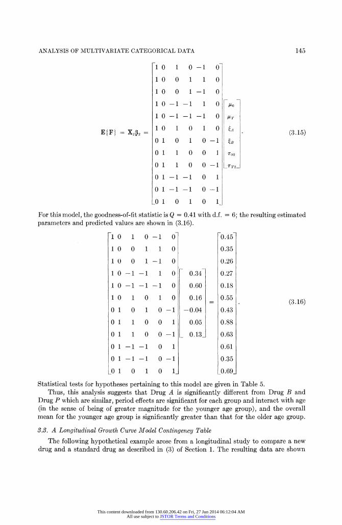
E{F} = X.32 = 1 0 1 0 1 0 A. (3.15) 0 1 0 1 0 -1 jB

0 1 1 0 0 1 T02

0 1 1 0 0 1 _Ty2-

01 -1 -1 0 1

0 1-1 -1 0 -I

_0 1 0 1 0 1_

For this model, the goodness-of-fit statistic is Q = 0.41 with d.f. = 6; the resulting estimated parameters and predicted values are shown in (3.16).

1 0 1 0 -1 0 0.45

1 0 0 1 1 0 0.35

1 ( 0 1 -1 0 0.26

1 0 -1 -1 1 0 7 0.34 0.27

1 0 -1 -1 -1 0 0.60 0.18

1 0 1 0 1 0 0.16 = 0.55 (3.16)

0 1 0 1 0 -1 -0.04 0.43

0 1 1 0 0 1 0.05 0.88

0 1 1 0 0 -1 0.13_ 0.63

0 1 -1 -1 0 1 0.61

0 1 -1 -1 0 -1 0.35

_01 0 1 0 1_ _0.69_

Statistical tests for hypotheses pertaining to this model are given in Table 5. Thus, this analysis suggests that Drug A is significantly different from Drug B and

Drug P which are similar, period effects are significant for each group and interact with age (in the sense of being of greater magnitude for the younger age group), and the overall mean for the younger age group is significantly greater than that for the older age group.

3.3. A Longitudinal Growth Curve Model Contingency Table The following hypothetical example arose from a longitudinal study to compare a new

drug and a standard drug as described in (3) of Section 1. The resulting data are shown





Hypothesis D.F. QC

CA = CB = 0 2 49.21

Po = lY 1 40.37

T02 = 0 1 4.81

TY2 = 0 1 31.16

T02 =Y2 1 6.37

2CA + B = = 1 47.55

A + 2B = ? B 1 3.68

CA =B 1 21.17

in Table 6. This experiment involves s = 4 sub-populations (2 diagnoses X 2 treatments), d = 3 conditions (week 1, week 2, week 4), and L = 2 response categories (normal N and abnormal A). Thus, there are r = Ld = 23 = 8 possible multivariate response profiles. The effects of diagnosis and treatment on a patient's condition over time is investigated by using the Al-matrix

1 1 110000

0000 1 1 1 1

Al = 1 1 00 1 1 00 014 (3.17)

00 1 1 00 1 1

1 0 1 0 1 0 1 0

_O 1 0 1 0 1 0 1_

to generate estimates for the first order marginal probabilities of normal (N) and abnormal (A) for each week vs. diagnosis vs. treatment combination and the A, matrix A, [1 -1]

Table 6 TABULATION OF RESPONSES FOR LONGITUDINAL STUDY

Response profile at week 1 vs week 2 vs week 4

Diagnosis Treatment NNN NNA NAN NAA ANN ANA AAN AAA Total

MilId Standard 16 13 9 3 14 4 15 6 80 Mild New drug 31 0 6 0 22 2 9 0 70 Severe Standard 2 2 8 9 9 15 27 28 100 Severe New drug 7 2 5 2 31 5 32 6 90

- ~ ~ 0111




0i 12 to generate their respective log ratios (or logits) as shown in Table 7 together with the corresponding estimated covariance matrix as shown in (3.18).

5.00 1.27 -0.76 1.27 5.16 -0.51

-0.76 -0.51 5.70 5.73 0.94 3.12 0.94 8.48 -1.87 (3.18) 3.12 -1.87 51.47

VF = 6.03 -0.56 0.08 X 10-2 -0.56 4.96 -0.38

0.08 -0.38 4.03 7.60 0.34 -0.81 0.34 4.44 0.18

-0.81 0.18 8.00_

Let X ti i denote the large sample expected value of the logit corresponding to the ilth diagnosis, i2th treatment and gth week. If time is assumed to represent a metric which reflects dosage of the drugs under study, then the linear logistic model with respect to log time represents a reasonable model by analogy to well-known results from existing methodology for quantal bio-assays as discussed by Berkson [1944, 1953, 1955] or Finney [1964]. More specifically, we consider the model (3.19)

il = 1: Mild, 2: Severe Xili2g = Aili2 + 'Yilixjlt2 i2 = 1: Standard, 2: New Drug (3.19)

g = 1: Week 1, 2: Week 2, 3: Week 4

where Aili2 represents an intercept parameter in reference to week 1 which is associated with ilth diagnosis and i2th treatment, 7y1j2 represents a corresponding continuous slope effect over time, and xtli., is the log to the base 2 of week, i.e., Xili2g = 0, 1, 2. In matrix notation, this model can be fitted via the regression model (3.20).

Table 7 OBSERVED AND PREDICTED ESTIMATES FOR FIRST ORDER MARGINAL

PROBABILITIES FOR NORMAL RESPONSE AND CORRESPONDING LOGITS

Observed Observed Predicted Predicted est. prob. Est. est. Est. est. Est. est. prob. Est.

Diagnosis Treatment Week normal s.e. logit s.e. logit s.e. normal s.e.

Mild Standard 1 0.51 0.06 0.05 0.22 -0.07 0.13 0.48 0.03 Mild Standard 2 0.59 0.06 0.35 0.23 0.42 0.11 0.60 0.03 Mild Standard 4 0.68 0.05 0.73 0.24 0.92 0.16 0.71 0.03 Mild New drug 1 0.53 0.06 0.11 0.24 -0.07 0.13 0.48 0.03 Mild New drug 2 0.79 0.05 1.30 0.29 1.38 0.15 0.80 0.02 Mild New drug 4 0.97 0.02 3.53 0.71 2.84 0.25 0.94 0.01

Severe Standard 1 0.21 0.04 -1.32 0.25 -1.35 0.13 0.21 0.02 Severe Standard 2 0.28 0.04 -0.94 0.22 -0.86 0.10 0.30 0.02 Severe Standard 4 0.46 0.05 -0.16 0.20 -0.36 0.15 0.41 0.04 Severe New drug 1 0.18 0.04 -1.53 0.27 -1.35 0.13 0.21 0.02 Severe New drug 2 0.50 0.05 0.00 0.21 0.10 0.12 0.53 0.03 Severe New drug 4 0.83 0.04 1.61 0.27 1.56 0.21 0.82 0.03




1 0

1 0 Y11

1 1 A 1 2

EA f} = = 1 2 721 (3.20) 1 0 /121

1 2 P222

1 0 -722-

12

for which the goodness-of-fit statistic is Q = 1.60 with d.f. = 4. The hypotheses and test statistics in Table 8 suggest differences exist among the respective diagnosis X treatment patient groups with respect to the intercept and slope parameters; and that such differences among the intercepts can be explained in terms of a diagnosis effect while such differences among the slopes can be explained in terms of a treatment effect. On the basis of these results, the original model can be simplified to the following

1 0 0 0

1 0 1 0

1 0 2 0

1 0 0 0

EAIf} = X252 = 1 0 0 2 A2* (3.21) 0 1 0 0 Y*1

0 1 2 0

0 1 0 0

0 1 0 1

_0 1 020

where ,i is an intercept parameter associated with the ilth diagnosis and 'Y*i, is a slope effect associated with the i~th treatment. For this model, the goodness-of-fit statistic is Q = 4.20 with U~. = S. The corresponding estimated parameter vector b, and its estimated covariance matrix Vb, are given in (3.22).





Hypothesis D.F. QC

1111 = l2 =>21 =2 3 44.47

Yll = 12 Y= 1 Y22 3 29.46

I1 I1 1 12 1 0.01

121 = 1122 1 0.17

yl = y2 1 1.29 Y1 1 Y2 111.2

Y12 Y22 1 0.16

-0.07 - 1.82 0.75 -0.74 -0.64

b2 = -1.35 , Vb2 = 0.75 1.82 -0.83 -1.04 X 10-2 (3.22) 0.49 -0.74 -0.83 0.93 0.53

_ 1.46_ L-0.64 -1.04 0.53 1.691

From these results, predicted logits as shown in Table 8 can be determined via (A.12). These can then be used to obtain the predicted values for the first order marginal probabilities of normal (N) responses by reverse transformation. These quantities are also shown in Table 7. Estimated standard errors for these predicted values obtained through suitable manipulations of (A. 13) are substantially smaller than those for the corresponding observed estimates, and thus reflect the extent to which the fitted model X2 enhances statistical efficiency. Finally, the hypotheses and test statistics in Table 9 justify the conclusions that the effects of diagnosis are significant but do not interact with time. Drug effects are also significant but are modulated in terms of different linear logistic trends over time. In other words, for both mild and severe diagnoses, a patient's condition becomes graded (N) sooner with the new drug than the standard drug even though there is essentially no difference between the treatments at the end of one week.


Hypothesis D.F. QC

1* ='2* 1 77. 02

Y*1 =Y*2 1 59.12

Y*1 = 0 1 26.35

Y*2 = 0 1 125.08




Acknowledgments This research was supported in part by National Institutes of Health, Institute of

General Medical Sciences through Grant GM-70004-05, by the U. S. Bureau of the Census through Joint Statistical Agreement JSA 75-2, and by Burroughs-Wellcome Co. through Joint Research Agreement 75-1.

The authors would like to thank Ms. Karen McKee and Ms. Rebecca Wesson for their cheerful and conscientious typing of the manuscript. The authors also wish to thank Ms. Linda L. Blakley and 1\is. Connie Massey for their competent typing of the tables and other manuscript revisions.

Une ]1Iethodologie Generale pour L'Analyse d'Experiences avec ]JIesures Repetees de Donnees en Categories

Resume

Cet article s'attache a l'analyse de donnees multivariates en categories, donnees obtenues a partir de mesures sur des experiences repetees. On fournit dans un expose introductif, les hypotheses pertinentes pour de telles situations, et on developpe les tests statistiques adapts en ap- pliquant la methode des moindres carries ponderes. On s'attarde tout particulierement sur pertains problernes de calcul lies a la manipulation de grands tableaux incluant le traitement de cellules vides. On fournit trois applications de cette methodologie.

References Anderson, R. L. and Bancroft, T. A. [1952]. Statistical Theory in Research. McGraw-Hill, New York,

Chapter 23. Berkson, J. [1944]. Application of the logistic function to bioassay. Journal of the American Statistical

Association 39, 357-365. Berkson, J. [1953]. A statistically precise and relatively simple method of estimating the bioassay

with quanta] response based on the logistic function. Journal of the American Statistical Associa- tion 48, 565-599.

Berkson, J. [1955]. Maximum likelihood and minimum X2 estimates of the logistic function. Journal of the American Statistical Association 50, 130-162.

Bhapkar, V. P. [1966]. A note on the equivalence of two test criteria for hypotheses in categorical data. Journal of the American Statistical Association 6, 228-235.

Bhapker, V. P. [1968]. On the analysis of contingency tables with a quantitative response. Biometrics 24, 329-338.

Bhapkar, V. P. and Koch, G. G. [1968a]. Hypotheses of 'no interaction' in multidimensional contingency tables. Technometrics 10, 107-123.

Bhapkar, V. P. and Koch, G. G. [1968b]. On the hypotheses of 'no interaction' in multidimensional contingency tables. Biometrics 24, 567-594.

Bishop, Y. M., Fienberg, S. E. and Holland, P. W. [1975]. Discrete Multivariate Analysis: Theory and Practice. M.I.T. Press, Cambridge, Massachusetts.

Bowker, A. H. [1948]. A test for symmetry in contingency tables. Journal of the American Statistical Association 43, 572-574.

Chen, T. and Fieinberg, S. E. [1974]. Two-dimensional contingency tables with both completely and partially cross-classified data. Biometrics 30, 629-642.

Cochran, W. [1950]. The comparison of percentages in matched samples. Biornetrika 37, 256-266. Cole, J. W. L. and Grizzle, J. E. [1966]. Application of multivariate analysis of variance to repeated

measurements experiments. Biometrics 22, 810-827. Davidson, R. R. and Bradley, R. A. [1969]. Multivariate paired comparisons: the extension of a

univariate model and associated estimation and test procedures. Biometrika 56, 81-95.




Federer, W. T. [1955]. Experimental Design: Theory and Application. Macmillan, New York, Chapter 10.

Fienberg, S. E. and Larntz, K. [1975]. Loglinear representation for paired and multiple comparisons models. Biometrika G3, 245-254.

Finney, D. J. [1964]. Statistical Method in Biological Assay, 2nd ed., Griffin, Ltd., London. Forthofer, R. N. and Koch, G. G. [1973]. An analysis for compounded functions of categorical data.

Biometrics 29, 143-157. Grizzle, J. E. [1965]. The two-period change-over design and its use in clinical trials. Biometrics 21,

467-480. Grizzle, J. E., Starmer, C. F. and Koch, G. G. [1969]. Analysis of categorical data by linear models.

Biometrics 25, 489-504. Hocking, R. R. and Oxspring, H. H. [1974]. The analysis of partially categorized contingency data.

Biometrics 30, 469-483. Imrey, P. B., Johnson, W. D. and Koch, G. G. [1975]. An incomplete contingency table approach

to paired-comparison experiments. Journal of the American Statistical Association 71, 614-623. Koch, G. G. [1969]. Some aspects of the statistical analysis of 'split plot' experiments in completely

randomized layouts. Journal of the American Statistical Association 64, 485-505. Koch. G. G. [1970]. The use of non-parameteric methods in the statistical analysis of a complex split

plot experiment. Biometrics 26, 105-128. Koch, G. G. [1972]. The use of non-parametric methods in the statistical analysis of the two-period

change-over design. Biometrics 28, 577-584. Koch, G. G., Abernathy, J. A and Imrey, P. B. [1975]. On a method for studying family size pref-

erences. Demography 12, 57-66. Koch, G. G., Freeman, J. L., Freeman, D. H., Jr. and Lehnen, R. G. [1974]. A general methodology

for the analysis of experiments with repeated measurement of categorical data. University of North Carolina Institute of Statistics Mimeo Series No. 961.

Koch, G. G., Freeman, J. L. and Lehnen, R. G. [1976]. A general methodology for the analysis of ranked policy preference data. International Statistical Review 44, 1-28.

Koch, G. G., Imrey, P. B., Freeman, D. H., Jr. and Tolley, H. D. [1976]. The asymptotic covariance structure of estimated parameters from contingency table log-linear models. Proceedings of the 9th International Biometric Conference, 317-336.

Koch, G. G., Imrey, P. B. and Reinfurt, D. W. [1972]. Linear model analysis of categorical data with incomplete response vectors. Biometrics 28, 663-692.

Koch, G. G. and Reinfurt, D. W. [1971]. The analysis of categorical data from mixed models. Bio- metrics 27, 157-173.

Koch, G. G., Johnson, W. D., and Tolley, H. D. [1972]. A linear models approach to the analysis of survival and extent of disease in multidimensional contingency tables. Journal of the American Statistical Association 67, 783-796.

Koch, G. G. and Tolley, H. D. [1975]. A generalized modified X2 analysis of data from a complex serial dilution experiment. Biometrics 31, 59-92.

Kullback, S. [1971]. Marginal homogeneity of multidimensional contingency tables. Annals of Math Statistics 42, 594-606.

Landis, J. R. [1975]. A general methodology for the measurement of observer agreement when the data are categorical. Ph.D. Dissertation, University of North Carolina Institute of Statistics Mimeo Series, No. 1022.

Landis, J. R. and Koch, G. G. [1975a]. A review of statistical methods in the analysis of data arising from observer reliability studies (Part I). Statistica Neerlandica 29, 101-123.

Landis, J. R. and Koch, G. G. [1975b]. A review of statistical methods in the analysis of data arising from observer reliability studies (Part II). Statistica Neerlandica 29, 151-161.

Landis, J. R. and Koch, G. G. [1977a]. The measurement of observer agreement for categorical data. Biometrics 33, 159-175.

Landis, J. R. and Koch, G. G. [1977b]. An application of hierarchical kappa-type statistics in the assessment of majority agreement among multiple observers. University of Michigan Biostatistics Technical Report No. 13. To appear in Biometrics.

Landis, J. R. and Koch, G. G. [1977c]. The analysis of categorical data in longitudinal studies of behavioral development. To appear in Manual on Longitudinal Research Methodology, a technical report, J. R. Nesselroade and P. B. Baltes, (eds.), for the National Institute of Education.




Landis, J. R., Stanish, W. M., Freeman, J. L. and Koch, G. G. [1976]. A computer program for the generalized chi-square analysis of categorical data using weighted least squares (GENCAT). University of Michigan Biostatistics Technical Report No. 8. To appear in Computer Programs in Biomedicine.

Lehnen, R. G. and Koch, G. G. [1974a]. Analyzing panel data with uncontrolled attrition. The Public Opinion Quarterly 38, 40-56.

Lehnen, R. G. and Koch, G. G. [1974b]. The analysis of categorical data from repeated measurement research designs. Political Methodology 1, 103-123.

Morrison, D. F. [1967]. Mlultivariate Statistical Methods. McGraw-Hill, New York, Chapters 4 and 5. Neyman, J. [19491. Contribution to the theory of the X2 test. Proceedings of the Berkeley Symposium

on Mathematical Statistics and Probability. Berkeley and Los Angeles: University of California Press, Berkeley and Los Angeles, (239-272).

Steel, R. G. D. and Torrie, J. H. [1960]. Principles and Procedures of Statistics. McGraw-Hill, New York, Chapter 12.

Wald, A. Tests of statistical hypotheses concerning general parameters when the number of observa- tions is large. Transactions of the American Mathematical Society 54, 426-482.

Received July 1975, Revised May 1976

Appendix 1

General Framework

The purpose of this appendix is to restate the general framework for the methodology originally outlined in Grizzle, Starmer and Koch [1969] with emphasis directed at:

i. additional clarification of the relationship between model fitting and hypothesis testing in terms of the relationship between goodness-of-fit statistics and contrast matrix test statistics;

ii. additional clarification of the Central Limit Theory justification for weighted least square model fitting procedures;

iii. additional aspects of analysis like predicted functions and their corresponding estimated covariance matrix;

iv. coverage of a broader class of functions beyond linear and log-linear functions.

This appendix also expresses why marginal probability functions and/or mean scores can be effectively analyzed for moderate size repeated measurement experiments which involve large tables with sparse data within the scope of weighted least squares methods but not necessarily maximum likelihood methods (which require attention to be directed at the set of joint cell probabilities in the overall table).

Let g = 1, 2, * *, d index the d conditions under which measurements on the same basic response with L categories are observed. Let j = 1, 2, * , r index the set of categories which correspond to the r = Ld response profiles associated with the simultaneous classification for the d responses of interest. Similarly, let i = 1, 2, *, s index a set of categories which correspond to distinct sub-populations as defined in terms of pertinent independent variables. If samples of size ni where i = 1, 2, * * *, s are independently selected from the respective sub-populations, then the resulting data can be summarized in an (s X r) contingency table as shown in Table 10, where n j denotes the frequency of response category j in the sample from the ith sub-population.

The vector ni where ni' = (nil, ni2, *, nir) will be assumed to follow the multinomial distribution with parameters ni and =i' = (7ril, ri2, rir), where 7rij represents the probability that a randomly selected element from the ith population is classified in the jth response category. Thus, the relevant product multinomial model is

f l3ni! fl[7ri,?i"/nii!], (A. 1) i=1 ____

with the constraints

E ri= 1 for i = 1, 2, . , s. (A.2) 3 1




Table 10 OBSERVED CONTINGENCY TABLE

Response profile categories Sub-population

1 2 ... r Total

1 n 11 n12 ... nlr n1

2 n21 n22 ... n2r n2

S n5i ns2 ... n n sl s2 ~~ ~~sr s

Let pi = (ni/ni) be the (r X 1) vector of observed proportions associated with the sample from the ith sub-population and let p be the (sr X 1) compound vector defined by p' = (PI', P2', * , p/'). Thus, the vector p is the unrestricted maximum likelihood estimator (MLE) of = where =' = =2 f2', , as'). A consistent estimator for the covariance matrix of p is given by the (sr X sr) block diagonal matrix V(p) with the matrices

V, (pi) = [Dp, - pipi'] (A.3) (rXr) ni

for i = 1, 2, * * s on the main diagonal, where Dph is an(r X r) diagonal matrix with elements of the vector pi on the main diagonal.

Let F1(p), F2(p), * *, F,(p) be a set of u functions of p which pertain to some aspect of the relationship between the distribution of the response profiles and the nature of the sub-populations. Each of these functions is assumed to have continuous partial derivatives through order two with respect to the elements of p within an open region containing = = E {p }. If F _ F(p) is defined by

F' = [F(p)]' = [F1(p), F2(P), --, Fu(p)], (A.4)

then a consistent estimator for the covariance matrix of F is the (u X u) matrix

VF = H[V(p)]H', (A.5)

where H = [dF(x)/dx I x = p] is the (u X sr) matrix of first partial derivatives of the functions F evaluated at p. In all applications, the functions comprising F are chosen so that VF is asymptotically nonsingular.

The function vector F is a consistent estimator of F(=). Hence, the variation among the elements of F(=) can be investigated by fitting linear regression models by the method of weighted least squares. This phase of the analysis can be characterized by writing

EA{F } = EA{F(P)} = F(n) = X (A.6) where X is a pre-specified (u X t) design (or independent variable) matrix of known coefficients with full rank t < u, 5 is an unknown (t X 1) vector of parameters, and "EA" means "asymptotic expectation".

An appropriate test statistic for the goodness-of-fit of the model (A.6) is

Q = Q(X, F) = (RF)'[RVFR']-1RF, (A.7) where R is any full rank [(u - t) X u] matrix orthogonal to X. Here Q is approximately distributed according to the x2 distribution with d.f. = (u - t) if the sample sizes Ini} are sufficiently large that the elements of the vector F have an approximate multivariate normal distribution as a consequence of Central Limit Theory (CLT). Test statistics such as Q are known as generalized Wald [1943] statistics and various aspects of their application to a broad range of problems involving the analysis of multivariate categorical data are discussed in Bhapkar and Koch [1968a, 1968b] and in GSK [1969].

However, these test statistics like (A.7) are obtained in actual practice by using weighted least squares




as a computational algorithm which is justified on the basis of the fact that Q of (A.7) is identically equal to

Q = (F - Xb)'VF-(F - Xb) (A.8)

where b = (X'VF-'X)-'X'VF- F is a BAN estimator for 5 based on the linearized modified x 2-statistic of Neyman [1949]. In view of this identity demonstrated in Bhapkar [1966], both Q and b are regarded as having reasonable statistical properties- in samples which are sufficiently large for applying CLT to the functions F. As a result, a consistent estimator for the covariance matrix of b is given by

Vb = (X'VF1X)1. (A.9)

If the model (A.6) does adequately characterize the vector F(=), tests of linear hypotheses pertaining to the parmeters 0 can be undertaken by standard multiple regression procedures. Ill particular, for a general hypothesis of the form,

Ho =Q 0, (A.l1)

where C is a known (c X t) matrix of full rank c < t and 0 is a (c X 1) vector of 0's, a suitable test statistic is

Qc = (Cb)'[C(X'VF-1X)-C']1-'Cb (A.ll) which has approximately a x 2 -distribution with d.f. = c in large samples under Ho in. (A. 10).

In this framework, the test statistic Qc reflects the amount by which the goodness-of-fit statistic (A.8) would increase if the model (A.6) were simplified (or reduced) by substitutions based on the additional constraints implied by (A. 10). Thus, these methods permit the total variation within F(=) to be partitioned into specific sources and hence represent a statistically valid analysis of variance for the corresponding estimator functions F.

Predicted values for F(=) based on the model (A.6) can be calculated from

F = Xb = X(X'VF- X) -X'VF-'F. (A.12)

Thus, consistent estimators for the variances of the elements of F can be obtained from the diagonal elements of

VPw= X(X'VF_1X)-1X'. (A.13)

The predicted values f not only have the advantage of characterizing essentially all the important features of the variation in F(=), but also represent better estimators than the original function statistics F since they are based on the data from the entire sample as opposed to its component parts. Moreover, they are descriptively advantageous in the sense that they make trends more apparent and permit a clearer interpretation of the relationship between F(=) and the variables comprising the columns of X.

Although the formulation of F(p) can be quite general, GSK [1969] and Forthofer and Koch [1973] demonstrated that a wide range of problems in categorical data analysis could be considered within the framework of a few specified classes of compounded logarithmic, exponential and linear functions of the observed proportions. However, these functions are all special cases of a broad class of functions which can be expressed in terms of repeated applications of any sequence of the following matrix operations:

(i) Linear transformations of the type

Fi(p) = Alp = al, (A.14) where A, is a matrix of known constants;

(ii) Logarithmic transformations of the type

F2(p) = loge (p) = a2 , (A.15) where loge transforms a vector to the corresponding vector of natural logarithms;

(iii) Exponential transformations of the type

F3(p) = exp (p) = a3, (A.16)

whcre exp transforms a vector to the corresponding vector of exponentialfunctions, i.e., of antilogarithnis.




Then the linearized Taylor-series-based estimate of the covariance matrix of FkW for ik = 1, 2, 3, is given by (A.5), where the corresponding Hk matrix operator is

H1 = A1; (A.17)

H2= D= (A.18)

H3 = Da3 , (A.19) where Dy is a diagonal matrix with elements of the vector y on the main diagonal.

The hypotheses involving marginal distributions can all be tested in terms of linear functions of the form given in (A. 14). Furthermore, compounded logarithmic-exponential-linear functions of the form

F(p) = exp [A4(10ge {A3[exp A2 {1 oge [Alp]})]})] (A.20) can be used to generate complex ratio estimates such as generalized kappa-type statistics described in Landis and Koch [1977a, 1977b]. As a result, the linearized Taylor-series-based estimate of the covariance matrix associated with F(p) in (A.20) can be obtained by repeated application of the chain rule for matrix differentiation. In particular, let

a, = Alp; (A.21)

a2 = exp {A2 [loge (a,)]}; (A.22)

a3 = A3a2 ; (A.23)

a4 = exp {A4 [log (a3)]}. (A.24)

Then the results in (A.17)-(A.19) can be used to provide a consistent estimate of the covariance matrix via (A.5) by using

H = Da.A4Da3 'ADaA2DajAi (A.25) Since the methods of analysis described here are based on asymptotic considerations, the functions

F(p) must be chosen carefully so as to support the inherent assumption that the statistical behavior (i.e., expected values and covariance structure) of such functions is approximately characterized by their linearized Taylor series counterparts. However, by virtue of the uniqueness of the Taylor series with respect to p, the reader should realize that this issue pertains to the inherent nature of such functions rather than to the complexity of their compounded function representation via (A.20). As stated previously, the primary purpose of (A.2) is the computational convenience achieved for (A.25) by such simplistic operations as matrix multiplication, diagonal matrix inversion, loge and exp. Thus, although the complexity of (A.20) should be a source of concern regarding the use of asymptotic methods, it should not dominate such decisions, but rather should call attention to the necessity of alternative arguments for justifying the applicability of the linearized Taylor series approximations. Examples where such justification can be given for moderately large sample sizes include the Goodman-Kruskal rank correlation coefficients (see Forthofer and Koch [19733), life-table based survival rates (see Koch, Johnson and Tolley [1972]), and generalized kappa type measures of agreement (see Landis and Koch [1977a]). On the other hand, for those situations where the linear Taylor series approximation is not valid but Central Limit Theory arguments are still appropriate with respect to F(p), then other procedures (e.g., Jack-knife methods) should be used to obtain the required consistent estimator for the covariance structure of F, and the weighted least squares aspects of the analysis (A.6)-(A.13) can proceed as previously described with no loss of generality.

Koch, Imrey, Freeman and Tolley [1976] discuss the application of this general approach to implicitly defined functions of p in the context of estimated parameters from fitted log-linear models. All aspects of this methodology can be directed at implicit functions which are based on maximum likelihood estimation equations corresponding to preliminary or intermediate (as opposed to final) models with a priori assumed validity; in other words, models in which the likelihood (A.1) initially, i.e., prior to any data analysis, satisfies both (A.2) as well as certain other constraints analogous to (A.6).

For purposes of completeness, it should be noted that other statistical procedures for the analysis of categorical data from repeated measurement experiments are available in the literature. Bishop, Fienberg and Holland [1975, Chapter 8] discuss the application of maximum likelihood methods to test hypotheses of total symmetry and marginal symmetry as well as certain other hypotheses of interest. They also provide




a complete literature review of other papers dealing with similar questions including the early work of Bowker [1948] and Cochran [1950] as well as the minimum discrimination information approach of Kullback [1971]. However, all of these methods are intimately connected to the product multinomial model (A.1) which involves the joint probability = and the observed frequency vector n. Thus, for applications involving large tables, e.g., d > 4, L > 4, so that r = Ld > 256, the sample sizes required for their statistical validity may be considerably larger than those required for the weighted least squares estimators which are directed at the first order marginal probabilities {fink } or mean scores { 7i j}. Moreover, they may also require a pro- hibitively greater amount of computational effort in such situations because they involve the manipulation of the full (s X r) contingency table. On the other hand, this difficulty can be bypassed with the approach presented in this paper by constructing the estimators F for the first order marginal probabilities {1i9k and mean scores t?7i,} directly from the observed raw data for each subject (as opposed to the corresponding contingency table) by the indicator function operations described in Appendix 2. For these reasons, weighted least squares oriented methods may often provide more effective analyses than maximum likelihood oriented methods for repeated measurement experiments with categorical data, particularly for those involving large underlying contingency tables with sparsely distributed samples.

Appendix 2

Special Considerations for Large Tables and Zero Cells

Unless both the number of conditions d and the number of response categories L are small, e.g., d < 3, L < 3, the number of possible multivariate response profiles r = Ld can become very large. In this event, there are two sources of potential difficulty:

i. The manipulation of very large contingency tables and operator matrices can involve expensive computations.

ii. For each sub-population i = 1, 2, **, s, some of the r possible response profiles j will not necessarily be observed so that the corresponding cellfrequencies nij are zero.

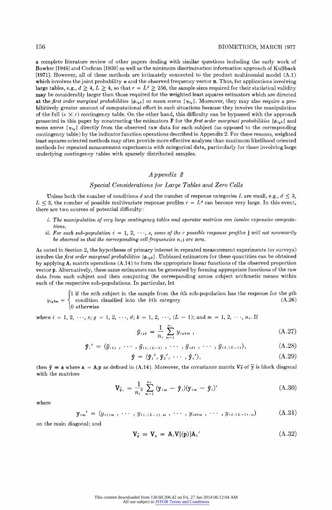
As noted in Section 2, the hypotheses of primary interest in repeated measurement experiments (or surveys) involve the first order marginal probabilities {1igk}. Unbiased estimators for these quantities can be obtained by applying Al matrix operations (A.14) to form the appropriate linear functions of the observed proportion vector p. Alternatively, these same estimators can be generated by forming appropriate functions of the raw data from each subject and then computing the corresponding across subject arithmetic means within each of the respective sub-populations. In particular, let

1 if the mth subject in the sample from the ith sub-population has the response for the gth Yigkm= condition classified into the kth category (A.26)

t0 otherwise

where i = 1, 2, ,s; g = 1, 2, **,d; k = 1, 2, **, (L - 1); and m = 1, 2, *,n. If

1 ni

Yigk = Yiokm , (A.27) him=1

Yi = (gill il,(L-) Yil, , (-)) A.28)

= (YS', Y2, , Y8'), (A.29) then y-a where a = Alp as defined in (A.14). Moreover, the covariance matrix V- of y is block diagonal with the matrices

1 fli

Vi= n _2 (yin -Yi)(Y -

YX (A.30)

where

yips = (Yilll, , Yil ,(-1), , Yidlmn, , Yi(i (i-i) a) (A.31) on the main diagonal; and

V- Va = AV[(p)]Al' (A .32)




as given in (A.5) with (A.17). Since sd(L - 1) is usually moderate in size, this method of computation of the estimators for the first order marginal probabilities is reasonably straightforward and efficient. Moreover, it can be similarly applied to compute mean scores based on quantitative scales a,, a2, * * *, aL for ordinal responses. Finally, as indicated in Landis, Stanish, Freeman and Koch [19761, these operations can be readily linked with other algorithms for performing logarithmic and exponential operations as shown in (A.15)-(A.20) as well as weighted least squares regression analysis. Thus, this computational strategy represents an effective way of dealing with (i). Examples which illustrate its application are given in Koch, Freeman and Lehnen [19761 and Landis and Koch [1977b].

For repeated measurement experiments, the potential tendency for some of the ni to be zero does not cause any real problems except when such zero frequencies induce singularities in the estimated covariance matrix VF in (A.5) for the function vector F which is to be analyzed, or otherwise restrict the extent to which CLT arguments can be applied to the distribution of F. With respect to the hypotheses Hsj and HCJ, CLT arguments cannot be applied with confidence to the estimators pii = (nii/nt) of the 7ri unless most of the nsi > 5.

This condition, however, is usually not satisfied for situations involving moderately large samples, ni > 100, except when both L and d are small, i.e., d < 3, L < 3. Thus, in such cases, the potential presence of many zero frequencies implies that these hypotheses cannot be validly tested by the general inethodo- logical approach given in this paper.

On the other hand, if attention can be restricted to hypotheses like HSM and HCM1I or HSAAI and HCAM, which involve the first order marginal probabilities {1 } 1, then the sample size requirements are considerably less severe. In particular, CLT can be applied with reasonable validity to estimates of the {1igk} obtained either by Al matrix operations like (A.14) or by direct computations like (A.27) provided the overall within sub-population sample sizes ni > 25 and most of the first order marginal frequencies

nilk = X,... * ?i, i i -- -',j > 5 (A.33) j wvi th ig=k

Since Ek=lL niQk = ni, the conditions (A.33) tend to hold in most situations where the sample sizes ni > 25 and where the number of response categories is small, i.e., L < 3.

However, if L is not small, then cases where (A.33) tends not to hold can be handled by pooling certain response categories together so that (A.33) is satisfied by the pooled frequencies. Of course, attempts should be made to base such pooling on conceptual similarities among the response categories as well as to prevent such pooling from masking any obvious differences among either sub-populations or among conditions. Otherwise, the logical relationship between the interpretation of the hypotheses Hsm (or HcAI) for the pooled categories vs. the original categories is analogous to the logical relationship between HSAM (or HCAM.1) and HKs'M (or HCM). Alternatively, many of the situations where L is large involve ordinally scaled response categories, and hence, the quantities of interest are estimates of mean score functions { -qni }. CLT can be applied with reasonable validity to these statistics provided the overall within sub-population sample sizes ni > 25, and the corresponding observed response distributions for each measurement condition are not degenerate in the sense of being concentrated in a single response category. This latter requirement is satisfied for most purposes if there exist response categories k(i, g) for each sub-population x condition combination such that,

k (i, v) I'

E ni,, > 5, ni 01 > 5. (A.34) k~~~~~~~i ~ ~ ~ ~ +1 ) 1 = 1 I =~~~~~ ( A ( i ,ua) +l)

The previous remarks deal with the extent to which the presence of zero frequencies affects the types of functions to which CLT arguments can be applied in a valid manner. Moreover, when such functions are chosen judiciously, the resulting estimated covariance matrix VF usually will be nonsingular. However, if VF is singular, then a number of technical difficulties arise in applying the Appendix 1 methodology because matrix inversion of VF can no longer be performed. For these situations, the vector F can be analyzed by the Appendix 1 methodology provided that the estimated covariance matrix VF is replaced by a suitably similar, nonsingular, pseudo estimated covariance matrix VF*.

If both L and d are small, e.g., d < 3, L < 3, such a nonsirngular matrix VF* can be obtained by applying the same operations used to form VF to the pseudo full (s X r) contingency table in which some of the "0" frequencies are replaced by an appropriate small number like "(1/2)." The motivation behind this is the findings of Berkson [19551 who investigated its effects on estimation involving the logit, i.e., natural logarithm of the ratio of the proportions, associated with r = 2 responses. For the case where r = Ld is large, the properties of this rule are largely unknown; and thus the recommendation here is not to replace




all "0" frequencies by (1/2), but to modify only those which are necessary to the construction of a nonsingular estimated covariance matrix VF* for F. Other aspects of the analysis of F then proceed as described in Appendix 1, except that VF* is used as the estimated covariance matrix instead of VF.

The previously described method for constructing VF* is not practical when d > 4, L > 4 because the full contingency table is too large to manipulate efficiently. Moreover, in these cases, attention is primar- ily directed at the hypotheses pertaining to the first order marginal probabilities {i4k } for which unbiased estimators {Yik} are determined via (A.26) and (A.27) and the corresponding estimated covariance matrix Vy is determined via (A.30). Unfortunately, if Vy is singular, considerable effort may be required to construct a nonsingular, pseudo estimated covariance matrix VY* for y. For this purpose, the basic strategy is to augment the raw data for the respective subjects with pesudo data vectors with smaller weights like (1/2) until the required nonsingular matrix Vy* is determined. For further discussion, see Koch, Freeman, Freeman, and Lehnen [1974].

In summary, questions pertaining to zero cells and singularities are best resolved by statistical j udg- ments which take into account the special features of each experimental (or survey) situation where such methods are applied. For many situations, this can be accomplished by restricting attention to hypotheses involving the first order marginal probabilities {y ink} (or mean scores { -qig 1). In other cases, the use of modular MLEs as discussed in Koch and Tolley [1975] and Koch, Imrey, Freeman and Tolley [19761 may be required to "smooth" away the singularities in VF through the assumption of certain a priori constraints on the likelihood (A. 1). However, if singularities are still present, then the analysis of F can often be effectively undertaken through the use, with appropriate caution, of a non-singular, pseudo estimated covariance matrix VF*.



a general methodology for the analysis of experiments with repeated measurement of categorical data

Documents