a galerkin least squares finite element method for the two dimensional helmholtz equation
TRANSCRIPT
A Galerkin Least Squares Finite Element Methodfor the Two-Dimensional Helmholtz Equation
Lonny L. Thompson and Peter M. Pinsky
Department of Civil Engineering, Stanford UniversityStanford, California 94305-4020
Abstract
In this paper a Galerkin least squares (GLS) finite element method, in whichresiduals in least-squares form are added to the standard Galerkin variationalequation, is developed to solve the Helmholtz equation in two-dimensions. Animportant feature of GLS methods is the introduction of a local mesh pa-rameter that may be designed to provide accurate solutions with relativelycoarse meshes. Previous work has accomplished this for the one-dimensionalHelmholtz equation using dispersion analysis. In this paper, the selection of theGLS mesh parameter for two-dimensions is considered, and leads to elementsthat exhibit improved phase accuracy. For any given direction of wave propa-gation, an optimal GLS mesh parameter is determined using two-dimensionalFourier analysis. In general problems, the direction of wave propagation willnot be known a priori. In this case, an optimal GLS parameter is found whichreduces phase error for all possible wave vector orientations over elements.The optimal GLS parameters are derived for both consistent and lumped massapproximations. Several numerical examples are given and the results com-pared with those obtained from the Galerkin method. The extension of GLSto higher-order quadratic interpolations is also presented.
International Journal for Numerical Methods in Engineering
Vol.38, pp. 371-397 (1995) (Received 23 August 1993; Revised 8 March 1994)
1
Two-Dimensional Helmholtz Equation 2
1 Introduction
Boundary-value problems governed by the Helmholtz equation are important in avariety of applications involving time-harmonic wave propagation phenomena suchas linear acoustics and electrodynamics. There is also interest in the Helmholtzequation in an abstract setting because of the potential for a loss of ellipticity (strongcoercivity) with increasing wavenumber. This difficulty is especially important whensolving large-scale problems with iterative solvers where the condition number of thematrix equations depends on the wavenumber, Bayliss, et. al. [1].Finite element solutions to the Helmholtz equation in two-dimensions have been
primarily sought using the standard Galerkin method; see for example, Maccamy andMarin [2], Goldstein [3], Bayliss, Goldstein and Turkel [4]. However, it is well knownthat the numerical phase accuracy of standard Galerkin finite element solutions de-teriorate rapidly as the wavenumber, normalized with the element mesh parameter,is increased, Belytschko and Mullen [5], Mullen and Belytschko [6]. This resolutionproblem arises from the use of piecewise polynomial shape functions to approximatehighly oscillatory wave propagation solutions. To obtain an acceptable level of accu-racy, more than ten elements per wavelength are required. For large wavenumbers,refining the mesh to maintain this requirement may become prohibitively expensive.Global error estimates based on the wavenumber and local element parameter forthe Galerkin finite element method are reported in Bayliss, et.al. [7], Aziz et.al. [8],Douglas et.al. [9], and Ihlenburg and Babuska [10].Several approaches designed to improve the numerical phase accuracy of the stan-
dard Galerkin method have been proposed in recent years. Goldstein [11] employed aversion of the weak element method to the Helmholtz equation where the local solu-tion within each element is approximated by a sum of exponentials. In this approach,continuity at interelement boundaries is enforced weakly for certain functionals ofthe approximate solution. As reported by Goldstein, for general problems in two-dimensions, the success of this approach has been limited.Park and Jensen [12] and Alvin and Park [13] used discrete Fourier analysis to
derive wavenumber dependent modifications to the stiffness and mass matrices arisingfrom standard Galerkin finite element methods. The modified element matrices aredesigned to minimize dispersion error over a specified frequency–wavenumber window.This approach can be viewed as an extension of previous modifications to Galerkinfinite element equations such as diagonal, and higher-order mass approximations,Goudreau and Taylor [14] and Fried [15], but now tailored over a specified rangeof frequencies. A difficulty of such methods, is that they do not possess a firmmathematical basis for proving stability and convergence. In particular, they do notinherit the consistency inherent in the Galerkin method, an important ingredient forobtaining improved convergence rates with higher-order interpolation functions.Over the last view years, a new class of residual based finite element formulations
has emerged to counteract the stability problems and other numerical pathologies ex-
Int. J. Numer. Meth. Engng., Vol.38, pp. 371-397 (1995)
Two-Dimensional Helmholtz Equation 3
hibited by the classical Galerkin method. These methods are developed by append-ing residuals of the Euler-Lagrange equations to the standard Galerkin variationalequation. The added residual terms preserve the consistency inherent in the par-ent Galerkin method. Methods of this type were originally developed by Hughes andBrooks [16], to improve the stability of numerical solutions for the advection-diffusionequation, and are referred to as ‘streamline-upwind/Petrov-Galerkin’ (SUPG) meth-ods. For a review of SUPG type methods applied to advective-diffusive systems andfluid flow equations, see Hughes [17] and Johnson [18].These ideas have since been extended by Hughes, Franca and Hulbert [19], to the
concept of Galerkin least-squares (GLS) by appending residuals of the Euler-Lagrangeequations in least-squares form to the standard Galerkin formulation. GLS finiteelement methods have been successfully employed in a wide variety of applicationswhere enhanced stability and accuracy properties are needed, including problemsgoverned by Navier-Stokes and the compressible Euler equations of fluid mechanics,Shakib and Hughes [20].Recently, Harari and Hughes [21] have applied Galerkin least-squares technology
to the Helmholtz equation for one-dimensional model problems. An important featureof GLS methods is the introduction of a local mesh parameter into the variationalequation that may be designed to provide accurate solutions with relatively coarsemeshes. Harari and Hughes accomplished this for one-dimensional problems usingdispersion analysis. In the paper by Harari and Hughes [22], the GLS mesh parameterderived in one-dimension is used in the DtN finite element method proposed by Kellerand Givoli [23] for solving the exterior Helmholtz problem. Although it was foundthat the one-dimensional parameter improved the accuracy of the Galerkin solution insome two-dimensional example problems, a comprehensive analysis of GLS dispersioncharacteristics in two-dimensions was unavailable.In this paper the selection of the optimal GLS mesh parameter for the two-
dimensional Helmholtz equation is considered, and leads to elements that exhibitimproved phase accuracy. Although for any given direction of wave propagation, itis shown in this paper that an optimal GLS mesh parameter can be obtained, ingeneral, the direction of wave propagation will not be known a priori. To remedy thisdifficulty, a GLS parameter is found which reduces phase error for all possible wavevector directions over an element. By performing a two-dimensional Fourier analysiswe have been able to characterize the phase accuracy and directional properties ofthe Galerkin least-squares solution over all wave vector magnitudes and directions. Anumber of alternative GLS parameters are derived for general numerical integrationrules such as Gaussian and Lobatto quadrature and their dispersion characteristicsanalyzed over the full range of wave vector orientations. Results from this analysisquantify the reduction in phase error achieved using alternative GLS mesh parame-ters.Extensions of GLS to higher-order finite element interpolations is also considered.
In particular, optimal GLS parameters designed to reduce dispersion for elements
Int. J. Numer. Meth. Engng., Vol.38, pp. 371-397 (1995)
Two-Dimensional Helmholtz Equation 4
with quadratic interpolation functions are derived together with some simple approx-imations useful for efficient computation. A number of example problems are numer-ically solved to verify the accuracy of the GLS method and assess the performance ofcompeting GLS design parameters.In Section 2 the Helmholtz equation and its characteristic equation relating fre-
quency and wave vector components in two-dimensions is reviewed. In Section 3the Galerkin least-squares variational equations are stated and difference equationsarising from the assembly of a uniform discretization of bilinear elements derived. InSection 4 a two-dimensional Fourier analysis of these equations is performed to ob-tain GLS dispersion relations. Optimal GLS parameters are derived and dispersioncurves compared to the standard Galerkin method in Section 5. In Section 6, numer-ical examples of both interior and exterior problems are solved. Finally, in Section 7extensions to higher-order quadratic finite elements are developed.
2 Helmholtz equation in two dimensions
Consider a two-dimensional homogeneous isotropic medium whose wave speed is c.The wave solution φ(x) corresponding to a harmonic source f vibrating at a givenfixed frequency ω > 0 satisfies the scalar Helmholtz equation:
Lφ ≡ ∇2φ+ k2φ = −f in Ω (1)
where k = ω/c > 0 is the wavenumber with wavelength 2π/k, ∇2 is the Laplaciandifferential operator and Ω is the spatial domain of interest. The Helmholtz equationis sometimes called the reduced wave equation, and plays a fundamental role in manymathematical models of physical phenomena including acoustics and electromagneticwave propagation. For example, in linear acoustics φ might represent a perturbationin pressure about a reference state.The Helmholtz equation in R2 admits the plane-wave propagating solution,
φ(x, y) = ei(kxx+kyy) (2)
where ω and the wave vector components kx and ky are linked by the characteristicequation,
(ωh
c
)2= (kxh)
2 + (kyh)2 (3)
and h is a problem dependent characteristic length. This nondispersive relation issatisfied by the directional wave vector components kx = k cos θ and ky = k sin θ,where the normal to the plane wave is oriented at angle θ relative to the x-axis.Alternatively, the characteristic equation (3) can be obtained by a two-dimensional
Fourier transform from physical space to wave space through the transform operation,
F (kx, ky) :=1√2π
∫ ∞−∞
∫ ∞−∞
F (x, y)e−i(kxx+kyy)dxdy (4)
Int. J. Numer. Meth. Engng., Vol.38, pp. 371-397 (1995)
Two-Dimensional Helmholtz Equation 5
The discrete counterpart to this continuous transform will be used as a tool for thedesign of improved finite element methods for the solution of the two-dimensionalHelmholtz equation.
3 Finite Element Formulations
Consider a partition of Ω into finite elements. Let Ωe be the interior of the ethelement, and Ω =
⋃eΩe. Let S
h ⊂ H1(Ω) and Vh ⊂ H1(Ω) be finite element spacesconsisting of continuous piecewise polynomials of order p.
3.1 Galerkin
As a point of departure, consider the classical Galerkin method.Given k = ω/c > 0, find φh ∈ Sh, such that
A(wh, φh) = L(wh) ∀wh ∈ Vh (5)
where
A(wh, φh) ≡ (∇wh,∇φh)Ω − k2(wh, φh)Ω (6)
L(wh) ≡ (wh, f)Ω (7)
and (·, ·)Ω denotes the L2(Ω) inner product. The Galerkin formulation is consistentin the sense that φ, the exact solution to the Helmholtz equation, satisfies (5). Fork2 > 0 the operator,
A(wh, wh) = ||∇wh||2 − k2||wh||2 ∀wh ∈ Vh (8)
loses positive-definiteness as the wavenumber increases, and stability may be degradedfor large k.
3.2 Galerkin/least-squares
It is well known that the phase accuracy associated with the Galerkin finite elementsolution degrades as the wavenumber k is increased relative to the mesh parameterh. In order to improve accuracy characteristics of the standard Galerkin method, aleast-squares operator is added to (5). This additional operator is constructed froma residual of the governing Helmholtz differential equation evaluated within elementinteriors.
A(wh, φh) + (τLwh, rh)Ω = L(wh) (9)
In this expression, rh = Lφh+ f is the residual, and τ is a local mesh parameter withunits of inverse length-squared to be determined from dispersion analysis. If τ = 0,
Int. J. Numer. Meth. Engng., Vol.38, pp. 371-397 (1995)
Two-Dimensional Helmholtz Equation 6
the method reverts to Galerkin. Formally, GLS can be stated as follows:Find φh ∈ Sh, such that
AGLS(wh, φh) = LGLS(w
h) ∀wh ∈ Vh (10)
where
AGLS(wh, φh) ≡ A(wh, φh) +
nel∑e=1
∫Ωe
τLwh Lφh dΩ (11)
LGLS(wh) ≡ L(wh)−
nel∑e=1
∫Ωe
τLwh f dΩ (12)
As a result of being a weighted residual method, the error e = φh − φ is orthogonal∀wh ∈ Vh with respect to AGLS.
AGLS(wh, e) = 0 (13)
This consistency condition is an important ingredient in obtaining improved con-vergence rates with higher-order interpolation. A Fourier synthesis of AGLS fromphysical space to wavenumber space is used as a tool to determine the optimal τ fortwo-dimensional applications.
3.3 Finite element discretization
Consider a uniform mesh of bilinear elements,
R2h = (x, y) ∈ R
2 = (mhx, nhy) , (m,n) ∈ Z (14)
with element sides hx in the x-direction and hy in the y-direction. In order to exposethe directional behavior of the finite element discretization, the approximation ofφh and wh within each element is defined as the tensor product P1 × P1 of one-dimensional linear interpolants over the biunit square (ξ, η) ∈ (−1, 1)2 :
φh(ξ, η) =2∑k=1
2∑l=1
Lk(ξ)Ll(η)φekl (15)
wh(ξ, η) =2∑i=1
2∑j=1
Li(ξ)Lj(η)weij (16)
where Li(ξ) = (1 + ξiξ)/2, ξi = ±1 and φekl = φh(ξk, ηl) are the element nodalvariables. For a uniform mesh of bilinear elements, all derivatives of order higher
Int. J. Numer. Meth. Engng., Vol.38, pp. 371-397 (1995)
Two-Dimensional Helmholtz Equation 7
that one vanish within element interiors Ωe, i.e. Lφh = k2φh. When f = 0, the GLSlocal element equations defined in tensor product form are,
∑k
∑l
(Seijkl − γk
2M eijkl
)φekl = 0 (17)
The quantity
γ := (1− τk2) (18)
embodies the GLS mesh parameter τ , and the local element stiffness and mass tensorsintegrated with a (2× 2) quadrature rule are defined as,
Se = [Seijkl], Seijkl :=1
h2xAikBjl +
1
h2yBikAjl (19)
M e = [M eijkl], M e
ijkl := BikBjl/4 (20)
where the discrete L2 inner products are given by,
Aeij =2∑q=1
L′i(ξq)L′j(ξq)Wq, Beij =
2∑q=1
Li(ξq)Lj(ξq)Wq (21)
and ξq is the quadrature point and Wq the quadrature weight. In these expres-sions the prime on the shape functions denotes differentiation. For (2× 2) Gaussianquadrature, the inner products are exactly integrated. For Lobatto quadrature, Beijis underintegrated and diagonal, i.e. Beij = δijWj.
(m,n)
(m+1,n-1)
(m,n+1)
(m,n-1)
(m+1,n)
(m-1,n+1)
(m-1,n-1)
(m+1,n+1)
(m-1,n)
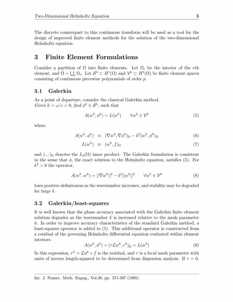
Fig. 1: Two-dimensional bilinear finite element mesh with spacing ∆x = hx and ∆y = hy.
Finite element difference relations are obtained by assembling a patch of four bilin-ear elements as illustrated in Figure 1. The result is the difference stencil associated
Int. J. Numer. Meth. Engng., Vol.38, pp. 371-397 (1995)
Two-Dimensional Helmholtz Equation 8
with the interior node φm,n = φh(mhx, nhy)|R2h 7→ C.
F (k) = Sφm,n − γk2Mφm,n = 0 (22)
where S and M are the two-dimensional linear difference operators emanating fromthe assembled stiffness (discrete Laplacian) and mass tensors respectively.
S =1∑
p,q=−1
spqEpxEqy = Sx + Sy (23)
Sx = −1
h2x(1 +
ε
6δ2y)δ
2x (24)
Sy = −1
h2y(1 +
ε
6δ2x)δ
2y (25)
M =1∑
p,q=−1
mpqEpxEqy =Mx ×My (26)
Mx = (1 +ε
6δ2x) (27)
My = (1 +ε
6δ2y) (28)
Expressions for [spq] and [mpq] are given in the Appendix. The directional shiftoperators are defined by,
Epxφm,n = φm+p,n and Eqyφm,n = φm,n+q (29)
and the central difference operators are defined by,
δ2xφm,n = φm−1,n − 2φm,n + φm+1,n (30)
δ2yφm,n = φm,n−1 − 2φm,n + φm,n+1 (31)
The ε is a general quadrature parameter equal to 1 for exact Gaussian quadratureand 0 for Lobatto quadrature. The mass operatorM is referred to as consistent whenε = 1 and lumped when ε = 0.
Int. J. Numer. Meth. Engng., Vol.38, pp. 371-397 (1995)
Two-Dimensional Helmholtz Equation 9
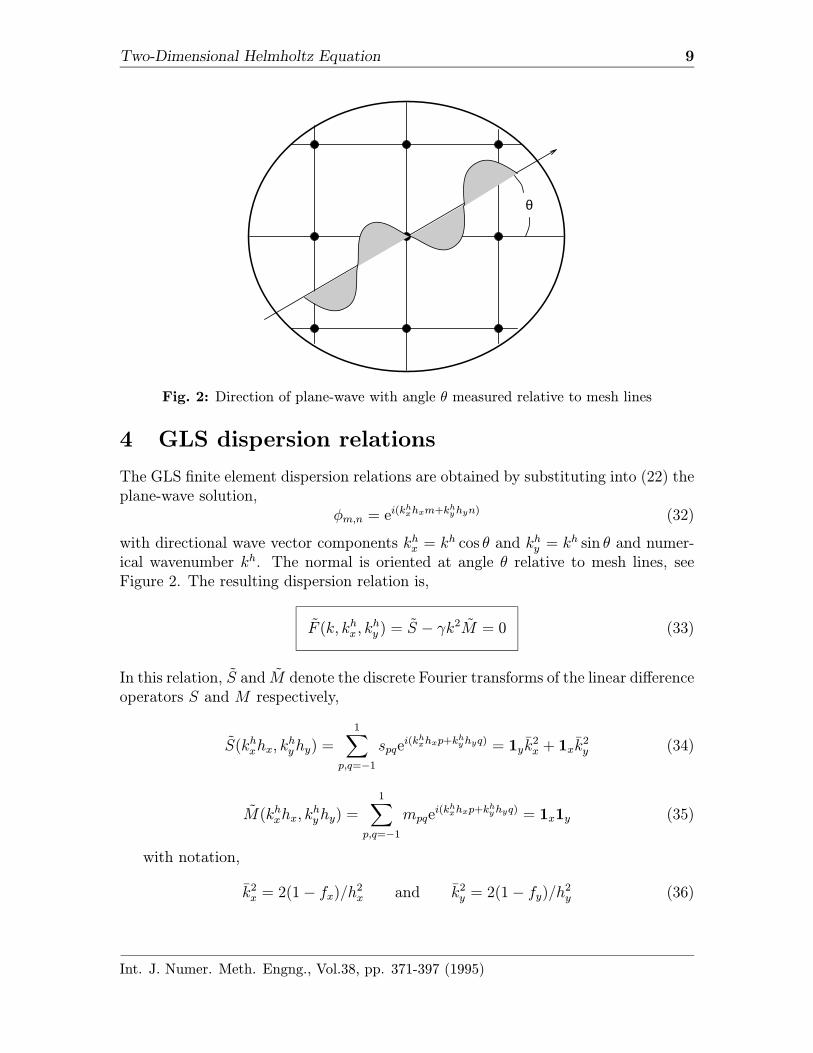
θ
Fig. 2: Direction of plane-wave with angle θ measured relative to mesh lines
4 GLS dispersion relations
The GLS finite element dispersion relations are obtained by substituting into (22) theplane-wave solution,
φm,n = ei(khxhxm+k
hyhyn) (32)
with directional wave vector components khx = kh cos θ and khy = kh sin θ and numer-ical wavenumber kh. The normal is oriented at angle θ relative to mesh lines, seeFigure 2. The resulting dispersion relation is,
F (k, khx , khy ) = S − γk
2M = 0 (33)
In this relation, S and M denote the discrete Fourier transforms of the linear differenceoperators S and M respectively,
S(khxhx, khyhy) =
1∑p,q=−1
spqei(khxhxp+k
hyhyq) = 1yk
2x + 1xk
2y (34)
M(khxhx, khyhy) =
1∑p,q=−1
mpqei(khxhxp+k
hyhyq) = 1x1y (35)
with notation,
k2x = 2(1− fx)/h2x and k2y = 2(1− fy)/h
2y (36)
Int. J. Numer. Meth. Engng., Vol.38, pp. 371-397 (1995)
Two-Dimensional Helmholtz Equation 10
fx = cos(khxhx) = cos(khhx cos θ)
fy = cos(khyhy) = cos(khhy sin θ)
1x = 1−ε
6(kxhx)
2 and 1y = 1−ε
6(kyhy)
2 (37)
For a detailed description of the discrete Fourier transform applied to linear differ-ence equations, see Vichnevetsky and Bowles [24]. The characteristic equation (33)describes the nonlinear relationship between the continuous wavenumber k = ω/cand the finite element discrete wave vector components khx and k
hy . Written in the
alternate form,γk2 = Dh(kh, θ), Dh = S/M (38)
it is clear that the dispersion relation depends on both the magnitude kh and theorientation θ.
kh = |kh| =√(khx)
2 + (khy )2 (39)
θ = tan−1(khy/khx) (40)
5 Optimal GLS mesh parameter for bilinear ele-ments
The optimal least-squares mesh parameter τ is obtained by requiring the phase to beexact, i.e. k = kh for any choice of wave vector angle θ = θo. This requirement ismet by replacing kh with the exact wavenumber, k = ω/c, in the GLS finite elementdispersion relation (38), restricting hx = hy = h, and solving for γ. With this designcriteria, the optimal τ is defined as,
τk2 := 1−S(kh, θo)
k2M(kh, θo)(41)
where S and M are defined in (34) through (37) with kh replaced with k = ω/c. Inparticular, for exact 2× 2 Gaussian integration, the expression for the optimal GLSmesh parameter is,
τk2 = 1−6(4− fx − fy − 2fxfy)
(kh)2(2 + fx)(2 + fy)(42)
Setting θ0 = 0, (41) specializes to,
τk2 := 1−6(1− cos kh)
(kh)2(3− ε(1− cos kh))(43)
which yields exact phase for plane-waves directed along uniform mesh lines. Whenε = 1 this definition specializes to the GLS parameter derived by Harari and Hughes
Int. J. Numer. Meth. Engng., Vol.38, pp. 371-397 (1995)
Two-Dimensional Helmholtz Equation 11
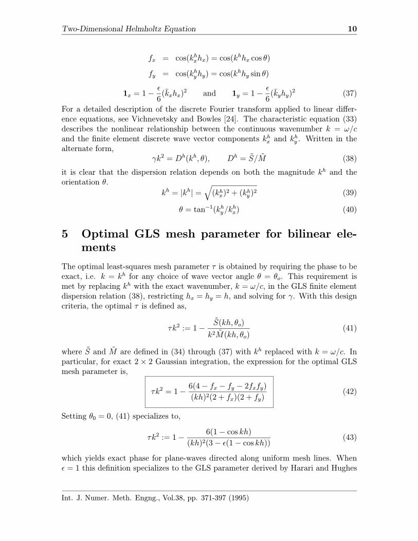
[21] in one-dimension. For comparison the GLS mesh parameter τ defined in (42),with ε = 1, designed to give exact phase for plane-waves oriented along θ = 0 (denotedτ0) and θ = 22.5 (denoted τ22.5) are plotted in Figure 3.
Normalized Wavenumber (kh)=
-0.45
-0.40
-0.35
-0.30
-0.25
-0.20
-0.15
-0.10
-0.05
0
0 0.2 0.4 0.6 0.8
0
22:5
k
2
Fig. 3: Galerkin least squares parameters for two-dimensions designed to give exact phasefor plane waves directed along θ = 0 (denoted τ0), and θ = 22.5 (denoted τ22.5).
In the next section, the performance of alternate GLS mesh parameters, based ondefinition (41), with different choices of θo and ε are examined.
5.1 GLS Dispersion results
The accuracy of the numerical solution is assessed in terms of the phase error definedby,
ep(kh, θ) =
ch
c=
k
kh(44)
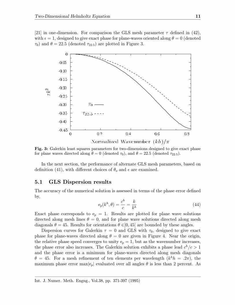
Exact phase corresponds to ep = 1. Results are plotted for plane wave solutionsdirected along mesh lines θ = 0, and for plane wave solutions directed along meshdiagonals θ = 45. Results for orientations θ ∈]0, 45[ are bounded by these angles.Dispersion curves for Galerkin τ = 0 and GLS with τ0, designed to give exact
phase for plane-waves directed along θ = 0 are given in Figure 4. Near the origin,the relative phase speed converges to unity ep = 1, but as the wavenumber increases,the phase error also increases. The Galerkin solution exhibits a phase lead ch/c > 1and the phase error is a minimum for plane-waves directed along mesh diagonalsθ = 45. For a mesh refinement of ten elements per wavelength (khh = .2π), themaximum phase error max|ep| evaluated over all angles θ is less than 2 percent. As
Int. J. Numer. Meth. Engng., Vol.38, pp. 371-397 (1995)
Two-Dimensional Helmholtz Equation 12
Normalized Wavenumber (khh)=
0.96
0.98
1.00
1.02
1.04
1.06
1.08
1.10
0 0.1 0.2 0.3 0.4 0.5
= 0
= 22:5
= 45
Phaseerror(ch=c)
Normalized Wavenumber (khh=)
0.96
0. 98
1. 00
1. 02
1. 04
1. 06
1. 08
1. 10
0 0. 1 0. 2 0. 3 0. 4 0. 5
= 0
= 22 :5
= 45
Phaseerror(ch=c)
Fig. 4: Phase error using exact integration for (top) Galerkin τ = 0, (bottom) GLS τ = τ0,designed to give exact phase for θ = 0.
Int. J. Numer. Meth. Engng., Vol.38, pp. 371-397 (1995)
Two-Dimensional Helmholtz Equation 13
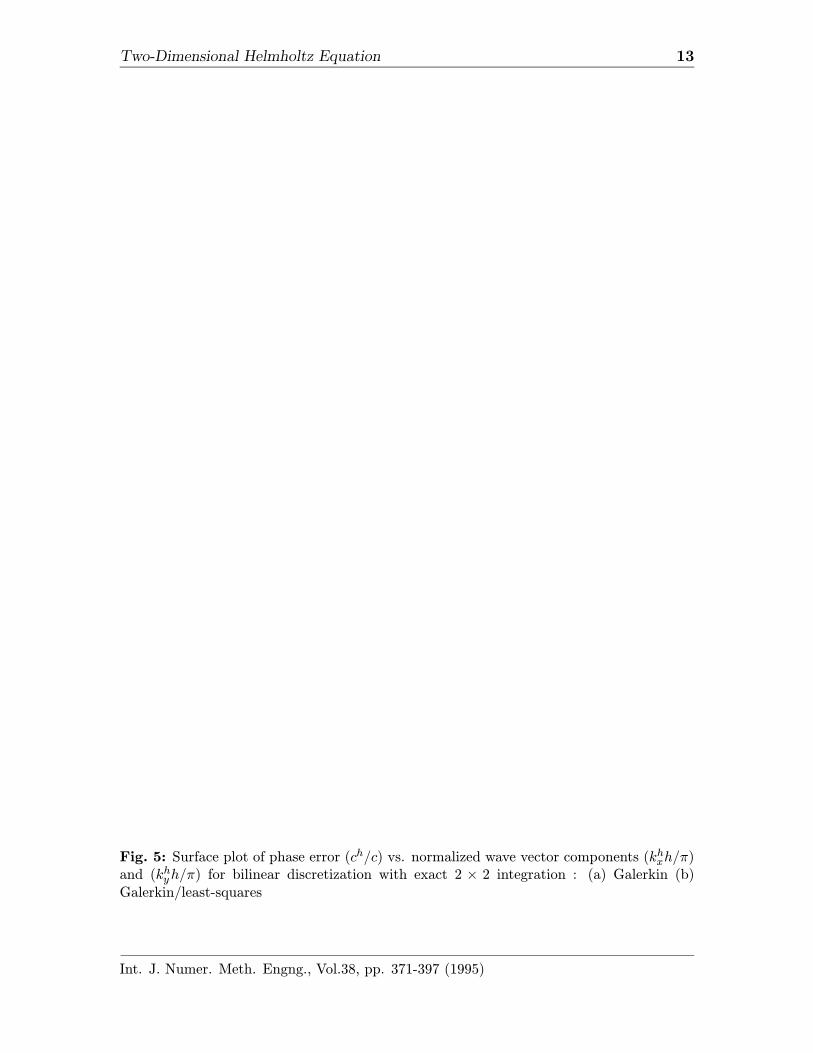
Fig. 5: Surface plot of phase error (ch/c) vs. normalized wave vector components (khxh/π)and (khyh/π) for bilinear discretization with exact 2 × 2 integration : (a) Galerkin (b)Galerkin/least-squares
Int. J. Numer. Meth. Engng., Vol.38, pp. 371-397 (1995)
Two-Dimensional Helmholtz Equation 14
Normalized Wavenumber (khh=)
0.96
0.98
1.00
1.02
1.04
1.06
1.08
1.10
0 0.1 0.2 0.3 0.4 0.5
= 0
= 22:5
= 45
Phaseerror(ch=c)
Normalized Wavenumber (khh=)
0.96
0. 98
1. 00
1. 02
1. 04
1. 06
1. 08
1. 10
0 0. 1 0. 2 0. 3 0. 4 0. 5
= 0
= 22 :5
= 45
Phaseerror(ch=c)
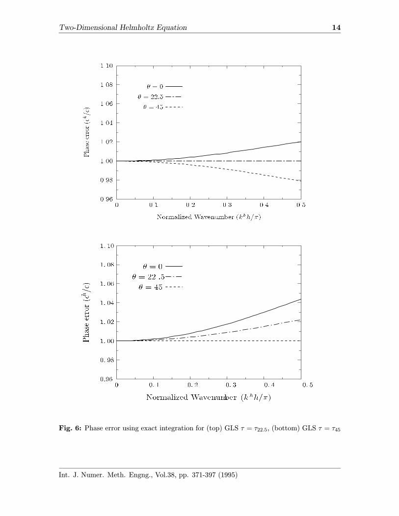
Fig. 6: Phase error using exact integration for (top) GLS τ = τ22.5, (bottom) GLS τ = τ45
Int. J. Numer. Meth. Engng., Vol.38, pp. 371-397 (1995)

Two-Dimensional Helmholtz Equation 15
-1.0
-0.5
0
0.5
1.0
1.5
2.0
0 10 20 30 40 50
Galerkin
22:5
0
ep
percenterror
-4
-2
0
2
4
6
8
10
12
0 10 20 30 40 50
Galerkin
22:5
0
ep
percenterror
Fig. 7: Phase error using exact integration at (top) 10 elements per wavelength, (bottom)4 elements per wavelength.
Int. J. Numer. Meth. Engng., Vol.38, pp. 371-397 (1995)
Two-Dimensional Helmholtz Equation 16
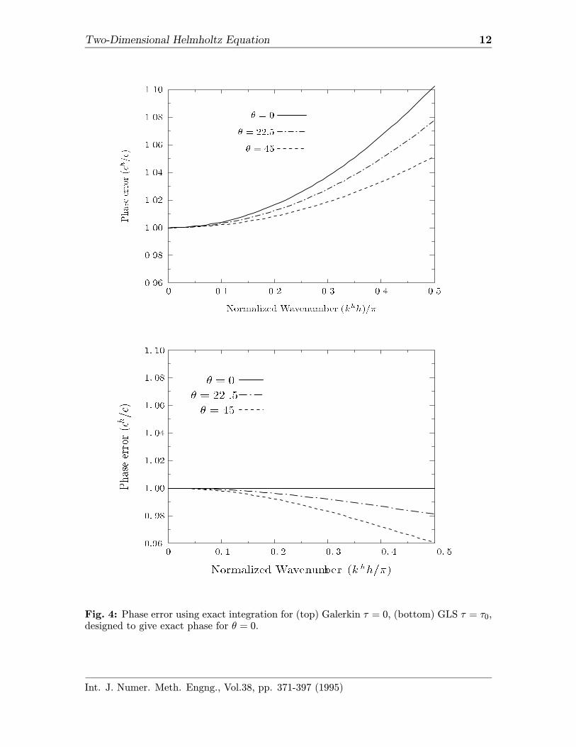
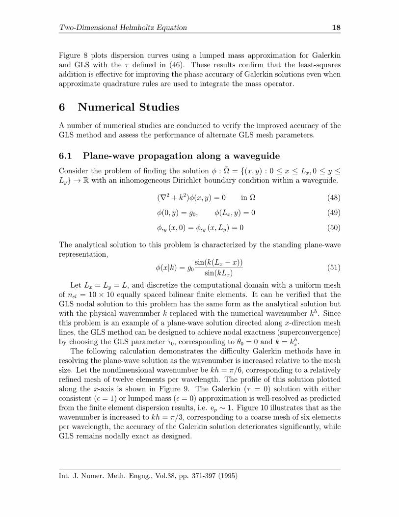
the wavenumber is increased relative to the mesh parameter h, the phase accuracydegrades severely to max|ep| = 10 percent. For GLS with τ0 and exact integration,the two-dimensional GLS dispersion relation relating the exact wavenumber k = ω/c,to the discrete wavenumber kh and angle θ is given by,
kh = cos−14(fx + fy) + 5fxfy − 4
fx + fy − fxfy + 8
(45)
By design, for propagation along mesh lines θ = 0 (mod 90), this relation reducesto the exact phase relationship ep = 1 for kh ∈ (0, π). Referring to Figure 4, thedispersion curves for θ 6= 0 exhibit a phase lag ch/c < 1 with max|ep| reduced toapproximately 4 percent at four elements per wavelength. These two-dimensionaldispersion results show how the addition of the least-squares operator, with the GLSmesh parameter τ0 defined in (43), reduces the phase error present in the Galerkinsolution over all wave vector orientations θ. This conclusion is further illustrated inFigure 5 by an elevated surface of the phase error ch/c = k/kh plotted as a functionof the normalized wavenumber components khxh/π in the x-direction and k
hyh/π in
the y–direction .In Figure 6, the dispersion curves for the alternative GLS parameters, τ22.5 de-
signed for exact phase at θ = 22.5, and τ45 designed for exact phase at θ = 45 arecompared. For τ45, the maximum phase error is still approximately 4 percent butis now reflected about the exact solution ch/c = 1 such that there is a phase leadch/c > 1. By choosing the GLS parameter τ22.5, corresponding to exact phase forθ = 22.5, the envelope of the dispersion curves is centered around the exact resultch/c = 1. As a result, the GLS solution exhibits a maximum possible error |ep| of only2 percent at four elements per wavelength as compared to 10 percent for Galerkin.At ten elements per wavelength, GLS with τ22.5 has a maximum possible error of 0.5percent, compared to 1.6 percent for Galerkin. See Figure 7 for a summary of theseresults.In conclusion, firstly, it is clear that the least-squares addition with τ defined by
(41) substantially improves the phase accuracy of the finite element solution for anychoice of wave vector orientation θ. Secondly, we find that when the direction ofwave-propagation is not known a priori, or when it is varying over the mesh, as willgenerally be the case, then τ22.5 is optimal.The effectiveness of the Galerkin/least-squares method when using a lumped mass
approximation (Lobotto quadrature) is examined by setting ε = 0 in (43).
τk2 = 1−2(1− cos kh)
(kh)2(46)
The two-dimensional GLS dispersion relation in this case is,
kh = cos−1 (fx + fy + 2fxfy − 1)/3 (47)
Int. J. Numer. Meth. Engng., Vol.38, pp. 371-397 (1995)
Two-Dimensional Helmholtz Equation 17
Normalized Wavenumber (khh=)
0.84
0. 86
0. 88
0. 90
0. 92
0. 94
0. 96
0. 98
1. 00
1. 02
0 0. 1 0. 2 0. 3 0. 4 0. 5
= 0
= 22 :5
= 45
Phaseerror(ch=c)
Normalized Wavenumber (khh=)
0.84
0. 86
0. 88
0. 90
0. 92
0. 94
0. 96
0. 98
1. 00
1. 02
0 0. 1 0. 2 0. 3 0. 4 0. 5
= 0
= 22 :5
= 45
Phaseerror(ch=c)
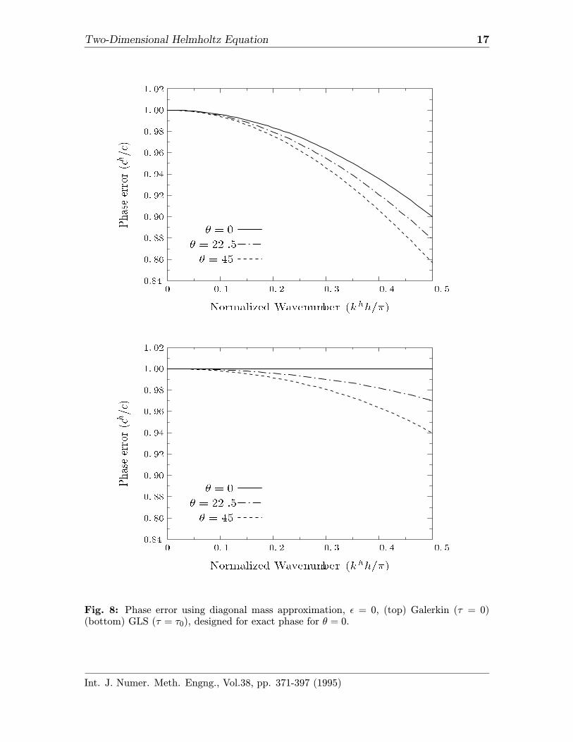
Fig. 8: Phase error using diagonal mass approximation, ε = 0, (top) Galerkin (τ = 0)(bottom) GLS (τ = τ0), designed for exact phase for θ = 0.
Int. J. Numer. Meth. Engng., Vol.38, pp. 371-397 (1995)
Two-Dimensional Helmholtz Equation 18
Figure 8 plots dispersion curves using a lumped mass approximation for Galerkinand GLS with the τ defined in (46). These results confirm that the least-squaresaddition is effective for improving the phase accuracy of Galerkin solutions even whenapproximate quadrature rules are used to integrate the mass operator.
6 Numerical Studies
A number of numerical studies are conducted to verify the improved accuracy of theGLS method and assess the performance of alternate GLS mesh parameters.
6.1 Plane-wave propagation along a waveguide
Consider the problem of finding the solution φ : Ω = (x, y) : 0 ≤ x ≤ Lx, 0 ≤ y ≤Ly → R with an inhomogeneous Dirichlet boundary condition within a waveguide.
(∇2 + k2)φ(x, y) = 0 in Ω (48)
φ(0, y) = g0, φ(Lx, y) = 0 (49)
φ,y (x, 0) = φ,y (x, Ly) = 0 (50)
The analytical solution to this problem is characterized by the standing plane-waverepresentation,
φ(x|k) = g0sin(k(Lx − x))
sin(kLx)(51)
Let Lx = Ly = L, and discretize the computational domain with a uniform meshof nel = 10 × 10 equally spaced bilinear finite elements. It can be verified that theGLS nodal solution to this problem has the same form as the analytical solution butwith the physical wavenumber k replaced with the numerical wavenumber kh. Sincethis problem is an example of a plane-wave solution directed along x-direction meshlines, the GLS method can be designed to achieve nodal exactness (superconvergence)by choosing the GLS parameter τ0, corresponding to θ0 = 0 and k = k
hx .
The following calculation demonstrates the difficulty Galerkin methods have inresolving the plane-wave solution as the wavenumber is increased relative to the meshsize. Let the nondimensional wavenumber be kh = π/6, corresponding to a relativelyrefined mesh of twelve elements per wavelength. The profile of this solution plottedalong the x-axis is shown in Figure 9. The Galerkin (τ = 0) solution with eitherconsistent (ε = 1) or lumped mass (ε = 0) approximation is well-resolved as predictedfrom the finite element dispersion results, i.e. ep ∼ 1. Figure 10 illustrates that as thewavenumber is increased to kh = π/3, corresponding to a coarse mesh of six elementsper wavelength, the accuracy of the Galerkin solution deteriorates significantly, whileGLS remains nodally exact as designed.
Int. J. Numer. Meth. Engng., Vol.38, pp. 371-397 (1995)
Two-Dimensional Helmholtz Equation 19
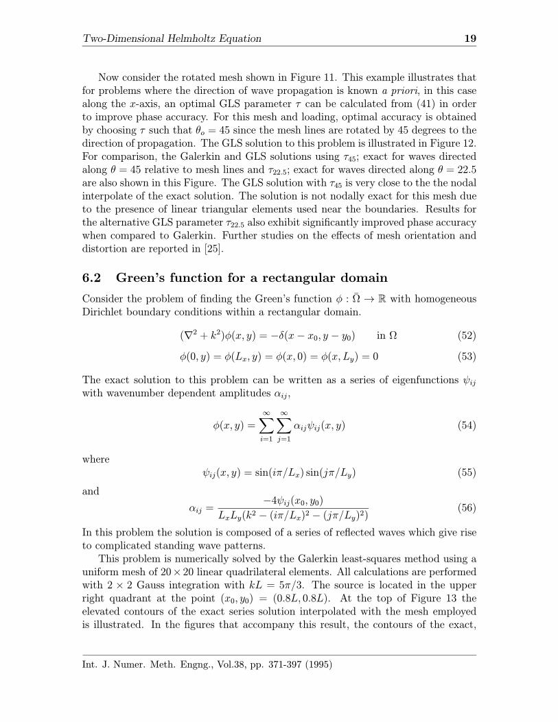
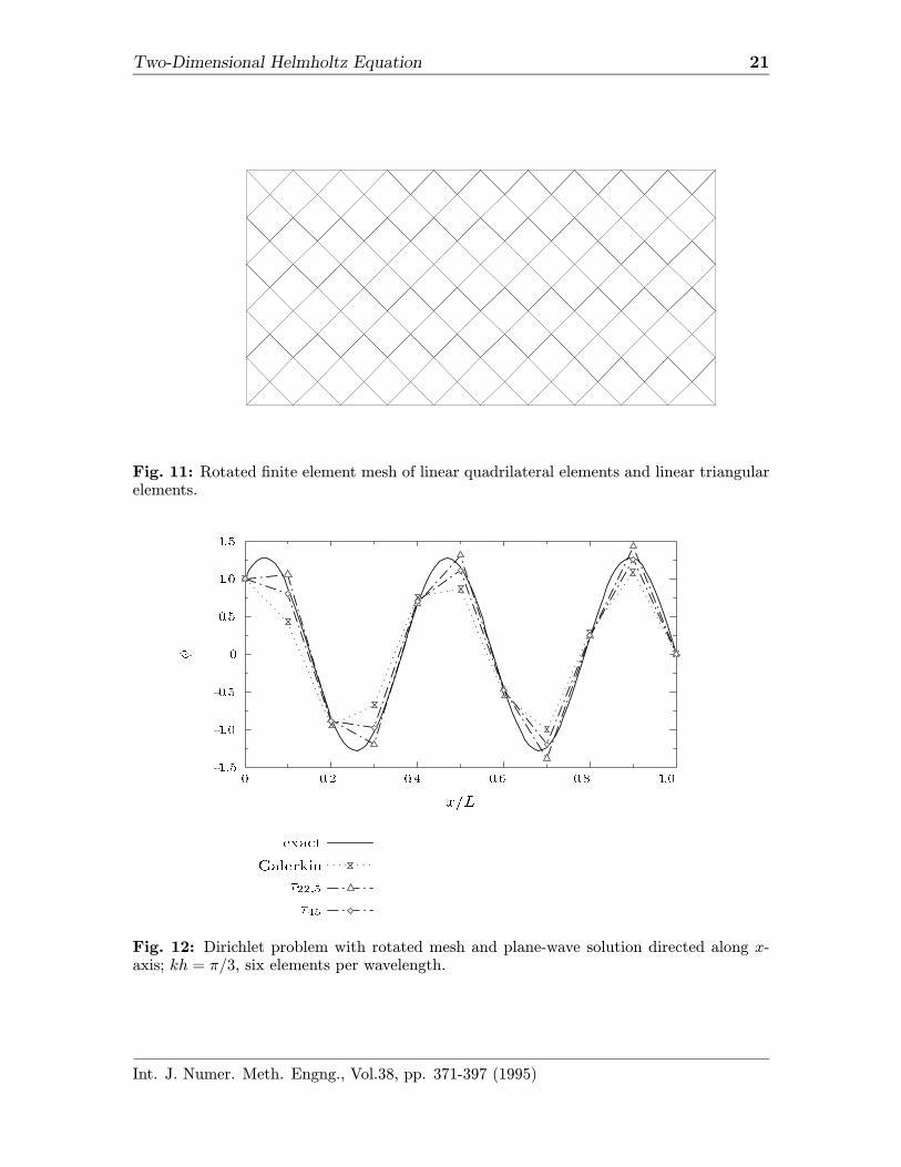
Now consider the rotated mesh shown in Figure 11. This example illustrates thatfor problems where the direction of wave propagation is known a priori, in this casealong the x-axis, an optimal GLS parameter τ can be calculated from (41) in orderto improve phase accuracy. For this mesh and loading, optimal accuracy is obtainedby choosing τ such that θo = 45 since the mesh lines are rotated by 45 degrees to thedirection of propagation. The GLS solution to this problem is illustrated in Figure 12.For comparison, the Galerkin and GLS solutions using τ45; exact for waves directedalong θ = 45 relative to mesh lines and τ22.5; exact for waves directed along θ = 22.5are also shown in this Figure. The GLS solution with τ45 is very close to the the nodalinterpolate of the exact solution. The solution is not nodally exact for this mesh dueto the presence of linear triangular elements used near the boundaries. Results forthe alternative GLS parameter τ22.5 also exhibit significantly improved phase accuracywhen compared to Galerkin. Further studies on the effects of mesh orientation anddistortion are reported in [25].
6.2 Green’s function for a rectangular domain
Consider the problem of finding the Green’s function φ : Ω → R with homogeneousDirichlet boundary conditions within a rectangular domain.
(∇2 + k2)φ(x, y) = −δ(x− x0, y − y0) in Ω (52)
φ(0, y) = φ(Lx, y) = φ(x, 0) = φ(x, Ly) = 0 (53)
The exact solution to this problem can be written as a series of eigenfunctions ψijwith wavenumber dependent amplitudes αij,
φ(x, y) =∞∑i=1
∞∑j=1
αijψij(x, y) (54)
whereψij(x, y) = sin(iπ/Lx) sin(jπ/Ly) (55)
and
αij =−4ψij(x0, y0)
LxLy(k2 − (iπ/Lx)2 − (jπ/Ly)2)(56)
In this problem the solution is composed of a series of reflected waves which give riseto complicated standing wave patterns.This problem is numerically solved by the Galerkin least-squares method using a
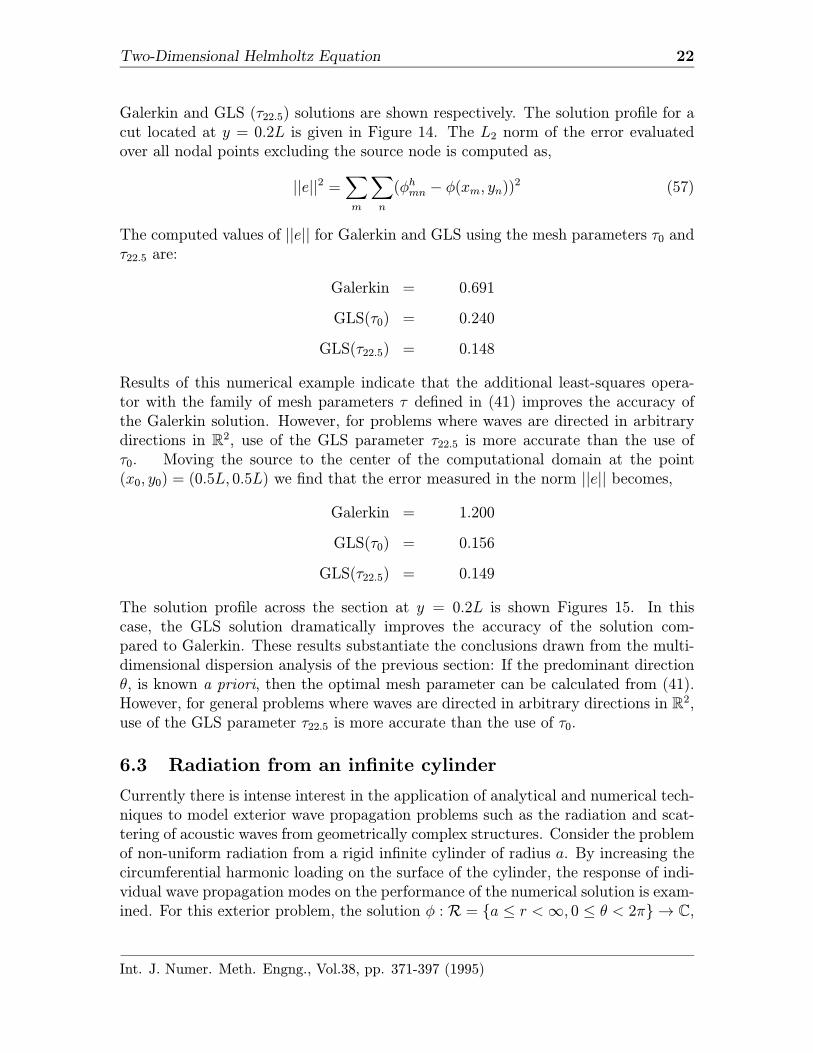
uniform mesh of 20×20 linear quadrilateral elements. All calculations are performedwith 2 × 2 Gauss integration with kL = 5π/3. The source is located in the upperright quadrant at the point (x0, y0) = (0.8L, 0.8L). At the top of Figure 13 theelevated contours of the exact series solution interpolated with the mesh employedis illustrated. In the figures that accompany this result, the contours of the exact,
Int. J. Numer. Meth. Engng., Vol.38, pp. 371-397 (1995)
Two-Dimensional Helmholtz Equation 20
x=L
-1.5
-1.0
-0.5
0
0.5
1.0
1.5
0 0.2 0.4 0.6 0.8 1.0
exact
Galerkin = 1
Gal erki n =0
GLS
Fig. 9: Dirichlet problem with plane-wave solution directed along x-direction mesh lineswith kh = π/6, twelve elements per wavelength.
x=L
-2.0
-1.5
-1.0
-0.5
0
0.5
1.0
1.5
2.0
0 0.2 0.4 0.6 0.8 1.0
exact
Galerkin = 1
Gal erki n =0
GLS
Fig. 10: Dirichlet problem with plane-wave solution directed along x-direction mesh lineswith kh = π/3, six elements per wavelength.
Int. J. Numer. Meth. Engng., Vol.38, pp. 371-397 (1995)
Two-Dimensional Helmholtz Equation 21
Fig. 11: Rotated finite element mesh of linear quadrilateral elements and linear triangularelements.
x=L
-1.5
-1.0
-0.5
0
0.5
1.0
1.5
0 0.2 0.4 0.6 0.8 1.0
exact
Galerkin
22:5
45
Fig. 12: Dirichlet problem with rotated mesh and plane-wave solution directed along x-axis; kh = π/3, six elements per wavelength.
Int. J. Numer. Meth. Engng., Vol.38, pp. 371-397 (1995)
Two-Dimensional Helmholtz Equation 22
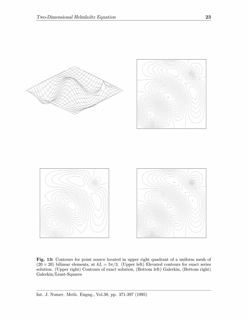
Galerkin and GLS (τ22.5) solutions are shown respectively. The solution profile for acut located at y = 0.2L is given in Figure 14. The L2 norm of the error evaluatedover all nodal points excluding the source node is computed as,
||e||2 =∑m
∑n
(φhmn − φ(xm, yn))2 (57)
The computed values of ||e|| for Galerkin and GLS using the mesh parameters τ0 andτ22.5 are:
Galerkin = 0.691
GLS(τ0) = 0.240
GLS(τ22.5) = 0.148
Results of this numerical example indicate that the additional least-squares opera-tor with the family of mesh parameters τ defined in (41) improves the accuracy ofthe Galerkin solution. However, for problems where waves are directed in arbitrarydirections in R2, use of the GLS parameter τ22.5 is more accurate than the use ofτ0. Moving the source to the center of the computational domain at the point(x0, y0) = (0.5L, 0.5L) we find that the error measured in the norm ||e|| becomes,
Galerkin = 1.200
GLS(τ0) = 0.156
GLS(τ22.5) = 0.149
The solution profile across the section at y = 0.2L is shown Figures 15. In thiscase, the GLS solution dramatically improves the accuracy of the solution com-pared to Galerkin. These results substantiate the conclusions drawn from the multi-dimensional dispersion analysis of the previous section: If the predominant directionθ, is known a priori, then the optimal mesh parameter can be calculated from (41).However, for general problems where waves are directed in arbitrary directions in R2,use of the GLS parameter τ22.5 is more accurate than the use of τ0.
6.3 Radiation from an infinite cylinder
Currently there is intense interest in the application of analytical and numerical tech-niques to model exterior wave propagation problems such as the radiation and scat-tering of acoustic waves from geometrically complex structures. Consider the problemof non-uniform radiation from a rigid infinite cylinder of radius a. By increasing thecircumferential harmonic loading on the surface of the cylinder, the response of indi-vidual wave propagation modes on the performance of the numerical solution is exam-ined. For this exterior problem, the solution φ : R = a ≤ r <∞, 0 ≤ θ < 2π → C,
Int. J. Numer. Meth. Engng., Vol.38, pp. 371-397 (1995)
Two-Dimensional Helmholtz Equation 23
Fig. 13: Contours for point source located in upper right quadrant of a uniform mesh of(20 × 20) bilinear elements, at kL = 5π/3. (Upper left) Elevated contours for exact seriessolution. (Upper right) Contours of exact solution, (Bottom left) Galerkin, (Bottom right)Galerkin/Least-Squares
Int. J. Numer. Meth. Engng., Vol.38, pp. 371-397 (1995)
Two-Dimensional Helmholtz Equation 24
x=L
-0.6
-0.5
-0.4
-0.3
-0.2
-0.1
0
0.1
0 0.2 0.4 0.6 0.8 1.0
series
Galerki n
0
22:5
Fig. 14: Point source located in upper right quadrant: Solution profile along x–axis forfixed y/L = 0.2
x=L
0
0.1
0. 2
0. 3
0. 4
0. 5
0. 6
0 0. 2 0. 4 0. 6 0. 8 1. 0
series
Galerki n
0
22:5
Fig. 15: Point source located at center of square domain: Solution profile along x–axis forfixed y/L = 0.2
Int. J. Numer. Meth. Engng., Vol.38, pp. 371-397 (1995)
Two-Dimensional Helmholtz Equation 25
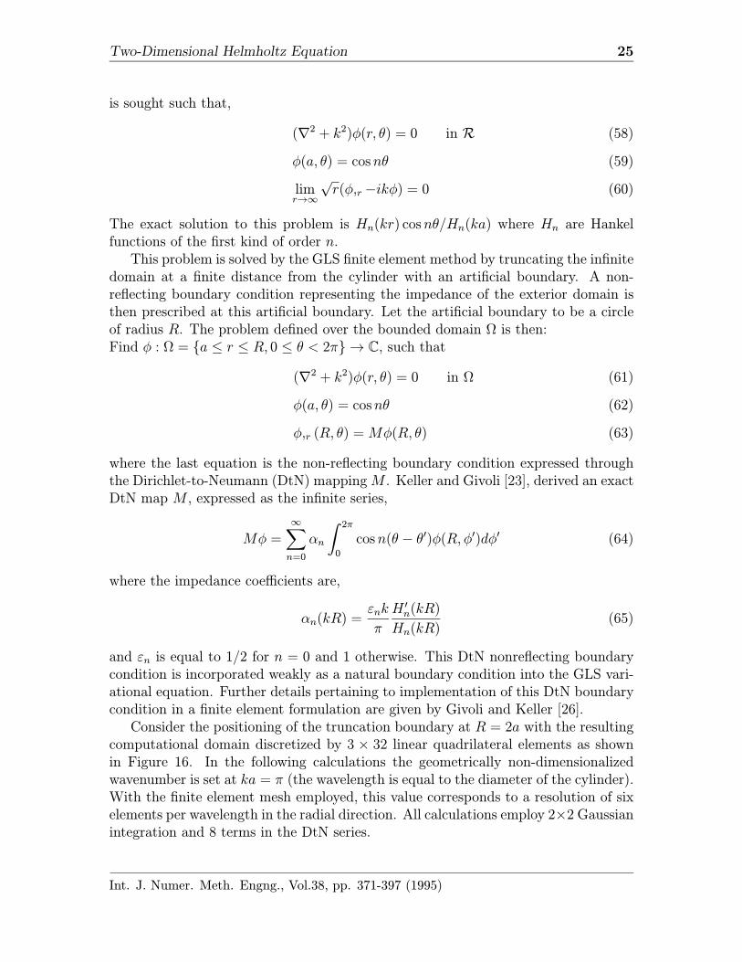
is sought such that,
(∇2 + k2)φ(r, θ) = 0 in R (58)
φ(a, θ) = cosnθ (59)
limr→∞
√r(φ,r−ikφ) = 0 (60)
The exact solution to this problem is Hn(kr) cosnθ/Hn(ka) where Hn are Hankelfunctions of the first kind of order n.This problem is solved by the GLS finite element method by truncating the infinite
domain at a finite distance from the cylinder with an artificial boundary. A non-reflecting boundary condition representing the impedance of the exterior domain isthen prescribed at this artificial boundary. Let the artificial boundary to be a circleof radius R. The problem defined over the bounded domain Ω is then:Find φ : Ω = a ≤ r ≤ R, 0 ≤ θ < 2π → C, such that
(∇2 + k2)φ(r, θ) = 0 in Ω (61)
φ(a, θ) = cosnθ (62)
φ,r (R, θ) =Mφ(R, θ) (63)
where the last equation is the non-reflecting boundary condition expressed throughthe Dirichlet-to-Neumann (DtN) mappingM . Keller and Givoli [23], derived an exactDtN map M , expressed as the infinite series,
Mφ =∞∑n=0
αn
∫ 2π0
cosn(θ − θ′)φ(R, φ′)dφ′ (64)
where the impedance coefficients are,
αn(kR) =εnk
π
H ′n(kR)
Hn(kR)(65)
and εn is equal to 1/2 for n = 0 and 1 otherwise. This DtN nonreflecting boundarycondition is incorporated weakly as a natural boundary condition into the GLS vari-ational equation. Further details pertaining to implementation of this DtN boundarycondition in a finite element formulation are given by Givoli and Keller [26].Consider the positioning of the truncation boundary at R = 2a with the resulting
computational domain discretized by 3 × 32 linear quadrilateral elements as shownin Figure 16. In the following calculations the geometrically non-dimensionalizedwavenumber is set at ka = π (the wavelength is equal to the diameter of the cylinder).With the finite element mesh employed, this value corresponds to a resolution of sixelements per wavelength in the radial direction. All calculations employ 2×2 Gaussianintegration and 8 terms in the DtN series.
Int. J. Numer. Meth. Engng., Vol.38, pp. 371-397 (1995)
Two-Dimensional Helmholtz Equation 26
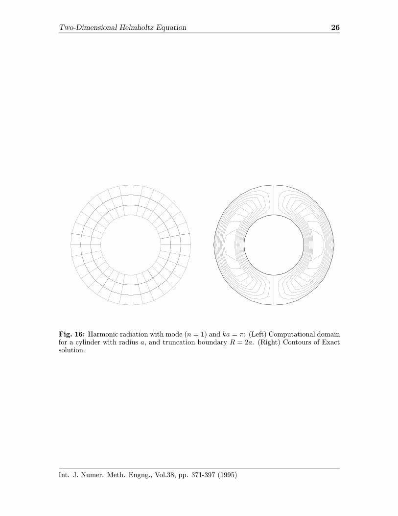
Fig. 16: Harmonic radiation with mode (n = 1) and ka = π: (Left) Computational domainfor a cylinder with radius a, and truncation boundary R = 2a. (Right) Contours of Exactsolution.
Int. J. Numer. Meth. Engng., Vol.38, pp. 371-397 (1995)
Two-Dimensional Helmholtz Equation 27
For the first harmonic n = 0, the exact solution is a simple cylindrical wave whichhas the character of a radially decaying plane-wave. For the radially uniform meshemployed, this problem reduces to a one dimensional problem with radial coordinater. Taking h to be the element length in the r-direction, Harari and Hughes [22] haveshown that the GLS parameter τ0 is optimal in this case.In this paper, the higher-order circumferential harmonics n = 1 through n = 4 are
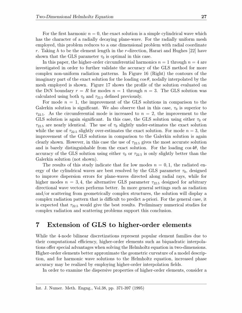
investigated in order to further validate the accuracy of the GLS method for morecomplex non-uniform radiation patterns. In Figure 16 (Right) the contours of theimaginary part of the exact solution for the loading cos θ, nodally interpolated by themesh employed is shown. Figure 17 shows the profile of the solution evaluated onthe DtN boundary r = R for modes n = 1 through n = 3. The GLS solution wascalculated using both τ0 and τ22.5 defined previously.For mode n = 1, the improvement of the GLS solutions in comparison to the
Galerkin solution is significant. We also observe that in this case, τ0 is superior toτ22.5. As the circumferential mode is increased to n = 2, the improvement to theGLS solution is again significant. In this case, the GLS solution using either τ0 orτ22.5 are nearly identical. The use of τ0 slightly under-estimates the exact solutionwhile the use of τ22.5 slightly over-estimates the exact solution. For mode n = 3, theimprovement of the GLS solutions in comparison to the Galerkin solution is againclearly shown. However, in this case the use of τ22.5 gives the most accurate solutionand is barely distinguishable from the exact solution. For the loading cos 4θ, theaccuracy of the GLS solution using either τ0 or τ22.5 is only slightly better than theGalerkin solution (not shown).The results of this study indicate that for low modes n = 0, 1, the radiated en-
ergy of the cylindrical waves are best resolved by the GLS parameter τ0, designedto improve dispersion errors for plane-waves directed along radial rays, while forhigher modes n = 3, 4, the alternative GLS parameter τ22.5 designed for arbitrarydirectional wave vectors performs better. In more general settings such as radiationand/or scattering from geometrically complex structures, the solution will display acomplex radiation pattern that is difficult to predict a-priori. For the general case, itis expected that τ22.5 would give the best results. Preliminary numerical studies forcomplex radiation and scattering problems support this conclusion.
7 Extension of GLS to higher-order elements
While the 4-node bilinear discretizations represent popular element families due totheir computational efficiency, higher-order elements such as biquadratic interpola-tions offer special advantages when solving the Helmholtz equation in two-dimensions.Higher-order elements better approximate the geometric curvature of a model descrip-tion, and for harmonic wave solutions to the Helmholtz equation, increased phaseaccuracy may be realized by employing higher-order interpolation fields.In order to examine the dispersive properties of higher-order elements, consider a
Int. J. Numer. Meth. Engng., Vol.38, pp. 371-397 (1995)
Two-Dimensional Helmholtz Equation 28
=
-0.20
- 0. 15
- 0. 10
- 0. 05
0
0. 05
0. 10
0. 15
0. 20
0 0. 2 0. 4 0. 6 0. 8 1. 0
exact
Galerkin
0
22:5
Im
=
-0.3
-0.2
-0.1
0
0.1
0.2
0.3
0 0.2 0.4 0.6 0.8 1.0
exact
Galerkin
0
22:5
Im
=
-0.5
-0.4
-0.3
-0.2
-0.1
0
0.1
0.2
0.3
0.4
0.5
0 0.2 0.4 0.6 0.8 1.0
exact
Galerkin
0
22:5
Im
Fig. 17: Harmonic radiation from a cylinder with ka = π. Solution plotted along thetruncation boundary R = 2a. From top to bottom, mode n = 1 , 2 , 3
Int. J. Numer. Meth. Engng., Vol.38, pp. 371-397 (1995)
Two-Dimensional Helmholtz Equation 29
(m,n)
(m-2,n+2)
(m-2,n-2)
(m,n+2)
(m,n-2) (m+2,n-2)
(m+2,n)
(m+2,n+2)
(m-2,n)
Fig. 18: Two-dimensional biquadratic finite element mesh with corner, edge, and internalnodes.
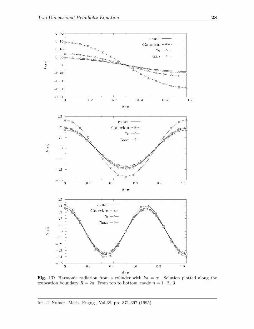
uniform mesh of biquadratic (P2 × P2) elements with length h = 2∆x = 2∆y. Forsimplicity, consider the Galerkin method where τ = 0. By assembling a patch of 4elements as shown in Figure 18, we identify four different difference stencils, eachhaving the form,
∑p,q
(spq −(kh)2
10mpq)E
pxEqyφm,n = 0 (66)
These four stencils are associated with the following nodes where the range on thesum (p, q) is indicated.
(φm,n) corner nodes (p, q) ∈ −2, 2 × −2, 2(φm+1,n) x-direction edge nodes (p, q) ∈ 0, 2 × −2, 2(φm,n+1) y-direction edge nodes (p, q) ∈ −2, 2 × 0, 2(φm+1,n+1) interior nodes (p, q) ∈ 0, 2 × 0, 2
Expressions for the difference coefficients [spq] and [mpq] are given in the Appendix.In this case, the numerical solutions are allowed to assume four different amplitudes
Int. J. Numer. Meth. Engng., Vol.38, pp. 371-397 (1995)
Two-Dimensional Helmholtz Equation 30
corresponding to each of the four different stencils,
φm,n = A1µmx µny
φm+1,n = A2µm+1x µny
φm,n+1 = A3µmx µn+1y
φm+1,n+1 = A4µm+1x µn+1y
(67)
whereµx = e
ikhx∆x and µy = eikhy∆y (68)
The constants A1 and A4 represent amplitudes at the corner and the interior nodesof the element, while A2 and A3 denote the amplitudes at the edges parallel to the xand y axis respectively. Substituting the above discrete solutions into each recurrencestencil yields the characteristic matrix equations,
[S −(kh)2
10M ]A = 0 (69)
where S and M are symmetric (4 × 4) characteristic matrices depending on (khxh)and (khyh), and A ∈ R
4 is the column of amplitudes. The characteristic functions
[Sij] and [Mij] are given in the Appendix.The dispersion relation is obtained by setting the determinant of this characteris-
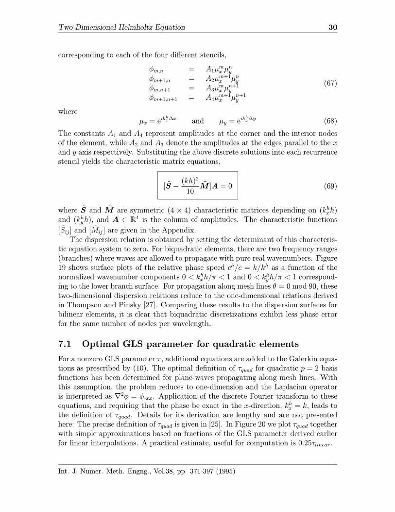
tic equation system to zero. For biquadratic elements, there are two frequency ranges(branches) where waves are allowed to propagate with pure real wavenumbers. Figure19 shows surface plots of the relative phase speed ch/c = k/kh as a function of thenormalized wavenumber components 0 < khxh/π < 1 and 0 < khyh/π < 1 correspond-ing to the lower branch surface. For propagation along mesh lines θ = 0 mod 90, thesetwo-dimensional dispersion relations reduce to the one-dimensional relations derivedin Thompson and Pinsky [27]. Comparing these results to the dispersion surfaces forbilinear elements, it is clear that biquadratic discretizations exhibit less phase errorfor the same number of nodes per wavelength.
7.1 Optimal GLS parameter for quadratic elements
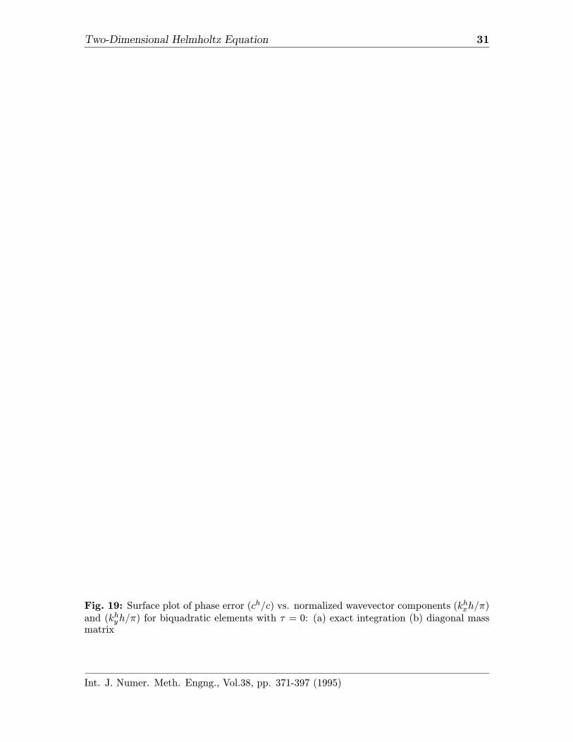
For a nonzero GLS parameter τ , additional equations are added to the Galerkin equa-tions as prescribed by (10). The optimal definition of τquad for quadratic p = 2 basisfunctions has been determined for plane-waves propagating along mesh lines. Withthis assumption, the problem reduces to one-dimension and the Laplacian operatoris interpreted as ∇2φ = φ,xx. Application of the discrete Fourier transform to theseequations, and requiring that the phase be exact in the x-direction, khx = k, leads tothe definition of τquad. Details for its derivation are lengthy and are not presentedhere: The precise definition of τquad is given in [25]. In Figure 20 we plot τquad togetherwith simple approximations based on fractions of the GLS parameter derived earlierfor linear interpolations. A practical estimate, useful for computation is 0.25τlinear.
Int. J. Numer. Meth. Engng., Vol.38, pp. 371-397 (1995)
Two-Dimensional Helmholtz Equation 31
Fig. 19: Surface plot of phase error (ch/c) vs. normalized wavevector components (khxh/π)and (khyh/π) for biquadratic elements with τ = 0: (a) exact integration (b) diagonal massmatrix
Int. J. Numer. Meth. Engng., Vol.38, pp. 371-397 (1995)
Two-Dimensional Helmholtz Equation 32
kh=
-0.25
-0.20
-0.15
-0.10
-0.05
0
0 0.3 0.6 0.9
quad
1
2linear
1
4l i near
k2
Fig. 20: Galerkin/least-squares weighting parameter τquad for quadratic interpolation usingGaussian quadrature compared to estimates based on fractions of the linear τlinear.
Int. J. Numer. Meth. Engng., Vol.38, pp. 371-397 (1995)
Two-Dimensional Helmholtz Equation 33
8 Conclusions
In this paper we have presented a Galerkin/least-squares (GLS) finite element methodfor two-dimensional wave propagation governed by the Helmholtz equation. The GLSparameter τ is designed from the criterion that numerical phase error be reduced inthe primary direction of wave propagation. Results from a two-dimensional discreteFourier analysis of the GLS method indicate that the additional least-squares opera-tor improves the accuracy of the Galerkin solution over all wave vector orientations.Accurate GLS solutions are maintained for as little as six linear elements per wave-length compared to the limit of ten elements per wavelength required for well resolvedGalerkin solutions.A number of alternative GLS parameters were derived for general numerical inte-
gration rules such as Gaussian and Lobatto quadrature. Results from the dispersionanalysis indicate that phase accuracy and directional properties associated with GLSusing either exact integration, or diagonal mass approximations, are significantly im-proved when compared to Galerkin.Numerical examples of plane waves traveling along a two-dimensional waveguide
with uniform and rotated mesh orientations verify that as the wavenumber, normal-ized with respect to the element size, is increased, the degradation in phase accuracypresent in the Galerkin solution is reduced and in some cases eliminated by the properchoice of the GLS parameter τ . GLS solutions for the Green’s function in the interiorof simple rectangular domains demonstrates the improved performance compared tothe standard Galerkin method where multiple reflections are present. These resultsvalidate our conclusion that for problems where waves are directed in arbitrary direc-tions, use of the GLS parameter τ22.5 defined in (41) with θo = 22.5, is more accuratethan the use of τ0, designed to give exact phase for one-dimensional solutions.By increasing the circumferential harmonics for a radiating cylindrical model, the
response of individual modes on the performance of the numerical solutions has beeninvestigated. Results indicate that for low modes, the radiated energy of the cylindri-cal waves are best resolved by the GLS parameter τ0, designed to improve dispersionerrors for plane-waves directed along the radial rays, while for higher modes, the al-ternate GLS parameter τ22.5, designed for arbitrary directional wave vectors performsoptimally.The extension of the GLS method for the Helmholtz equation to higher-order
interpolations has also been investigated. Optimal GLS parameters for elements withbasis functions of high spectral order p can be approximated by simple fractionsof the first order p = 1 case. In particular, for quadratic elements (p = 2), thevalue τ = .25τlinear proves to be a useful estimate. Optimal GLS parameters forthe Helmholtz equation in R3 have also been determined: Results are reported inThompson and Pinsky [28] and Thompson [25].
Int. J. Numer. Meth. Engng., Vol.38, pp. 371-397 (1995)
Two-Dimensional Helmholtz Equation 34
Acknowledgments
This research was supported by ONR under contracts N00014-89-J-1951 and N00014-92-J-1774. The first author was also supported in part by an Achievement Rewards forCollege Scientists (ARCS) scholarship. This support is gratefully acknowledged. Theauthors would also like to thank Isaac Harari and Thomas J.R. Hughes for introducingus to Galerkin/least-squares technology and its many attributes, and Raja Jasti foruseful discussions on biquadratic dispersion analysis.
References
[1] Bayliss,A.; Goldstein,C.I.; Turkel,E. (1983): An iterative method for theHelmholtz equation. J. Comp. Phys. 49, 443-457
[2] Maccamy,R.C.; Marin,S.P. (1980): A finite element method for exterior interfaceproblems. Int. J. Math. and Math. Sci. 3, 311-350.
[3] Goldstein,C.I. (1982): A finite element method for solving Holmholtz type equa-tions in waveguides and other unbounded domains. Math. Comput. 39, 303-324
[4] Bayliss,A.; Goldstein,C.I.; Turkel,E. (1985a): The numerical solution of theHelmholtz equation for wave propagation problems in underwater acoustics.Comp. and Maths. with Appls. 11, 655-665
[5] Belytschko,T.B.; Mullen,R. (1978): On dispersive properties of finite elementsolutions. In: Miklowitz, J. (ed): Modern problems in elastic wave propagation,pp. 67-82
[6] Mullen,R.; Belytschko,T. (1982): Dispersion analysis of finite element semidis-cretizations of the two-dimensional wave equation. Int. J. Numer. Meth. Engng.18, 11-29.
[7] Bayliss,A.; Goldstein,C.I.; Turkel,E. (1985b): On accuracy conditions for thenumerical computation of waves. J. Comp. Phys. 59, 396-404
[8] Aziz, A.K.; Kellogg, R.B., and Stephens (1988): A two point boundary valueproblem with a rapidly oscillating solution. Numer. Math. 53, 107-121.
[9] Douglas Jr., J.; Santos, J.E., Sheen, D., and Schreiyer (1993): Frequency domaintreatment of one-dimensional scalar waves. Mathematical Models and Methodsin Applied Sciences, Vol. 3, No. 2, 171-194.
[10] Ihlenburg, F. and Babuska, I. (1993): Finite element solution to the Helmholtzequation with high wave number. Part I: The h-version of the FEM. TechnicalNote BN-1159, Institute for Physical Science and Technology, Univ. of Marylandat Collage Park, November 1993.
Int. J. Numer. Meth. Engng., Vol.38, pp. 371-397 (1995)
Two-Dimensional Helmholtz Equation 35
[11] Goldstein,C.I. (1986): The weak element method applied to Helmholtz typeequations. Appl. Numer. Math. 2, 409-426
[12] Park,K.C.; Jensen,D.J. (1989): A systematic determination of lumped and im-proved consistent mass matrices for vibration analysis. AIAA Paper No. 89-1335
[13] Alvin, K.F.; Park, K.C. (1991): Frequency-window tailoring of finite elementmodels for vibration and acoustics analysis. In: Keltie, R.F. (ed): Structuralacoustics. vol. NCA-vol.12/AMD-vol.128, pp. 117-128. ASME
[14] Goudreau,G.L., Taylor,R.L. (1973): Evaluation of numerical integration methodsin elastodynamics. Comp. Meth. in Appl. Mech. Eng. 2, 69-97
[15] Fried, I. (1979): Accuracy of string element mass matrix. Comp. Meth. in Appl.Mech. Eng. 20, 317-321
[16] Hughes,T.J.R.; Brooks, A.N. (1979): A multi-dimensional upwind scheme withno crosswind diffusion. In: Hughes,T.J.R. (ed): Finite Element Methods forConvection Dominated Flows, AMD Vol. 34 (ASME, New York), 19-35
[17] Hughes,T.J.R. (1987): Recent progress in the development and understandingof SUPG methods with special reference to the compressible Euler and Navier-Stokes equations. Int. J. for Numer. Meth. in Fluids 7, 1261-1275
[18] Johnson,C. (1986): Numerical Solutions of Partial Differential Equations by theFinite Element Method. Cambridge Univ. Press.
[19] Hughes,T.J.R.; Franca,L.P.; Hulbert,G.M. (1989): A new finite element formula-tion for computational fluid dynamics: VIII. The Galerkin least squares methodfor advective-diffusive equations. Comp. Meth. in Appl. Mech. Eng. 73, 173-189
[20] Shakib,F.; Hughes,T.J.R.; Johan,Z. (1991): A new finite element formulationfor computational fluid dynamics: X. The compressible Euler and Navier-Stokesequations. Comp. Meth. in Appl. Mech. Eng. 89, 141-219
[21] Harari.I.; Hughes,T.J.R. (1991): Finite element methods for the Helmholtz equa-tion in an exterior domain: Model problems. Comp. Meth. in Appl. Mech. Eng.87, 59-96.
[22] Harari.I.; Hughes,T.J.R. (1992): Galerkin/least-squares finite element methodsfor the reduced wave equation with non-reflecting boundary conditions in un-bounded domains, Comp. Meth. in Appl. Mech. Eng. 98, 411-454.
[23] Keller,J.B.; Givoli,D. (1989): Exact non-reflecting boundary conditions. J.Comp. Phys. 82, 172-192
Int. J. Numer. Meth. Engng., Vol.38, pp. 371-397 (1995)
Two-Dimensional Helmholtz Equation 36
[24] Vichnevetsky,R.; Bowles,J.B. (1982): Fourier analysis of numerical approxima-tions of hyperbolic equations. SIAM (Philadelphia)
[25] Thompson, L.L. (1994): Design and analysis of space-time and Galerkin/Least-Squares finite element methods for fluid-structure interaction in exterior do-mains. Ph.D. Dissertation, Stanford University, Stanford, California., April 1994.
[26] Givoli,D.; Keller,J.B. (1989): A finite element method for large domains. Comp.Meth. in Appl. Mech. Eng. 76, 41-66
[27] Thompson,L.L.; Pinsky,P.M. (1994): Complex wavenumber Fourier analysis ofthe p-version finite element method. Computational Mechanics, Vol. 13, No. 4,255-275.
[28] Thompson,L.L.; Pinsky,P.M. (1993): A multi-dimensional Galerkin/Least-Squares finite element method for time-harmonic wave propagation. in SecondInternational Conference on Mathematical and Numerical Aspects of Wave Prop-agation, edited by R. Kleinman, et. al. SIAM, Chapter 47, 444-451.
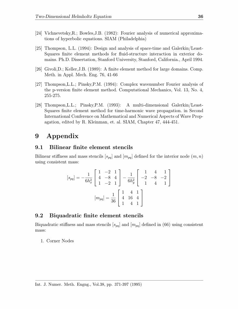
9 Appendix
9.1 Bilinear finite element stencils
Bilinear stiffness and mass stencils [spq] and [mpq] defined for the interior node (m,n)using consistent mass:
[spq] = −1
6h2x
1 −2 14 −8 41 −2 1
− 1
6h2y
1 4 1−2 −8 −21 4 1
[mpq] =1
36
1 4 14 16 41 4 1
9.2 Biquadratic finite element stencils
Biquadratic stiffness and mass stencils [spq] and [mpq] defined in (66) using consistentmass:
1. Corner Nodes
Int. J. Numer. Meth. Engng., Vol.38, pp. 371-397 (1995)
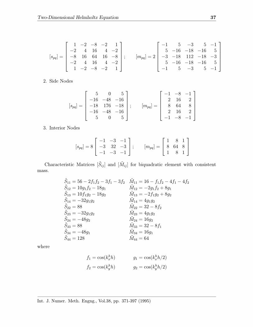
Two-Dimensional Helmholtz Equation 37
[spq] =
1 −2 −8 −2 1−2 4 16 4 −2−8 16 64 16 −8−2 4 16 4 −21 −2 −8 −2 1
; [mpq] = 2
−1 5 −3 5 −15 −16 −18 −16 5−3 −18 112 −18 −35 −16 −18 −16 5−1 5 −3 5 −1
2. Side Nodes
[spq] =
5 0 5−16 −48 −16−18 176 −18−16 −48 −165 0 5
; [mpq] =
−1 −8 −12 16 28 64 82 16 2−1 −8 −1
3. Interior Nodes
[spq] = 8
−1 −3 −1−3 32 −3−1 −3 −1
; [mpq] =
1 8 18 64 81 8 1
Characteristic Matrices [Sij] and [Mij] for biquadratic element with consistentmass.
S11 = 56− 2f1f2 − 3f1 − 3f2 M11 = 16− f1f2 − 4f1 − 4f2S12 = 10g1f2 − 18g1 M12 = −2g1f2 + 8g1S13 = 10f1g2 − 18g2 M13 = −2f1g2 + 8g2S14 = −32g1g2 M14 = 4g1g2S22 = 88 M22 = 32− 8f2S23 = −32g1g2 M23 = 4g1g2S24 = −48g2 M24 = 16g2S33 = 88 M33 = 32− 8f1S34 = −48g1 M34 = 16g1S44 = 128 M44 = 64
where
f1 = cos(khxh) g1 = cos(k
hxh/2)
f2 = cos(khyh) g2 = cos(k
hyh/2)
Int. J. Numer. Meth. Engng., Vol.38, pp. 371-397 (1995)