Knowledge-Based Systems 67 (2014) 49–60

Contents lists available at ScienceDirect

Knowledge-Based Systems

journal homepage: www.elsevier .com/ locate /knosys

A fuzzy logic model for forecasting exchange rates

http://dx.doi.org/10.1016/j.knosys.2014.06.0090950-7051/� 2014 Elsevier B.V. All rights reserved.

⇑ Tel.: +48 583471968.E-mail address: korol.tomasz@gmail.com

Tomasz Korol ⇑Gdansk University of Technology, Faculty of Management and Economics, 80-233 Gdansk, str. Narutowicza 11/12, Poland

a r t i c l e i n f o a b s t r a c t

Article history:Received 1 April 2013Received in revised form 7 May 2014Accepted 9 June 2014Available online 18 June 2014

Keywords:Exchange rateFuzzy logicForecastingFundamental analysisFinancial crisis

This article is devoted to the issue of forecasting exchange rates. The objective of the conducted researchis to develop a predictive model with the use of an innovative methodology – fuzzy logic theory – and toevaluate its effectiveness in times of prosperity (years 2005–2007) and during the financial crisis (years2009–2011).

The model is based on sets of rules written by the author in the form of IF-THEN, where expertknowledge is stored. This model is the result of ten years of the author’s research on this issue.

Empirically, this paper employs three currency pairs as experimental datasets: JPY/USD, GBP/USD andCHF/USD. From the model verification, it is demonstrated that refined processes are effective inimproving the forecasting of exchange rate movements. The author’s created model is characterised byhigh efficiency. These studies are among the world’s first attempts to combine fundamental analysis withfuzzy logic to predict exchange rates.

� 2014 Elsevier B.V. All rights reserved.

1. Introduction

Exchange rates play an important role in international trade,investment determination, risk management in enterprises andthe economic situation of a country by influencing its balance ofpayment. Many countries have implemented a freely floatingexchange rate system that relies upon market mechanisms toadjust the value of their currencies. Currently, interventions of cen-tral banks in a currency market are rare and rarely successful whenattempted. This ineffectiveness implies that market forces influ-ence exchange rates. Exchange rates adjust over time, and a float-ing exchange rate system produces results which, in the long run,reflect the underlying economic fundamentals.

The fluctuation of exchange rates might not be understoodcompletely due to a lack of information about factors affectingthem. Additionally, in the real world, there are times when inputvariables cannot always be determined in the precise sense. There-fore, forecasting exchange rates is often uncertain and vague in anumber of ways. The lack of models capable of providing reliablepredictions of future exchange rates is therefore puzzling. Thispaper takes a novel perspective on the problem and finds an alter-native way of improving the forecasting process by overcoming thedrawbacks contained in statistical models and artificial neural net-works. This paper should offer a good methodology that could beused more easily by investors. In the paper, the author assumes

that there is an effective exchange rate adjustment mechanismoperating in market-based economic systems that employ floatingexchange rates, and Purchasing Power Parity (PPP) and InterestRate Parity (IRP) are part of this mechanism. However, theapproach taken in this paper is different from previously reportedresearch. It brings together two research approaches – the use offuzzy logic (the artificial intelligence method) in combination witha fundamental analysis. Fundamental analysis consists of evaluat-ing the economic and political factors behind currency fluctuationsand involves four theories (they are characterised in detail in Sec-tion 2): Purchasing Power Parity, Interest Rate Parity, the Balanceof Payments Model and the Asset Market Model. The PPP theorystates that exchange rates are determined by the relative pricesof similar sets of goods. The IRP theory states that the fluctuationof one currency against another currency is neutralised by achange in the interest rate differential. While the Balance of Pay-ments Model is mainly focused on stable current account balances,the Asset Market Model is based on financial assets, stating thatexchange rates demonstrate a strong correlation with assetmarkets.

Fuzzy logic provides an appropriate tool for modelling thisimprecise, uncertain and ambiguous phenomenon. Because themovement of exchange rates is affected by many factors (eco-nomic, political, psychological, etc.) that cannot be precisely andunambiguously defined, such an approach greatly enhances thepredictive power of fundamental analysis and makes it an econom-ically useful tool for exchange rate management. The purpose ofthis paper is to improve the forecasting effectiveness of exchange

1 In reality the actual demand and supply of currency depends on several factorssimultaneously. The point of holding all other factors constant is to logically presentthe mechanics how each individual factor influences the exchange rates. Each factorassessed one at a time allows to describe separate influence of each factor onexchange rates. Then, all factors can be tied together to the forecasting model.

50 T. Korol / Knowledge-Based Systems 67 (2014) 49–60

rates with the use of fundamental variables (relative inflation rates,relative interest rates, investments in fixed assets, country ratings,income levels, GDP growth, and trade balance) implemented in thefuzzy logic model.

The paper has the following contribution and innovation to theliterature:

� implementation of fuzzy logic theory into fundamental analysisof the exchange rates,� development of the fuzzy logic models for forecasting the

exchange rates (based on economic factors),� creation of an open application that can be easily updated and

adopted for readers’ needs,� comparative analysis of effectiveness between developed fuzzy

logic models and models of other research approaches (ARCHmodel, GARCH model and artificial neural networks).

Empirically, this paper employs three currency pairs asexperimental datasets. From the model verification, it is shownthat refined processes are effective in improving the forecastingof exchange rate movements.

The paper is organised as follows. Section 2 presents anoverview of the main ways of forecasting exchange rate models.Section 3 recalls the technical background of the fuzzy logic model.Section 4 presents the research assumptions. Section 5 proposesforecasting models for the JPY/USD, GBP/USD and CHF/USD.Section 6 presents the conclusions.

2. Types of forecasting exchange rate models in the literature

The problem of predicting the movement of foreign exchangerates has attracted increasing attention. There are three mainapproaches to forecasting exchange rates in the literature:

(1) The majority of research efforts are devoted to standardmodels, where volatility is a key parameter used withtime-dependent conditional heteroskedasticity. These modelsbelong to the well-known ARCH (autoregressive conditionalheteroskedasticity) and GARCH (generalised autoregressiveconditional heteroskedasticity) approaches initiated by Engle[15] and Bollerslev [4]. The ARCH/GARCH framework has pro-ven to be successful in predicting volatility changes. Thosemodels describe the time evolution of the average size ofsquared errors, that is, the evolution of the magnitude of uncer-tainty Engle et al. [16]. Despite the empirical success of ARCH/GARCH models, there is no real consensus on the economic rea-sons why uncertainty tends to cluster. Therefore, the modelstend to perform better in some periods and worse in other peri-ods. The example of such research is the study conducted byBrandt and Jones [7], which shows that there is substantial pre-dictability in volatility at horizons of up to 1 year, which is incontrast with earlier studies, such as those by West and Cho[46] and Christoffersen and Diebold [13], both of which con-clude that volatility predictability is essentially a short-horizonphenomenon. Additionally, the application of ARCH modelsmay be problematic according to Lamoreux and Lastrapes [28]because ARCH estimates are seriously affected by structuralchanges.(2) Less popular models are those that use a fundamental anal-ysis. These models are based on the information of the supplyand demand and of domestic currency compared with a foreigncurrency. The following factors are the most commonly listedfactors in the literature (for example, [52,31]):(a) Relative inflation rates – changes in relative inflation rates

can affect international trade, which influences the supplyand demand of currencies and therefore affects exchange

rates. A higher inflation rate in country A than in countryB will cause the increase of the import of cheaper productsfrom B to A (ceteris paribus1). This will result in a higherdemand for the currency of country B. At the same time, ahigher relative inflation rate in country A will lead to thereduction of the supply of its currency because the exportof products will decrease in such circumstances. The higherdemand and smaller supply of country A’s currency will leadto the appreciation of country B’s currency. Such findings areconsistent with the conclusions derived from previous stud-ies, for example, those by Parsley and Wei [38] and Qiuet al. [35].

(b) Relative interest rates – changes in relative interest ratesaffect investment in securities, which influences the supplyand demand of currencies. Higher relative interest rates incountry A will lead to a higher supply of currency of countryB in exchange for the currency of country A because invest-ments in securities in country A will be more profitable forinvestors (ceteris paribus). On the other hand, the demandfor currency B should decrease due to less profitable securi-ties. The increase of the supply and the decrease of thedemand of country B’s currency will cause its depreciation.Gruen and Wilkinson [19] find that the real interest rate dif-ferential is qualitatively more important than the balance oftrade in forecasting the exchange rate. Similar conclusionscan be found in recent studies conducted by Chen [10].

(c) Gross domestic product – a country characterised by a highgrowth of GDP should attract foreign investors that willseek to use the opportunities for profit in such an economy.A booming economy in country A would lead to a higherdemand for its currency (ceteris paribus), thereby influenc-ing its appreciation. Karfakis and Phipps [25] and Bergvall[3] report that GDP has a significant influence on exchangerates.

(d) Trade balance – because exports and imports are theelements of GDP, the assumption will be connected to theabove assumption. Increasing the exports of country Ameans that the demand for its currency is increasing, caus-ing its appreciation. Increasing the imports as an opposite toincreasing exports will lead to the depreciation of the cur-rency due to a higher supply of the currency of this country(ceteris paribus). For example, De Gregorio and Wolf [14]demonstrate that an improved balance of trade will leadto an appreciation of the exchange rate.

(e) Income level – higher GDP accompanies high income levels.However, high-income societies tend to increase theirdemand for imported goods. According to this assumption,the growth of the income level in the country will lead tothe depreciation of its currency (ceteris paribus) due tohigher imports. Miyakoshi [34] reveals that the variationin the exchange rate is attributable to the productivity andincome level.

Fundamental analysis has a few drawbacks in forecastingexchange rate movements. Firstly, besides describing the maineconomic variables affecting the supply and demand of thedomestic currency and foreign currencies, there are many otherpsychological and political factors that may lead to speculativetrading. Secondly, different factors can have different impacts onthe exchange rate at different times. There is also empirical

T. Korol / Knowledge-Based Systems 67 (2014) 49–60 51

evidence that presents a low relationship between nominalexchange rate movements and fundamental variables suggestedby the exchange rate determination models (for example,[17,18]). An additional drawback is that in most statisticalmethods, there are some assumptions about the variables used inthe analysis, which cannot be applied to those datasets that donot follow the statistical distributions [12].

(3) The models from the third approach are the least popular in

literature. In recent years, some researchers have implementedartificial intelligence to forecast exchange rates. The most pop-ular artificial intelligence models are artificial neural networks.As a nonparametric and data-driven model, the neural networkmodel imposes few prior assumptions on the underlying pro-cess from which the data are generated [37]. Because of thisproperty, the neural network model is less susceptible to themodel misspecification problem than most parametric statisti-cal models. This does not mean that these models are free fromother defects in forecasting exchange rates. The most commoncomplaint encountered in the literature is the inability to justifythe decision made. Often, the ways in which artificial neuralnetworks make predictions are described as a ‘‘black-box sys-tem’’ [6]. An analysis of the process of assigning individual var-iable weights is complex and difficult to interpret. Neuralnetworks do not provide the course of reasoning leading to acertain assessment, only giving their outcomes without beingable to trace further evidence leading to a final conclusion. Thismakes it difficult to correctly identify the causes of errors gen-erated by an artificial neural network. Another drawback of theuse of artificial neural networks in forecasting exchange rates isan arbitrary method of selecting the network architecture.Although there are general formulas that designate the numberof hidden neurons, the literature postulates the use of an indi-vidual and arbitrary approach for each forecasted phenomenonseparately.

3. Basic concepts of fuzzy logic

Traditional financial models use classical mathematics based onbinary logic. Łukasiewicz [30] named it as the law of bivalence.According to McNeill and Freiberger [33], the law of bivalenceforbids anything other than true and not true responses. In prac-tice, this means that an element (company, phenomenon, etc.)either belongs to a certain set or it does not. There is no third pos-sibility. However, many phenomena in finance are fuzzy, and theyare treated as if they were crisp. Moreover, very often, the inputvariables and data of financial models cannot be determined in aprecise sense. Therefore, fuzzy logic provides an appropriate toolfor modelling imprecise models. The concept of fuzzy logic wasintroduced by Zadeh in 1965. Fuzzy set theory permits the gradualassessment of the membership of elements in relation to a set. Thefuzzy set ‘‘A’’ in a non-empty space X (A # X) can be defined as[49]:

A ¼ fðx;lAðxÞÞjx 2 Xg ð1Þ

where lA: X ? [0,1] is a function of each element of X that deter-mines the extent to which it belongs to set A. This function is calleda membership function of fuzzy set A.

In fuzzy set theory, an element may partially belong to a certainset, and this membership may be expressed by a real number inthe interval [0,1]. Larger values denote higher degrees of set mem-bership. Thus, the membership function lA(x): U) [0,1] is definedas follows [44]:

8x2U lAðxÞ ¼f ðxÞ; x 2 X0; x R X

�ð2Þ

where: lA(x) is a function defining the membership of element x toset A, which is a subset of U; f(x) is a function receiving values fromthe interval [0,1]. The values of this function are called the degreesof membership.

A membership function assigns the degree of membership ofeach element x 2 X to a fuzzy set A, where we can distinguish threesituations:

� lA(x) = 1 means full membership of element x to fuzzy set A,� lA(x) = 0 means that no element x belongs to fuzzy set A,� 0 < lA(x) < 1 means partial membership of an element x to fuzzy

set A.

A fuzzy logic model is constructed by a set of ‘‘IF-THEN’’ rules todescribe the relationship among the input and output variables. Animportant distinguishing feature between fuzzy logic and the tra-ditional expert system is that the rules in fuzzy logic are describedthrough the use of linguistic variables instead of the numericalvariables [51]. Furthermore, in the fuzzy logic model, there is amechanism for describing the degree of membership of an elementto the set and the use of several terms to classify the linguistic vari-ables. For example, a fuzzy logic rule can be stated as follows:

IF the inflation rate is high AND the interest rate is low.THEN the probability of currency depreciation is high.

Where the inflation rate, interest rate and probability of currencydepreciation are linguistic variables, and their terms are high andlow.

With the membership function, all economic phenomena thatcontain a certain part of the lack of precision can be betterdescribed and used in the economic model. For example, thefollowing statements are imprecise:

� The inflation rate is low.� The GDP should increase next year.

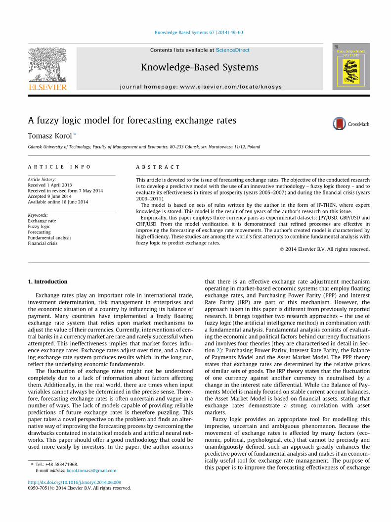
The imprecision of these statements is the inability toaccurately determine the values of all variables occurring in them.When using bivalent logic, an economist is forced to make adecision based on imprecise or fuzzy information, i.e., whetherthe currency will ‘‘appreciate’’ or ‘‘depreciate’’. In the case of theapplication of fuzzy sets, an analyst uses a smooth transitionbetween the total membership [lA(x) = 1] and total non-member-ship [lA(x) = 0] of the analysed phenomenon. The differencebetween classical logic and fuzzy logic in the way of classifyingphenomena is shown in Figs. 1 and 2.

The example of the inflation rate problem in the bivalent model(Fig. 1) can now be represented as a transitional flow from a lowinflation rate to medium inflation rate (Fig. 2). Using fuzzy logic,economists can show how the degree of membership risesbetween 2% and 6%. This way, it eliminates the paradox of thelaw of bivalence with only two possible values ‘‘1 - true’’ or ‘‘0 -false’’ (low or medium inflation rate).

Membership functions can be in any form, arbitrarily deter-mined by the analyst. In the literature, the most common functionstake one of three forms: triangular, trapezoidal or Gaussian.

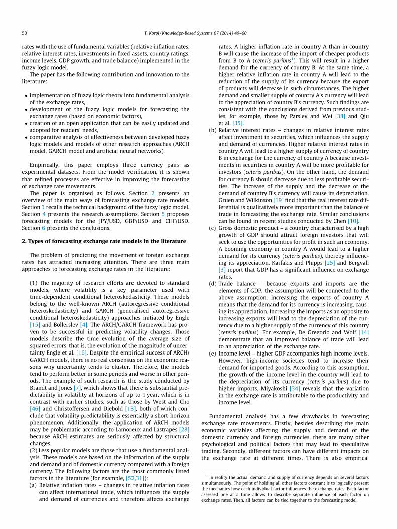
In the case of the trapezoidal membership function (Fig. 3),these functions are defined by four points: a, b, c, and d [44]:

lðxÞ ¼

x�ab�a for a < x < b

1 for b � x � cd�xd�c for c < x < d

0 for x � a or x � d

8>>><>>>:

9>>>=>>>;

ð3Þ

Inflation rate

Degree of membership µ

1

0 5 %

Fig. 1. Classification of the inflation rate using classical logic. Source: Own studybased on Zadeh [50].

8%Interest rates

Degree of membershipμ

04%2% 6%

1

a b c d

Fig. 3. Example of the trapezoidal membership function. Source: Own study basedon Shapiro [41].

a2% Interest rates

Degree of membershipμ

0 8%

1

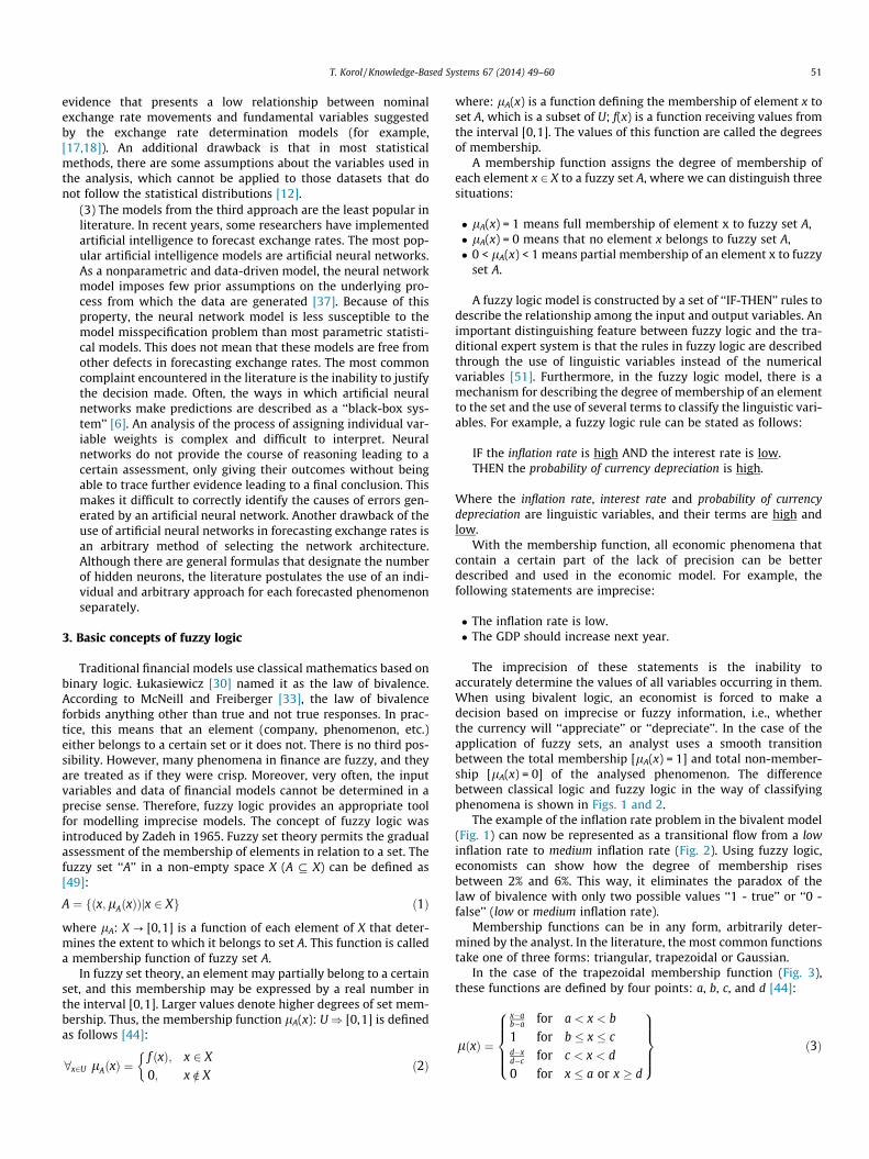
Fig. 4. Example of the Gaussian membership function.

Trade-related factors Investment factors

Investment in fixed assetsTrade balance

52 T. Korol / Knowledge-Based Systems 67 (2014) 49–60

A triangular membership function can be considered as a specialcase of the trapezoidal fuzzy number with b = c.

One-third of the membership function often used is the Gauss-ian curve (Fig. 4). Gaussian functions have the characteristic shapeof a bell with a centre ‘‘a’’ and width ‘‘r’’ dependent parameter:

lðxÞ ¼ e�ðx�aÞ2

r2 ð4Þ

The trapezoidal function can be used to estimate an optimalinterval of the analysed variable (in above example, interest rates).When interest rates are lower than 2%, the situation is classified as‘‘bad’’ (the value is too low). A situation in which the interest ratesreach values greater than 8% is also rated as ‘‘bad’’ (the value is toohigh). Fig. 4 shows an example in which it is assumed that the opti-mum value for the interest rates is at point ‘‘a’’, that is, in the centreof the Gaussian function, values from 2% to 8% belong to varyingdegrees of membership to a set that is ‘‘good’’.

The process to construct a fuzzy logic model generally consistsof three major steps [26]: fuzzification, inference and defuzzifica-tion. Fuzzification arranges numbers by linguistic variables anddefines the types of membership functions for the terms ofvariables. During the second step of constructing the model, theanalyst defines the method of inference. There are two fundamen-tal approaches for the inference procedure: the deductive interpre-tation and the assignment interpretation. The approach that ismost commonly used in practice is the assignment interpretation,and the most common in this category is the Max–Min inference,known as Mandami/Assilian inference, which is based on atriangular minimum norm (TM t-norm; TM(x,y) = min(x,y)) and atriangular maximum conorm (SM t-conorm; SM(x,y) = max(x,y)),that is the dual notion to triangular norm [48,22]. The final stepis representing the defuzzification procedure, which actuallyconverts the fuzzy fact into a fix output value. Three methods ofrealising this procedure are: the MON (mean of maximum), theCOG (centre of gravity) and the COA (centre of area).

Inflation rate

Degree of membership μ

1

0 6% 2 % 3 % 5 %

0.35

0.85

Fig. 2. Classification of the inflation rate using fuzzy logic. Source: Own study basedon Rogers and Labib [40].

The practical applications of fuzzy logic belong more tobusiness administration and engineering than to finance and eco-nomics. Fuzzy logic has recently found extensive applications ina wide variety of industrial systems and consumer products (forexample, [1,47]). Fuzzy logic has also been used in the followingareas of management:

� optimisation of the production processes (for example: [36]),� quality management (for example: [24]),� logistics management (for example: [5]),� inventory management (for example: [11]),

Relative real interest rate

GDP growth

Country rating

Relative inflation rate

Income level

Fig. 5. Out-of-sample economic data.

Table 1Entry variables to the model and their threshold values.

Symbol ofvariable

Description of variable Thresholds for individual membership functions

Description Real value ranges

INT Relative real interest rate:– Between Switzerland and the

USA for forecasting CHF/USD,– Between Japan and the USA

for forecasting JPY/USD,– Between Great Britain and

the USA for forecasting GBP/USD

From �5 percentagepoints (p.p.) to +5 p.p.

Membership functions and its values:– ‘‘Negative’’ – Sigmoidal function: less than 0 p.p. (values less than �4 p.p. belong to the

fuzzy subset ‘‘negative’’ with the degree of membership of 1, values from �4 p.p. to 0p.p. belong to both fuzzy subsets ‘‘negative’’ and ‘‘average’’)

– ‘‘average’’ – Gaussian function: from �4 p.p. to +4 p.p. (values from �4 p.p. to 0 p.p.belong to both fuzzy subsets ‘‘negative’’ and ‘‘average’’; and values from 0 p.p. to +4p.p. belong to fuzzy subsets ‘‘average’’ and ‘‘positive’’)

– ‘‘positive’’ – Sigmoidal function: more than 0 p.p. (values greater than +4 p.p. belong tothe fuzzy subset ‘‘positive’’ with the degree of membership of 1, values from 0 p.p. to +4p.p. belong to both fuzzy subsets ‘‘average’’ and ‘‘positive’’)

GDP Growth rate of GDP:– In Switzerland for forecast-

ing CHF/USD,– In Japan for forecasting JPY/

USD,– In Great Britain for forecast-

ing GBP/USD

From �5% to +5%: Membership functions and its values:– ‘‘Decrease’’ – Sigmoidal function: less than 0% (values less than �2.4% belong to the

fuzzy subset ‘‘decrease’’ with the degree of membership of 1, values from �2.4% to 0%belong to both fuzzy subsets ‘‘decrease’’ and ‘‘steady’’)

– ‘‘Steady’’ – Gaussian function: from �2.4% to +2.4% (values from �2.4% to 0% belong toboth fuzzy subsets ‘‘decrease’’ and ‘‘steady’’; and values from 0% to +2.4% belong to fuzzysubsets ‘‘steady’’ and ‘‘increase’’)

– ‘‘Increase’’ – Sigmoidal function: more than 0% (values greater than +2.4% belong to thefuzzy subset ‘‘increase’’ with the degree of membership of 1, values from 0% to +2.4%belong to both fuzzy subsets ‘‘steady’’ and ‘‘increase’’)

RATING The change of country rating:– Of Switzerland for forecast-

ing CHF/USD,– Of Japan for forecasting JPY/

USD,– Of Great Britain for forecast-

ing GBP/USD

Levels of rating:AAAAA+AAAA�A+AA�BBB+BBBBBB�BB+BBBB�B+BB�

Membership functions and its values:– ‘‘Decrease’’ – Sigmoidal function: less than 0.5 (values less than 0.3 belong to the fuzzy

subset ‘‘decrease’’ with the degree of membership of 1, values from 0.3 to 0.5 belong toboth fuzzy subsets ‘‘decrease’’ and ‘‘steady’’)

– ‘‘Steady’’ – Gaussian function: from 0.3 to 0.7 (values from 0.3 to 0.5 belong to bothfuzzy subsets ‘‘decrease’’ and ‘‘steady’’; and values from 0.5 to 0.7 belong to fuzzy sub-sets ‘‘steady’’ and ‘‘increase’’)

– ‘‘Increase’’ – Sigmoidal function: more than 0.5 (values greater than 0.7 belong to thefuzzy subset ‘‘increase’’ with the degree of membership of 1, values from 0.5 to 0.7belong to both fuzzy subsets ‘‘steady’’ and ‘‘increase’’)

FXAS The dynamics of investments infixed assets:

– In Switzerland for forecast-ing CHF/USD,

– In Japan for forecasting JPY/USD,

– In Great Britain for forecast-ing GBP/USD

From 90% dynamics to120% dynamics

Membership functions and its values:– ‘‘Decrease’’ – Sigmoidal function: less than 105% (values less than 97% belong to the

fuzzy subset ‘‘decrease’’ with the degree of membership of 1, values from 97% to105% belong to both fuzzy subsets ‘‘decrease’’ and ‘‘steady’’)

– ‘‘Steady’’ – Gaussian function: from 97% to 112% (values from 97% to 105% belong toboth fuzzy subsets ‘‘decrease’’ and ‘‘steady’’; and values from 105% to 112% belong tofuzzy subsets ‘‘steady’’ and ‘‘increase’’)

– ‘‘Increase’’ – Sigmoidal function: more than 105% (values greater than 112% belong tothe fuzzy subset ‘‘increase’’ with the degree of membership of 1, values from 105% to112% belong to both fuzzy subsets ‘‘steady’’ and ‘‘increase’’)

INF Relative inflation rate:– Between Switzerland and the

USA for forecasting CHF/USD,– Between Japan and the USA

for forecasting JPY/USD,– Between Great Britain and

the USA for forecasting GBP/USD

From �5 p.p. to +5p.p.

Membership functions and its values:– ‘‘Low’’ –Sigmoidal function: less than 0 p.p. (values less than �2.4 p.p. belong to the

fuzzy subset ‘‘low’’ with the degree of membership of 1, values from �2.4 p.p. to 0p.p. belong to both fuzzy subsets ‘‘low’’ and ‘‘medium’’)

– ‘‘Medium’’ – Gaussian function: from �2.4 p.p. to +2.4 p.p. (values from �2.4 p.p. to 0p.p. belong to both fuzzy subsets ‘‘low’’ and ‘‘medium’’; and values from 0 p.p. to +2.4p.p. belong to fuzzy subsets ‘‘medium’’ and ‘‘high’’)

– ‘‘High’’ – Sigmoidal function: more than 0 p.p. (values greater than +2.4 p.p. belong tothe fuzzy subset ‘‘high’’ with the degree of membership of 1, values from 0 p.p. to+2.4 p.p. belong to both fuzzy subsets ‘‘medium’’ and ‘‘high’’)

TRADE_BAL The growth rate of tradebalance:

– In Switzerland for forecast-ing CHF/USD,

– In Japan for forecasting JPY/USD,

– In Great Britain for forecast-ing GBP/USD

From �10% to +10%: Membership functions and its values:– ‘‘Decrease’’ – Sigmoidal function: less than 0% (values less than �5% belong to the fuzzy

subset ‘‘decrease’’ with the degree of membership of 1, values from �5% to 0% belong toboth fuzzy subsets ‘‘decrease’’ and ‘‘steady’’)

– ‘‘Steady’’ – Gaussian function: from �5% to +5% (values from �5% to 0% belong to bothfuzzy subsets ‘‘decrease’’ and ‘‘steady’’; and values from 0% to +5% belong to fuzzy sub-sets ‘‘steady’’ and ‘‘increase’’)

– ‘‘Increase’’ – Sigmoidal function: more than 0% (values greater than +5% belong to thefuzzy subset ‘‘increase’’ with the degree of membership of 1, values from 0% to +5%belong to both fuzzy subsets ‘‘steady’’ and ‘‘increase’’)

INCOME The growth rate of income level:– In Switzerland for forecast-

ing CHF/USD,– In Japan for forecasting JPY/

USD,

From �5% to +5% Membership functions and its values:– ‘‘Decrease’’ – Sigmoidal function: less than 0% (values less than �2.4% belong to the

fuzzy subset ‘‘decrease’’ with the degree of membership of 1, values from �2.4% to 0%belong to both fuzzy subsets ‘‘decrease’’ and ‘‘steady’’)

(continued on next page)

T. Korol / Knowledge-Based Systems 67 (2014) 49–60 53

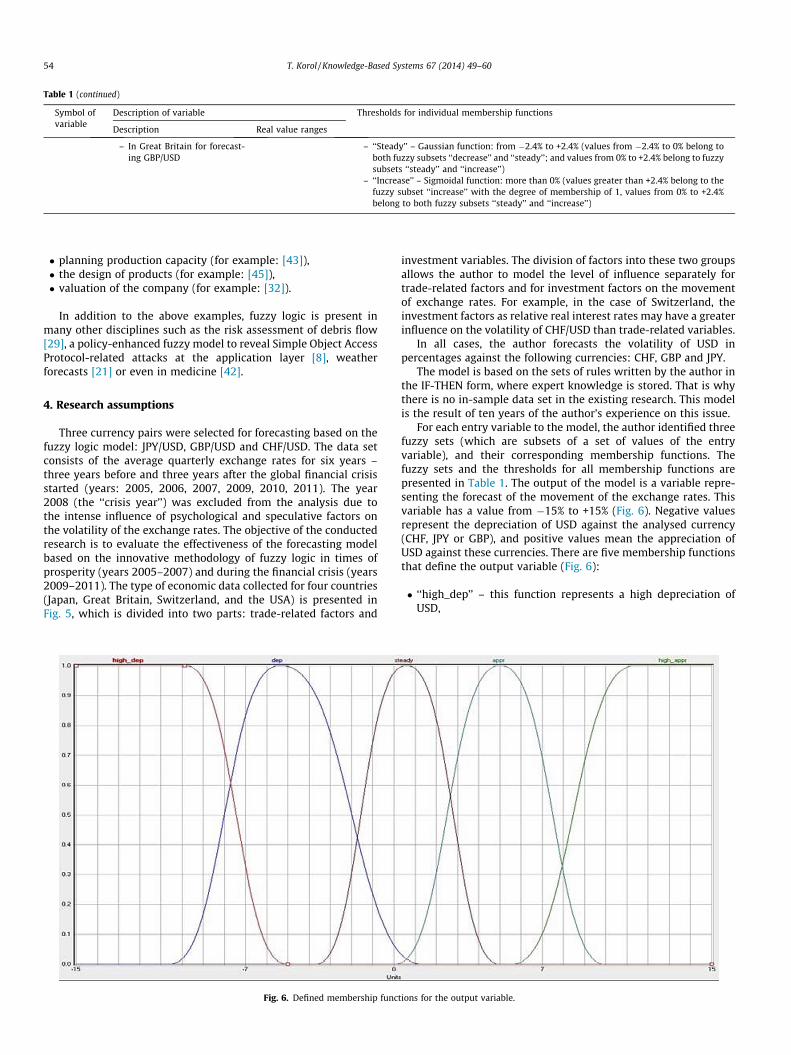
Table 1 (continued)

Symbol ofvariable

Description of variable Thresholds for individual membership functions

Description Real value ranges

– In Great Britain for forecast-ing GBP/USD

– ‘‘Steady’’ – Gaussian function: from �2.4% to +2.4% (values from �2.4% to 0% belong toboth fuzzy subsets ‘‘decrease’’ and ‘‘steady’’; and values from 0% to +2.4% belong to fuzzysubsets ‘‘steady’’ and ‘‘increase’’)

– ‘‘Increase’’ – Sigmoidal function: more than 0% (values greater than +2.4% belong to thefuzzy subset ‘‘increase’’ with the degree of membership of 1, values from 0% to +2.4%belong to both fuzzy subsets ‘‘steady’’ and ‘‘increase’’)

54 T. Korol / Knowledge-Based Systems 67 (2014) 49–60

� planning production capacity (for example: [43]),� the design of products (for example: [45]),� valuation of the company (for example: [32]).

In addition to the above examples, fuzzy logic is present inmany other disciplines such as the risk assessment of debris flow[29], a policy-enhanced fuzzy model to reveal Simple Object AccessProtocol-related attacks at the application layer [8], weatherforecasts [21] or even in medicine [42].

4. Research assumptions

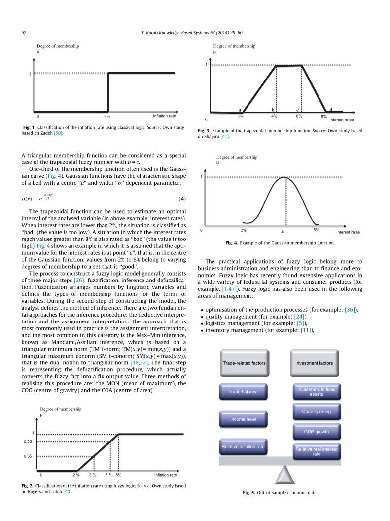
Three currency pairs were selected for forecasting based on thefuzzy logic model: JPY/USD, GBP/USD and CHF/USD. The data setconsists of the average quarterly exchange rates for six years –three years before and three years after the global financial crisisstarted (years: 2005, 2006, 2007, 2009, 2010, 2011). The year2008 (the ‘‘crisis year’’) was excluded from the analysis due tothe intense influence of psychological and speculative factors onthe volatility of the exchange rates. The objective of the conductedresearch is to evaluate the effectiveness of the forecasting modelbased on the innovative methodology of fuzzy logic in times ofprosperity (years 2005–2007) and during the financial crisis (years2009–2011). The type of economic data collected for four countries(Japan, Great Britain, Switzerland, and the USA) is presented inFig. 5, which is divided into two parts: trade-related factors and

Fig. 6. Defined membership func

investment variables. The division of factors into these two groupsallows the author to model the level of influence separately fortrade-related factors and for investment factors on the movementof exchange rates. For example, in the case of Switzerland, theinvestment factors as relative real interest rates may have a greaterinfluence on the volatility of CHF/USD than trade-related variables.

In all cases, the author forecasts the volatility of USD inpercentages against the following currencies: CHF, GBP and JPY.

The model is based on the sets of rules written by the author inthe IF-THEN form, where expert knowledge is stored. That is whythere is no in-sample data set in the existing research. This modelis the result of ten years of the author’s experience on this issue.

For each entry variable to the model, the author identified threefuzzy sets (which are subsets of a set of values of the entryvariable), and their corresponding membership functions. Thefuzzy sets and the thresholds for all membership functions arepresented in Table 1. The output of the model is a variable repre-senting the forecast of the movement of the exchange rates. Thisvariable has a value from �15% to +15% (Fig. 6). Negative valuesrepresent the depreciation of USD against the analysed currency(CHF, JPY or GBP), and positive values mean the appreciation ofUSD against these currencies. There are five membership functionsthat define the output variable (Fig. 6):

� ‘‘high_dep’’ – this function represents a high depreciation ofUSD,

tions for the output variable.

Output Rule block "Output"

Rule Block "Investment"

INT

GDP

RATING

FXAS

Rule Block "Trade"

TRADE_BAL

INCOME

INF

Fig. 7. Diagram of the fuzzy logic model for forecasting exchange rates.

T. Korol / Knowledge-Based Systems 67 (2014) 49–60 55

� ‘‘dep’’ – this function defines an average or low depreciation ofUSD,� ‘‘steady’’ – this function shows the stable situation in the mar-

ket with no significant volatility of USD,

Table 2The set of decision rules of Rule Block ‘‘Investment’’.

Rule Block ‘‘Investment’’

No. IF ‘‘FXAS’’ is: IF ‘‘GDP’’ is: IF ‘‘INT’’ is:

1./2./3. Decrease Decrease Negative4./5. Decrease Decrease Average6. Decrease Decrease Average7./8./9. Decrease Decrease Positive10./11. Decrease Steady Negative12. Decrease Steady Negative13./14./15. Decrease Steady Average16./17. Decrease Steady Positive18. Decrease Steady Positive19./20./21. Decrease Increase Negative22./23. Decrease Increase Average24. Decrease Increase Average25. Decrease Increase Positive26./27. Decrease Increase Positive28./29./30 Steady Decrease Negative31. Steady Decrease Average32./33. Steady Decrease Average34./35./36. Steady Decrease Positive37. Steady Steady Negative38./39 Steady Steady Negative40./41./42. Steady Steady Average43./44. Steady Steady Positive45. Steady Steady Positive46./47./48. Steady Increase Negative49./50. Steady Increase Average51. Steady Increase Average52./53./54. Steady Increase Positive55./56. Increase Decrease Negative57. Increase Decrease Negative58./59./60. Increase Decrease Average61./62. Increase Decrease Positive63. Increase Decrease Positive64./65./66. Increase Steady Negative67./68. Increase Steady Average69. Increase Steady Average70. Increase Steady Positive71./72. Increase Steady Positive73./74./75. Increase Increase Negative76. Increase Increase Average77./78. Increase Increase Average79./80./81. Increase Increase Positive

� ‘‘appr’’ – this function represents an average or low appreciationof USD,� ‘‘high_appr’’ – this function presents the intensive appreciation

of USD.

The author has arbitrarily set fuzzy sets and the shape of mem-bership functions for both entry variables and the output variable.In all cases, Gaussian and Sigmoidal membership functions werechosen. In Table 1, the author specified the type of membershipfunction with its respective range of values for each variable.According to the literature, such functions are the most adequatein representing uncertainty in measurements (for example,[27,20]. Gaussian and Sigmoidal membership functions allowsmooth transition between the full membership [lA(x) = 1] and fullnon-membership [lA(x) = 0] of the analysed variable. Trapezoidalmembership function is good at representing variables that havethe optimal range of values. For example the ratio of current liquid-ity of the enterprise is considered to be optimal in the range [1.2;2.0], the incorrect value belongs to the range (0; 1.2) [ (2.0; 1).When this ratio is less than 1.2, it is considered that the companywill have too low current liquidity; on the other hand, when thisvalue is greater than 2.0 it is said that the company has excessliquidity.

In addition, the most common method for inference waschosen, that is, the Mandami/Assilian inference, and for the

IF ‘‘RATING’’ is: THEN ‘‘INV’’ is:

(1.)Decrease/(2.)Steady/(3.)Increase Increase(4.)Decrease/(5.)Steady IncreaseIncrease Steady(7.)Decrease/(8.)Steady/(9.)Increase Steady(10.)Decrease/(11.)Steady IncreaseIncrease Steady(13.)Decrease/(14.)Steady/(15.)Increase Steady(16.)Decrease/(17.)Steady SteadyIncrease Steady(19.)Decrease/(20.)Steady/(21.)Increase Steady(22.)Decrease/(23.)Steady SteadyIncrease SteadyDecrease Steady(26.)Steady/(27.)Increase Decrease(28.)Decrease/(29.)Steady/(30.)Increase IncreaseDecrease Increase(32.)Steady/(33.)Increase Steady(34.)Decrease/(35.)Steady/(36.)Increase SteadyDecrease Increase(38.)Steady/(39.)Increase Steady(40.)Decrease/(41.)Steady/(42.)Increase Steady(43.)Decrease/(44.)Steady SteadyIncrease Decrease(46.)Decrease/(47.)Steady/(48.)Increase Steady(49.)Decrease/(50.)Steady SteadyIncrease Decrease(52.)Decrease/(53.)Steady/(54.)Increase Decrease(55.)Decrease/(56.)Steady IncreaseIncrease Steady(58.)Decrease/(59.)Steady/(60.)Increase Steady(61.)Decrease/(62.)Steady SteadyIncrease Steady(64.)Decrease/(65.)Steady/(66.)Increase Steady(67.)Decrease/(68.)Steady SteadyIncrease SteadyDecrease Steady(71.)Steady/(72.)Increase Decrease(73.)Decrease/(74.)Steady/(75.)Increase SteadyDecrease Steady(77.)Steady/(78.)Increase Decrease(79.)Decrease/(80.)Steady/(81.)Increase Decrease

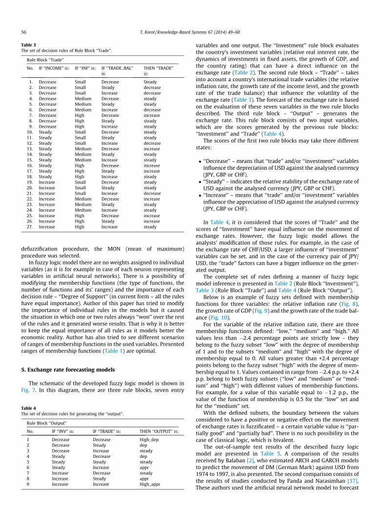
Table 3The set of decision rules of Rule Block ‘‘Trade’’.

Rule Block ‘‘Trade’’

No. IF ‘‘INCOME’’ is: IF ‘‘INF’’ is: IF ‘‘TRADE_BAL’’is:

THEN ‘‘TRADE’’is:

1. Decrease Small Decrease Steady2. Decrease Small Steady decrease3. Decrease Small Increase decrease4. Decrease Medium Decrease steady5. Decrease Medium Steady steady6. Decrease Medium Increase decrease7. Decrease High Decrease increase8. Decrease High Steady steady9. Decrease High Increase steady

10. Steady Small Decrease steady11. Steady Small Steady steady12. Steady Small Increase decrease13. Steady Medium Decrease increase14. Steady Medium Steady steady15. Steady Medium Increase steady16. Steady High Decrease increase17. Steady High Steady increase18. Steady High Increase steady19. Increase Small Decrease steady20. Increase Small Steady steady21. Increase Small Increase decrease22. Increase Medium Decrease increase23. Increase Medium Steady steady24. Increase Medium Increase steady25. Increase High Decrease increase26. Increase High Steady increase27. Increase High Increase steady

56 T. Korol / Knowledge-Based Systems 67 (2014) 49–60

defuzzification procedure, the MON (mean of maximum)procedure was selected.

In fuzzy logic model there are no weights assigned to individualvariables (as it is for example in case of each neuron representingvariables in artificial neural networks). There is a possibility ofmodifying the membership functions (the type of functions, thenumber of functions and its’ ranges) and the importance of eachdecision rule – ‘‘Degree of Support’’ (in current form – all the ruleshave equal importance). Author of this paper has tried to modifythe importance of individual rules in the models but it causedthe situation in which one or two rules always ‘‘won’’ over the restof the rules and it generated worse results. That is why it is betterto keep the equal importance of all rules as it models better theeconomic reality. Author has also tried to see different scenariosof ranges of membership functions in the used variables. Presentedranges of membership functions (Table 1) are optimal.

5. Exchange rate forecasting models

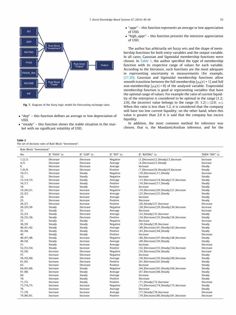
The schematic of the developed fuzzy logic model is shown inFig. 7. In this diagram, there are three rule blocks, seven entry

Table 4The set of decision rules for generating the ‘‘output’’.

Rule Block ‘‘Output’’

No. IF ‘‘INV’’ is: IF ‘‘TRADE’’ is: THEN ‘‘OUTPUT’’ is:

1 Decrease Decrease High_dep2 Decrease Steady dep3 Decrease Increase steady4 Steady Decrease dep5 Steady Steady steady6 Steady Increase appr7 Increase Decrease steady8 Increase Steady appr9 Increase Increase High_appr

variables and one output. The ‘‘Investment’’ rule block evaluatesthe country’s investment variables (relative real interest rate, thedynamics of investments in fixed assets, the growth of GDP, andthe country rating) that can have a direct influence on theexchange rate (Table 2). The second rule block – ‘‘Trade’’ – takesinto account a country’s international trade variables (the relativeinflation rate, the growth rate of the income level, and the growthrate of the trade balance) that influence the volatility of theexchange rate (Table 3). The forecast of the exchange rate is basedon the evaluation of these seven variables in the two rule blocksdescribed. The third rule block – ‘‘Output’’ – generates theexchange rate. This rule block consists of two input variables,which are the scores generated by the previous rule blocks:‘‘Investment’’ and ‘‘Trade’’ (Table 4).

The scores of the first two rule blocks may take three differentstates:

� ‘‘Decrease’’ – means that ‘‘trade’’ and/or ‘‘investment’’ variablesinfluence the depreciation of USD against the analysed currency(JPY, GBP or CHF).� ‘‘Steady’’ – indicates the relative stability of the exchange rate of

USD against the analysed currency (JPY, GBP or CHF).� ‘‘Increase’’ – means that ‘‘trade’’ and/or ‘‘investment’’ variables

influence the appreciation of USD against the analysed currency(JPY, GBP or CHF).

In Table 4, it is considered that the scores of ‘‘Trade’’ and thescores of ‘‘Investment’’ have equal influence on the movement ofexchange rates. However, the fuzzy logic model allows theanalysts’ modification of those rules. For example, in the case ofthe exchange rate of CHF/USD, a larger influence of ‘‘investment’’variables can be set, and in the case of the currency pair of JPY/USD, the ‘‘trade’’ factors can have a bigger influence on the gener-ated output.

The complete set of rules defining a manner of fuzzy logicmodel inference is presented in Table 2 (Rule Block ‘‘Investment’’),Table 3 (Rule Block ‘‘Trade’’) and Table 4 (Rule Block ‘‘Output’’).

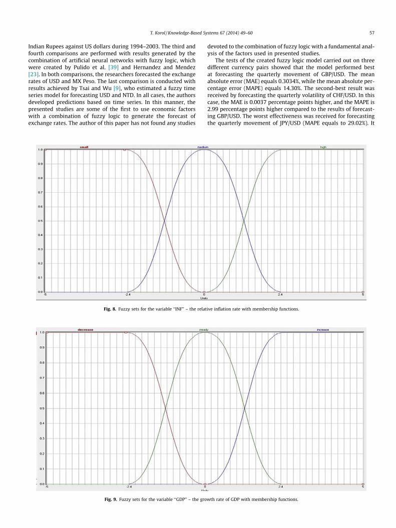
Below is an example of fuzzy sets defined with membershipfunctions for three variables: the relative inflation rate (Fig. 8),the growth rate of GDP (Fig. 9) and the growth rate of the trade bal-ance (Fig. 10).

For the variable of the relative inflation rate, there are threemembership functions defined: ‘‘low,’’ ‘‘medium’’ and ‘‘high.’’ Allvalues less than �2.4 percentage points are strictly low – theybelong to the fuzzy subset ‘‘low’’ with the degree of membershipof 1 and to the subsets ‘‘medium’’ and ‘‘high’’ with the degree ofmembership equal to 0. All values greater than +2.4 percentagepoints belong to the fuzzy subset ‘‘high’’ with the degree of mem-bership equal to 1. Values contained in range from �2.4 p.p. to +2.4p.p. belong to both fuzzy subsets (‘‘low’’ and ‘‘medium’’ or ‘‘med-ium’’ and ‘‘high’’) with different values of membership functions.For example, for a value of this variable equal to �1.2 p.p., thevalue of the function of membership is 0.5 for the ‘‘low’’ set andfor the ‘‘medium’’ set.

With the defined subsets, the boundary between the valuesconsidered to have a positive or negative effect on the movementof exchange rates is fuzzificated – a certain variable value is ‘‘par-tially good’’ and ‘‘partially bad’’. There is no such possibility in thecase of classical logic, which is bivalent.

The out-of-sample test results of the described fuzzy logicmodel are presented in Table 5. A comparison of the resultsreceived by Balaban [2], who estimated ARCH and GARCH modelsto predict the movement of DM (German Mark) against USD from1974 to 1997, is also presented. The second comparison consists ofthe results of studies conducted by Panda and Narasimhan [37].These authors used the artificial neural network model to forecast

T. Korol / Knowledge-Based Systems 67 (2014) 49–60 57

Indian Rupees against US dollars during 1994–2003. The third andfourth comparisons are performed with results generated by thecombination of artificial neural networks with fuzzy logic, whichwere created by Pulido et al. [39] and Hernandez and Mendez[23]. In both comparisons, the researchers forecasted the exchangerates of USD and MX Peso. The last comparison is conducted withresults achieved by Tsai and Wu [9], who estimated a fuzzy timeseries model for forecasting USD and NTD. In all cases, the authorsdeveloped predictions based on time series. In this manner, thepresented studies are some of the first to use economic factorswith a combination of fuzzy logic to generate the forecast ofexchange rates. The author of this paper has not found any studies

Fig. 8. Fuzzy sets for the variable ‘‘INF’’ – the relat

Fig. 9. Fuzzy sets for the variable ‘‘GDP’’ – the gro

devoted to the combination of fuzzy logic with a fundamental anal-ysis of the factors used in presented studies.

The tests of the created fuzzy logic model carried out on threedifferent currency pairs showed that the model performed bestat forecasting the quarterly movement of GBP/USD. The meanabsolute error (MAE) equals 0.3034%, while the mean absolute per-centage error (MAPE) equals 14.30%. The second-best result wasreceived by forecasting the quarterly volatility of CHF/USD. In thiscase, the MAE is 0.0037 percentage points higher, and the MAPE is2.99 percentage points higher compared to the results of forecast-ing GBP/USD. The worst effectiveness was received for forecastingthe quarterly movement of JPY/USD (MAPE equals to 29.02%). It

ive inflation rate with membership functions.

wth rate of GDP with membership functions.

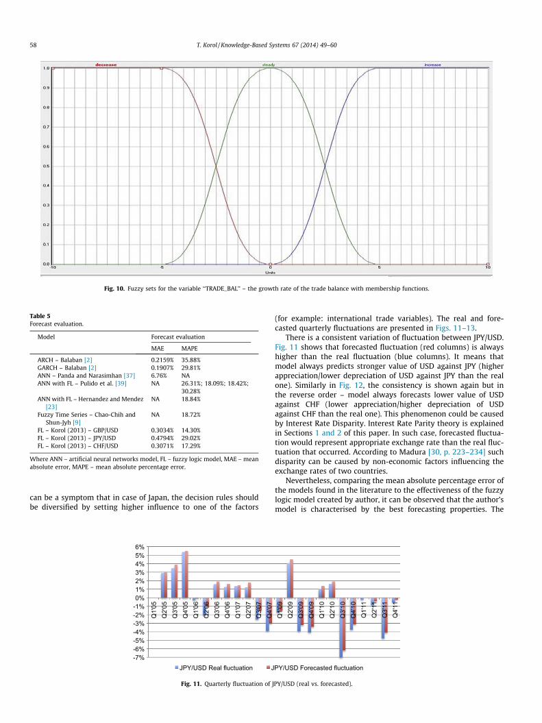
Fig. 10. Fuzzy sets for the variable ‘‘TRADE_BAL’’ – the growth rate of the trade balance with membership functions.

Table 5Forecast evaluation.

Model Forecast evaluation

MAE MAPE

ARCH – Balaban [2] 0.2159% 35.88%GARCH – Balaban [2] 0.1907% 29.81%ANN – Panda and Narasimhan [37] 6.76% NAANN with FL – Pulido et al. [39] NA 26.31%; 18.09%; 18.42%;

30.28%ANN with FL – Hernandez and Mendez

[23]NA 18.84%

Fuzzy Time Series – Chao-Chih andShun-Jyh [9]

NA 18.72%

FL – Korol (2013) – GBP/USD 0.3034% 14.30%FL – Korol (2013) – JPY/USD 0.4794% 29.02%FL – Korol (2013) – CHF/USD 0.3071% 17.29%

Where ANN – artificial neural networks model, FL – fuzzy logic model, MAE – meanabsolute error, MAPE – mean absolute percentage error.

58 T. Korol / Knowledge-Based Systems 67 (2014) 49–60

can be a symptom that in case of Japan, the decision rules shouldbe diversified by setting higher influence to one of the factors

-7% -6% -5% -4% -3% -2% -1% 0% 1% 2% 3% 4% 5% 6%

Q1'

05

Q2'

05

Q3'

05

Q4'

05

Q1'

06

Q2'

06

Q3'

06

Q4'

06

Q1'

07

Q2'

07

Q3'

07

Q4'

07

JPY/USD Real fluctuation J

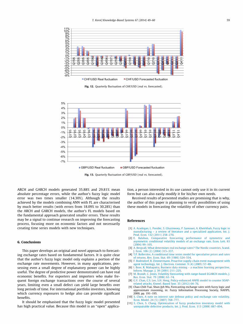
Fig. 11. Quarterly fluctuation of J

(for example: international trade variables). The real and fore-casted quarterly fluctuations are presented in Figs. 11–13.

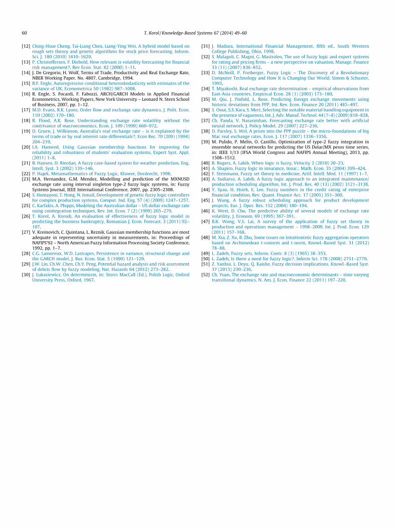
There is a consistent variation of fluctuation between JPY/USD.Fig. 11 shows that forecasted fluctuation (red columns) is alwayshigher than the real fluctuation (blue columns). It means thatmodel always predicts stronger value of USD against JPY (higherappreciation/lower depreciation of USD against JPY than the realone). Similarly in Fig. 12, the consistency is shown again but inthe reverse order – model always forecasts lower value of USDagainst CHF (lower appreciation/higher depreciation of USDagainst CHF than the real one). This phenomenon could be causedby Interest Rate Disparity. Interest Rate Parity theory is explainedin Sections 1 and 2 of this paper. In such case, forecasted fluctua-tion would represent appropriate exchange rate than the real fluc-tuation that occurred. According to Madura [30, p. 223–234] suchdisparity can be caused by non-economic factors influencing theexchange rates of two countries.

Nevertheless, comparing the mean absolute percentage error ofthe models found in the literature to the effectiveness of the fuzzylogic model created by author, it can be observed that the author’smodel is characterised by the best forecasting properties. The

Q1'

09

Q2'

09

Q3'

09

Q4'

09

Q1'

10

Q2'

10

Q3'

10

Q4'

10

Q1'

11

Q2'

11

Q3'

11

Q4'

11

PY/USD Forecasted fluctuation

PY/USD (real vs. forecasted).

-8% -7% -6% -5% -4% -3% -2% -1% 0% 1% 2% 3% 4% 5% 6% 7% 8% 9%

10% 11%

Q1'

05

Q2'

05

Q3'

05

Q4'

05

Q1'

06

Q2'

06

Q3'

06

Q4'

06

Q1'

07

Q2'

07

Q3'

07

Q4'

07

Q1'

09

Q2'

09

Q3'

09

Q4'

09

Q1'

10

Q2'

10

Q3'

10

Q4'

10

Q1'

11

Q2'

11

Q3'

11

Q4'

11

CHF/USD Real fluctuation CHF/USD Forecasted fluctuation

Fig. 12. Quarterly fluctuation of CHF/USD (real vs. forecasted).

-7% -6% -5% -4% -3% -2% -1% 0% 1% 2% 3% 4% 5%

Q1

'05

Q2

'05

Q3

'05

Q4

'05

Q1

'06

Q2

'06

Q3

'06

Q4

'06

Q1

'07

Q2

'07

Q3

'07

Q4

'07

Q1

'09

Q2

'09

Q3

'09

Q4

'09

Q1

'10

Q2

'10

Q3

'10

Q4

'10

Q1

'11

Q2

'11

Q3

'11

Q4

'11

GBP/USD Real fluctuation GBP/USD Forecasted fluctuation

Fig. 13. Quarterly fluctuation of GBP/USD (real vs. forecasted).

T. Korol / Knowledge-Based Systems 67 (2014) 49–60 59

ARCH and GARCH models generated 35.88% and 29.81% meanabsolute percentage errors, while the author’s fuzzy logic modelerror was two times smaller (14.30%). Although the resultsachieved by the models combining ANN with FL are characterisedby much better results (with errors from 18.09% to 30.28%) thanthe ARCH and GARCH models, the author’s FL models based onthe fundamental approach generated smaller errors. These resultsmay be a signal to continue research on improving the forecastingprocess, focusing more on economic factors and not necessarilycreating time series models with new techniques.

6. Conclusions

This paper develops an original and novel approach to forecast-ing exchange rates based on fundamental factors. It is quite clearthat the author’s fuzzy logic model only explains a portion of theexchange rate movements. However, in many applications, pos-sessing even a small degree of explanatory power can be highlyuseful. The degree of predictive power demonstrated can have realeconomic benefits. For exporters and importers who make fre-quent foreign exchange transactions over the course of severalyears, limiting even a small defect can yield large benefits overlong periods of time. For international portfolio investors, knowingwhich currency exposures to hedge also can provide significantbenefits.

It should be emphasised that the fuzzy logic model presentedhas high practical value. Because this model is an ‘‘open’’ applica-

tion, a person interested in its use cannot only use it in its currentform but can also easily modify it for his/her own needs.

Received results of presented studies are promising that is why,the author of this paper is planning to verify possibilities of usingthese models in forecasting the volatility of other currency pairs.

References

[1] A. Azadegan, L. Porobic, S. Ghazinoory, P. Samouei, A. Kheirkhah, Fuzzy logic inmanufacturing – a review of literature and a specialized application, Int. J.Prod. Econ. 132 (2011) 258–270.

[2] E. Balaban, Comparative forecasting performance of symmetric andasymmetric conditional volatility models of an exchange rate, Econ. Lett. 83(2004) 99–105.

[3] A. Bergvall, What determines real exchange rates? The Nordic countries, Scand.J. Econ. 106 (2) (2004) 315–337.

[4] T.P. Bollerslev, A conditional time series model for speculative prices and ratesof returns, Rev. Econ. Stat. 69 (1986) 524–554.

[5] F. Bodendorf, R. Zimmermann, Proactive supply-chain event management withagent technology, Int. J. Electron. Commer. 9 (4) (2005) 57–89.

[6] I. Bose, R. Mahapatra, Business data mining – a machine learning perspective,Inform. Manage. J. 39 (2001) 211–225.

[7] M. Brandt, C. Jones, Volatility forecasting with range-based EGARCH models, J.Bus. Econ. Stat. 79 (2006) 61–74.

[8] G.Y. Chan, C.S. Lee, S.H. Heng, Policy-enhanced ANFIS model to counter SOAP-related attacks, Knowl.-Based Syst. 35 (2012) 64–76.

[9] Chao-Chih Tsai, Shun-Jyh Wu, Forecasting exchange rates with fuzzy logic andapproximate reasoning, in: Fuzzy Information Processing Society, NAFIPS,2000, pp. 191–195.

[10] S. Chen, A note on interest rate defense policy and exchange rate volatility,Econ. Model. 24 (5) (2007) 768–777.

[11] S. Chen, S. Chang, Optimization of fuzzy production inventory model withunrepairable defective products, Int. J. Prod. Econ. 113 (2008) 887–894.

60 T. Korol / Knowledge-Based Systems 67 (2014) 49–60

[12] Ching-Hsue Cheng, Tai-Liang Chen, Liang-Ying Wei, A hybrid model based onrough sets theory and genetic algorithms for stock price forecasting, Inform.Sci. J. 180 (2010) 1610–1629.

[13] P. Christoffersen, F. Diebold, How relevant is volatility forecasting for financialrisk management?, Rev Econ. Stat. 82 (2000) 1–11.

[14] J. De Gregorio, H. Wolf, Terms of Trade, Productivity and Real Exchange Rate,NBER Working Paper. No. 4807, Cambridge, 1994.

[15] R.F. Engle, Autoregressive conditional heteroskedasticity with estimates of thevariance of UK, Econometrica 50 (1982) 987–1008.

[16] R. Engle, S. Focardi, F. Fabozzi, ARCH/GARCH Models in Applied FinancialEconometrics, Working Papers, New York University – Leonard N. Stern Schoolof Business, 2007, pp. 1–12.

[17] M.D. Evans, R.K. Lyons, Order flow and exchange rate dynamics, J. Polit. Econ.110 (2002) 170–180.

[18] R. Flood, A.K. Rose, Understanding exchange rate volatility without thecontrivance of macroeconomics, Econ. J. 109 (1999) 660–972.

[19] D. Gruen, J. Wilkinson, Australia’s real exchange rate – is it explained by theterms of trade or by real interest rate differentials?, Econ Rec. 70 (209) (1994)204–219.

[20] I.A. Hameed, Using Gaussian membership functions for improving thereliability and robustness of students’ evaluation systems, Expert Syst. Appl.(2011) 1–8.

[21] B. Hansen, D. Riordan, A fuzzy case-based system for weather prediction, Eng.Intell. Syst. 3 (2002) 139–146.

[22] P. Hajek, Metamathematics of Fuzzy Logic, Kluwer, Dordrecht, 1998.[23] M.A. Hernandez, G.M. Mendez, Modelling and prediction of the MXNUSD

exchange rate using interval singleton type-2 fuzzy logic systems, in: FuzzySystems Journal, IEEE International Conference, 2007, pp. 2305–2308.

[24] S. Homayoni, T. Hong, N. Ismail, Development of genetic fuzzy logic controllersfor complex production systems, Comput. Ind. Eng. 57 (4) (2009) 1247–1257.

[25] C. Karfakis, A. Phipps, Modeling the Australian dollar – US dollar exchange rateusing cointegration techniques, Rev. Int. Econ. 7 (2) (1999) 265–279.

[26] T. Korol, A. Korodi, An evaluation of effectiveness of fuzzy logic model inpredicting the business bankruptcy, Romanian J. Econ. Forecast. 3 (2011) 92–107.

[27] V. Kreinovich, C. Quintana, L. Reznik, Gaussian membership functions are mostadequate in representing uncertainty in measurements, in: Proceedings ofNAFIPS’92 – North American Fuzzy Information Processing Society Conference,1992, pp. 1–7.

[28] C.G. Lamoreux, W.D. Lastrapes, Persistence in variance, structural change andthe GARCH model, J. Bus. Econ. Stat. 5 (1990) 121–129.

[29] J.W. Lin, Ch.W. Chen, Ch.Y. Peng, Potential hazard analysis and risk assessmentof debris flow by fuzzy modeling, Nat. Hazards 64 (2012) 273–282.

[30] J. Łukasiewicz, On determinism, in: Storrs MacCall (Ed.), Polish Logic, OxfordUniversity Press, Oxford, 1967.

[31] J. Madura, International Financial Management, fifth ed., South WesternCollege Publishing, Ohio, 1998.

[32] S. Malagoli, C. Magni, G. Mastroleo, The use of fuzzy logic and expert systemsfor rating and pricing firms – a new perspective on valuation, Manage. Finance33 (11) (2007) 836–852.

[33] D. McNeill, P. Freiberger, Fuzzy Logic – The Discovery of a RevolutionaryComputer Technology and How It is Changing Our World, Simon & Schuster,1993.

[34] T. Miyakoshi, Real exchange rate determination – empirical observations fromEast-Asia countries, Empirical Econ. 28 (1) (2003) 173–180.

[35] M. Qiu, J. Pinfold, L. Rose, Predicting foreign exchange movements usinghistoric deviations from PPP, Int. Rev. Econ. Finance 20 (2011) 485–497.

[36] S. Onut, S.S. Kara, S. Mert, Selecting the suitable material handling equipment inthe presence of vagueness, Int. J. Adv. Manuf. Technol. 44 (7–8) (2009) 818–828.

[37] Ch. Panda, V. Narasimhan, Forecasting exchange rate better with artificialneural network, J. Policy Model. 29 (2007) 227–236.

[38] D. Parsley, S. Wei, A prism into the PPP puzzle – the micro-foundations of bigMac real exchange rates, Econ. J. 117 (2007) 1336–1356.

[39] M. Pulido, P. Melin, O. Castillo, Optimization of type-2 fuzzy integration inensemble neural networks for predicting the US Dolar/MX pesos time series,in: IEEE 1/13 (IFSA World Congress and NAFIPS Annual Meeting), 2013, pp.1508–1512.

[40] B. Rogers, A. Labib, When logic is fuzzy, Velocity 2 (2010) 20–23.[41] A. Shapiro, Fuzzy logic in insurance, Insur.: Math. Econ. 35 (2004) 399–424.[42] F. Steinmann, Fuzzy set theory in medicine, Artif. Intell. Med. 11 (1997) 1–7.[43] A. Sudiarso, A. Labib, A fuzzy logic approach to an integrated maintenance/

production scheduling algorithm, Int. J. Prod. Res. 40 (13) (2002) 3121–3138.[44] Y. Syau, H. Hsieh, E. Lee, Fuzzy numbers in the credit rating of enterprise

financial condition, Rev. Quant. Finance Acc. 17 (2001) 351–360.[45] J. Wang, A fuzzy robust scheduling approach for product development

projects, Eur. J. Oper. Res. 152 (2004) 180–194.[46] K. West, D. Cho, The predictive ability of several models of exchange rate

volatility, J. Econom. 69 (1995) 367–391.[47] B.K. Wong, V.S. Lai, A survey of the application of fuzzy set theory in

production and operations management – 1998–2009, Int. J. Prod. Econ. 129(2011) 157–168.

[48] M. Xia, Z. Xu, B. Zhu, Some issues on intuitionistic fuzzy aggregation operatorsbased on Archimedean t-conorm and t-norm, Knowl.-Based Syst. 31 (2012)78–88.

[49] L. Zadeh, Fuzzy sets, Inform. Contr. 8 (3) (1965) 38–353.[50] L. Zadeh, Is there a need for fuzzy logic?, Inform Sci. 178 (2008) 2751–2779.[51] Z. Yanhui, L. Deyu, Q. Kaishe, Fuzzy decision implications, Knowl.-Based Syst.

37 (2013) 230–236.[52] Ch. Yuan, The exchange rate and macroeconomic determinants – time varying

transitional dynamics, N. Am. J. Econ. Finance 22 (2011) 197–220.