A Foundation Model for Marxian Breakdown Theories Basedon a New Falling Rate of Profit Mechanism (Long Version)

By Howard Petith*

July 2002

Address: Departament d’Economia i d’Història Econòmica, Edifici B, UniversitatAutònoma de Barcelona, 08193 Bellaterra (Barcelona) Spain. Howard.Petith@uab.es

Abstract: The paper presents a foundation model for Marxian theories of thebreakdown of capitalism based on a new falling rate of profit mechanism. All of thesetheories are based on one or more of “the historical tendencies”: a rising capital-wagebill ratio, a rising capitalist share and a falling rate of profit. The model is a foundationin the sense that it generates these tendencies in the context of a model with a constantsubsistence wage. The newly discovered generating mechanism is based on neo-classical reasoning for a model with land. It is non-Ricardian in that land augmentingtechnical progress can be unboundedly rapid. Finally, since the model has no steadystate, it is necessary to use a new technique, Chaplygin’s method, to prove the result.

JEL Classification: B24,E11,O41

I. Introduction.

1. The Point of the Paper.

The point of the paper is to supply a foundation model for Marxian theories of the

breakdown of capitalism. All of these breakdown theories are based on one or more of

what Dumenil and Levy (2000) have dubbed the historical tendencies, that is a rising

ratio of capital to the wage bill, a rising share of capital1 and a falling rate of profit. The

model is a foundation in the sense that it generates each of these tendencies. Of course

the model would have to be added to in different ways in order to supply the analytic

counterpart of each of the theories.

2. The Model.

* This paper first appeared as a working paper of the UAB in 1992 and has accumulated numerous debtsin its development. Thanks go to Hamid Azari, Jordi Brandts, Roberto Burguet, Ramon Caminal, GerardDuménil, Simon Emsley, Ducan Foley, Alan Freeman, John Hamilton, and Carmen Matutes. Thanks fortheir comments go also to the participants of the following meetings where it was presented: TheBellaterra Seminar, the Macro Workshop at the UAB, The Atlantic International Economic Conference,El Simposio de Análisis Económico, the IWGVT Conference, Nuevas Direcciones en el PensamientoEconómico and the conference on New and Old Growth Theories. The paper has also greatly benefitedfrom numerous anonymous criticisms for which the author is grateful. Finally thanks go to DeirdreHerrick for her considerable help. Financial support from Dirección General de Investigación project #SEC2000-0684 is acknowledged

1 The Marxian terms are the composition of capital and the rate of exploitation respectively.

2

The model has one sector with a CES production function in land and a capital-

labour aggregate, each of which experiences factor augmenting technical progress at a

different rate. The labour supply is infinitely elastic at a subsistence wage. Capitalists

own the land as well as capital which accumulates because of capitalist savings. The

result is that, if the elasticity of substitution between land and the capital-labour

aggregate is less than one, then the model generates the historical tendencies.

The model has no steady state and the result refers to the general characteristics of

non-steady state behaviour. Because of the absence of a steady state it is necessary to

use a new technique, Chaplygin’s method, in the proof.

3. The Mechanism.

The basic contribution of the paper is the discovery of a new mechanism which

generates a falling rate of profit. There are two mechanisms which have been said to

cause a falling rate of profit in models of this type: The Marxian explanation which

involves a growing capital-wage bill ratio in the context of a model with no land2 and a

Ricardian explanation which is based on growing land scarcity and the existence of a

class of landlords.3

The mechanism set out here is different from both of these. It is different from the

Marxian one since it involves land in a crucial way. It is also different from the

Ricardian one since it does not depend on technical progress in land being slower than

that in the capital-labour aggregate, nor on the existence of a landlord class which soaks

up profits via rents.

Roughly the mechanism works as follows. Suppose, for example, that the rate of

technical progress in land is greater than that in the capital-labour aggregate. If only

technical progress were taken into account, in efficiency units, land would grow faster

than capital. But the more rapid growth of land causes income, savings and thus capital

to grow more rapidly. The sum of these two sources, technical progress and saving, is

sufficient, under the stated condition, to ensure that capital grows faster than land. This

in turn causes the rate of profit to fall.

4. Breakdown Theories.4

2 This explanation is now generally acknowledged to be incorrect. See Howard and King (1992 chap. 7)for a description of the voluminos literature. Marx also propounded a secondary Ricardian-likeexplanation. See Petith (2001b).3 Ricardo (1963, Chaps II and VI). Blaug (1988, Chap. 4) gives a summary.4 The information in this section is taken from Part III of Petith (2001a) which describes the historicaldevelopment of these theories. Part III in turn is taken from Clarke (1994) for Marx, and Howard andKing (1989,1992) for Marxist writers.

3

The theories can be divided into those that have capitalism ending as a result of an

evermore violent series of business cycles (called crises) and those that have it ending

because of trends. In the business cycle group the first theory argues that the rise in the

capital-wage bill ratio will cause a continual shift of demand from consumption to

investment goods, that supply will not adequately react and that the resulting over

supply of consumption goods will lead to increasingly violent business cycles. An

additional part of this theory is that the falling rate of profit will cause increasingly risky

investment ventures to be chosen which will add to the amplitude of the cycles. The

second theory works through the rising capital share. Since capitalists are thought to

invest rather than consume this continually increases the proportion of aggregate

demand that is devoted to investment. Since investment demand is more volatile, this

increases the instability of the economy and leads to more violent fluctuations.

In the trend group the first is that capitalists will put pressure on workers as they try

to avoid the fall of their rate of profit and that this will increase social conflict. The

second is that the rise in the capital-wage bill ratio will somehow make large holdings

of capital more efficient and thus centralise ownership. This, combined with the rising

share of capital, will cause an increasingly unequal distribution of income with ever

fewer increasingly wealthy capitalists on the one hand and growing mass of

impoverished workers on the other. The third is that the composition of capital will rise

in a way to ensure that there is a sufficiently large number of unemployed workers,

called the reserve army, to keep the wages from rising about subsistence level. The last

is that the rate of profit will fall to such an extent that capitalism itself will not be viable.

These descriptions show that all of the breakdown theories depend on one or more of

the historical tendencies.

5. The Model as a Foundation.

Since the model is meant to serve as a foundation, it is important that the model does

not contradict the general idea of each of the theories and that it allows the important

aspects of the theories to be set out analytically. In this, as will be seen, the model is

only partially successful.

First, consider the subsistence wage assumption. Marx was ambivalent about

whether the real wage would rise or not, and sections of his writings can be cited to

support either position. A number of writers have reproduced some or all of the

4

historical tendencies in models with rising wages.5 But when one is constructing a

background for breakdown theories, I think that a subsistence wage is a far better

assumption for two reasons: First, the basic Marxian notion that capitalism will

breakdown because of class antagonism is much less convincing in the context of rising

wages; and second, three out of four of the tendency theories actually postulate

impoverishment of the working class.

Second, consider the assumption that capitalists own the land. Marx’s writing contain

large sections which describe the actions of landlords and there can be no doubt that he

viewed the economy as divided into three classes as did Ricardo.6 But since none of the

breakdown theories involves landlords, the assumption seems harmless.

Third, consider the theories one by one. Clearly the model is unsuitable for the third

trend group theory: One can not have a reserve army when the infinitely elastic supply

of labour implies there will be no unemployment. A different approach is needed. The

two business cycle theories need a two sector model, but it would seem that the falling

rate of profit mechanism would work in this case so that only a modification would be

needed. Finally the remaining three trend theories would seem to fit into the unmodified

model.

Thus, while it is not perfect, the model seems well suited to its task.

6. The Importance of the Model.

At first glance, it would seem idle to construct breakdown models when capitalism is

in obvious good health, but a deeper look shows that this is not the case. First, the

models would be directly relevant for third world capitalist countries where the

instability and conflictive class relations that these theories describe reflect the actual

conditions. Second, the models could serve as an analytic framework for the

descriptions of actual revolution s have followed from Skocpol’s seminal work (1979).7

And finally, with respect to current first world capitalism, models of contingent

breakdown could be constructed8 which would explore the fragility of its current

success.9

5 See Laibman (1977, 1997), Duménil and Lévy (1993,1995,2000), Skott (1992), Michl (1994, 1999) andSkillman (1997).6 See Marx (1954 Parts V and VI).7 Skocpol developed an analytic methodology and used it to analyse the French, Russian and Chineserevolutions. This line has been developed further by Popkin (1988) for Vietnam, by Wickham-Crowley(1992) for Latin America and Renner (1997) for southern Mexico and Zaire among others.8 Petith (2000) and Foley (2000) are examples: In the first case, a fall in the rate of technical progress andin the second, a failure of account for environmental externalities switch the paths of the models from a

5

7. The Relation to the Literature.

The model of this paper together with those of Petith (2000) and Foley (2000) are the

only ones to have generated the historical tendencies in the context of a non-rising

wage. The 1970’s and early 1980’s saw the construction of a number of formal Marxian

models, but the absence of land and the infinitely elastic supply of labour robbed them

of any dynamics.10 In the 1990’s a number of Marxist writers developed models of the

falling rate of profit but always in the context of a rising wage. 11 Petith (2000) has a

constant capital share and a profit rate that falls only on the approach to steady state.

Foley (2000) has a simulation model which appears to exhibit the historical tendencies

together with a falling wage, but this aspect is not emphasised. Thus the present model

appears to be somewhat of a break-though.

The rest of the paper is organised as follows: Section II sets out the model and a

statement of the result, Section III gives a heuristic explanation of the mechanism and

Section IV provides the proof.

II. The Model and the Result.

The specific production function that produces output Y is CES in a Cobb-Douglas

capital/labour aggregate and land, where K, L, and M are capital, labour and land.

(1) Y=[α(KβL1-βeγt)-ρ+(1-α)(Meδt)-ρ]-1/ρ

The aggregate experiences factor augmenting technical progress at rate γ > 0 while landexperiences it at rate δ ≥ 0. The elasticity of substitution between the aggregate and land

is σ = 1

1 + ρ , -1 ≤ ρ ≤ ∞ , where α, βε [0, 1] are parameters and t is time. The constant

real wage w and the rental on capital are equal to their respective marginal products,(2) w = ∂Y/∂L

(3) r = ∂Y/∂K.

The rate of return on investment in land, which is its marginal product plus the capital

gain P•

divided by the price, is equal to the return on capital,12

neo-classical to a Marxian mode. Galor and Moave (2000) are a reverse example: They have capitalistself interested provision of education saving capitalism from the Marxist scenario.9 Another important aspect of the model which falls outside the thrust of the paper is that it provides anexplanation for an important empirical regularity. The full result states that the rate of profit will rise orfall as the elasticity of substitution is greater or less that one. All models that I know of have the rate ofprofit converging to a steady state value. But the empirical reality is that, at least for the United States, therate of profit has experienced large long term fluctuations. See Dumenil, Glick and Rangel (1987).10 See Morishima (1973), Steadman (1977), Roemer (1981) and Marglin(1984).11 See footnote 5 for references.

12 x•

is the derivative of x with respect to time.

6

(4) r =∂Y

∂M+ P

•

/ P ,

where P is the price of land in terms of the good. Capitalists are assumed to own the

land as well as capital. Their rate of profit R is defined as

(5) R =Y + P

•M − wL

K + PM .

It is easily shown that r = R and from this point on r will be called the rate of profit.

Savings are provided only by capitalists who save all their income13. Their savings are

equal to the accumulation of wealth,

(6) P•

M + K•

= Y + P•

M − wL .

The assumption that all profits are saved removes P•

M from the accumulation equation

and immensely simplifies the model. Finally the definitions of the capital-wage bill ratio

k and a measure of the capitalist share (or rate of exploitation) e are given by14

k =K

wL, e =

Y

wL−1.

This concludes the presentation of the model.

The model yields a single differential equation in K in the following manner. (2)

determines L as a function of K and t, L(K,t). Thus output also depends on these two

variables, Y(K,L,t) = Y(K,L(K,t),t). Substituting these into (6) gives the non-autonomous

differential equation

(7) K•

= f(K,t) K(t0) = K0 > 0

where K0, the initial capital stock, is assumed to be positive. The initial-value problem

(7) has a solution K(t). Taking account of the dependence of L on K and t, this solution

implies the time paths of the key variables, k(t), r(t) and e(t) as well as the extensive

ones Y, K and L.

The characteristics of these time paths are given by the following theorem.

13 This assumption is discussed in the following section.14 e without an exponent is the measure of the capitalist share. e with an exponent is the ordinarymathematical symbol.

7

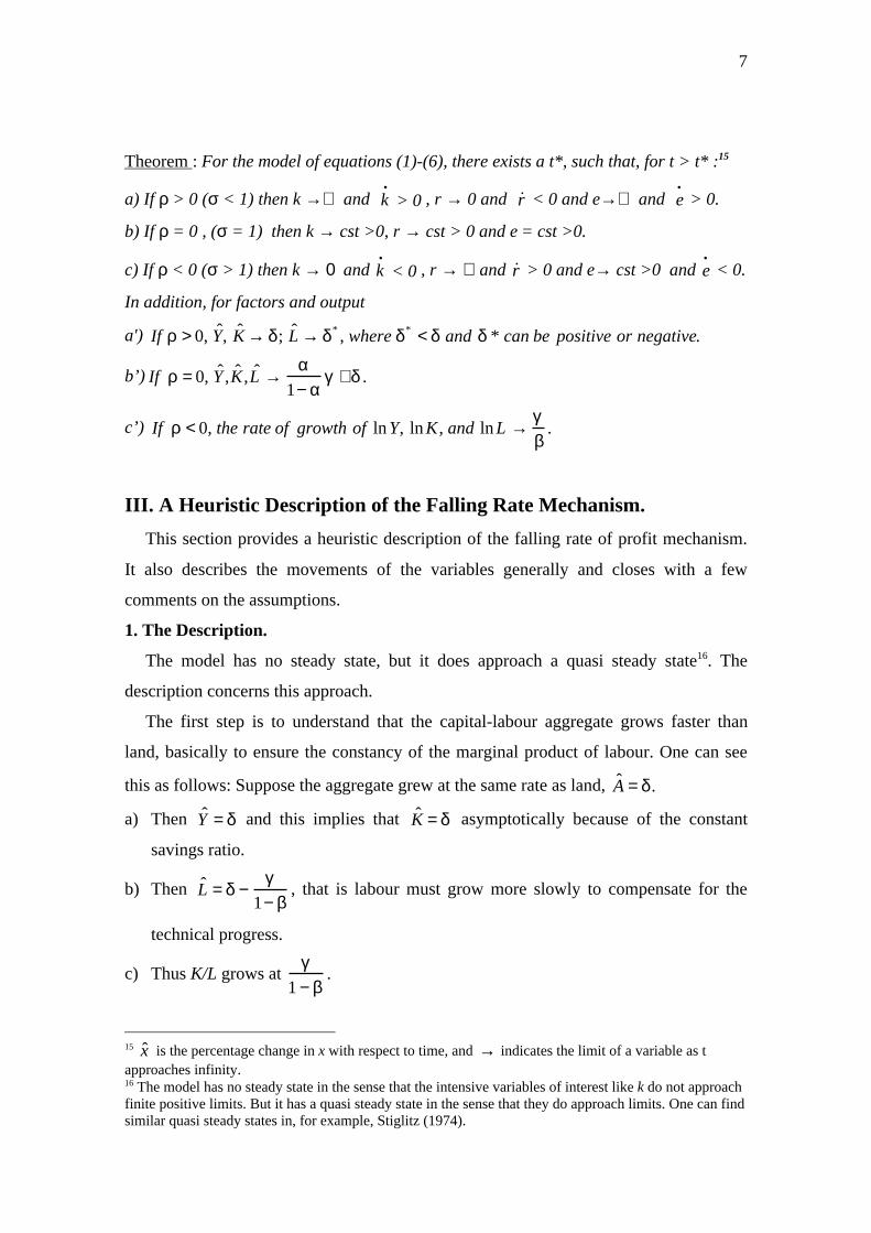
Theorem : For the model of equations (1)-(6), there exists a t*, such that, for t > t* :15

a) If ρ > 0 (σ < 1) then k →∝ and k• > 0 , r → 0 and ˙ r < 0 and e→∝ and e

• > 0.

b) If ρ = 0 , (σ = 1) then k → cst >0, r → cst > 0 and e = cst >0.

c) If ρ < 0 (σ > 1) then k → 0 and k• < 0 , r → ∝ and ˙ r > 0 and e→ cst >0 and e

• < 0.

In addition, for factors and output

a') If ρ > 0, ˆ Y , ˆ K → δ ; ˆ L → δ * , where δ * < δ and δ * can be positive or negative.

b’) If ρ = 0, ˆ Y , ˆ K , ˆ L →α

1− αγ +δ .

c’) If ρ < 0, the rate of growth of ln Y, ln K , and ln L →γβ

.

III. A Heuristic Description of the Falling Rate Mechanism.

This section provides a heuristic description of the falling rate of profit mechanism.

It also describes the movements of the variables generally and closes with a few

comments on the assumptions.

1. The Description.

The model has no steady state, but it does approach a quasi steady state16. The

description concerns this approach.

The first step is to understand that the capital-labour aggregate grows faster than

land, basically to ensure the constancy of the marginal product of labour. One can see

this as follows: Suppose the aggregate grew at the same rate as land, ˆ A = δ .

a) Then ˆ Y = δ and this implies that ˆ K = δ asymptotically because of the constant

savings ratio.

b) Then ˆ L = δ −γ

1− β, that is labour must grow more slowly to compensate for the

technical progress.

c) Thus K/L grows at γ

1 − β.

15 ˆ x is the percentage change in x with respect to time, and → indicates the limit of a variable as tapproaches infinity.16 The model has no steady state in the sense that the intensive variables of interest like k do not approachfinite positive limits. But it has a quasi steady state in the sense that they do approach limits. One can findsimilar quasi steady states in, for example, Stiglitz (1974).

8

d) Thus the marginal product of labour, which is proportional to K

L

β

eγt , grows at

β1 − β

γ + γ =γ

1− β > 0, which is impossible.

e) Thus labour must grow faster than the expression given in b) and the aggregate

grows faster than land, ˆ A > δ

Note that the rate of profit only depends on K/L . This because the ratio of the

marginal products depends only on K/L and the wage is fixed. Thus a rise in K/L implies

that the rate of profit falls.

Consider what happens when σ<1. In this case the slowest growing factor dominates

so that ˆ Y = ˆ K = δ . Suppose that K/L is constant, then ˆ A = δ + γ .Then the ratio of the

aggregate to land rises at γ. Because σ<1, the marginal product of labour falls at more

that γ but only rises at γ. Thus the marginal product of labour falls which is impossible.

Labour must grow more slowly, K/L rises and the rate of profit falls. To complete this

case note that the capitalist share approaches 1 because the share of land approaches 1

and the capitalists own it. Finally note that this is an exogenous growth model in the

sense that output grows at δ , a rate determined by the exogenous technical progress.

Now consider what happens when σ>1. In this case the fastest growing factor

dominates and the aggregate essentially detaches itself from land:

w =K

L

β

1 − β( )eγt .

K/L has to fall to keep the wage constant, the rate of profit rises and the share of capital

falls to that given by the Cobb-Douglas. Finally, because of the infinitely elastic labour

supply, production is linear in capital alone so that the model is, asymptotically, one of

endogenous growth.17 However, because there is also exogenous technical progress, it is

the rate of growth of output that grows at a constant rate.

2. Comments.

The basic characteristic of the mechanism is the rapid growth of the aggregate. This,

in turn, depends on the assumptions of the infinitely elastic supply of labour and the

17 For example, if all capital gains were saved but only a proportion of profits, then the rate of growthwould depend on that proportion.

9

constant saving proportion.18 It would be good to know if the result would survive the

weakening of these assumptions.

With respect to the second, a natural weakening would be the introduction of utility

maximisation. If an overlapping generations framework was adopted, it seems likely

that the result could be preserved. On the other hand, if an infinite horizon framework

was used,19 the outcome would be more problematic. It is unlikely that a general result

would come out of a more complicated model so simulation would have to be resorted

to20. In this case the present paper can be thought of as the first prong of a two pronged

attack: a general result for a simple model plus the investigation of more general models

in terms of specific examples.

IV. The Proof (Referee A).21

1. The Differential Equation.

It seems impossible to write the differential equation (7) without side conditions. But

this can be done for the variable x.

(8) x = KβL1− βeγ −δ( )t .

The differential equation is then

(9) ˙ x = eϕ tF x( ) + G x( ) with initial condition x t0( ) = x0 > 0

where F x( ) =aµx xρ + βc2( )

c2 + x ρ( )µ / ρc2 + µxρ( )

, G x( ) = ϕ − δ( )x c2 + xρ( )c2 + µxρ , µ =

1+ ρ − βρβ

and a, c1 and c2 are positive constants. The variables of interest depend on x as

follows:

(10) Y = eδ t f x( )

(11) L =1 − β

weδ t xf ' x( )

18 As noted in the previous footnote, the savings proportion out of profits need not be 1 so that capitalistsmay eat. It is the constancy that is important.19 It might seem that the perfect foresight that is usually assumed is a bad assumption for a model of theend of capitalism. But if this impedes the functioning of the mechanism, then capitalism will not end andthe assumption will be justified.20 Foley (2000) is an example of this approach.21 This proof, somewhat modified, is the one worked out by referee A of JEBO for the paper Petith(2001a). The referee’s exact proof is set out in that paper. The proofs are different here because, at thetime, no one realised that the theorem was true without a restriction on the rate of technical progress inland. I saw this while studying the referee’s proof.

10

(12) K =w

1− β

1−ββ

eδ −ϕ( ) t x

f ' x( )( ) 1− β( ) / β

(13) r = β1 − β

w

1−β( ) / β

eϕ t f ' x( )( )1/ β

(14) k =β

1 - β1

r

(15) e =1

1 − βc2 + xρ

c2

−1

where f x( ) =c1x

c2 + xρ( )1/ ρ and ϕ =γβ

.22 Once the asymptotic behaviour of x is

found, the theorem follows from equations (10)-(15).

First, Lemma 1 gives some general characteristics of the solution to (9). Then the

proof of the theorem is given only for the case where ρ>1 and φ-δ<0. (The proofs for

the other cases are given in Petith (2002).) This is the most important case since it

shows that the historical tendencies emerge in spite of rapid technical progress in

agriculture. It is also the more difficult case.

2. Lemma 1.

When ϕ-δ<0 the characteristics and even the existence of a solution to (9) are

problematic. Let x(t) be this solution. In this case it may be that ˙ x t( )<0 so that x(t)<0 is

a possibility. This, in turn, would lead to three difficulties: First, x(t)<0 has no

economic meaning. To see the remaining difficulties which are technical, let ρ=a/b ,

where a and b are real numbers. If a is odd and b is even then x t( )ρ is imaginary and

F(x) is complex. If both a and b are odd then xr<0, F(x) → - ∞ as x→ −c2

1

ρ and the

existence of a solution on [t0, ∞) is doubtful. Lemma 1 shows that x(t)>0, that x(t) is

defined on [t0, ∞) and, in addition, demonstrates a few other useful characteristics of the

solution.

It uses the following results from Grimshaw (1990).

Lemma (page 8). If g(x,t) is a continuous function of x and t in the product domain for

which xε D and tε I and the partial derivative ∂g /∂x exists and is bounded for all x in

the convex domain D and all t ε I, then g satisfies a Lipschitz condition with the

Lipshitz constant

22 These calculations are set out in Appendix I.

11

L = maxD,I

∂g

∂x.

Here and below I is an open interval and D is an open connected set.

Theorem 1.4 (Picard iteration). Let g(x,t) be continuous for

t − t0 ≤ α, x − x0 ≤ β

and satisfy a Lipschitz condition with constant L in this region. Let g x,t( ) ≤ M there

and let δ = min [α, β/Μ]. Then the initial value problem

˙ x = g x,t( ), x t0( ) = x0

has a unique solution for t − t0 ≤ δ .

Theorem 1.7. Let g(x,t) be continuous for x in the domain D and t in the open interval I,

and satisfy a Lipschitz condition there. Then, for any point xo in D and t0 in I, the initial

value problem

˙ x = g x,t( ), x t0( ) = x0

has a unique solution x(t) which is defined for t0 ≤ t < T (T ≤∞) and is such that, if T<∞,

then either x t( ) → ∞ as t →T or (x(t),t) approaches the boundry of the product domain

(D,I) as t → T .

These results are now used to prove Lemma 1.

Lemma 1. The solution to (9) exists and is unique on [t0, ∞). Let x(t) be the solution,

then x(t)>0, t ≥t0 and x(t) is unbounded above.

Proof: Modify (9) in two steps. The first step is to write (9) as

(9’) ˙ x = eϕ tF x( ) + G x( ) x t0( ) = x0 .

Note that this is different from (9), but only when x<0. The second step is to change the

variable to y = xe−ϕt . Then we have

(9’’) ˙ y = g y,t( ) y t0( ) = y0

where g y,t( ) = F yeϕt( ) + e−ϕtG yeϕt( ) − ϕ ye−ϕt and y0 = x0e−ϕ t . g(y, t) is continuous on

(-∞, ∞)x(0,∞) and ∂g /∂y exists and is bounded on this domain. It follows from the

lemma (page 8) that g(y, t) satisfies a Lipshitz condition on this domain. Thus it follows

from Theorem 1.7 that (9’’) has a unique solution y(t) for t0≤t<T.

Suppose that y(t) = 0 for some values of t. Then, since y(t) is continuous and y(t0)>0,

there exists a t such that y( t )=0 and y(t)>0 for t0≤t< t . Note that y(t) is also a solution

to the initial value problem

(16) ˙ y = g y,t( ), y t ( ) = 0 .

12

Now choose α and β so that the conditions t − t ≤ α, y − 0 ≤ β imply that (y,

t)εDxI. Then the conditions of theorem 1.4 are satisfied on this region and y(t),

t − t ≤ δ is the unique solution to (16). But by observation, y t( ), y t ( ) = 0, t − t ≤ δ is

also a solution to (16). Since y (t)≠ y(t), this contradicts the uniqueness. Thus y(t)=0 for

no value of t and by continuity y(t)>0 for t0≤t<T.

It follows that (9’) has a unique solution x(t)=y(t)eϕ t defined on t0≤t<T and that

x(t)>0. Since (9’) is identical to (9) for x>0 , it follows that (9) has the same solution as

(9’) on the same domain of t.

Next to show that x(t) is defined on [t0, ∞), write g(.) as

(17) g x,t( ) =a

xµ xeϕt ˜ F x( ) +ϕ − δ

µx ˜ G x( )

where ˜ F x( ) =µx µ xρ + βc2( )

c2 + x ρ( )µρ c2 + µxρ( )

and ˜ G x( ) =µ c2 + x ρ( )c2 + µxρ . Note that

(18) limx →∞

˜ F x( ) = limx → ∞

˜ G x( ) = 1.

Suppose that T<∞, then by theorem 1.7, x(t)→∞ as t →T, since it is impossible that

(x, t) approaches the boundary of the product domain. Choose ˜ t such that x(t)>1 for

t≥ ˜ t . Then one can find A such that

A >a

xµ eϕt ˜ F x( ) +ϕ −δ

µ˜ G x( ) t ≤ T

so that ˙ x = g x,t( ) < Ax. Integrating gives ln x T( ) < A T − ˜ t ( ) + ln x ˜ t ( ) which contradicts

the approach of x to infinity. Thus x(t) is defined on [t0, ∞).

Finally suppose that x(t) is bounded above, x(t)<x*. First suppose that ϕ−δ<0.

Clearly there is a G such that G > ˜ G (x(t), t) for all t. Furthermore x does not approach

0 as t→∞ since, if it did, limt →∞

˙ x ≤ 0; but in this case, i.e. when x→0, limt →∞

g x t( ),t( ) > 0 .

Thus, since x(t) is continuous and x(t)>0, it is possible to find x>0 such that x(t)>x,

t0≤t<∞. Thus one can find F< ˜ F (x(t), t), to≤t<∞. The existence of F , G and x* allows

one to write

g x t( ),t( ) >a

x *( )µ eϕt F +ϕ − δ

µG

x t( ) .

Let t* such that the expression in the square brackets for this value of t, A, is positive.

Thus g(x(t),t)>Ax(t), t≥t*. Integration from t to t* gives lnx( t )>lnx(t*)+A( t -t*),

x( t )→∞ as t →∞ which contradicts the assumption that x(t) was bounded above.

13

Second let ϕ−δ>0 . Then a similar argument can be constructed by finding G such that

G(x(t), t)>G for t*≤t<∞.

3. The Proofs of the Theorem for the Three Cases.

a. ρ>0 and ϕ-δ<0.

The structure of the argument can be read from figure 1. Lemma 2 uses Chaplygin’s

theorem to establish that x eventually lies between two bounding functions, xMT and xmT.

tTTT

x

x

X

MT

mT

x

x----

x

1 2

ε

ε

Figure 1. The illustration of lemmas 2 and 3.

14

Lemma 3 then shows that the bounding functions eventually enter the ε tube

surrounding a known path x . Thus x is asymptotically equivalent to x .

Theorem (Chaplygin)23 For an equation of the form ˙ x =g(x,t), x(T)=X, if the

differential inequalities

˙ x mT(t)-g(xmT(t),t)<0

˙ x MT(t)-g(xMT(t),t)>0

hold with t>T and xmt(T)=xMT(T)=X, then

xmT(t)<x(t)<xMT(t)

holds for all t>T.

A few preliminaries are necessary. It is clear that

(19) ˜ G (x)/ ˜ F (x) >1,

(20) there exists x such that ˜ F ’(x)<0, ˜ G ’(x)<0, ( ˜ G (x)/ ˜ F (x))’<0 for x> x .

Next consider the equation that is the limit of (9) as x→∞. Using (17) and (18), this is

(21) ˙ x =a

xµ −1 eϕt +ϕ − δ

µx, x T( ) = X .

This has the solution24

(22) x (t;a,δ,T,X)=aµδ

eϕ t 1− eδtC a,δ , X,T( )[ ]

1

µ

whereC .( ) = eδT 1 −δXµ

aµeϕT

.

(21) also has an asymptotic solution:

(23) x t( ) =aµδ

eϕt

1

µ.

Differentiating (22) gives

(24) ˙ x t( ) =1

µx

1

µ−1 aµ

δeϕt ϕ + δ − ϕ( )C .( )e−δt[ ].

It is possible to modify equation (21) in two ways:

(25)

˙ x =a

xµ −1eϕt + m

ϕ − δµ

x , x t( ) = X

= a

xµ −1eϕt + ϕ −δm

µx

23 See Mikhlin and Smolitskiy (1967) pp.9-12 or Zwillinger (1989) pp. 388-91.24 Set out in Appendix II.

15

where δm=δ m+(1-m)ϕ; and

(26)

˙ x = Ma

x µ −1eϕ t +

ϕ −δµ

x

, x T( ) = X

= aM

xµ −1eϕt + ϕ −δ M

µx

where aM=Ma and δM=δM+(1-M)ϕ. Equations (25) and (26) have the solution given by

(22) with a and δ modified appropriately.

Lemma 2. Let x(t) be the solution to (9) and let ρ>0 and ϕ-δ<0. For any ˜ x there exists a

T such that x(T)> ˜ x and

x mT(t)<x(t)< x MT(t), t>T

where x mT(t)= x (t;a,δm,x(T),T), m= ˜ G (x(T))/ ˜ F (x(T))

x MT(t)= x (t;aM,δM,x(T),T), M= ˜ G (T).

Proof: For the given ˜ x choose T so that x(T)> ˜ x , so that x(T)> x of (20), and so that

˙ x (T)>0. This is possible since, by lemma 1, x(t) is unbounded above. Since ˙ x (T)>0 ,

looking at (17),

(27)a

xµ −1 eϕt ˜ F x( ) +ϕ − δ

µx ˜ G x( ) > 0, x = x T( ),

by (20)

˙ x mT T( ) =a

xµ −1 eϕT +ϕ − δ

µx

˜ G x( )˜ F x( ) > 0, x = xmT T( )

and from (24)

(28) ˙ x mT t( ) > 0, t ≥ T.

Also from (27)

˙ x MT T( ) = ˜ G x( ) a

x µ −1 eϕ t +ϕ −δ

µx

>

˜ G x( )˜ F x( )˜ G x( )

a

xµ −1 eϕt +ϕ − δ

µx

> 0 for x = xMT T( )

by (19), and from (24)

(29) ˙ x MT t( ) > 0, t ≥ T.

Now it is shown that the conditions of Chaplygin’s theorem are satisfied:

x mT(T)=x(T)= x MT(T)

by construction.

(30) x mT(t)> x mT(T), x MT(t)> x MT(T) for t>T

by (28) and (29).

16

˙ x mT t( ) =a

xµ −1eϕt + m

ϕ −δµ

x <a

xµ −1eϕt +

˜ G x( )˜ F x( )

ϕ −δµ

x

˜ F x( )

= a

xµ −1eϕt ˜ F x( ) + ϕ −δ

µx ˜ G x( ) for x = xmT t( ), t > T

by (18), (20), (28) and (30).

˙ x MT t( ) = Ma

xµ −1eϕt +

ϕ −δµ

x

>˜ F x( )˜ G x( )

a

xµ −1eϕt +

ϕ −δµ

x

˜ G x( )

= axµ −1

eϕt ˜ F x( ) + ϕ −δµ

x ˜ G x( ), for x = xMT t( ), t > T

by (19), (20), (29) and (30). This completes the proof.

Lemma 3. Let x(t) be the solution to (9) and let ρ>0 and ϕ-δ<0. Then

limt →∞

x t( )x t( ) =1.

Proof: Choose ε >0 arbitrary but with ε <1, ε < 4/δϕ

−1

. It must be shown that there

is a Tε such that

1 − ε( )x t( ) < x t( ) < 1 + ε( )x t( ), t > Tε .

Choose ˜ x large enough so that for the T given by lemma 2

(31)˜ G x( )˜ F x( ) < 1+

ε / 2

1 −ϕ / δ, ˜ G x( ) < 1+

1ϕδ

1 + ε / 4

ε / 4−1

for x > x T( ).

Now apply lemma 2. The proof is completed by showing that there exists a Tε such that

1 − ε( )x t( ) < xmT t( ), xMT t( ) < 1 + ε( )x t( ), t > Tε .

Choose T1 >T so that

1 − ε / 2( ) <1 − eδm tC a,δm , x T( ),T( ), t > T1 .

(31) implies

1

1 + ε / 2<

1

m + 1− m( )ϕ /δ.

1 − ε( )µ < 1 −ε( ) < 1

1+ ε / 21− ε / 2( ) < 1

δm / δ1 − ε / 2( )

1 − ε( )µ aµδ

eϕt <aµδm

eϕt 1− eδmtC a,δm ,x T( ),T( )[ ]1 − ε( )x t( ) < xmT t( ) for t > T1.

Choose T2 >T such that

1 − eδ M tC aM ,δM , x T( ),T( ) < 1+ ε / 4.

17

(31) implies

M

M + 1 − M( )ϕ / δ<1 + ε / 4 .

aM

δM

<a

δ1 + ε / 4( )

aMµδM

eϕ t 1− eδM tC aM ,δM , x T( ),T( )[ ] <aµδ

eϕt 1+ ε / 4( )2

<aµδ

eϕt 1+ ε( ) <aµδ

eϕt 1 + ε( )µ , t > T2 .

xMT t( ) < 1 + ε( )x t,( ) t > T2 .

The proof is completed by taking Tε=max(T1, T2).

Proof of the theorem for the case ρ>0, ϕ-δ<0: From lemma 3

x t( ) =aµδ

1

µe

ϕµ

t

asymptotically. The proof is completed by substituting this into equations (10)-(15).

b. ρ>0 and ϕ-δ>0.

The proof follows the lines of the previous case but is more simple. Again it is

possible to modify equation (21) as

(32) ˙ x = λaeϕ t

x µ −1 +ϕ −δ

µx

with the initial condition x T( ) = X.

=aλeϕ t

x µ −1 +ϕ −δλ

µx

with aλ = λa and δλ = λδ + 1 -λ( )ϕ which has the solution given by (22) with a and δ

modified appropriately.

Next one has the equivalent of Lemma 2.

Lemma 2’. Let ρ>0 and ϕ−δ>0. If x(t) is the solution of equation (9), if T > t0 , and if m

and M satisfy:

(33) m < ˜ F x( ) < M and m < ˜ G x( ) < M if x > x T( )then

(34) x m ,T t( ) < x t( ) < x M,T t( ) if t > T

with x m ,T t( ) = x t;am ,δm ,T ,x T( )( ) and x M ,T t( ) = x t; aM ,δM ,T, x T( )( ).Proof:

18

Since x(t) satisfies equation (9) with x(t0)=x0 > 0 and ϕ-δ>0 , ˙ x t( ) is always positive

and x(t) is increasing and positive. The same is true of x m ,T and x M ,T which satisfy

equation (32) with the initial condition x m ,T T( ) = x M ,T T( ) = x T( ) > 0, which are also

increasing functions. It follows that x m ,T t( ) and x M ,T t( ) are strictly larger than x(T) for

t > T. Consequently, using equations (32), (33) and (17), one has

˙ x m ,T = maeϕ t

x m ,T( )µ −1 +ϕ −δ

µx m, T

<

aeϕ t

x m ,T( )µ −1˜ F x m, T( ) +

ϕ −δµ

x m, T˜ G x m,T( )=eϕ t F x m,T( ) + G x m ,T( )

as well as:

˙ x M,T > eϕ tF x M,T( ) + G x M, T( ). Chaplygins’s conditions are satisfied, and this brings the proof of equation (34) to

completion.

Finally one has the equivalent of Lemma 3.

Lemma 3’. Let ρ>0 and ϕ-δ>0, if x(t) is the solution of (16), then:

limx →∞

x t( )x t( ) = 1.

Proof:

We want to prove that, for any ε (which can be assumed to be smaller than 1), one can

find Tε such that

1 − ε( )x t( ) < x t( ) < 1 + ε( )x t( ) ∀t > Tε .

We define:

(35) ν = 3 + 4ϕ −δ

δ.

Since ˜ F x( ) and ˜ G x( ) tend to 1 when x tends to infinity, Xε exists such that:

1 −εν

< ˜ F x( ) < 1+εν

and 1 −εν

< ˜ G x( ) <1 +εν

∀x > Xε .

We define Tε1 by x Tε

1( ) = Xε , and apply the lemma for T = Tε1 and for :

(36) m = 1−εν

and M = 1 +εν

.

We must now prove that a value of Tε can be determined such that:

(37) 1 − ε( )x t( ) < x m ,T t( ) and x M, T t( ) < 1 + ε( )x t( ) ∀t > Tε .

1. With ν defined by equation (35), ϕ−δ larger than 0, m and M defined by equation

(36) and ε smaller than 1, one can prove that:

19

1−ε3

a

δ<

am

δm

and aM

δM

< 1 +ε3

a

δ.

2. If Cm,T and CM,T are the two constants in the expressions of x m ,T t( ) and x M ,T t( ) :

Cm,T =C(am ,δm T, x(T)) and CM,T =C(aM ,δM T, x(T))

and defining Tε2 and Tε

3 by:

Cm ,Tε

1 e−δ mTε2

=ε3

and CM ,Tε

1 e− δM Tε3

,

then one has:

1 −ε3

<1 − Cm ,Tε

1e−δ mt and 1− C

M ,Tε1e

−δ M t <1 +ε3

∀t > max Tε2,Tε

3( ).

3. Since µ is larger than 1, or 1/µ smaller than 1, and still assuming that ε is smaller

than 1, one has:

1 − ε < 1 − ε( )1/ µ < 1−ε3

2

1/ µ

and 1+ε3

2

1/ µ

< 1 + ε( )1/ µ < 1+ ε .

Choosing Tε = max Tε1,Tε

2 ,Tε3( ), the inequalities (37) are satisfied, and this brings the

proof of Lemma 3’ to completion.

Proof of the theorem for the case ρ>0, ϕ-δ>0: From lemma 3’

x t( ) =aµδ

1

µe

ϕµ

t

asymptotically. The proof is completed by substituting this into equations (10)-(15).

c. ρ<0.

This case differs from the preceding two in that it is the rate of growth of the

logarithm of x rather than of x itself that approaches a constant. Thus the proof is in

terms of y=lnx. Other than this the structure of the proof is similar.

Equation (9) can be written as

(38) ˙ y = eϕt aµβc2

µ / ρ˜ F y( ) + ϕ −δ( ) ˜ G y( ) y t0( ) = y0

where ˜ F y( ) =1

βc2

µ / ρ eρy + βc2

c2 + eρy( ) c2 + µeρy( ) , ˜ G y( ) =c2 + eρy

c2 + µeρy and y0 = ln x0 . As before

(39) limy→ ∞

˜ F y( ) = limy→ ∞

˜ G y( ) = 1.

Cm ,Tε

1 e−δ mTε2

=ε3

and CM ,Tε

1 e− δM Tε3

=ε3

20

Note that the limit equation

(40) ˙ y = eϕt aµβc2

µ / ρ + ϕ −δ( ) y T( ) = Y

has the solution

(41) y t;a,δ ,Y ,T( ) =aµβ

ϕc2µ / ρ eϕtS δ ,t( )

where S(δ, t)≡ 1 − e− ϕtt ϕ − δ( ) − e−ϕ t eϕT − ϕ − δ( )T − Y[ ].

It also has the asymptotic solution

(42) y t( ) =aµβ

ϕc2µ / ρ eϕt .

The limit equation can be modified as follows:

(43) ˙ y = λeϕt aµβc2

µ / ρ + λ' ϕ −δ( ) y T( ) = Y

= eϕt aλµβc2

µ / ρ + ϕ − δλ '( )

where aλ = λa and δλ' = λ' δ + 1− λ'( )ϕ. This has the solution

(44) y t;aλ ,δλ' ,Y ,T( )Note that ˙ y may be negative if δ>ϕ . But from (40)

(45) ˙ y t( ) > 0 if ϕ −δ > 0 or if ϕ − δ < 0 and t >1

ϕln

δ − ϕaµβc2

µ / ρ ≡ T δ ,a( ) .

The equivalent of Lemma 2 holds in this case as well.

Lemma 2”. Let y(t) be the solution to (38). Choose m and M so that

(46) m < ˜ F y( ) < M, and m < ˜ G y( ) < M

for y>y(T), T>T*, where

(47) T*=max[t0, T(am, δM), T(aM, δm)].

Then for T>T*

y mMT t( ) < y t( ) < y MmT t( ) if t > T.

Where, if δ >ϕ, y mMT t( ) = y t; am ,δM ,T , y T( )( ), y MmT t( ) = y t;aM ,δm ,T, y T( )( ) and if δ<ϕ,

y mMT t( ) = y t;am ,δm ,T, y T( )( ), y MmT t( ) = y t;aM ,δM ,T , y T( )( ).

Proof: The idea is to show that y mMT t( ) and y MmT t( ) satisfy the conditions of

Chaplygin’s theorem. Since y mMT T( ) = y MmT T( ) = y T( ) ; and

˙ y mMT t( ) > 0 and ˙ y MmT t( ) > 0 for t>T by (45) and (47), both of these functions are greater

than y(T) for t>T so that the inequalities (46) are satisfied for these functions. If δ>ϕ,

21

˙ y mMT t( ) = eϕt aµβc2

µ / ρ m + ϕ − δ( )M < eϕt aµβc2

µ / ρ˜ F ymMT t( )( ) + ϕ − δ( ) ˜ G ymMT t( )( )

for t>T, T>T*. Similarly

˙ y MmT t( ) > eϕt aµβc2

µ / ρ˜ F yMmT t( )( ) + ϕ −δ( ) ˜ G yMmT t( )( )

for t>T, T>T*. In the same way these inequalities hold if ϕ≥δ. Thus the conditions of

Chaplygin’s theorem are satisfied and the proof is complete.

Finally the equivalent of Lemma 3 holds.

Lemma 3”. If y(t) is the solution to (38), then

limy→ ∞

y t( )y t( ) = 1.

Proof: We want to show that there is a Tε such that

(48) 1 − ε( )y t( ) < y t( ) < 1 + ε( )y t( ), t > Tε

for ε arbitrary but ε<1. First choose m and M so that

1−ε2

< m < 1 and 1 < M < 1 +

ε2

.

From Lemma 1 and equations (39) and (45) it is possible to choose Tε1 so that

inequalities (46) are satisfied for t>Tε1, Next choose Tε

2=max(Tε1,T*). Then from

Lemma 2”

(49) y mMT t( ) < y t( ) < y MmT t( ), t > T, T > Tε2.

The final step is to show that there exists a Tε3such that

(50) 1 − ε( )y t( ) < y mMT t( ), y MmT t( ) < 1 + ε( )y t( ) for t > Tε3 .

Consider the first inequality. Since S(δ, t)→1 as t→∞, choose Tε3' such that

S(δm, t)>(1-ε/2) for t>Tε3' . Remember that am=am. From (41) and (42) we must have

that

1 − ε( ) < mS δm ,t( ) for t > Te3' .

But 1 − ε( ) < 1−ε2

1 −

ε2

< mS δm ,t( ) for t>Tε

3' so that the first inequality is

demonstrated. The second follows in a similar fashion with a Tε3" in the role of Tε

3' .

Finally let Tε3=max(Tε

3' ,Tε3" ).

Now let Tε=max(Tε2 ,Tε

3). Then (48) follows from (49) and (50) and the proof of

Lemma 3” is complete.

22

Proof of the theorem for the case ρ<0, From lemma 3”

y t( ) =aµβ

ϕc2µ / ρ eϕt

asymptotically. From the definition of y, x(t)=ey(t). The proof is completed by

substituting the expression for x(t) implied by these two equations into equations (10)-

(15).

Appendix I.

The definitions of x and f(x) allow equation (1) to be written as equation (10) where

c1 =M

1 −α( )1/ ρ , and c2 = α c1( )ρ.

A few properties of f(x) will be useful:

f ' x( ) =c1x

c2 + x ρ( )1+1/ ρ , f '' x( ) = −

c1c2 1+ ρ( )xρ −1

c2 + xρ( )2+1/ ρ

f x( ) − 1− β( )xf ' x( ) =c1x βc2 + xρ( )c2 + x ρ( )

1+1/ ρ

g x( ) =f ' x( ) − 1− β

βxf ' ' x( )

f x( )( )1/ β =1

c1c2( ) 1−β( ) / βc2 + µx ρ

c2 + xρ( )1+ 1− µ( ) / ρ .

Equations (2) and (3) can be written as

A1( ) w = eδ t f ' x( ) 1− β( ) x

L

A2( ) r = eδ t f ' x( )βx

K.

One can now express the main variables as functions of x: (11) follows from (A1);

(12) from the definition of x and (11); (A1) and (A2) imply (14); (11), (12) and (14)

imply (13); and (10) and (11) imply (15),

The differential equation in terms of x is got as follows: Profits Π are

Π = Y − wL = eδ t f x( ) − 1 − β( )xf ' x( )( ) = c1eδ t

x βc2 + xρ( )c2 + xρ( )

1+1/ ρ .

Differentiating equation (12)

˙ K =w

1− β

1−ββ

eδ −ϕ( ) t δ − ϕ( ) x

f ' x( )( ) 1−β( ) / β + ˙ x g x( )

.

23

Then from ˙ K = Π one gets equation (9) where a =c1c2

1− β( )µ

1 − βw

1− β( ) / β

.

Appendix II.

Let y t( ) = aµeϕ t

x t( )( )µ . Then, upon substitution, equation (21) becomes

˙ y = y δ − y( ), y(T)=Y.

This can be integrated to give

y t( ) =δ

1 − ˜ C e−δ t

where ˜ C = eδT δy T( ) −1

. Writing this in terms of x give the solution (22).

Bibliography.

Blaug, M. (1988). Economic Theory in Retrospect, 4th ed. Cambridge: CambridgeUniversity Press.

Clarke, S. (1994). Marx's Theory of Crisis. London: The MacMillan Press, Ltd.

Duménil, G. and D. Lévy (1993). The Economics of the Profit Rate. Aldershot: EdwardElgar Publishing Ltd.

Duménil, G. and D. Lévy (1995). A Stocastic Model of Technical Change: AnApplication to the US Economy (1869-1989), Metroeconomica 46, 213-45.

Duménil, G. and D. Lévy. (2000). “Technology and Distribution: Historical Trajectoriesa la Marx.” Typescript, CEPREMAP, Paris

Duménil, G. , M. Glick and J. Rangel. (1987). The Rate of Profit in the United States.Cambridge Journal of Economics 11, 331-59.

Foley, D. (2001). Endogenous Technical Change with Externalities in a ClassicalGrowth Model. Typescript, New School University.

Galor, O. and O. Moav (2000). Das Human Kapital. Typescript.

Grimshaw, R. (1990). Nonlinear Ordinary Differential Equations. Oxford: Blackwell.

Howard, M. C. and J. E. King (1989, 1992). A History of Marxian Economics, Vol Iand Vol II. London: Macmillan Education Ltd.

Laibman, D. (1977). Toward a Marxian Model of Economic Growth, AmericanEconomic Review 67, 387-92.

Laibman, D. (1997). Capitalist Dynamics. London: MacMillian Press Ltd.

24

Marglin, S. (1984). Growth, Distribution, and Prices. Cambridge, Mass.: HarvardUniversity Press.

Marx, K. (1959). Capital, Volume III. London; Lawrence and Wishart.

Michl, T. (1994). Three Models of the Falling Rate of Profit, Review of RadicalPolitical Economics 24, 55-75.

Mikhlin, S.G. and K.L. Smolitskiy (1967). Approximate Methods of Solution OfDifferential and Integral Equations. New York: American Elsevier PublishingCompany.

Morishima, M. (1973). Marx's Economics. Cambridge: Cambridge University Press.

Petith, H. (2000). The Contingent Nature of the Revolution Predicted by Marx, Journalof Economic Behavior and Organization 41, 177-90.

Petith, H. (2001a). A Marxian Model of the Breakdown of Capitalism. UAB DiscussionPaper 484.01 available at http://pareto.uab.es/wp

Petith, H. (2001b). A Descriptive and Analytic Look at Marx’s Own Explanations forthe Falling Rate of Profit. UAB Discussion Paper 486.01 available athttp://pareto.uab.es/wp

Petith,H. (2002). A foundation Model for Marxian Breakdown Theories Based on aNew Falling Rate of Profit Mechanism (long version). UAB Discussion Paper,forthcoming.

Popkin, S. (1988). Political Entrepreneurs and Peasant Movements in Vietnam inMichael Taylor, ed., Rationality and Revolution. Cambridge: Cambridge UniversityPress, 9-62.

Renner, M. (1997). Fighting for Survival. London: Earthscan Publications Ltd.

Ricardo, D. (1963). Principles of Political Economy and Taxation. Homewood: RichardD. Irwin.

Roemer, J. (1981). Analytical Foundation of Marxian Economic Theory. Cambridge:Cambridge University Press.

Skott, P. (1992). Imperfect Competition and the Theory of the Falling Rate of Profit,Review of Radical Political Economics 24, 101-13.

Skillman, G. (1997). Technical Change and the Equilibrium Profit Rate in a Marketwith Sequential Barganing, Metroeconomica 48, 238-61.

Skocpol, T. (1979). States and Social Revolutions. Cambridge: Cambridge UniversityPress.

Steadman, I. (1977). Marx in the Light of Sraffa. Old Woking, Surrey: The GreshamPress.

25

Stiglitz,J.E. (1974). Growth with Exhaustible Natural Resources: efficient and OptimalGrowth Paths. Review of Economic Studies, Symposium, 123-57.

Wickham-Crowley, T. (1992). Guerrillas and Revolution in Latin America. Princeton:Princeton University Press.

Zwillinger, D. (1989). Hand Book of Differential Equations. San Diego: AcademicPress.