a first course on numerical relativity
TRANSCRIPT

A first course on Numerical Relativity
Luis Lehner (Perimeter Institute -Waterloo, Canada) Vasileios Paschalidis (Princeton University, USA)
Frans Pretorius (Princeton University, USA)
IFT-UNESPSão Paulo, Brazil
March 28 - April 1, 2016

References
Mitchell, A. R., and D. F. Griffiths, The Finite Difference Method in Partial Differential Equations, New York: Wiley (1980)
• Richtmeyer, R. D., and Morton, K. W., Difference Methods for Initial-Value Problems, New York: Interscience (1967)
• H.-O. Kreiss and J. Oliger, Methods for the Approximate Solution of Time Dependent Problems, GARP Publications Series No. 10, (1973)
• Gustatsson, B., H. Kreiss and J. Oliger, Time-dependent Problems and Difference Methods, New York: Wiley (1995)

Solution of Classical Field Equations Using FiniteDifference Techniques
1. Solving the wave equation using finite differencetechniques
4

Preliminaries
• Classical field equations ≡ time dependent partial differential equations (PDEs)
• Can divide time-dependent PDEs into two broad classes:
1. Initial-value Problems (Cauchy Problems), spatial domain has noboundaries (either infinite or “closed”—e.g. “periodic boundary conditions”)
2. Initial-Boundary-Value Problems, spatial domain finite, need to specifyboundary conditions
• Note: Even if physical problem is really of type 1, finite computationalresources −→ finite spatial domain −→ approximate as type 2; will hereafterloosely refer to either type as an IVP.
• Working Definition: Initial Value Problem
• State of physical system arbitrarily (usually) specified at some initial timet = t0.
• Solution exists for t ≥ t0; uniquely determined by equations of motion(EOM) and boundary conditions (BCs).
5

Preliminaries
• Approximate solution of initial value problems using any numerical method,including finite differencing, will always involve three key steps
1. Complete mathematical specification of system of PDEs, including boundaryconditions and initial conditions
2. Discretization of the system: replacement of continuous domain by discretedomain, and approximation of differential equations by algebraic equationsfor discrete unknowns
3. Solution of discrete algebraic equations
• Will assume that the set of PDEs has a unique solution for given initialconditions and boundary conditions, and that the solution does not “blow up”in time, unless such blow up is expected from the physics
• Whenever this last condition holds for an initial value problem, we say that theproblem is well posed
• Note that this is a non-trivial issue in general relativity, since there are inpractice many distinct forms the PDEs can take for a given physical scenario(in principle infinitely many), and not all will be well-posed in general
6
Preliminaries
Mathematical well-posedness
Hyperbolicity– Weak
– Strong
– Strict
– Symmetric
Maximally Dissipative Boundary conditions

156 HYPERBOLIC REDUCTIONS
posedness and hyperbolicity presented here is of necessity brief and touches onlyon the main ideas, a more formal discussion can be found in the book by Kreissand Lorenz [177] (see also the review paper of Reula [241]).
5.2 Well-posedness
Consider a system of partial differential equations of the form
∂tu = P (D)u , (5.2.1)
where u is some n-dimensional vector-valued function of time and space, andP (D) is an n × n matrix with components that depend smoothly on spatialderivative operators.45 The Cauchy or initial value problem for such a systemof equations corresponds to finding a solution u(t, x) starting from some knowninitial data u(t = 0, x).
A crucial property of a system of partial differential equations like the oneconsidered above is that of well-posedness, by which we understands that thesystem is such that its solutions depend continuously on the initial data, orin other words, that small changes in the initial data will correspond to smallchanges in the solution. More formally, a system of partial differential equationsis called well-posed if we can define a norm || · || such that
||u(t, x)|| ≤ keαt||u(0, x)|| , (5.2.2)
with k and α constants that are independent of the initial data. That is, thenorm of the solution can be bounded by the same exponential for all initial data.
Most systems of evolution equations we usually find in mathematical physicsturn out to be well-posed, which explains why there has been some complacencyin the numerical relativity community about this issue. However, it is in factnot difficult to find rather simple examples of evolution systems that are notwell-posed. We will consider three such examples here. The easiest example isthe inverse heat equation which can be expressed as
∂tu = −∂2xu . (5.2.3)
Assume now that as initial data we take a Fourier mode u(0, x) = eikx. In thatcase the solution to the last equation can be easily found to be
u(x, t) = ek2t+ikx . (5.2.4)
We then see that the solution grows exponentially with time, with an exponentthat depends on the frequency of the initial Fourier mode k. It is clear that by
45One should not confuse the vectors we are considering here with vectors in the senseof differential geometry. A vector here only represents an ordered collection of independentvariables.

5.2 WELL-POSEDNESS 157
increasing k we can increase the rate of growth arbitrarily, so the general solutioncan not be bounded by an exponential that is independent of the initial data.This also shows that given any arbitrary initial data, we can always add to ita small perturbation of the form εeikx, with ε 1 and k 1, such that aftera finite time the solution can be very different, so there is no continuity of thesolutions with respect to the initial data.
A second example is the two-dimensional Laplace equation where one of thetwo dimensions is taken as representing “time”:
∂2t φ = −∂2xφ . (5.2.5)
This equation can be trivially written in first order form by defining u1 := ∂tφand u2 := ∂xφ. We find
∂tu1 = −∂xu2 , (5.2.6)∂tu2 = +∂xu1 , (5.2.7)
where the second equation simply states that partial derivatives of φ commute.Again, consider a Fourier mode as initial data. The solution is now found to be
φ = φ0ekt+ikx , u1 = kφ0e
kt+ikx , u2 = ikφ0ekt+ikx . (5.2.8)
We again see that the solution grows exponentially with a rate that dependson the frequency of the initial data k, so it can not be bounded in a way thatis independent of the initial data. This shows that the Laplace equation is ill-posed when seen as a Cauchy problem, and incidentally explains why numericalalgorithms that attempt to solve the Laplace equation by giving data on oneboundary and then “evolving” to the opposite boundary are bound to fail (nu-merical errors will explode exponentially as we march ahead).
The two examples above are rather artificial, as the inverse heat equationis unphysical and the Laplace equation is not really an evolution equation. Ourthird example of an ill-posed system is more closely related to the problem ofthe 3+1 evolution equations. Consider the simple system
∂tu1 = ∂xu1 + ∂xu2 , (5.2.9)∂tu2 = ∂xu2 . (5.2.10)
This system can be rewritten in matrix notation as
∂tu = M∂xu , (5.2.11)
with u = (u1, u2) and M the matrix
M =(
1 10 1
). (5.2.12)

158 HYPERBOLIC REDUCTIONS
Again, consider the evolution of a single Fourier mode. The solution of the systemof equations can then be easily shown to be
u1 = (ikAt + B) eik(t+x) , u2 = Aeik(t+x) , (5.2.13)
with A and B constants. Notice that u2 is oscillatory in time, so it is clearlybounded. However, u1 has both an oscillatory part and a linear growth in timewith a coefficient that depends on the initial data. Again, it is impossible tobound the growth in u1 with an exponential that is independent of the initialdata, as for any time t we can always choose k large enough to surpass any suchbound. The system is therefore ill-posed.
Systems of this last type in fact often appear in reformulations of the 3+1evolution equations (particularly in the ADM formulation). The problem can betraced back to the form of the matrix M above. Such a matrix is called a Jordanblock (of order 2 in this case), and has two identical real eigenvalues but can notbe diagonalized.
In the following Section we will consider a special type of system of partialdifferential equations called hyperbolic that can be shown to be well-posed undervery general conditions.
5.3 The concept of hyperbolicity
Consider a first order system of evolution equations of the form
∂tu + M i∂iu = s(u) , (5.3.1)
where M i are n × n matrices, with the index i running over the spatial dimen-sions, and s(u) is a source vector that may depend on the u’s but not on theirderivatives. In fact, if the source term is linear in the u’s we can show thatthe full system will be well-posed provided that the system without sources iswell-posed. We will therefore ignore the source term from now on. Also, we willassume for the moment that the coefficients of the matrices M i are constant.
There are several different ways of introducing the concept of hyperbolic-ity of a system of first order equations like (5.3.1).46 Intuitively, the conceptof hyperbolicity is associated with systems of evolution equations that behaveas generalizations of the simple wave equation. Such systems are, first of all,well-posed, but they also should have the property of having a finite speed ofpropagation of signals, or in other words, they should have a finite past domainof dependence.
We will start by defining the notion of hyperbolicity based on the properties ofthe matrices M i, also called the characteristic matrices. Consider an arbitraryunit vector ni, and construct the matrix P (ni) := M ini, also known as the
46One can in fact also define hyperbolicity for systems of second order equations (see forexample [154, 155, 212]), but here we will limit ourselves to first order systems as we canalways write the 3+1 evolution equations in this form.

5.3 THE CONCEPT OF HYPERBOLICITY 159
principal symbol of the system of equations (one often finds that P is multipliedwith the imaginary unit i, but here we will assume that the coefficients of theM i are real so we will not need to do this). We then say that the system (5.3.1)is strongly hyperbolic if the principal symbol has real eigenvalues and a completeset of eigenvectors for all ni. If, on the other hand, P has real eigenvalues for allni but does not have a complete set of eigenvectors then the system is said tobe only weakly hyperbolic (an example of a weakly hyperbolic system is preciselythe Jordan block considered in the previous Section). For a strongly hyperbolicsystem we can always find a positive definite Hermitian (i.e. symmetric in thepurely real case) matrix H(ni) such that
HP − PT HT = HP − PT H = 0 , (5.3.2)
where the superindex T represents the transposed matrix. In other words, thenew matrix HP is also symmetric, and H is called the symmetrizer. The sym-metrizer is in fact easy to find. By definition, if the system is strongly hyperbolicthe symbol P will have a complete set of eigenvectors ea such that (here theindex a runs over the dimensions of the space of solutions u)
Pea = λaea , (5.3.3)
with λa the corresponding eigenvalues. Define now R as the matrix of columneigenvectors. The matrix R can clearly be inverted since all the eigenvectors arelinearly independent. The symmetrizer is then given by
H = (R−1)T R−1 , (5.3.4)
which is clearly Hermitian and positive definite. To see that HP is indeed sym-metric notice first that
R−1PR = Λ , (5.3.5)
with Λ = diag(λa) (this is just a similarity transformation of P into the basis ofits own eigenvectors). We can then easily see that
HP = (R−1)T R−1P = (R−1)T ΛR−1 . (5.3.6)
But Λ is diagonal so that ΛT = Λ, which immediately implies that (R−1)T ΛR−1
is symmetric. Of course, since the eigenvectors ea are only defined up to an arbi-trary scale factor and are therefore not unique, the matrix R and the symmetrizerH are not unique either.
We furthermore say that the system of equations is symmetric hyperbolic ifall the M i are symmetric, or more generally if the symmetrizer H is independentof ni. Symmetric hyperbolic systems are therefore also strongly hyperbolic, butnot all strongly hyperbolic systems are symmetric. Notice also that in the caseof one spatial dimension any strongly hyperbolic system can be symmetrized,so the distinction between symmetric and strongly hyperbolic systems does not

160 HYPERBOLIC REDUCTIONS
arise. We can also define a strictly hyperbolic system as one for which the eigen-values of the principal symbol P are not only real but are also distinct for allni. Of course, this immediately implies that the symbol can be diagonalized, sostrictly hyperbolic systems are automatically strongly hyperbolic. This last con-cept, however, is of little use in physics where we often find that the eigenvaluesof P are degenerate, particularly in the case of many dimensions.
The importance of the symmetrizer H is related to the fact that we can useit to construct an inner product and norm for the solutions of the differentialequation in the following way
〈u, v〉 := u†Hv , (5.3.7)||u||2 := 〈u, u〉 = u†Hu , (5.3.8)
where u† is the adjunct of u, i.e. its complex-conjugate transpose (we will allowcomplex solutions in order to use Fourier modes in the analysis). In geometricterms the matrix H plays the role of the metric tensor in the space of solutions.The norm defined above is usually called an energy norm since in some simplecases it coincides with the physical energy.
We can now use the evolution equations to estimate the growth in the energynorm. Consider a Fourier mode of the form
u(x, t) = u(t)eikx·n . (5.3.9)
We will then have
∂t||u||2 = ∂t
(u†Hu
)= ∂t(u†)Hu + u†H∂t(u)
= ikuT PT Hu − ikuT HPu
= ikuT(PT H − HP
)u = 0 , (5.3.10)
where on the second line we have used the evolution equation (assuming s = 0).We then see that the energy norm remains constant in time. This shows thatstrongly and symmetric hyperbolic systems are well-posed. We can in fact showthat hyperbolicity and the existence of a conserved energy norm are equivalent,so instead of analyzing the principal symbol P we can look directly for theexistence of a conserved energy to show that a system is hyperbolic. Notice thatfor symmetric hyperbolic systems the energy norm will be independent of thevector ni, but for systems that are only strongly hyperbolic the norm will ingeneral depend on ni.
Now, for a strongly hyperbolic system we have by definition a complete setof eigenvectors and we can construct the matrix of eigenvectors R. We will usethis matrix to define the eigenfunctions wi (also called eigenfields) as
u = R w ⇒ w = R−1 u . (5.3.11)
Notice that, just as was the case with the eigenvectors, the eigenfields are onlydefined up to an arbitrary scale factor. Consider now the case of a single spatialdimension x. By multiplying equation (5.3.1) with R−1 on the left we find that

5.3 THE CONCEPT OF HYPERBOLICITY 161
∂tw + Λ ∂xw = 0 , (5.3.12)
so that the evolution equations for the eigenfields decouple. We then have a set ofindependent advection equations, each with a speed of propagation given by thecorresponding eigenvalue λa. This is the mathematical expression of the notionthat associates a hyperbolic system with having independent “wave fronts” prop-agating at (possibly different) finite speeds. Of course, in the multidimensionalcase the full system will generally not decouple even for symmetric hyperbolicsystems, as the eigenfunctions will depend on the vector ni.
We can in fact use the eigenfunctions also to study the hyperbolicity of a sys-tem; the idea here would be to construct a complete set of linearly independenteigenfunctions wa that evolve via simple advection equations starting from theoriginal variables ua. If this is possible then the system will be strongly hyper-bolic. For systems with a large number of variables this method is often simplerthan constructing the eigenvectors of the principal symbol directly, as findingeigenfunctions can often be done by inspection (this is in fact the method wewill use in the following Sections to study the hyperbolicity of the different 3+1evolution systems).
Up until now we have assumed that the characteristic matrices M i haveconstant coefficients, and also that the source term s(u) vanishes. In the moregeneral case when s(u) = 0 and M i = M i(t, x, u) we can still define hyperbol-icity in the same way by linearizing around a background solution u(t, x) andconsidering the local form of the matrices M i, and we can also show that strongand symmetric hyperbolicity implies well-posedness. The main difference is thatnow we can only show that solutions exist locally in time, as after a finite timesingularities in the solution may develop (e.g. shock waves in hydrodynamics,or spacetime singularities in relativity). Also, the energy norm does not remainconstant in time but rather grows at a rate that can be bounded independentlyof the initial data. A particularly important sub-case is that of quasi-linear sys-tems of equations where we have two different sets of variables u and v suchthat derivatives in both space and time of the u’s can always be expressed as(possibly non-linear) combinations of v’s, and the v’s evolve though equations ofthe form ∂tv + M i(u) ∂iv = s(u, v), with the matrices M i functions only of theu’s. In such a case we can bring the u’s freely in and out of derivatives in theevolution equations of the v without changing the principal part by replacing allderivatives of u’s in terms of v’s, and all the theory presented here can be ap-plied directly. As we will see later, the Einstein field equations have precisely thisproperty, with the u’s representing the metric coefficients (lapse, shift and spatialmetric) and the v’s representing both components of the extrinsic curvature andspatial derivatives of the metric.
First order systems of equations of type (5.3.1) are often written instead as
∂tu + ∂iFi(u) = s(u) , (5.3.13)
where F i are vector valued functions of the u’s (and possibly the spacetime

5.9 BOUNDARY CONDITIONS 191
better alternative would be to evolve the quantity V i := Γi − 8 γik∂kφ, insteadof the Γi, because it propagates along time lines and would therefore require noboundary condition in the case of zero shift). Far worse, however, would be toimpose a radiative boundary condition on the spatial derivatives of the γij , sincein that case we would be giving boundary data for outgoing fields as well. Butas already mentioned, this is not done when we works with evolution equationsthat are second order in space.
5.9.2 Maximally dissipative boundary conditions
Let us now go back to the issue of finding well-posed boundary conditions fora symmetric hyperbolic system of equations. The restriction to symmetric hy-perbolic systems is important in order to be able to prove well-posedness. Forsystems that are only strongly hyperbolic but not symmetric, like BSSNOK,no rigorous results exist about the well-posedness of the initial-boundary valueproblem. We then start by considering, as before, an evolution system of theform
∂tu + M i∂iu = 0 , (5.9.11)
where the matrices M i are constant, and the domain of dependence of the solu-tion is restricted to the region x ∈ Ω. Let us now construct the principal symbolP (ni) := M ini, with ni an arbitrary unit vector. We will assume that the systemis symmetric hyperbolic, which implies that there exists a symmetrizer H , inde-pendent of the vector ni, that is a Hermitian matrix such that HP − PT H = 0.Consider now the energy norm
E(t) =∫Ω
u†Hu dV . (5.9.12)
Taking a time derivative of this energy we find
dE
dt= −
∫Ω
[(∂iu
†)M iT Hu + u†HM i(∂iu)]dV
= −∫Ω
[(∂iu
†)HM iu + u†HM i(∂iu)]dV
= −∫Ω
∂i
(u†HM iu
)dV , (5.9.13)
where in the second line we used the fact that H is the same symmetrizer for allni, which in particular means that all three matrices HM i are symmetric. Thisis precisely the place where the assumption that we have a symmetric hyperbolicsystem becomes essential. Using now the divergence theorem we finally find
dE
dt= −
∫∂Ω
(u†HM iu
)ni dA = −
∫∂Ω
(u†HP (n)u
)dA , (5.9.14)
where ∂Ω is the boundary of Ω, n and dA are the normal vector to the boundaryand its corresponding area element, and P (n) = M ini is the symbol associated

192 HYPERBOLIC REDUCTIONS
with n. In contrast to what we have done before, we will now not assume that thesurface integral above vanishes. Instead, we now make use of equation (5.3.6):
HP = (R−1)T R−1P = (R−1)T ΛR−1 , (5.9.15)
with R the matrix of column eigenvectors of P (n) and Λ = diag(λi) the matrixof corresponding eigenvalues. We can therefore rewrite the change in the energynorm as
dE
dt= −
∫∂Ω
(u†(R−1)T ΛR−1u
)dA = −
∫∂Ω
(w†Λw
)dA , (5.9.16)
where w := R−1u are the eigenfields. Let w+, w−, w0 now denote the eigenfieldscorresponding to eigenvalues of P (n) that are positive, negative and zero re-spectively, i.e. eigenfields that propagate outward, inward, and tangential to theboundary respectively.57 We then find
dE
dt= −
∫∂Ω
(w†+Λ+w+
)dA −
∫∂Ω
(w†
−Λ−w−)
dA
=∫
∂Ω
(w†
− |Λ−|w−)
dA −∫
∂Ω
(w†+ |Λ+|w+
)dA , (5.9.17)
with Λ+ and Λ− the sub-matrices of positive and negative eigenvalues. We clearlysee that the first term in the last expression is always positive, while the secondterm is always negative. This shows that outward propagating fields (those withpositive speed) reduce the energy norm since they are leaving the region Ω, whileinward propagating modes (those with negative speed) increase it since they arecoming in from the outside.
Assume that we now impose a boundary condition of the following form
w−|∂Ω = S w+|∂Ω , (5.9.18)
with S some matrix that relates incoming fields at the boundary to outgoingones. We then have
dE
dt=∫
∂Ω
(w†+ST |Λ−|S w+
)dA −
∫∂Ω
(w†+ |Λ+|w+
)dA
=∫
∂Ω
[w†+
(ST |Λ−|S − |Λ+|
)w+
]dA . (5.9.19)
From this we clearly see that if we take S to be “small enough” in the sensethat w†
+ST |Λ−|S w+ ≤ w†+ |Λ+| w+, then the energy norm will not increase
57We should be careful with the interpretation of w+ and w−, because in many references wefind their meaning reversed. This comes from the fact that we often find the evolution systemwritten as ∂tu = M i∂iu instead of the form ∂tu + M i∂iu = 0 used here, which of coursereverses the signs of all the matrices and in particular of the matrix of eigenvalues Λ.

5.9 BOUNDARY CONDITIONS 193
with time and the full system including the boundaries will remain well-posed.Boundary conditions of this form are known as maximally dissipative [185]. Theparticular case S = 0 corresponds to saying that the incoming fields vanish, andthis results in a Sommerfeld-type boundary condition. This might seem the mostnatural condition, but it is in fact not always a good idea, as we might find thatin order to reproduce the physics correctly (e.g. to satisfy the constraints) wemight need to have some non-zero incoming fields at the boundary.
We can in fact generalize the above boundary condition somewhat to allowfor free data to enter the domain. We can then take a boundary condition of theform
w−|∂Ω = S w+|∂Ω + g(t) , (5.9.20)
where g(t) is some function of time that represents incoming radiation at theboundary, and where as before we ask for S to be small. In this case we areallowing the energy norm to grow with time, but in a way that is bounded bythe integral of |g(t)| over the boundary, so the system remains well-posed. In thesame way we can also allow for the presence of source terms on the right handside of the evolution system (5.9.11).
As a simple example of the above results we will consider again the waveequation in spherical symmetry
∂2t ϕ − v2(
∂2rϕ +2r
∂rϕ
)= 0 . (5.9.21)
Introducing the first order variables Π := ∂tϕ and Ψ := v∂rϕ, the wave equationcan be reduced to the system
∂tϕ = Π , (5.9.22)
∂tΠ = v∂rΨ +2v
rΠ , (5.9.23)
∂tΨ = v∂iΠ . (5.9.24)
The system above is clearly symmetric hyperbolic, with eigenspeeds 0,±v andcorresponding eigenfields
w0 = ϕ , w± = Π ∓ Ψ . (5.9.25)
Let us consider now the maximally dissipative boundary conditions at asphere of radius r = R. These boundary conditions have the form
w− = Sw+ + g(t) . (5.9.26)
The requirement for S to be small now reduces simply to S2 ≤ 1. We will considerthree particular cases:

194 HYPERBOLIC REDUCTIONS
• S = −1. This implies Π+Ψ = −(Π−Ψ)+g(t), or in other words Π = g(t)/2.Since Π = ∂tϕ, this boundary condition fixes the evolution of ϕ at theboundary, so it corresponds to a boundary condition of Dirichlet type. Theparticular case g = 0 results in a standard reflective boundary condition,where the sign of ϕ changes as it reflects from the boundary.
• S = +1. This now implies Ψ = g(t)/2, which fixes the evolution of thespatial derivative of the wave function ϕ and corresponds to a boundarycondition of Newmann type. Again, the case g = 0 corresponds to reflec-tion, but preserving the sign of ϕ.
• S = 0. In this case we have Π + Ψ = g(t), or in terms of the wave function∂tϕ + v∂rϕ = g(t). This is therefore a boundary condition of Sommerfeldtype.
From the expressions for dE/dt given above, it is easy to see that the choicesS = ±1 with g = 0 imply that the energy norm is preserved (all the energythat leaves the domain through the outgoing modes comes back in through theincoming modes), so the wave is reflected at the boundary. Notice also that inthe Sommerfeld case S = 0 we have not quite recovered the radiative boundarycondition of the previous Section. But this is not a serious problem and onlyreflects the fact that we have excluded the source terms from all of our analysis.However, it does show that in many cases we need to consider a more generalboundary condition of the form
w−|∂Ω = (S+w+ + S0w0)|∂Ω + g(t) . (5.9.27)
5.9.3 Constraint preserving boundary conditions
As discussed in the previous Section, the use of maximally dissipative boundaryconditions for a symmetric hyperbolic system is crucial if we wish to have awell-posed initial-boundary value problem. However, this is not enough in thecase of the 3+1 evolution equations since well-posed boundary conditions canstill introduce a violation of the constraints that will then propagate into thecomputational domain at essentially the speed of light (the specific speed willdepend on the form of the evolution equations used). We then have to worryabout finding boundary conditions that are not only well-posed, but at the sametime are compatible with the constraints. In a seminal work [133], Friedrich andNagy have shown for the first time that it is possible to find a well-posed initial-boundary value formulation for the Einstein field equations that preserves theconstraints. Their formulation, however, is based on the use of an orthonormaltetrad and takes as dynamical variables the components of the connection andthe Weyl curvature tensor, so it is very different from most 3+1 formulationsthat evolve the metric and extrinsic curvature directly. It is therefore not clearhow to apply their results to these standard “metric” formulations.
In the past few years, there have been numerous investigations related to theissue of finding well-posed constraint preserving boundary conditions [40, 61, 87,88, 89, 137, 138, 154, 174, 191, 251, 278, 279, 280]. Here we will just present the

Preliminaries
Initial value problem for ordinary differential equations (ODEs)
Assume we have a coupled system of ODEs (u = vector of unknown variables)
Find u(t)?
Recast system as
d2udt 2 =F (u) , u (0)=u0,u ' (0)=v0
dvdt
=F (u) ,dudt
=v ,
u(0)=u0,v (0)=v0

Preliminaries
Euler: simple first-order accurate (in ) integration method
Denoting , approximate derivative as
Then:
(dudt
)n
=un+1
−un
Δt
un=u (n⋅Δt )
un+1=un
+Δt vn
Δt
dvdt
=F (u)dudt
=v ,
v n+1=vn
+Δt F(un)
n+1
nu,v

Preliminaries
Leap frog: simple second-order accurate (in ) integration method
Approximate derivative as
Then:
(dudt
)n
=un+1
−un−1
2 Δt
un+1=un−1
+2 Δt vn
Δt
dvdt
=F (u)dudt
=v ,
v n+1=vn−1+2 Δt F (un)
n+1
n
n-1
u,v
u,v
Preliminaries
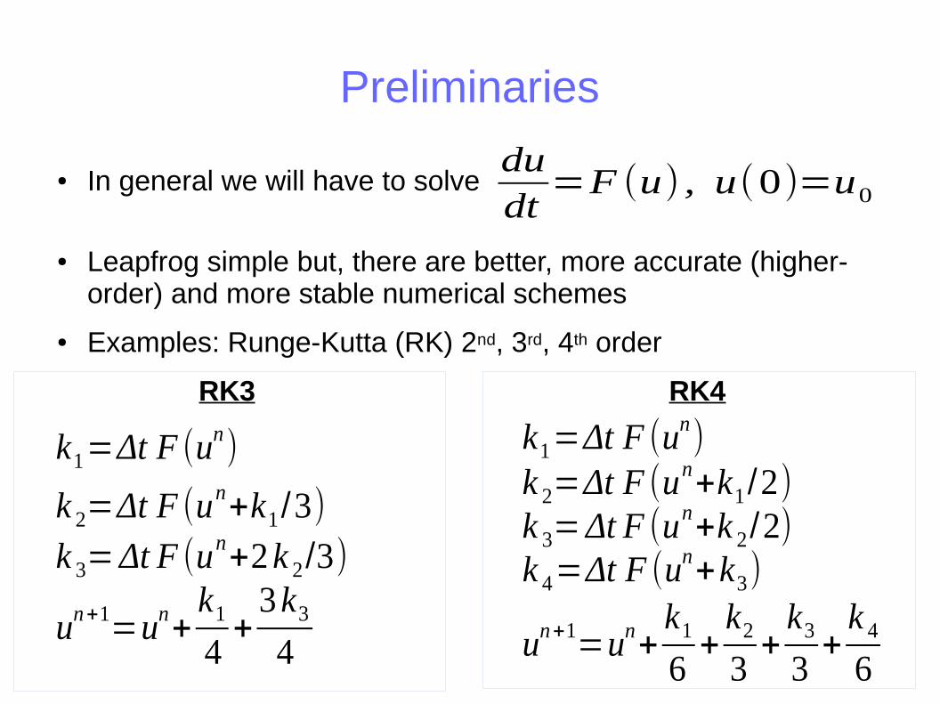
In general we will have to solve
Leapfrog simple but, there are better, more accurate (higher-order) and more stable numerical schemes
Examples: Runge-Kutta (RK) 2nd, 3rd, 4th order
RK3 RK4
dudt
=F (u) , u(0)=u0
un+1=un
+k1
4+
3k3
4
k1=Δt F (un)
k 2=Δt F (un+k1/3)
un+1=un
+k1
6+
k2
3+
k3
3+
k 4
6
k1=Δt F (un)
k 2=Δt F (un+k1/2)
k 3=Δt F (un+k 2/2)
k 4=Δt F (un+k3)
k 3=Δt F (un+2k 2/3)

Preliminaries
Solving the initial value problem for partial differential equations (PDEs)
In general we will have to solve
The concept of the method of lines
– Discretize the spatial derivatives
– Find a numerical approximation to the function
– Treat as a large number of ODEs (one for
each spatial cell) and use your favorite ODE solver.
∂u∂ t
=F(u ,∂i u ,∂i ∂ j u , ...) , u(0,x i)=u0, i=1,2,3
FN F
∂u∂ t
=FN

Why Finite Differencing?
• There are several general approaches to the numerical solution of timedependent PDEs, including
1. Finite differences2. Finite volume3. Finite elements4. Spectral
• Finite difference (FD) methods are particularly appropriate when the solution isexpected to be smooth “(infinitely differentiable“) given that the initial data issmooth
• This is the case for many classical field theories including those for a scalar(linear/nonlinear Klein Gordon), vector (electromagnetism [Maxwell]), rank-2symmetric tensor (general relativity [Einstein])
• In cases where solutions do not remain smooth, even if the initial data is—ashappens in compressible hydrodynamics, for example, where shocks can
7
form -- the finite volume approach is the method of choice (Wednesday)

Why Finite Differencing?
• Accessibility: Requires a minimum of mathematical background: if you’remathematically mature enough to understand the nature of the PDEs you needto solve, you’re mathematically mature enough to understand finite differencing
• Flexibility: Technique can be used for essentially any system of PDEs that hassmooth solutions, irrespective of
• Number of dependent variables (unknown functions)
• Number of independent variables (a.k.a. “dimensionality” of the system:nomenclature “1-D” means dependence on one spatial dimension plus time,“2-D”, “3-D” similarly mean dependence on two/three dimensions, plustime, respectively)
• Nonlinearity
• Form of equations: technique does not require that the system of equationshas any particular/special form (contrast with finite volume methods whereone generally wants to cast the equations in so-called conservation-law form)
8

Why Finite Differencing?
• Error analysis:
• Mathematically rigorous: Quite difficult
• Practical/empirical: Extremely straightforward—basic principle is to computemultiple solutions using same initial data and problem parameters, butdiffering fundamental discretization scales. Comparison of solutions providesdirect estimate of error in solutions
• Adaptivity: Can combine basic method with changes in
• Local scale of discretization
• Order of approximation
in order to maximize increase in solution accuracy as a function ofcomputational work invested (e.g. adaptive mesh refinement, week 3)
• Parallelization: Due to “locality of influence” in finite difference schemes, it isrelatively easy to write FD codes than run efficiently on large distributedmemory computer clusters having 1000s or cores (these days 10,000s or even100,000s!)
9

Why Finite Differencing?
• Sufficiency: FD techniques are often sufficient to generate solutions ofacceptable accuracy, again assuming that solutions are smooth
• Will usually not be the most efficient and/or accurate among possibleapproaches, but when one is looking for a solution for the first time (sciencevs engineering/technology), such considerations are often not very important
• Now proceed to illustration of finite difference technique through the solutionof the simple and familiar 1-D wave equation
10

1. Mathematical Formulation
11

The 1-D Wave Equation
• Consider the following initial value (Cauchy) problem for the scalar functionφ(t, x)
φtt = c2φxx , −∞ ≤ x ≤ ∞ , t ≥ 0 (1)
φ(0, x) = φ0(x) (2)
φt(0, x) = Π0(x) (3)
where c is a positive constant, we have adopted the subscript notation forpartial differentiation, e.g. φtt ≡ ∂2φ/∂t2, and we wish to determine φ(t, x) inthe solution domain from the initial conditions (2–3) and the governingequation (1)
• Note the following:
• Since the spatial domain is unbounded, there are no boundary conditions
• Since the equation is second order in time, two functions-worth of initial datamust be specified: the initial scalar field profile, φ0(x), and the initial timederivative, Π0(x)• This system is well posed, and if the initial conditions φ0(x) and Π0(x) are
smooth—which we will hereafter assume—so is the complete solution φ(t, x)
12

The 1-D Wave Equation
• Eqn. (1) is a hyperbolic PDE, and as such, its solutions generically describe thepropagation of disturbances at some finite speed(s), which in this case is c
• Without loss of generality, we can assume that we have adopted units in whichthis speed satisfies c = 1. Our problem then becomes
φtt = φxx , −∞ ≤ x ≤ ∞ , t ≥ 0 (4)
φ(0, x) = φ0(x) (5)
φt(0, x) = Π0(x) (6)
• In the study of the solutions of hyperbolic PDEs, using either closed form(preferred to “analytic”) or numerical approaches, the concept of characteristicis crucial
• Loosely, in a spacetime diagram, characteristics are the lines/surfaces alongwhich information/signals propagate(s).
13

The 1-D Wave Equation
t
: "left−directed" characteristics, x + t = constant , l(x + t)
: "right−directed" characteristics, x − t = constant , r(x − t)
x
• General solution of (4) is a superposition of an arbitrary left-moving profile(v = −c = −1), and an arbitrary right-moving profile (v = +c = +1); i.e.
φ(t, x) = `(x+ t) + r(x− t) (7)
where
` : constant along “left-directed” characteristics
r : constant along “right-directed” characteristics
14

The 1-D Wave Equation
• Observation provides alternative way of specifying initial values—oftenconvenient in practice
• Rather than specifying u(x, 0) and ut(x, 0) directly, specify initial left-movingand right-moving parts of the solution, `(x) and r(x)
• Specifically, set
φ(x, 0) = `(x) + r(x) (8)
φt(x, 0) = `′(x)− r′(x) ≡ d`
dx(x)− dr
dx(x) (9)
• For illustrative purposes will frequently take profile functions φ0(x), `(x), r(x)to be “gaussians”, e.g.
φ0(x) = A exp[− ((x− x0) /δ)2
](10)
where A, x0 and δ are viewed as adjustable parameters that control the overallsize/height of the profile (A), its centre point (x0) and its effective width (δ)
15

2. Discretization
16

Deriving Finite Difference Formulae
• Essence of finite-difference approximation of a PDE:
• Replacement of the continuum by a discrete lattice of grid points
• Replacement of derivatives/differential operators by finite-differenceexpressions
• Finite-difference expressions (finite-difference quotients) approximate thederivatives of functions at grid points, using the grid values themselves. Alloperators and expressions needed here can easily be worked out using Taylorseries techniques.
• Example: Consider task of approximating the first derivative ux(x) of afunction u(x), given a discrete set of values uj ≡ u(jh)
17
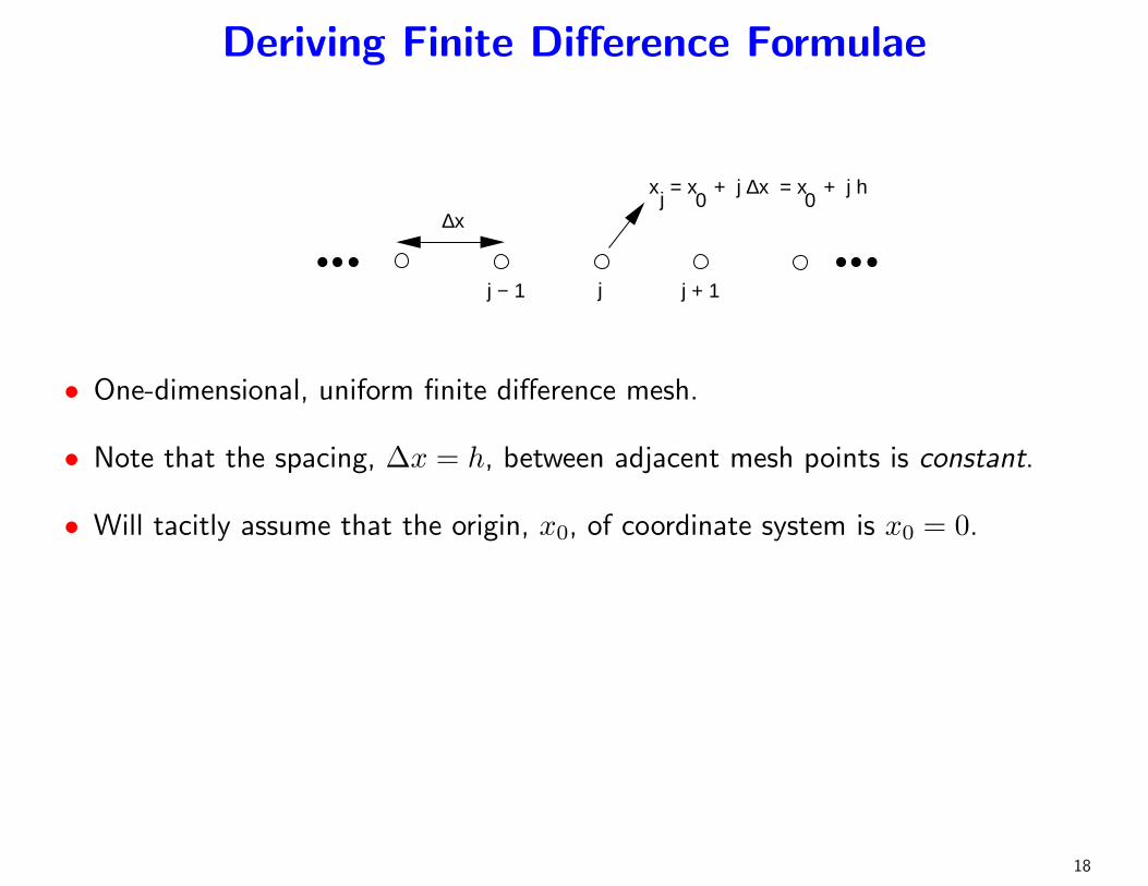
Deriving Finite Difference Formulae
∆x
j − 1 j j + 1
x = x + j ∆x = x + j h j 0 0
• One-dimensional, uniform finite difference mesh.
• Note that the spacing, ∆x = h, between adjacent mesh points is constant.
• Will tacitly assume that the origin, x0, of coordinate system is x0 = 0.
18

Deriving Finite Difference Formulae
• Given the three values u(xj − h), u(xj) and u(xj + h), denoted uj−1, uj, anduj+1 respectively, can compute an O(h2) approximation to ux(xj) ≡ (ux)j asfollows
• Taylor expanding, have
uj−1 = uj − h(ux)j +12h2(uxx)j −
16h3(uxxx)j +
124h4(uxxxx)j +O(h5)
uj = uj
uj+1 = uj + h(ux)j +12h2(uxx)j +
16h3(uxxx)j +
124h4(uxxxx)j +O(h5)
• Now seek a linear combination of uj−1, uj, and uj+1 which yields (ux)j toO(h2) accuracy, i.e. we seek c−, c0 and c+ such that
c− uj−1 + c0 uj + c+ uj+1 = (ux)j +O(h2)
19

Deriving Finite Difference Formulae
• Results in a system of three linear equations for uj−1, uj, and uj+1:
c− + c0 + c+ = 0
−hc− + hc+ = 112h2c− +
12h2c+ = 0
which has the solution
c− = − 12h
c0 = 0
c+ = +1
2h
• Thus, O(h2) FDA (finite difference approximation) for the first derivative is
u(x+ h)− u(x− h)2h
= ux(x) +O(h2) (11)
20

Deriving Finite Difference Formulae
• May not be obvious a priori, that the truncation error of approximation is O(h2)
• Naive consideration of the number of terms in the Taylor series expansionwhich can be eliminated using 2 values (namely u(x+ h) and u(x− h))suggests that the error might be O(h).
• Fact that the O(h) term “drops out” a consequence of the symmetry, orcentering of the stencil: common theme in such FDA, called centred differenceapproximations
• Using same technique, can easily generate O(h2) expression for the secondderivative, which uses the same difference stencil as the above approximationfor the first derivative.
u(x+ h)− 2u(x) + u(x− h)h2
= uxx(x) +O(h2) (12)
• Exercise: Compute the precise form of the O(h2) terms in expressions (11)and (12).
21

Sample FDA for the 1-D Wave Equation
• Let us consider the 1-D wave equation again, but this time on the finite spatialdomain, 0 ≤ x ≤ 1, where we will prescribe fixed (Dirichlet) boundaryconditions
• Then we wish to solve
φtt = φxx (c = 1) 0 ≤ x ≤ 1, t ≥ 0 (13)
φ(0, x) = φ0(x)
φt(0, x) = Π0(x)
φ(t, 0) = φ(t, 1) = 0 (14)
• We will again require that the initial data functions, φ0(x) and Π0(x) besmooth
• Moreover, in order to ensure a smooth solution everywhere, the initial valuesmust be compatible with the boundary conditions, i.e.
φ0(0) = φ0(1) = Π0(0) = Π0(1) = 0 (15)
22

Sample FDA for the 1-D Wave Equation
• As always, we begin the discretization process by replacing the continuumsolution domain with a finite difference mesh, whose typical element(point/event) we will denote by (xj, t
n):
tn ≡ n4t , n = 0, 1, 2, · · ·xj ≡ (j − 1) 4x , j = 1, 2, · · · J
φnj ≡ φ(n4t , (j − 1)4x )
4x = (J − 1)−1
4t = λ4x λ ≡ “Courant number”
• We note in passing that the quantity λ defined above is often called theCourant number or Courant factor, after the great 20th century mathematicianRichard Courant who was a pioneer in the study of finite difference solutions oftime dependent PDEs (in particular, in the use of FD techniques to establishexistence and uniqueness of such PDEs) )
23

Uniform Grid for 1-D Wave Equation
j − 1 j j + 1
∆x
∆t
t
x
• When solving wave equations using FDAs, typically keep λ constant when 4xvaried.
• FDA will always be characterized by the single discretization scale, h.
4x ≡ h
4t ≡ λh
24

FDA for 1-D Wave Equation
• Discretized Interior equation
(4t )−2(φ
n+1j − 2φn
j + φn−1j
)= (φtt)
nj +
1124t 2 (φtttt)
nj +O(4t 4)
= (φtt)nj +O(h2)
(4x )−2(φ
nj+1 − 2φn
j + φnj−1
)= (φxx) n
j +1124x 2 (φxxxx) n
j +O(4x 4)
= (φxx) nj +O(h2)
Putting these two together, get O(h2) approximation
φn+1j − 2φn
j + φn−1j
4t 2=φn
j+1 − 2φnj + φn
j−1
4x 2j = 2, 3, · · · , J − 1 (16)
• Scheme such as (16) often called a three level scheme since couples three “timelevels” of data (i.e. unknowns at three distinct, discrete times tn−1, tn, tn+1.
26

FDA for 1-D Wave Equation
• Discretized Boundary conditions
φn+11 = φ
n+1J = 0
• Discretized Initial conditions
• Need to specify two “time levels” of data (effectively φ(x, 0) and φt(x, 0)),i.e. we must specify
φ0j , j = 1, 2, · · · , J
φ1j , j = 1, 2, · · · , J
ensuring that the initial values are compatible with the boundary conditions.
• Can solve (16) explicitly for φn+1j :
φn+1j = 2φn
j − φn−1j + λ2
(φ
nj+1 − 2φn
j + φn−1j
)(17)
27

Stencil for “Standard” O(h2) Approximation of 1-DWave Equation
n
n + 1
n − 1
j − 1 j j + 1
25

FDA for 1-D Wave Equation
• Also note that (17) is actually a linear system for the unknownsφn+1
j , j = 1, 2, · · · , J ; in combination with the discrete boundary conditionscan write
A φn+1 = b (18)
where A is a diagonal J × J matrix and φn+1 and b are vectors of length J .
• Such a difference scheme for an IVP is called an explicit scheme.
28

FDAs: Back to the Basics—Concepts & Definitions
• Will be considering the finite-difference approximation (FDA) of PDEs-0—willgenerally be interested in the continuum limit, where the mesh spacing, or gridspacing, usually denoted h, tends to 0.
• Because any specific calculation must necessarily be performed at somespecific, finite value of h, we will also be (extremely!) interested in the waythat our discrete solution varies as a function of h.
• Will always view h as the basic “control” parameter of a typical FDA.
• Fundamentally, for sensibly constructed FDAs, we expect the error in theapproximation to go to 0, as h goes to 0.
41

Some Basic Concepts, Definitions and Techniques
• LetLu = f (54)
denote a general differential system.
• For simplicity, concreteness, can think of u = u(x, t) as a single function of onespace variable and time,
• Discussion applies to cases in more independent variables(u(x, y, t), u(x, y, z, t) · · · etc.), as well as multiple dependent variables(u = u = [u1, u2, · · · , un]).
• In (54), L is some differential operator (such as ∂tt− ∂xx) in our wave equationexample), u is the unknown, and f is some specified function (frequently calleda source function) of the independent variables.
42

Some Basic Concepts, Definitions and Techniques
• Here and in the following, will sometimes be convenient use notation where asuperscript h on a symbol indicates that it is discrete, or associated with theFDA, rather than the continuum.
• With this notation, we will generically denote an FDA of (54) by
Lhuh = fh (55)
where uh is the discrete solution, fh is the specified function evaluated on thefinite-difference mesh, and Lh is the finite-difference approximation of L.
43

Residual
• Note that another way of writing our FDA is
Lhuh − fh = 0 (56)
• Often useful to view FDAs in this form for following reasons
• Have a canonical view of what it means to solve the FDA—“drive theleft-hand side to 0”.
• For iterative approaches to the solution of the FDA (which are common,since it may be too expensive to solve the algebraic equations directly), arenaturally lead to the concept of a residual.
• Residual is simply the level of “non-satisfaction” of our FDA (and, indeed, ofany algebraic expression).
• Specifically, if uh is some approximation to the true solution of the FDA, uh,then the residual, rh, associated with uh is just
rh ≡ Lhuh − fh (57)
• Leads to the view of a convergent, iterative process as being one which “drivesthe residual to 0”.
44

Truncation Error
• Truncation error, τh, of an FDA is defined by
τh ≡ Lhu− fh (58)
where u satisfies the continuum PDE (54).
• Note that the form of the truncation error can always be computed (typicallyusing Taylor series) from the finite difference approximation and the differentialequations.
45

Convergence
• Assume FDA is characterized by a single discretization scale, h,
• we say that the approximation converges if and only if
uh → u as h→ 0. (59)
• In practice, convergence is clearly our chief concern as numerical analysts,particularly if there is reason to suspect that the solutions of our PDEs aregood models for real phenomena.
• Note that this is believed to be the case for many interesting problems ingeneral relativistic astrophysics—the two black hole problem being an excellentexample.
46

Consistency
• Assume FDA with truncation error τh is characterized by a single discretizationscale, h,
• Say that the FDA is consistent if
τh → 0 as h→ 0. (60)
• Consistency is obviously a necessary condition for convergence.
47

Order of an FDA
• Assume FDA is characterized by a single discretization scale, h
• Say that the FDA is p-th order accurate or simply p-th order if
limh→0
τh = O(hp) for some integer p (61)
48

Solution Error
• Solution error, eh, associated with an FDA is defined by
eh ≡ u− uh (62)
49

Relation Between Truncation Error and SolutionError
• Common to tacitly assume that
τh = O(hp) −→ eh = O(hp)
• Assumption is often warranted, but is extremely instructive to consider why it iswarranted and to investigate (following Richardson 1910 (!)) in some detail thenature of the solution error.
• Will return to this issue in more detail later.
50

Error Analysis and Convergence Tests
• Discussion here applies to essentially any continuum problem which is solvedusing FDAs on a uniform mesh structure.
• In particular, applies to the treatment of ODEs and elliptic problems
• For such problems convergence is often easier to achieve due to fact that theFDAs are typically intrinsically stable
• Also note that departures from non-uniformity in the mesh do not, in general,complete destroy the picture: however, do tend to distort it in ways that arebeyond the scope of these notes.
• Difficult to overstate importance of convergence studies
51

Richardson Ansatz
Key idea behind error analysis: The Richardson ansatz: Appeal to L.F. Richardson’s old observation (ansatz), that the solution of any FDA which
1. Uses a uniform mesh structure with scale parameter h,
2. Is completely centered
should have the following expansion in the limit h → 0: (72) Here u is the continuum solution, while , , · · · are (continuum) error
functions which do not depend on h. The Richardson expansion (72), is the key expression from which almost
all error analysis of FDAs derives.
uh
uh(x , t )=u (x ,t )+h2 e2(x , t)+h4 e4( x , t) ...
e2 e4

Convergence Tests
• A simple example of a convergence test, and one commonly used in practice isas follows.
• Compute three distinct FD solutions uh, u2h, u4h at resolutions h, 2h and 4hrespectively, but using the same initial data (as naturally expressed on the 3distinct FD meshes).
• Also assume that the finite difference meshes “line up”, i.e. that the 4h gridpoints are a subset of the 2h points which are a subset of the h points
• Thus, the 4h points constitute a common set of events (xj, tn) at which
specific grid function values can be directly (i.e. no interpolation required) andmeaningfully compared to one another.
63

Convergence Tests• From the Richardson ansatz (72), expect:
uh = u+ h2e2 + h4e4 + · · ·u2h = u+ (2h)2e2 + (2h)4e4 + · · ·u4h = u+ (4h)2e2 + (4h)4e4 + · · ·
• Then compute a quantity Q(t), which will call a convergence factor, as follows:
Q(t) ≡ ‖u4h − u2h‖x‖u2h − uh‖x
(78)
where ‖ · ‖x is any suitable discrete spatial norm, such as the `2 norm, ‖ · ‖2:
‖uh‖2 =
J−1J∑
j=1
(uh
j
)21/2
(79)
• Subtractions in (78) can be taken to involve the sets of mesh points which arecommon between u4h and u2h, and between u2h and uh.
64

Convergence Tests
• Is simple to show that, if the FD scheme is converging, then should find:
limh→0
Q(t) = 4. (80)
• In practice, can use additional levels of discretization, 8h, 16h, etc. to extendthis test to look for “trends” in Q(t) and, in short, to convince oneself (and,with luck, others), that the FDA really is converging.
• Additionally, once convergence of an FDA has been established, then point-wisesubtraction of any two solutions computed at different resolutions, immediatelyprovides an estimate of the level of error in both.
• For example, if one has uh and u2h, then, again by the Richardson ansatz have
u2h − uh =((u+ (2h)2e2 + · · ·
)−(u+ h2e2 + · · ·
))(81)
= 3h2e2 +O(h4) ∼ 3eh ∼ 34e2h (82)
65

Richardson Extrapolation
• Richardson extrapolation: Richardson’s observation (72) also provides the basisfor all the techniques of Richardson extrapolation
• Solutions computed at different resolutions are linearly combined so as toeliminate leading order error terms, providing more accurate solutions.
• As an example, given uh and u2h which satisfy (72), can take the linearcombination
uh ≡ 4uh − u2h
3(83)
which, by (72), is easily seen to be O(h4), i.e. fourth-order accurate!
uh ≡ 4uh − u2h
3=
4(u+ h2e2 + h4e4 + · · ·
)−(u+ 4h2e2 + 16h4e4 + · · ·
)3
= −4h4e4 +O(h6) = O(h4) (84)
66
Richardson Extrapolation
• When it works, Richardson extrapolation has an almost magical quality about it
• However, generally have to start with fairly accurate (on the order of a few %)solutions in order to see the dramatic improvement in accuracy suggestedby (84).
• Still a struggle to achieve that sort of accuracy (i.e. a few %) for anycomputation in many areas of numerical relativity/astrophysics and keep theerror smooth (which is necessary for Richardson extrapolation to be effective)
• Thus, techniques based on Richardson extrapolation have not had a majorimpact in this context, although higher-order O(h4), O(h6) etc. finitedifference methods are increasingly common for the vacuum Einstein equations
67

Independent Residual Evaluation
• Question that often arises in convergence testing: is the following:
“OK, you’ve established that uh is converging as h→ 0, but how do youknow you’re converging to u, the solution of the continuum problem?”
• Here, notion of an independent residual evaluation is very useful.
• Idea is as follows: have continuum PDE
Lu− f = 0 (85)
and FDALhuh − fh = 0 (86)
• Assume that uh is apparently converging from, for example, computation ofconvergence factor (78) that looks like it tends to 4 as h tends to 0.
• However, do not know if we have derived and/or implemented our discreteoperator Lh correctly.
68

Independent Residual Evaluation
• Note that implicit in the “implementation” is the fact that, particularly formulti-dimensional and/or implicit and/or multi-component FDAs, considerable“work” (i.e. analysis and coding) may be involved in setting up and solving thealgebraic equations for uh.
• As a check that solution is converging to u, consider a distinct (i.e.independent) discretization of the PDE:
Lhuh − fh = 0 (87)
• Only thing needed from this FDA for the purposes of the independent residualtest is the new FD operator Lh.
• As with Lh, can expand Lh in powers of the mesh spacing:
Lh = L+ h2E2 + h4E4 + · · · (88)
where E2, E4, · · · are higher order (involve higher order derivatives than L)differential operators.
69

Independent Residual Evaluation
• Now simply apply the new operator Lh to our FDA uh and investigate whathappens as h→ 0.
• If uh is converging to the continuum solution, u, will have
uh = u+ h2e2 +O(h4) (89)
and will compute
Lhuh =(L+ h2E2 +O(h4)
) (u+ h2e2 +O(h4)
)(90)
= Lu+ h2(E2 u+ Le2) (91)
= O(h2) (92)
• That is Lhuh will be a residual-like quantity that converges quadratically ash→ 0.
70

Stability Analysis• One of the most frustrating/fascinating features of FD solutions of time
dependent problems: discrete solutions often “blow up”—e.g. floating-pointoverflows are generated at some point in the evolution
• ‘Blow-ups” can sometimes be caused by legitimate (!) “bugs”—i.e. anincorrect implementation—at other times it is simply the nature of the FDscheme which causes problems.
• Are thus lead to consider the stability of solutions of difference equations
• Again consider the 1-d wave equation, utt = uxx
• Note that it is a linear, non-dispersive wave equation
• Thus the “size” of the solution does not change with time:
‖u(x, t)‖ ∼ ‖u(x, 0)‖ , (95)
where ‖ · ‖ is an suitable norm, such as the L2 norm:
‖u(x, t)‖ ≡(∫ 1
0
u(x, t)2 dx)1/2
. (96)
73
Stability Analysis
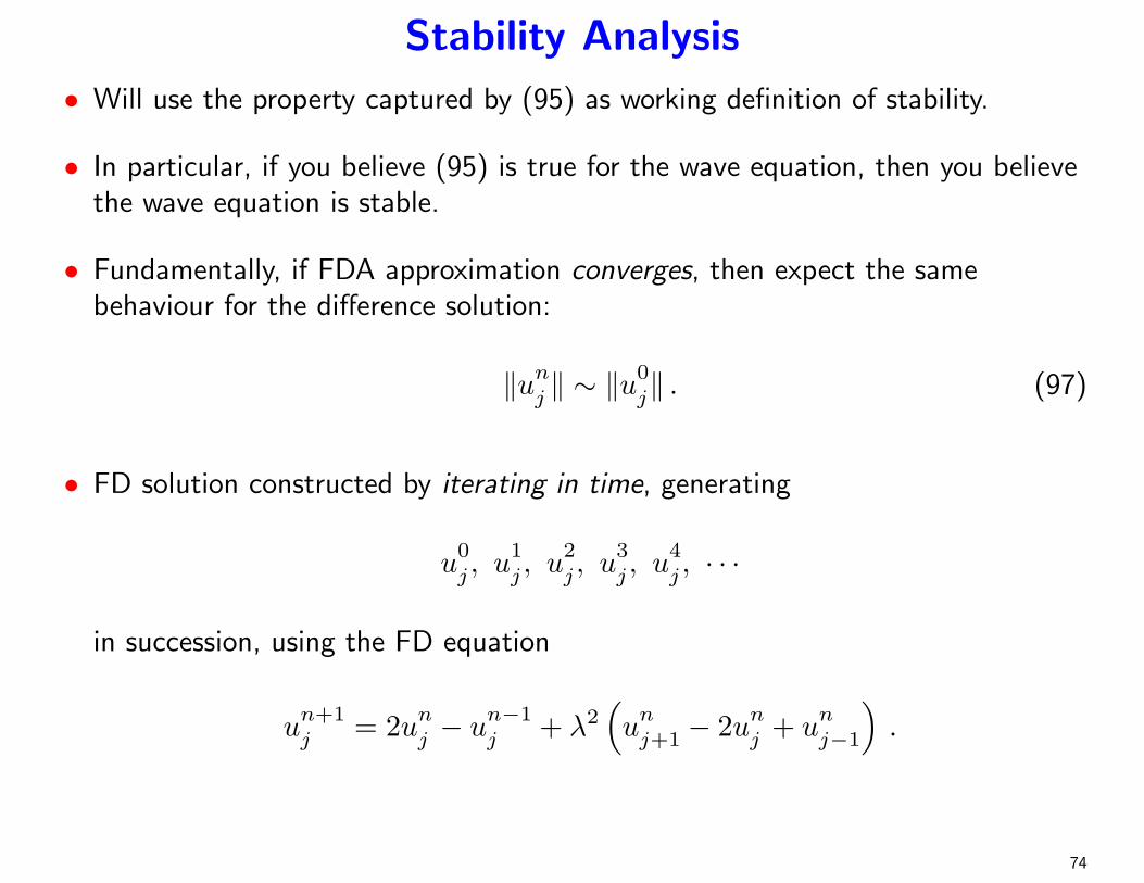
• Will use the property captured by (95) as working definition of stability.
• In particular, if you believe (95) is true for the wave equation, then you believethe wave equation is stable.
• Fundamentally, if FDA approximation converges, then expect the samebehaviour for the difference solution:
‖unj ‖ ∼ ‖u
0j‖ . (97)
• FD solution constructed by iterating in time, generating
u0j , u
1j , u
2j , u
3j , u
4j , · · ·
in succession, using the FD equation
un+1j = 2un
j − un−1j + λ2
(u
nj+1 − 2un
j + unj−1
).
74

Stability Analysis
• Not guaranteed that (97) holds for all values of λ ≡ 4t /4x .
• For certain λ, have‖un
j ‖ ‖u0j‖ ,
and for those λ, ‖un‖ diverges from u, even (especially!) as h→ 0—that is,the difference scheme is unstable.
• For many wave problems (including all linear problems), given that a FDscheme is consistent (i.e. so that τ → 0 as h→ 0), stability is the necessaryand sufficient condition for convergence (Lax’s theorem).
75

Heuristic Stability Analysis
• Write general time-dependent FDA in the form
un+1 = G[un] , (98)
• G is some update operator (linear in our example problem)
• u is a column vector containing sufficient unknowns to write the problem infirst-order-in-time form.
• Example: introduce new, auxiliary set of unknowns, vnj , defined by
vnj = u
n−1j ,
then can rewrite differenced-wave-equation (16) as
un+1j = 2un
j − vnj + λ2
(u
nj+1 − 2un
j + unj−1
), (99)
vn+1j = u
nj , (100)
76

Heuristic Stability Analysis
• Thus withun = [un
1 , vn1 , u
n2 , v
n2 , · · · u
nJ , v
nJ ] ,
(for example), (99-100) is of the form (98).
• Equation (98) provides compact way of describing the FDA solution.
• Given initial data, u0, solution after n time-steps is
un = Gnu0, (101)
where Gn is the n-th power of the matrix G.
• Assume that G has a complete set of orthonormal eigenvectors
ek, k = 1, 2, · · · J ,
and corresponding eigenvalues
µk, k = 1, 2, · · · J ,
77

Heuristic Stability Analysis
• Thus haveGek = µk ek, k = 1, 2, · · · J .
• Can then write initial data as (spectral decomposition):
u0 =J∑
k=1
c0k ek ,
where the c0k are coefficients.
• Using (101), solution at time-step n is
un = Gn
(J∑
k=1
c0k ek
)(102)
=J∑
k=1
c0k (µk)n ek . (103)
78

Heuristic Stability Analysis
• If difference scheme is to be stable, must have
|µk| ≤ 1 k = 1, 2, · · · J (104)
(Note: µk will be complex in general, so |µ| denotes the complex modulus,|µ| ≡
√µµ?).
• Geometric interpretation: eigenvalues of the update matrix must lie on orwithin the unit circle
79

Heuristic Stability AnalysisIm
Re
unit circle
• Schematic illustration of location in complex plane of eigenvalues of updatematrix G.
• In this case, all eigenvalues (dots) lie on or within the unit circle, indicatingthat the corresponding finite difference scheme is stable.
80

Von-Neumann (Fourier) Stability Analysis(Summary)
• Von-Neumann (VN) stability analysis based on the ideas sketched above
• Assumes that difference equation is linear with constant coefficients, periodicboundary conditions boundary conditions are periodic
• Can then use Fourier analysis: difference operators in real-space variable x −→algebraic operations in Fourier-space variable k
• VN applied to wave-equation example shows that must have
λ ≡ 4t4x≤ 1 ,
for stability of scheme (16).
• Condition is often called the CFL condition—after Courant, Friedrichs andLewy who derived it in 1928
• This type of instability has “physical” interpretation, often summarized by thestatement the numerical domain of dependence of an explicit difference schememust contain the physical domain of dependence.
81

1-D Wave Equation: 1st Order Form
• Let us again consider the 1-D wave equation, solved on the spatial domain0 ≤ x ≤ 1, and where we will delay the specification of the boundary conditionsfor the time being
• We have
φtt = φxx , 0 ≤ x ≤ 1 , t ≥ 0 (19)
φ(0, x) = φ0(x) (20)
φt(0, x) = Π0(x) (21)
• We rewrite (19) in a form that involves only first time derivatives by definingthe following auxiliary variables
Φ(t, x) ≡ φx (22)
Π(t, x) ≡ φt (23)
30

1-D Wave Equation: 1st Order Form
• Using the commutativity of (mixed) partial derivatives, it is easy to showthat (19) is equivalent to the following system
Φt = Πx (24)
Πt = Φx (25)
• The initial conditions are then given by
Φ(0, x) =d
dxφ0(x) (26)
Π(0, x) = Π0(x) (27)
• We also note that if we are not concerned with actually computing values ofthe scalar field, φ(t, x) itself (and in this treatment we will not be), then wecan equally well replace (26) with
Φ(0, x) = Φ0(x) (28)
i.e. we can specify the initial values of Φ ≡ φx directly31

1-D Wave Equation: 1st Order Form
• We now return to the issue of boundary conditions: we wish to illustrate a typeof boundary condition which is often imposed when a (pure) initial-valueproblem for a hyperbolic system has been converted into aninitial-boundary-value problem by truncation of the solution domain to somefinite extent
• Thus, although we will solve the wave equation on the spatial domain0 ≤ x ≤ 1, we want the solution to approximate the one that we would get ifwe were able to solve on the unbounded domain −∞ < x <∞
• We assume that the initial conditions represent some set of disturbances whichare localized in space, well away from the boundaries x = 0 and x = 1, andthat the subsequent dynamics describes the propagation of these disturbancesin and away from the interval in which they are initially localized
• We recall that the general solution of the wave equation can be written in theform
φ(t, x) ∼ `(x+ t) + r(x− t) (29)
where ` and r are the left- and right-moving parts of the solution, respectively
32

1-D Wave Equation: 1st Order Form
• We further observe that it follows from (29) and the definitions of Φ and Πthat Φ ≡ φx and Π ≡ φt can also be written as a linear combination of right-and left-moving pieces
• The boundary condition we now wish to employ is often called a radiationcondition, or Sommerfeld condition, and is equivalent to the demand that therebe no incoming radiation (disturbances) at the boundaries of the solutiondomain
• This means that at x = 0 we must have only left-moving signals, so thatΦ(t, x) ∼ Φ(x+ t) and Π(t, x) ∼ Π(x+ t), or
Φt(t, 0) = Φx(t, 0) (30)
Πt(t, 0) = Πx(t, 0) (31)
• Similarly, at x = 1 we require only left-moving waves, so thatΦ(t, x) ∼ Φ(x− t) and Π(t, x) ∼ Π(x− t), or
Φt(t, 1) = −Φx(t, 1) (32)
Πt(t, 1) = −Πx(t, 1) (33)33

1-D Wave Equation: Crank-Nicholson Scheme
• We now discuss the Crank-Nicholson discretization scheme for the 1-D waveequation as written in the first order form defined above: variations on thistheme will be used extensively in this week’s lectures and tutorial sessions
• We adopt the same uniform grid structure (in space and time) as previously,but now use the stencil illustrated on the next page for our PDEs
Φt = Πx
Πt = Φx
• In our description of the Crank Nicholson FDA we will also introduce the notionof finite difference operators, which provide a compact way of denoting manyFDAs, and which play a central role in the special purpose programminglanguage, RNPL, that we will use in the tutorial sessions
34

Stencil for O(h2) Crank-Nicholson Approximation of1-D Wave Equation
j
Scheme is centred at t , xn+1/2
j
j−1 j+1
n
n+1
35

1-D Wave Equation: Crank-Nicholson Scheme
• To illustrate the scheme, it will suffice to consider one of the two first-orderPDEs that together constitute the wave equation: for specificity we focus on
Φt = Πx (34)
• The time derivative of Φ is approximated using
4t−1(
Φn+1j − Φn
j
)= (Φt)
n+12
j +1244t 2 (Φttt)
n+12
j +O(4t 4) (35)
= (Φt)n+1
2j +O(4t 2)
• To approximate Πx, we write the usual O(h2) centred approximation for thefirst derivative in operator form as
Dx Πnj ≡ (24x )−1
(Πn
j+1 −Πnj−1
)(36)
Dx = ∂x +164x 2 ∂xxx +O(4x 4) (37)
36

1-D Wave Equation: Crank-Nicholson Scheme
• We further introduce the (forward) time-averaging operator, µt:
µt unj ≡ 1
2
(u
n+1j + u
nj
)= u
n+12
j +184t 2 (utt)
n+12
j +O(4t 4) (38)
µt =[I +
184t 2 ∂tt +O(4t 4)
]t=tn+1/2
(39)
where I is the identity operator.
• Assuming that 4t = O(4x ) = O(h), it is easy to show (exercise) that
µt
[Dx Πn
j
]= (Πx) n+1
2j +O(h2)
• Putting above results together, we get the (O(h2)) Crank-Nicholsonapproximation of Φt = Πx
Φn+1j − Φn
j
4t= µt
[Dx Πn
j
](40)
37

1-D Wave Equation: Crank-Nicholson Scheme
• Written out in full, this is
Φn+1j − Φn
j
4t=
12
[Πn+1
j+1 −Πn+1j−1
24x+
Πnj+1 −Πn
j−1
24x
](41)
• Note that the Crank-Nicholson scheme immediately generalizes to any equationthat can be written in the form
ut = L[u] (42)
where is L is some spatial operator. A Crank-Nicholson FDA of (42) is
un+1j − un
j
4t=
12(Lh[un+1
]+ Lh [un]
)(43)
where Lh is some discretization of L, not necessarily second order
• Also observe that Crank-Nicholson scheme is a two-level method (couplesunknowns at two discrete time steps)
38

1-D Wave Equation: Crank-Nicholson Scheme
• The difference equations (40) can be applied at grid points labelled byj = 2, 3, . . . , J − 1 (the interior points)
• For j = 1 and j = J we use discretized versions of the radiation (Sommerfeld)boundary conditions
Φt(t, 0) = Φx(t, 0) (44)
Φt(t, 1) = −Φx(t, 1) (45)
• The time derivatives are approximated as previously, and for the spacederivatives we use second order, forward and backward (“off-centred”)difference approximations defined by
DFx Φn
j ≡ (24x )−1(−3Φn
j + 4Φnj+1 − Φn
j+2
)(46)
DFx = ∂x +O(4x 2) exercise (47)
DBx Φn
j ≡ (24x )−1(
3Φnj − 4Φn
j−1 + Φnj−2
)(48)
DBx = ∂x +O(4x 2) exercise (49)
39

1-D Wave Equation: Crank-Nicholson Scheme
• Employing the time-averaging operator, µt, defined previously, the FDAs for theoutgoing-radiation boundary conditions are
Φn+1j − Φn
j
4t= µt
[DF
x Φnj
]j = 1 (50)
Φn+1j − Φn
j
4t= −µt
[DB
x Φnj
]j = J (51)
• Finally, in our RNPL implementation of this scheme, we will set initial data ofthe form
Φ0j = A exp
[− ((x− x0) /δ)2
](52)
Π0j = σΦ0
j (53)
where σ = −1, 0, 1 will generate purely left-moving, left-moving/right-moving(time symmetric) or purely right-moving data, respectively, and where A, x0
and δ are adjustable parameters of the gaussian pulse shape
40