a feynman integral via higher normal functions · a feynman integral via higher normal functions by...

A FEYNMAN INTEGRAL VIA HIGHERNORMAL FUNCTIONS

by

Spencer Bloch, Matt Kerr & Pierre Vanhove

Abstract. —We study the Feynman integral for the three-banana graph defined

as the scalar two-point self-energy at three-loop order. The Feynmanintegral is evaluated for all identical internal masses in two space-timedimensions. Two calculations are given for the Feynman integral; onebased on an interpretation of the integral as an inhomogeneous solu-tion of a classical Picard-Fuchs differential equation, and the other usingarithmetic algebraic geometry, motivic cohomology, and Eisenstein se-ries. Both methods use the rather special fact that the Feynman integralis a family of regulator periods associated to a family of K3 surfaces. Weshow that the integral is given by a sum of elliptic trilogarithms evalu-ated at sixth roots of unity. This elliptic trilogarithm value is related tothe regulator of a class in the motivic cohomology of the K3 family. Weprove a conjecture by David Broadhurst that at a special kinematicalpoint the Feynman integral is given by a critical value of the Hasse-WeilL-function of the K3 surface. This result is shown to be a particular caseof Deligne’s conjectures relating values of L-functions inside the criticalstrip to periods.

IPHT-T/14/015, IHES/P/14/06.

arX

iv:1

406.

2664

v3 [

hep-

th]

26

Mar

201

5

2 S. BLOCH, M. KERR & P. VANHOVE

Contents

1. Introduction . . . . . . . . . . . . . . . . . . . . . . . . . . . . . . . . . . . . . . . . 3Acknowledgements . . . . . . . . . . . . . . . . . . . . . . . . . . . . . . . . . . . . 62. The three-banana Feynman integral . . . . . . . . . . . . . . . . 6

2.1. The integral . . . . . . . . . . . . . . . . . . . . . . . . . . . . . . . . . . 62.2. The Picard-Fuchs equation . . . . . . . . . . . . . . . . . . 92.3. Solution of the inhomogeneous Picard-Fuchs equation

. . . . . . . . . . . . . . . . . . . . . . . . . . . . . . . . . . . . . . . . . . . . . . 112.4. Value of the integral at t = 0 . . . . . . . . . . . . . . . . 182.5. Value of the integral at t = 1 . . . . . . . . . . . . . . . . 21

3. The family of K3 surfaces . . . . . . . . . . . . . . . . . . . . . . . . . . 233.1. Sunset in a nutshell . . . . . . . . . . . . . . . . . . . . . . . . . . 243.2. Verrill’s family . . . . . . . . . . . . . . . . . . . . . . . . . . . . . . . . 253.3. Miscellany . . . . . . . . . . . . . . . . . . . . . . . . . . . . . . . . . . . . 30

4. The three-banana integral as a higher normal function. . . . . . . . . . . . . . . . . . . . . . . . . . . . . . . . . . . . . . . . . . 32

4.1. K3 of a K3! . . . . . . . . . . . . . . . . . . . . . . . . . . . . . . . . . . 334.2. Review of Abel-Jacobi . . . . . . . . . . . . . . . . . . . . . . . . 364.3. Reinterpreting the Feynman integral . . . . . . . . . . 40

5. A second computation of the three-banana integral: theEisenstein symbol . . . . . . . . . . . . . . . . . . . . . . . . 44

5.1. Higher normal functions of Eisenstein symbols. . . . . . . . . . . . . . . . . . . . . . . . . . . . . . . . . . . . . . . . . . . . . . 44

5.2. Modular pullback of the three-banana cycle . . 505.3. The main result . . . . . . . . . . . . . . . . . . . . . . . . . . . . . . 53

6. Foundational Results via Hodge Theory . . . . . . . . . . . . 546.1. Some lemmas . . . . . . . . . . . . . . . . . . . . . . . . . . . . . . . . 546.2. Applications: CY periods . . . . . . . . . . . . . . . . . . . . 57

7. Special values of the integral . . . . . . . . . . . . . . . . . . . . . . . . 617.1. Special value at t = 1 . . . . . . . . . . . . . . . . . . . . . . . . 617.2. Special value at t = 0 . . . . . . . . . . . . . . . . . . . . . . . . 65

Appendix A. Higher symmetric powers of the sunset motive. . . . . . . . . . . . . . . . . . . . . . . . . . . . . . . . . . . . . . . . . . 67

References . . . . . . . . . . . . . . . . . . . . . . . . . . . . . . . . . . . . . . . . . . . . 68

A FEYNMAN INTEGRAL VIA HIGHER NORMAL FUNCTIONS 3

1. Introduction

The computation of scattering amplitudes in quantum field theory re-quires the evaluation of Feynman integrals. This is a non-trivial taskfor which many techniques have been developed by physicists over theyears (cf. the reviews [BDK, Bri, EKMZ, EH].) Feynman integralsare multivalued functions of the physical parameters, given by the ex-ternal momenta and internal masses. Differentiating with respect to thephysical parameters leads to a first order system of differential equa-tions as in e.g. [H, CHH] or to higher order differential equations as ine.g. [LR, MSWZ, MSWZ2, Va, ABW, ABW2].

The Feynman integral associated to a graph Γ with n edges (propa-gators) is an integral over the positive simplex ∆n := [x1 : · · · : xn] ∈Pn−1(R) |xi ≥ 0 in projective (n−1)-space of a meromorphic differential(n− 1)-form:

(1.1) IΓ =ˆ

∆n

ΩΓ .

The form ΩΓ depends on the physical parameters – that is, the externalmomenta and internal masses attached to the graph – and is expressedin terms of the first and second Symanzik polynomial [IZ]. The variablesxi are the Schwinger proper times indexed by edges (propagators).

For the algebro-geometric approach of [BEK], the Feynman integralIΓ is a period of the mixed Hodge structure on the relative cohomologygroup Hn−1(Pn−1\XΓ, B\(B ∩XΓ)), where XΓ is the graph hypersurfacedefined by the poles of ΩΓ and B is a blow-up of the simplex ∆n. Varyingthe physical parameters leads to a variation of the Hodge structure. As aresult, the Feynman integral satisfies a set of first order differential equa-tions under the action of the the Gauss-Manin connection [G], leadingto an inhomogeneous Picard-Fuchs equation. The inhomogeneous termhas its origin in the extension of mixed Hodge structure associated withFeynman graphs. The dependence on external momenta means that we


have a family of extensions, also known as a normal function from thework of Poincaré [P] and Griffiths [G2].

This point of view enables us to bring to bear a number of techniquesincluding Picard-Fuchs differential equations, motivic cohomology andregulators, Eisenstein series, and Hodge structures, for the analysis ofthe properties of Feynman integrals.

The main topic of this paper is the evaluation of the Feynman integralfor the three-banana graph

(1.2) IQ(t) :=ˆx1,x2,x3≥0

1(1 +∑3

i=1 xi)(1 +∑3i=1 x

−1i )− t

3∏i=1

dxixi

.

The associated graph hypersurfaceXQ(t) := (1+∑3i=1 xi)(1+∑3

i=1 x−1i )−

t = 0 leads to a family of K3 surfaces with (generic) Picard number 19,over the modular curve P1 \ 0, 4, 16,∞ ∼= Y1(6)+3. It is closely relatedto the family of elliptic curves over Y1(6), which was studied in [BV] inconnection with the Feynman integral arising from the sunset (two-loopbanana) graph.

We prove in theorems 2.3.2 and 5.3.1 that the Feynman integral eval-uates to the product of a period $1(τ) of the K3 surface and an Eichlerintegral of an Eisenstein series. Explicitly, we have

(1.3) IQ(t) = $1(τ)∑n≥1

ψ(n)n3

qn

1− qn − 4(log q)3 + 16ζ(3) ,

where q = exp(2πiτ), ψ(n) is a mod-6 character given in eq. (2.3.24),and t is related to τ by the Hauptmodul (2.3.11) for Γ1(6)+3.

Remarkably, the Eichler integral factor can be expressed as a combi-nation of the Beilinson-Levin elliptic trilogarithms [BL, L, Z]

(1.4) IQ(t) = $1(τ)(

40π2 log q + 24Li3(τ, ζ6) + 21Li3(τ, ζ26 )

+ 8Li3(τ, ζ36 ) + 7Li3(τ, 1)

)


where ζ6 := exp(iπ/3) is the same sixth root of unity that enters theexpression of the sunset integral studied in [BV].

It turns out that the three-banana integral is associated to a generalizednormal function arising from a family of “higher” algebraic cycles or mo-tivic cohomology classes [KL, DK]. The passage from classical normalfunctions associated to families of cycles to normal functions associated tomotivic classes suggests interesting new links between mathematics andphysics (op.cit.). Actually motivic normal functions can, in many cases,be associated with multiple-valued holomorphic functions which arise asamplitudes as in this work or in the context of open mirror symmetry asin [MW] for instance.

The plan of the paper is the following. In section 2 we derive the inho-mogeneous Picard-Fuchs equation satisfied by the three-banana integral.The solution of the differential equation in terms of the elliptic triloga-rithm is given in theorem 2.3.2. In section 3 we give a construction ofthe family of K3 surfaces associated with the three-banana graph.

In section 4 we show that the three-banana integral IQ(t) is an highernormal function, originating from a family of elements in K3(K3′s) (acharming sort of mathematical eponym). Specifically, we show that theMilnor symbols −x1,−x2,−x3 ∈ KM

3

(C(XQ(t))

)extend to classes

Ξt ∈ H3M(XQ(t),Q(3)). We construct a family of closed 2-currents Rt

representing the Abel-Jacobi classes AJ(Ξt) ∈ H2(XQ(t),C/Q(3)), anda family of holomorphic forms ωt ∈ Ω2(XQ(t)), such that

IQ(t) =ˆXQ(t)

Rt ∧ ωt

(Theorem 4.3.2). This has immediate consequences, including a concep-tual proof of the inhomogeneous Picard-Fuchs equation for IQ(t) (Corol-lary 4.3.3).

In section 5 we pull the higher cycle Ξt back from the family of K3surfaces to a modular Kuga 3-fold, where we are able to recognize it


as an Eisenstein symbol in the sense of Beilinson. Applying a generalcomputation (Theorem 5.1.1ff) of higher normal functions associated toBeilinson’s cycles, gives a “motivic” proof (Theorem 5.3.1) that the three-banana integral IQ(t) takes the form claimed in (1.3)-(1.4). In section 6we give the abstract Hodge-theoretic formulation of the Feynman integralin our case.

Finally, in sections 2.4 and theorem 7.2.1 we show that the integralat t = 0 takes the value IQ(0) = 7ζ(3) recovering at result of [BBDG,Broad1, Broad2]. And in sections 2.5 and 7.1.1 we evaluate the three-banana at the special value t = 1. (The results in section 7 again makecrucial use of Theorem 4.3.2.) We show the regulator to be trivial, whichmeans that the Feynman integral is actually a classical rational period oftheK3 up to a factor of 12πi/

√−15. A conjecture of Deligne then relates

the Feynman integral to the critical value of the Hasse-Weil L-functionof the K3 at s = 2. This proves a result first obtained numerically byBroadhurst in [Broad1, Broad2] up to a rational coefficient.

Acknowledgements

We thank A. Clingher and C. Doran for helpful discussions. We thankDavid Broadhurst for many helpful comments and encouragements. MKthanks the IHÉS for support and good working conditions while part ofthis paper was written. We acknowledge support from the ANR grantreference QST ANR 12 BS05 003 01, and the PICS 6076, and partialsupport from NSF Grant DMS-1068974.

2. The three-banana Feynman integral

2.1. The integral. — We look at the three-loop banana graph in twospace-time dimensions associated with the Feynman graph in figure 2.1.1


Figure 2.1.1. The three-loop three-banana Feynman graph.K is the external momentum in R2 andmi ≥ 0 with i = 1, . . . , 4are internal masses.

(2.1.1) IQ(m1,m2,m3,m4;K) :=ˆR8

δ(∑4i=1 `i +K)∏4

i=1 d2`i∏4

i=1(`2i +m2

i ).

Setting t = K2, this integral can be equivalently represented as (see forinstance [Va, section 8])

(2.1.2) IQ(mi; t) =ˆxi≥0

1(m2

4 +∑3i=1m

2ixi)(1 +∑3

i=1 x−1i )− t

3∏i=1

dxixi

Theorem 2.1.1. — The integral IQ(mi; t) defined in eq (2.1.2) has thefollowing integral representation for t < (∑4

i=1mi)2

(2.1.3) IQ(mi; t) = 23ˆ ∞

0x I0(√tx)

4∏i=1

K0(mix) dx .

The Bessel functions K0, I0 are defined by

(2.1.4) K0(2√ab) := 1

2

ˆ ∞0

e−ax−bxdx

x; for a, b > 0 ,

and

(2.1.5) I0(x) :=∑k≥0

(x

2

)2k 1Γ(k + 1)2 .

For the all equal mass case this Bessel representation has already beengiven in [BBDG, Broad2].


Proof. — For t < (∑4i=1mi)3 we can perform the series expansion

(2.1.6) IQ(mi; t) =∑k≥0

tkIk

with

(2.1.7) Ik :=ˆxi≥0

1(m2

4 +∑3i=1m

2ixi)k+1(1 +∑3

i=1 x−1i )k+1

3∏i=1

dxixi

Exponentiating the denominators using´∞

0 dxxk exp(−ax) = Γ(k+1)/ak+1

for a > 0 we have

(2.1.8)

Ik = 1Γ(k + 1)2

ˆxi≥0

ˆu,v≥0

e−u(1+∑3

i=1 x−1i )−v(m2

4+∑3

i=1m2i xi)

dudv

(uv)−k3∏i=1

dxixi

.

Using the definition in (2.1.4) the integral over each xi leads to a K0(x)Bessel function, therefore

(2.1.9) Ik = 23

Γ(k + 1)2

ˆu,v≥0

e−u−vm24

3∏i=1

K0(2√uvmi)

dudv

(uv)−k .

Changing variables (u, v)→ (x = 2√uv, v) then

Ik = 24

Γ(k + 1)2

ˆv,x≥0

e−x24v−vm

24

3∏i=1

K0(2√uvmi)

(x

2

)2k+2 dxdv

xv

= 25

Γ(k + 1)2

ˆ +∞

0

4∏i=1

K0(mix)(x

2

)2k+2 dx

x(2.1.10)

Now we can perform the summation over k using the series expansion ofthe Bessel function I0(

√t x) given in (2.1.5) to conclude the proof.

For the all equal masses case m1 = m2 = m3 = m4 = 1 we have

IQ(t) :=ˆxi≥0

1(1 +∑3

i=1 xi)(1 +∑3i=1 x

−1i )− t

3∏i=1

dxixi

= 23ˆ ∞

0xI0(√t x)K0(x)4 dx .(2.1.11)


2.2. The Picard-Fuchs equation. — In this section we show thethree-loop banana integral IQ(t) satisfies an inhomogeneous Picard-Fuchsequation given in [MSWZ2, Va], following the derivation given in [Va]for the equal masses banana graphs at all loop orders.

Theorem 2.2.1. — The three-loop banana integral

(2.2.1) IQ(t) =ˆxi≥0

1(1 +∑3

i=1 xi)(1 +∑3i=1 x

−1i )− t

3∏i=1

dxixi

satisfies the inhomogeneous Picard-Fuchs equation L3t IQ(t) = −24 with

the Picard-Fuchs operator L3t given by

(2.2.2)

L3t := t2(t−4)(t−16) d

3

dt3+6t(t2−15t+32) d

2

dt2+(7t2−68t+64) d

dt+t− 4 .

This Picard-Fuchs operator already appeared in the work by Verrillin [Ve] and [MSWZ]. We will comment on the relation to this work in§3.2.

Proof. — We consider the Bessel integral representation of the previoussection

(2.2.3) IQ(t) =∑k≥0

tkIk

where Ik is given by (2.1.10) with m1 = m2 = m3 = m4 = 1

(2.2.4) Ik = 24

Γ(k + 1)2

ˆ +∞

0

(x

2

)2k+1K0(x)4 dx .

Then the action of the Picard-Fuchs operators on this series expansiongives

(2.2.5) L3t IQ(t) =

∑k≥0

(tαk + βk + γk

t

)tkIk

therefore

(2.2.6) L3t IQ(t) = γ0I0

t+γ1I1 + β0I0+

∑k≥1

(αkIk+βk+1Ik+1+γk+2Ik+2) tk


Using the result of the lemma 2.2.2 below, we have L3t IQ(t) = γ1I1+β0I0.

Evaluating the integrals gives that γ1I1 + β0I0 = −24, which proves thetheorem.

Lemma 2.2.2. — The Bessel moment integrals

(2.2.7) Ik = 24

Γ(k + 1)2

ˆ +∞

0

(x

2

)2k+1K0(x)4 dx

satisfy the recursion relation

(2.2.8) αkIk + βk+1Ik+1 + γk+2Ik+2 = 0, k ≥ 0

with for k ≥ 0

αk := (k + 1)3

βk := −2(2k + 1) (5k2 + 5k + 2)(2.2.9)

γk := 64k3 .

Proof. — The proof has been given in [BS, Example 6] (see [O] forrelated considerations). Following this reference we introduce the Besselmoment integrals c4,2k+1 = 22k−3Γ(k + 1)2 Ik. One notices that K0(x)4

satisfies the differential equation L5K0(x)4 = 0 where(2.2.10)

L5 :=(xd

dx

)5

−20x2(xd

dx

)3

−60x2(xd

dx

)2

+8x2(8x2−9)(xd

dx

)+32x2(4x2−1) .

And finally one notices the identities

(2.2.11)ˆ +∞

0xk+j

(xd

dx

)m (K0(x)4

)dx = (−1− k − j)m c4,k+j .

Therefore integrating term by term the expression

(2.2.12)ˆ +∞

0t2k+1 L5K0(x)4 dx = 0

leads to the recursion (2.2.8).


2.3. Solution of the inhomogeneous Picard-Fuchs equation. —We need an intermediate result expressing the solution of the third orderdifferential equation using the Wronskian method. Recall the Wronskianof a linear differential equation

(2.3.1) fn(x)y(x)(n) + . . .+ f1(x)y′ + f0(x)y = 0

is the determinant W (x) := det(y(i)j ) where y1, . . . , yn are independent

solutions. Viewing the equation (2.3.1) as a system of n first order equa-tions, the Wronskian is the solution of the first order equation given bythe determinant of the system. This yields the formula

(2.3.2) W (t) = exp(−ˆ t

fn−1(x)/fn(x) dx).

Consider the inhomogeneous differential equation

(2.3.3) f3(x)y′′′(x) + f2(x)y′′(x) + f1(x)y′(x) + f0(x)y(x) = S(x)

Let yi(x) with i = 1, 2, 3 be three independent solutions of the homoge-neous equation. Let

(2.3.4) W (t) =

∣∣∣∣∣∣∣∣y1(t) y2(t) y3(t)y′1(t) y′2(t) y′3(t)y′′1(t) y′′2(t) y′′3(t)

∣∣∣∣∣∣∣∣be the Wronskian of these solutions, and introduce the modified Wron-skian

(2.3.5) W (t, x) =

∣∣∣∣∣∣∣∣y1(x) y2(x) y3(x)y′1(x) y′2(x) y′3(x)y1(t) y2(t) y3(t)

∣∣∣∣∣∣∣∣ .We have the following identities

W (t, t) = 0; ∂W (t, x)∂t

|x=t = 0; ∂2W (t, x)∂t2

|x=t = W (t)(2.3.6)3∑i=0

fi(t)∂i

∂tiW (t, x) = 0(2.3.7)


A simple computation now yields the general solution for the inhomoge-neous equation (2.3.3)

(2.3.8) y(t) =3∑i=1

αi yi(t) +ˆ t

0W (t, x) S(x) dx

W (x)f3(x) .

For the three-banana graph, the Picard-Fuchs operators in (2.2.2) hasf3(x) = x2(x − 4)(x − 16) and f2(x) = 6x(x2 − 15x + 32) = 3

2df3(x)dx

,therefore the Wronskian is given by

(2.3.9) W (t) = exp(−ˆ t f2(x)

f3(x) dx)

= W0

(t2(t− 4)(t− 16)) 32.

The arbitrary normalizationW0 of theWronskian is be determined in (2.3.18).We now use the fact showed in [Ve, theorem 3], and reviewed in §3.2,that Picard-Fuchs operator is a symmetric square of the sunset Picard-Fuch operator. For t ∈ P1\0, 4, 16,∞ the solutions of the homogenousequations are given by

(2.3.10) (y1(t), y2(t), y3(t)) = $1(τ) (1, 2πiτ, (2πiτ)2) .

In this expression $1(τ) is a period and τ is the period ratio. Theparameter t is the Hauptmodul given by [Ve]

(2.3.11) t(τ) = HQ([τ ]) = −(η(τ)η(3τ)η(2τ)η(6τ)

)6

.

We recall that the Dedekind eta function η(τ) is defined by

(2.3.12) η(τ) = exp(πiτ/12)∞∏n=1

(1− exp(2πinτ))

The special values of the Hauptmodul t = 0, 4, 16,+∞ are obtainedfor the values of τ = 0, −3+i

√3

12 , 3+i√

36 ,+i∞. The nature of the fibers

for these values of the Hauptmodul are discussed in §3.2. The value t = 4is the pseudo-threshold of the Feynman integral and the value t = 16 isthe normal threshold of the Feynman integral.


In the neighborhood |t| > 16 of t =∞ the holomorphic period is givenby

$1(τ) = 1(2πi)3

ˆ|x1|=|x2|=|x3|=1

1(1 +∑3

i=1 xi)(1 +∑3i=1 x

−1i )− t

3∏i=1

dxixi

= −∑n≥0

t−n−1 1(2πi)3

ˆ|x1|=|x2|=|x3|=1

(1 +3∑i=1

xi)n(1 +3∑i=1

x−1i )n

3∏i=1

dxixi

= −∑n≥0

t−n−1 ∑p+q+r+s=n

(n!

p!q!r!s!

)2

.(2.3.13)

Using the above expression for the Hauptmodul t, the period is expressedas

(2.3.14) $1(τ) := (η(2τ)η(6τ))4

(η(τ)η(3τ))2 .

Expanding the modified Wronskian

W (t, x) = y1(t)W23(x)− y2(t)W13(x) + y3(t)W12(x)= $1 (W23(x)− τ(t)W13(x) + τ(t)2W12(x)) .(2.3.15)

and then evaluating yields(2.3.16)W12(t) = 2πi$2

1dτ

dt, W13(t) = (2πi)2$2

1 2τ dτdt, W23(t) = (2πi)3$2

1 τ2 dτ

dt.

Thus

(2.3.17) W (t, x) = (2πi)3$1(τ)$1(x)2 (τ(x)− τ(t))2 dτ

dx.

The condition

(2.3.18) ∂2t W (t, x)

∣∣∣∣x=t

= W (t)

determines the normalization W0 = 2 of the Wronskian.


Therefore the tree-loop banana integral is given by

(2.3.19)

IQ(t) = Iperiod−12(2πi)3$1(t)ˆ t

0(τ(x)− τ(t))2 (x2(x−4)(x−16)) 1

2dτ(x)dx

dx .

where Iperiod is an homogeneous solution belonging to $1(τ)(C + τC +τ 2C).

Lemma 2.3.1. — Using the expressions for the Hauptmodul t and theperiod $1 then the function σ(τ) := −24$1(τ)2 (t(τ)2(t(τ) − 4)(t(τ) −16)) 1

2 has the following representation

(2.3.20) σ(τ) = 15 (−E4(τ) + 16E4(2τ) + 9E4(3τ)− 144E4(6τ))

where E4(τ) is the Eisenstein series

(2.3.21) E4(τ) = 12ζ(4)

∑(m,n) 6=(0,0)

1(mτ + n)4 = 1 + 240

∑n≥1

n3 qn

1− qn

With q := exp(2πiτ) the coefficients σn of the q-expansion

(2.3.22) σ(τ) =∑n≥0

σn qn

are given by σ0 = −24 and

σn = n3 ∑m|n

1m3 ψ(m)(2.3.23)

where ψ(n+ 6) = ψ(n) is an even mod 6 character taking the values

ψ(1) = −48, ψ(2) = 720, ψ(3) = 384,ψ(4) = 720, ψ(5) = −48, ψ(6) = −5760 .(2.3.24)

Proof. — The expression in (2.3.20) is obtained by performing a q expan-sion and verifying that the coefficients are the same to very high-orderin the q-expansion using [Sage].


The expression for the Fourier coefficients in (2.3.23) are easily ob-tained by using that

(2.3.25) E4(τ) = 1 + 240∑n≥1

σ3(n)qn

where σ3(n) = ∑m|nm

3 is the divisor sum, and a reorganization of theq-expansion mod 6.

Recall the polylogarithm functions Lir(z) := ∑∞n=1

zn

nr.

Theorem 2.3.2. — The integral IQ(t) in (2.1.11) with t given in (2.3.11),is given by the following function of q

(2.3.26) IQ(t(τ)) = $1(τ)16ζ(3) +

∑n≥1

ψ(n)n3

qn

1− qn − 4(log q)3

.

with $1(τ) the period in (2.3.14) and ψ the even mod 6 character with thevalues given in (2.3.24). This integral can be expressed as linear combina-tion of the elliptic trilogarithms introduced by Beilinson and Levin [BL,L, Z].

(2.3.27) IQ(t(τ)) = $1(τ)(40π2 log q − 48HQ(τ))

where

(2.3.28) HQ(τ) := 24Li3(τ, ζ6) + 21Li3(τ, ζ26 ) + 8Li3(τ, ζ3

6 ) + 7Li3(τ, 1)

with Li3(τ, z) defined by

(2.3.29) Li3(τ, z) := Li3 (z) +∑n≥1

(Li3 (qnz) + Li3(qnz−1

))

−(− 1

12(log z)3 + 124 log q (log z)2 − 1

720(log q)3).

Proof. — In order to prove the theorem we just evaluate the integralin (2.3.19). We perform the change of variables 2πiτ(t) = log q and


2πiτ(x) = log q to get

(2.3.30) IQ(t) = Iperiod + 12 $1(t)

ˆ q

1

(log q

q

)2

σ(q) d log q .

(Here we used that t = 0 for τ = 0, and Iperiod is a solution of thehomogenous Picard-Fuchs equation in $1(τ)(C+ τ C+ τ 2 C).) The formof the homogenous solution is determined in (2.3.43).

Using the q-expansion for σ(τ) and the following integralsˆ q

1

(log q

q

)2

qnd log q = 2(qn − 1)− 2n log q − n2(log q)2

n3ˆ q

1log

(q

q

)2

d log q = (log q)3

3 .(2.3.31)

Summing all the terms we find that

(2.3.32) IQ(t(τ)) = Iperiod

+$1(τ)σ0

6 (log q)3 +∑n≥1

σnn3

(qn − 1

2 (1 + log(qn))2) .

This leads to

(2.3.33) IQ(t(τ)) = Iperiod + σ0

6 $1(τ)(log q)3 + $1(t)∑n≥1

σnn3 q

n .

We remark that the coefficients σn in (2.3.23) can be expressed in termof the sixth root of unity ζ6 = exp(iπ/3)

(2.3.34) σn = −48n3

6∑r=1

cr∑m|n

1m3 ζ

rm6

n ≥ 1

with cr = 24, 21, 16, 21, 24, 14. This allows to express the q-expansion

(2.3.35) σ0

6 (log q)3 +∑n≥1

σnn3 q

n = −48HQ(τ) + 40π2 log q − 16ζ(3)

where

(2.3.36) HQ(τ) := 24Li3(τ, ζ6) + 21Li3(τ, ζ26 ) + 8Li3(τ, ζ3

6 ) + 7Li3(τ, 1)


is given in terms of the elliptic trilogarithms Li3(τ, z) of Beilinson andLevin [BL, L] defined by

(2.3.37) Li3(τ, z) := Li3 (z) +∑n≥1

(Li3 (qnz) + Li3(qnz−1

))

−(− 1

12(log z)3 + 124 log q (log z)2 − 1

720(log q)3).

Therefore the three-loop banana integral is a sum of elliptic trilogarithmsmodulo periods solutions of the homogeneous Picard-Fuchs equation

(2.3.38) IQ(t(τ)) = $1(τ)(α1 + α2τ + α3τ2)− 48HQ(τ)

where we have expressed the homogeneous solution Iperiod as $1(τ)(α1 +α2τ + α3τ

2) with α1, α2 and α3 arbitrary complex numbers.Using the relation (2.3.35) and that

(2.3.39)∑n≥1

σnn3 q

n =∑n≥1

ψ(n)n3

qn

1− qn

with ψ(n) given in (2.3.24), one can rewrite the expression in (2.3.38) asfollows

(2.3.40) IQ(t(τ)) = $1(τ)(α1 + (α2 − 40π2)τ + α3τ

2

+∑n≥1

ψ(n)n3

qn

1− qn − 4(log q)3 + 16ζ(3)).

Using lemmas 2.4.1 and 2.4.2 we can evalute the integral at t = 0, corre-sponding to τ = 0,

(2.3.41) IQ(0) = limτ→0

$1(τ)(α1 + (α2 − 40π2)τ + α3τ

2 + 336ζ(3)).

Since limτ→0$1(τ) ∼ (48τ 2)−1, we have that

(2.3.42) IQ(0) = 7ζ(3) + α3

48 + 148 lim

τ→0τ−2

(α1 + (α2 − 40π2)τ

).

Because the integral is finite at t = 0 with the value IQ(0) = 7ζ(3) asshown in [BBDG, Broad1, Broad2], we deduce that


(2.3.43) α1 = α3 = 0; α2 = 40π2 .

This proves the theorem.

Remark 2.3.3. — Using [Sage] we have numerically evaluated the in-tegral and the elliptic trilogarithms at the particular values given in ta-ble 1, in order to check the validity of the representation in (2.3.27) forthe three-loop banana integral.

The Feynman integral is regular for t < 16. It will be noted that inTable 1 we give no example with t > 4. We are confident that an analyticcontinuation of our result applies for 4 < t < 16, but do not attempt tocompute any such value here.

Remark 2.3.4. — The integral expression in (2.3.19)

(2.3.44)

IQ(t(τ)) = (2πi)3$1(τ)ˆ t

0(τ(x)−τ(t))2 σ(τ(x)) dτ+$1 (C+τ C+τ 2C)

shows that IQ(t(τ))/$1(τ) is an Eichler integral of the modular formσ(τ). Another proof of this will be given in §5 and in theorem 5.3.1.

2.4. Value of the integral at t = 0. — This section contains thetwo lemmas needed in proof of the theorem 2.3.2, when evaluating theintegral at t = 0 which corresponds to τ = 0.

Lemma 2.4.1. — We have the following identity

(2.4.1) 16ζ(3) +∑n≥1

ψ(n)n3

qn

1− qn = τ

2πi∑m∈Zn≥1

ψ(n)n2

1(m+ nτ)(m− nτ) .

Proof. — Using the Kronecker-regularization for the sum [W]

(2.4.2)∑m∈Z

e1

m+ nτ= −iπ1 + qn

1− qn


τ −3+i√

312

t(τ) 4

IQ(t) 9.109181165853514

−48HQ(τ) 347.868145888636 + 637.725764198092i

$1(τ) −0.224110197194− 0.388170248035i

τ −3+i√

1524

t(τ) 1

IQ(t) 8.570280443360948

−48HQ(τ) 404.292203809358 + 325.565905143148i

$1(τ) 0.133813847482− 0.518258802791i

τ −(3 + 1.80224199747123i)−1

t(τ) 31980

IQ(t) 9.106670607198028

−48HQ(τ) 355.272552751915 + 625.839953492151i

$1(τ) −0.206610686713− 0.388422174005iTable 1. Numerical evaluations of the Hauptmodul t(τ) thethree-loop banana integral IQ(t), the elliptic trilogarithm sum−48HQ(τ) and the period $1(τ).

and that

(2.4.3) 16ζ(3) +∑n≥1

ψ(n)n3

qn

1− qn = 12∑n≥1

ψ(n)n3

1 + qn

1− qn

we conclude that

(2.4.4) 16ζ(3) +∑n≥1

ψ(n)n3

qn

1− qn = − 12πi

∑n≥1

∑m∈Z

eψ(n)n3

1m+ nτ

,


which can be rewritten as a converging sum

(2.4.5) τ

2πi∑m∈Zn≥1

ψ(n)n2

1(m+ nτ)(m− nτ) .

This expression is antisymmetric under the transformation τ → −τ .

Lemma 2.4.2. — The series in (2.4.1) has the following asymptoticbehaviour when τ → 0

(2.4.6) limτ→0

τ−2 τ

2πi∑m∈Zn≥1

ψ(n)n2

1m2 − (nτ)2 = 336ζ(3) .

Proof. — We start by rewriting the sum asτ

2πi∑n 6=0m≥1

ψ(n)n2

1m2 − (nτ)2 = τ 3

2πi∑n 6=0m≥1

ψ(n)(

1n4m2τ 2 + 1

m2(m2 − (nτ)2)

)

= τ 3

2πi∑

n∈Z,n6=0m≥1

ψ(n)m2

1m2 − (nτ)2 .(2.4.7)

where we used ∑n≥1 ψ(n)/n4 = 0. Therefore(2.4.8)τ

2πi∑m∈Zn≥1

ψ(n)n2

1m2 − (nτ)2 = τ 3

2πi∑n∈Zm≥1

ψ(n)m2

1m2 − (nτ)2 + 5760 τ 3

2πi ζ(4) .

We perform a Poisson summation on n to get∑n∈Z

1m2 + ((r + 6n)τ)2 =

∑n∈Z

ˆ +∞

−∞

e−2πixn

m2 + ((r + 6x)τ)2 dx

= π

6mτ∑n∈Z

e−πm|n|3τ +iπ nr3 .(2.4.9)

Therefore(2.4.10)

τ

2π∑m∈Zn≥1

ψ(n)n2

1m2 + (nτ)2 = −τ

2

12

6∑r=1

∑n∈Zm≥1

ψ(r)m3 e−π

m|n|3τ +iπ nr3 − 63π3

2 τ 3


which has the limit for τ → 0(2.4.11)

limτ→i0+

τ−2 τ

2πi∑m∈Zn≥1

ψ(n)n2

1m2 − (nτ)2 = −ζ(3)

12

6∑r=1

ψ(r) = 336ζ(3) .

This result we will obtained using the higher normal function analysiswith the theorem 7.1.2.

2.5. Value of the integral at t = 1. — It is numerically obtainedin [Broad1, Broad2] that the value at t = 1 of the banana graph isgiven by a L-function value

(2.5.1) IQ(1) ?= 12π√15L(f+, 2) ,

with L(f+, s) = ∑n≥1 an/n

s the L-function associated to the weightthree modular form f+(q) = η(τ)η(3τ)η(5τ)η(15τ) ∑m,n∈Z q

m2+mn+4n2 =∑n≥0 anq

n constructed in [PTV]. Because the functional equation equa-tion is Γ(s) (

√15/(2π))s L(s) = Γ(3−s) (

√15/(2π))3−s L(3−s), the value

s = 2 is inside the critical band. We show in §7.1.1 that for t = 1 themixed Hodge structure (motive) associated to the Feynman integral hasrank two.

Anticipating on the relation between the three-banana and sunset ge-ometry described in §3.2, we use the relation t(−1/(6τ)) = 10−9/t(τ)−t(τ) between the three-banana Hauptmodul t and the sunset Haupt-modul t(τ) = 9 + 72 η(τ)5η(2τ)η(3τ)−1η(6τ)5), one finds that the valuet = 1 is reached(1) for t(τ) = 3

2(1 −√

5) with τ = (3 + i√

15)/6 andthe sunset elliptic curve is defined over Q[

√5]

(1)There is of course another solution obtained for t′(τ ′) = 32 (3 +

√5) and E ′ :

y2 = x3 + 38(1 + 3

√5)x2 + 3

2(3 +√

5)x. These two elliptic curves are isogeneous.

We refer to §3.2 for a review of the relation between the three-banana and the sunsetgeometry.


(2.5.2) E : y2 = x3 + 38(1− 3

√5)x2 + 3

2(3−√

5)x .

This curve has complex multiplication (CM) with discriminant −15 ascan be seen by fact that (1 + i

√15)(Z + τZ) = (Z + τZ).

Getting back to the banana period ratio by τQ = −1/(6τ) = (−3 +i√

15)/24, yields

(2.5.3) IQ(1) = $1(τQ)

−4(2πiτQ)3 + τQ2πi

∑m∈Zn≥1

ψ(n)n2

1m2 − (nτQ)2

.

We remark that $1(τQ) = −34 τ

2$r with τ = (3 + i

√15)/6 and

(2.5.4) $r = (η(τ)η(3τ))4

(η(2τ)η(6τ))2 = (θ4(e4iπτ)θ4(e12iπτ))2

which has the following sum expression(2)

(2.5.5) $r =1 + 2

∑n≥1

e−n2π√

53

21 + 2∑n≥1

e−n2π√

15

2

.

showing that $r ∈ R. Since the integral is real we conclude that

(2.5.6) =m

τ 2

−4(2πiτQ)3 + τQ2πi

∑m∈Zn≥1

ψ(n)n2

1m2 − (nτQ)2

= 0 ,

that implies(2.5.7)

=m

τQ2πi∑m∈Zn≥1

ψ(n)n2

1m2 − (nτQ)2

=√

15<e


ψ(n)n2

1m2 − (nτQ)2

−2π3

3 .

(2)Using the cubic modular equation of [BBDG, section 5.11], this expression is equalto 1

2 (√

15−√

3)(

1 + 2∑n≥1 e

−n2π√

15)4

as given in [BBDG, Broad1, Broad2].


To evaluate the real part of the series we use

<e


ψ(n)n2

1m2 − (nτQ)2

(2.5.8)

=√

152π

∑m≥1n≥1

ψ(n)n2

( 124m2 − 6mn+ n2 + 1

24m2 + 6mn+ n2

)

=√

152π 11 ζ(4) = 11π3

12√

15It then follows

(2.5.9) IQ(1) = (2π)3√

151 + i

√15

16 $1(τQ) = −(2iπ)3√−15

$r

8 ,

and the conjecture in (2.5.1) amounts showing

(2.5.10) L(f+, 2) ?= −(2πi)2 $r

48 .

This relation between the period $r and the critical value of the L-function is shown in section 7.1 to be correct up to a rational coefficient.

3. The family of K3 surfaces

Our analysis of the three-banana pencil is based on its presentationboth as a family of anticanonical toric hypersurfaces and as a modu-lar family of Picard-rank-19 K3 surfaces. Modern research in this areais influenced by the theory of toric varieties, and most particularly thetoric variety associated to the Newton polytope of a Laurent polynomial.Briefly, to a Laurent polynomial φ in n variables x1, . . . , xn we associatefirstly the set Mφ ⊂ Zn corresponding to exponents of monomials ap-pearing with non-zero coefficient in φ and secondly the convex hull

(3.0.1) ∆φ := ∑m∈M

amm | am ≥ 0,∑

am = 1 ⊂ Rn


of these points. Let x0 be another variable and define the graded ring(graded by powers of x0)

(3.0.2) Rφ := C[xr0xm | r ∈ Z≥0,m ∈ r∆φ ∩Zn] ⊂ C[x0, x±11 , . . . , x±1

n ]

Notice that x0φ ∈ Rφ. By definition

(3.0.3) P∆φ= Proj Rφ ⊃ Gn

m = Proj C[x0, x±11 , . . . , x±1

n ]

where Proj R is the set of homogeneous prime ideals in a graded ring Rwith the “trivial” graded ideal consisting of all elements of graded degree> 0 omitted. (Alternatively, one may construct P∆φ

by taking the normalfan to ∆φ.) Divisors at ∞, i.e. in the complement P∆φ

\Gnm, correspond

to codimension 1 faces (facets) of ∆φ. For a summary of other importantproperties of this construction, see [Bat1].

We begin by reviewing the simplest example of a family of anticanoni-cal modular toric hypersurfaces, the sunset family of elliptic curves stud-ied in [BV].

3.1. Sunset in a nutshell. — Consider the Laurent polynomial

φ(x, y) := (1 + x+ y)(1 + x−1 + y−1)

and its associated (hexagonal) Newton polytope ∆ ⊂ R2, which definesa toric Fano surface P∆ (P2 blown up at three points). Compactifyingthe hypersurface defined by

t − φ(x, y) = 0

in P∆ × P1\L (L := 0, 1, 9,∞) defines the sunset family

Xπ P1\L.

For its modular construction, recall that the congruence subgroup

Γ1(6) =

a b

c d

∈ SL2(Z)

∣∣∣∣∣∣ a ≡ d ≡ 1 mod 6, c ≡ 0 mod 6


of SL2(Z) produces a universal family

E1(6) := (Z2 o Γ1(6))∖

(C× H)π1 Γ1(6)\H =: Y1(6)

of elliptic curves with six marked 6-torsion points (forming a copy ofZ/6Z). Write τ for the parameter on H, and q := e2πiτ . Then we havean isomorphism

E1(6)H

∼=//

π1

Xπ

Y1(6)H

∼=// P1 \ L

of families, in which the Hauptmodul H

(3.1.1) t = H([τ ]) = 9 + 72η(2τ)η(3τ)

(η(6τ)η(τ)

)5

,

and maps [τ ] = [0], [i∞], [12 ], [1

3 ] to t = ∞, 9, 1, 0, respectively. In thesemistable compactification of either family, these points support fibersof (respective) Kodaira types I6,I1, I3, I2. H sends the marked points onπ−1

1 ([τ ]) to the six points where π−1 (H([τ ])) meets the toric boundary

P∆\(C∗)2.

3.2. Verrill’s family. — Turning to the three-banana, the relevantpencil

XQπQ P1\LQ

(LQ = 0, 4, 16,∞) of K3 surfaces is defined in the same fashion:namely, we compactify the hypersurface

t− φQ(x, y, z) = 0

in P∆Q × P1\LQ, where ∆Q ⊂ R3 is the Newton polytope of

φQ = (1− x− y − z)(1− x−1 − y−1 − z−1).


Here we are using the coordinate change x1 = −x, x2 = −y, x3 = −z,which swaps R×3

>0 with R×3<0, for reasons related to the completion of the

Milnor symbol below.Laurent polynomials with Newton polytope contained in ∆Q may be

regarded as sections of an ample sheaf O(1) on P∆Q [Bat1, Def. 2.4].The polytope ∆Q has 12 vertices ±ei3

i=1 ∪ ±(ei − ej)1≤i<j≤3, and acomputation shows that its polar polytope

∆Q

:=v ∈ R3

∣∣∣ v · w ≥ −1 (∀w ∈ ∆Q)

has the 14 vertices ±ei3i=1 ∪ ±(ei + ej)1≤i<j≤3 ∪ ±(e1 + e2 + e3) .

Since ∆Q

is evidently integral, ∆Q is reflexive [Bat2, Def. 12.3], andso O(1) is the anticanonical sheaf [loc. cit, Thm. 12.2]. Moreover, as∆Q∩ Z3 consists only of vertices and 0, by [Bat1, Thm. 2.2.9(ii)], P∆Q

is smooth apart from 12 point singularities corresponding to vertices of∆Q. It follows that for any Laurent polynomial f which is ∆Q-regularin the sense of [Bat1, Defn. 3.1.1], the (anticanonical) hypersurface inP∆Q defined by f = 0 is a smooth K3 [Bat1, Thm. 4.2.2].(3)

We shall need to know the structure of “divisors at infinity” DQ :=P∆Q \ (C∗)3 and DQ := π−1

Q(t)∩DQ, the latter of which is the base locus

of our pencil (and independent of t). This is understood by examiningthe facets of ∆Q and facet polynomials of φQ, as explained in [DK,§2]. Briefly, we draw a plane Rσ through each facet σ and (by choosingan origin) noncanonically identify Rσ ∩ Z3 =: Zσ with Z2. The pair(σ,Zσ) then yields a toric Fano surface Dσ in the usual manner; theseare the components of DQ. For ∆Q, one may choose the identificationswith Z2 so that the 8 triangular facets [resp. 6 quadrilateral facets] havevertices (0, 0), (1, 0), (0, 1) [resp. (0, 0), (1, 0), (0, 1), (1, 1)], whereupon thecorresponding Dσ are evidently isomorphic to P2 [resp. P1 × P1] (forinstance by taking normal fans).

(3)We need not carry out the MPCP-desingularization in [loc. cit.], as such a hyper-surface avoids the 12 singular points (of P∆Q) which it resolves.


The components Dσ := π−1Q

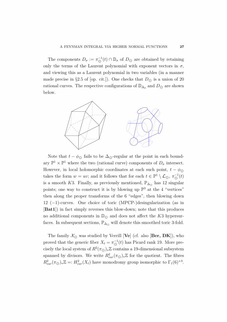
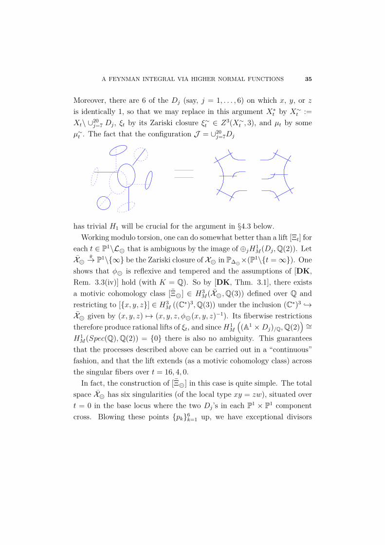
(t) ∩ Dσ of DQ are obtained by retainingonly the terms of the Laurent polynomial with exponent vectors in σ,and viewing this as a Laurent polynomial in two variables (in a mannermade precise in §2.5 of [op. cit.]). One checks that DQ is a union of 20rational curves. The respective configurations of D∆φ

and DQ are shownbelow.

Note that t − φQ fails to be ∆Q-regular at the point in each bound-ary P1 × P1 where the two (rational curve) components of Dσ intersect.However, in local holomorphic coordinates at each such point, t − φQtakes the form w = uv; and it follows that for each t ∈ P1 \ LQ, π

−1Q

(t)is a smooth K3. Finally, as previously mentioned, P∆Q has 12 singularpoints; one way to construct it is by blowing up P3 at the 4 “vertices”then along the proper transforms of the 6 “edges”, then blowing down12 (−1)-curves. One choice of toric (MPCP-)desingularization (as in[Bat1]) in fact simply reverses this blow-down; note that this producesno additional components in DQ and does not affect the K3 hypersur-faces. In subsequent sections, P∆Q will denote this smoothed toric 3-fold.

The family XQ was studied by Verrill [Ve] (cf. also [Ber, DK]), whoproved that the generic fiber Xt = π−1

Q(t) has Picard rank 19. More pre-

cisely the local system of R2(πQ)∗Z contains a 19-dimensional subsystemspanned by divisors. We write R2

var(πQ)∗Z for the quotient. The fibresR2var(πQ)∗Z =: H2

var(Xt) have monodromy group isomorphic to Γ1(6)+3.


The intersection form is H ⊕ 〈6〉 with discriminant 6. In particular, XQis a family of M6 := E8(−1)⊕2 ⊕ H ⊕ 〈−6〉-polarized K3 surfaces, andis thus of Shioda-Inose type (cf. [Mo]). There are countably many t forwhich the Picard rank is 20. For these fibres, the transcendental partH2tr(Xt) is a quotient of H2

var of rank 2. The motive H2tr(Xt) for these

fibres has complex multiplication, i.e. the rational endomorphism ring isan imaginary quadratic field.

We describe a modular construction of such a family, closely relatedto that of [DK, sec. 8.2.2]. Set

α3 := √

3 2√3

−2√

3 −√

3

, β3 := −√3 1√

3−4√

3√

3

, µ6 := 0 −1√

6√6 0

and note that

(3.2.1)

β3µ6 = µ6α3

β−13 α3 =

(5 318 11

)∈

−1 00 −1

Γ1(6).

We have α3(τ) = − τ+ 23

2τ+1 , µ6(τ) = −16τ . These induce involutions on Y1(6)

since

(3.2.2)Γ1(6) C Γ1(6)+3 := 〈Γ1(6), α3〉M M

〈Γ1(6), µ6〉 =: Γ1(6)+6 C Γ1(6)+3+6 := 〈Γ1(6), α3, µ6〉

and α23 =

−1 00 −1

= µ26. (The action on cusps is [i∞] ↔ [1

2 ],

[0] ↔ [13 ] for α3 and [i∞] ↔ [0], [1

2 ] ↔ [13 ] for µ6.) From (3.2.1) one

deduces that these involutions commute; and so µ6 descends to Y1(6)+3 :=〈α3〉\Y1(6)∗α3 and α3 to Y1(6)+6 := 〈µ6〉\Y1(6)∗µ6 , where “∗” means todelete fixed (elliptic) points.

Let ′E1(6)′π1 Y1(6) be the fiber-pullback of π1 by α3. (Note that α3

and µ6 do not lift to involutions of E1(6), but do lift to 3 : 1 resp. 6 : 1


fiberwise isogenies.) Put ′E [2]1 (6) := E1(6) ×

Y1(6)′E1(6), and let

I[2]3 : ′E [2]

1 (6)∼=→ ′E [2]

1 (6)

be the involution given by

(τ ; [z1]τ , [z2]α3(τ)) 7→ (α3(τ); [z2]α3(τ), [z1]τ ).

A first approximation to the three-banana family is then

E [2]1 (6)+3 := I

[2]3

∖′E [2]

1 (6)∗α3π2 Y1(6)+3.

It has fibers of type E[τ ] × E[α3(τ)], hence intersection form H ⊕ 〈6〉 onH2var, and the same local system as R2

var(πQ)∗ZXQ . By Schur’s lemma andthe Theorem of the Fixed Part [Sc], a C-irreducible Z-local system canunderlie at most one polarized Z-variation of Hodge structure, makingthe two variations isomorphic.

However, π2 is not yet a family of K3 surfaces. Quotienting fibers by(−id)2 and resolving singularities yields a family of KummerK3 surfaces,with (incorrect) intersection form (H ⊕ 〈6〉)[2] on H2

var,Z. To correct thismultiplication by 2, we require a fiberwise-birational 2 : 1 cover of theKummer family, which is the Shioda-Inose family [Mo] X1(6)+3 overY1(6)+3. Since this is a family of M6-polarized K3 surfaces with integralH2 isomorphic to πQ, the relevant global Torelli theorem (cf. [Do, Cor.3.2]) yields an isomorphism

X1(6)+3

π

∼=

HQ // XQπQ

Y1(6)+3HQ

∼=// P1 \ LQ.

Explicitly, the Hauptmodul (mapping [i∞] 7→ ∞, [0] 7→ 0, ellipticpoints7→ 4, 16) is given by (2.3.11) and we have the relation

(3.2.3) t = −64t(t − 9)(t − 1) .


This relation between the Hauptmoduls of Feynman integrals with twoand three loops was obtained more than 40 years ago by Geoffrey Joyce,who established a corresponding result for honeycomb and diamond lat-tices in condensed matter physics, exploiting results on integrals of Besselfunctions by Wilfrid Norman Bailey in the 1930s. For further details ofthe striking relationships between Feynman integrals and lattice Greenfunctions, see [BBDG].

3.3. Miscellany. — Two observations about HQ are in order. Thefirst (used below in §5.2) is that we may construct a family X → Y1(6)+3

of smooth surfaces mapping onto X1(6)+3 and E [2]1 (6)+3 (over Y1(6)+3),

with both projections generically 2 : 1 on each fiber. We may thentransfer generalized algebraic cycles from E [2]

1 (6)+3 to XQ by composingthis correspondence withHQ; and the Abel-Jacobi maps are then relatedby the action of this correspondence on cohomology (which is an integralisomorphism on H2

tr after multiplication by 12). To obtain the family X ,

we take (a) the fiber product Ea of E [2]1 (6)+3 and the Kummer family over

E [2]1 (6)+3/〈(−id)×2〉 and (b) the fiber product Eb of the Kummer family

and X1(6)+3 over the quotient of X1(6)+3 by the Nikulin involution (cf.[Mo]). Smoothing these families yields Ea and Eb, whose fiber productover the Kummer family followed by resolution of singularities yields X .

The second observation(4) is that we may use HQ to perform a rationalinvolution on relative cohomology of the family over the automorphismµ : t 7→ 43

tinduced by µ6. First of all, XQ does not itself have a bira-

tional involution over µ, since H2var(Xt,Z) ∼= H2

var(Eτ × Eα3(τ),Z) and

(4)This is not used in the sequel, but illustrates an important difference between thisfamily and the Apéry family of K3 surfaces (cf. [DK]), which does admit such aninvolution.


H2var(X 1

43t,Z) ∼= H2

var(Eµ6(τ) × Eα3(µ6(τ)),Z) are rationally but not inte-grally isomorphic. In particular, we only have a correspondence

E [2]1 (6)+3 //

E [2]1 (6)+3

Y1(6)+3 µ6

∼=// Y1(6)+3

which is a 2 : 1 isogeny in the first factor and 1 : 2 multivalued map inthe second factor, given by(τ ; [z1]τ , [z2]α3(τ)

)7→

µ6(τ);[

(2τ + 1)z2

τ

]µ6(τ)

,

[z1

2(−3τ + 1)

]α3(µ6(τ))

.However, the graph of this correspondence is a family of abelian sur-faces, mapping fiberwise 2 : 1 onto both E [2]

1 (6)+3 and its µ6-pullback,which does have an involution over µ6. This family, or its associatedShioda-Inose K3 family, can then be used as a correspondence (inducingisomorphisms of rational H2

tr) between X1(6)+3 and its µ6-pullback overY1(6)+3.

Finally, for future reference we shall write down a family of holomor-phic 2-forms on the fibers of πQ. For any t ∈ P1 \ LQ, let

(3.3.1) ωt := ResXt

dxx∧ dy

y∧ dz

z

1− t−1φQ

be the standard residue form. Remark that the holomorphic period inthe neighborhood |t| > 16 of t = ∞ may be computed by integrat-ing 1

2πi

dxx∧ dyy∧ dzz

1−t−1φQover the product (S1)×3 of unit circles. By the Cauchy

residue theorem, this is

(3.3.2) (2πi)2 ∑k≥0

akt−k,

where ak, given in (2.3.13), is the constant term in (φQ)k.


4. The three-banana integral as a higher normal function

In this section we shall explain the precise relationship between theintegral IQ and the family XQ ofK3 surfaces defined by the denominatorof the integrand. Properly understanding this, even without the modulardescription (done in §5), leads at once to the inhomogeneous equation(§4.3) and the special values at t = 0 and 1 (§7).

There are a number of general comments. The integral IQ (2.1.6) isa period, i.e. the integral of a rational differential form ω on a varietyP over a chain c whose boundary ∂c is supported on a proper closedsubvariety Σ ⊂ P . This theme goes back to Abel’s theorem on Riemannsurfaces. For Abel, P is a Riemann surface, Σ = p, q ⊂ P is a set oftwo points, ω is a holomorphic 1-form on P and c is a path from p toq. In modern terms, this process associates to the 0-cycle (p) − (q) anextension of Hodge structures

0→ H1(P,Q(1))→ H → Q(0)→ 0.

The second point is that dependence on external momenta means that wehave a family of integrals depending on a parameter t. The correspondingfamily of extensions is called a normal function and first appeared in thework of Poincaré [P, G2].

Finally, it turns out that the three-banana amplitude is associatedto a generalized normal function arising from a family of “higher” alge-braic cycles or motivic cohomology classes [KL, DK]. The passage fromclassical normal functions associated to families of cycles to normal func-tions associated to motivic classes suggests interesting new links betweenmathematics and physics (op.cit.). For one thing, motivic normal func-tions can, in many cases, be associated with multiple-valued holomorphicfunctions which arise as amplitudes. For a discussion of normal functionsin physics, cf. [MW] for instance.


Briefly, the higher Chow groups CHp(X, q) of a variety X over a fieldk are the homology groups of a complex Zp(X, •). By definition Zp(X, q)is the free abelian group on irreducible codimension p subvarieties V →X× (P1 \1)q meeting faces properly, where faces are defined by settingvarious P1-coordinates to be 0 or ∞. Elements of Zp(X, q) are called(higher Chow) precycles. The face maps Zp(X, q) → Zp(X, q − 1) aredefined by restrictions to faces with alternating signs; elements of thekernel are called (higher Chow) cycles.

If f1, . . . , fp are rational functions on X, the locus x, f1(x), . . . , fp(x)will (assuming the zeroes and poles of the fi are in general position)define a precycle in Zp(X, p). The easiest way for its image under theface map to vanish, so that this precycle is a cycle and represents aclass in CHp(X, p), is for the fi to be units (invertible functions) on thecomplement of the the subvariety of X defined by ∏p

j=1(fj(x) − 1) =0. A basic theorem of Suslin and Totaro identifies CHp(Spec k, p) ∼=KMp (k), the p-th Milnor K-group of the field k. These groups are linked

to algebraic K-theory via the γ-filtration

CHp(X, q)⊗Q ∼= grpγKq(X).

Finally, in keeping with modern usage, we will define motivic cohomol-ogy by

HrM(X,Z(s)) := CHs(X, 2s− r)

when X is smooth. Notice that HrM(X,Z(r)) = CHr(X, r) in this case.

More generally, HrM(X,Q(s)) may be constructed from higher Chow pre-

cycles as described in §1.3 of [DK], which leads to a long-exact sequenceused only briefly at the end of §4.1 below.

4.1. K3 of a K3!— Let Xt = π−1Q

(t) (t ∈ P1\LQ) be as in §3.2,X∗t := Xt ∩ (C∗)3 = Xt\DQ, DQ = ∪20

j=1Dj (Dj∼= P1). The Milnor


symbol

x|Xt , y|Xt , z|Xt ∈ KM3 (C(Xt)) ∼= lim−→

U ⊂ XtZar. op.

H3M(U,Z(3))

extends to a (cubical) higher Chow cycle

[ξt] :=[∆(C∗)3 ∩X∗t ×3

]∈ CH3(X∗t , 3) = H3

M(X∗t ,Z(3)),

where := P1\1 and [· · · ] denotes cycle class. To (integrally) lift [ξt]to a class

[Ξt] ∈ H3M(Xt,Z(3))

in the exact sequence(5)

⊕jH1M(Dj,Z(2))→ H3

M(Xt,Z(3))→ H3M(X∗t ,Z(3)) Tame→ ⊕jH2

M(D∗j ,Z(2)),

we must check vanishing of the TameD∗j ([ξt]). Inspection of the edgepolynomials [DK, sec. 2.5] shows that these are all of the form ±u, 1,1,±v, and ±u, 1− (±u) (in toric coordinates u, v on D∗j ∼= (C∗)2),which are trivial.

On the cycle level, the mechanism by which the lift takes place isgiven by the moving lemma for higher Chow groups [Blo2]. This yieldsa quasi-isomorphism

Z3(X∗t , •)'←∗Z3(Xt, •)/ıD∗ Z2(DQ, •)

inducing the above exact sequence, and there exists µt ∈ Z3(X∗t , 4) suchthat(6)

ξt + ∂µt = ∗Ξt.

(5)The ambiguities of this lift by the images of the H1M (Dj ,Z(2)) may for our purposes

be ignored, as they have no bearing upon the transcendental part of its Abel-Jacobiimage.(6)Note: in this paper “∂” is used both to denote the boundary of a C∞ cochain andthe differential in the higher Chow complex.


Moreover, there are 6 of the Dj (say, j = 1, . . . , 6) on which x, y, or zis identically 1, so that we may replace in this argument X∗t by X∼t :=Xt\ ∪20

j=7 Dj, ξt by its Zariski closure ξ∼t ∈ Z3(X∼t , 3), and µt by someµ∼t . The fact that the configuration J = ∪20

j=7Dj

has trivial H1 will be crucial for the argument in §4.3 below.Working modulo torsion, one can do somewhat better than a lift [Ξt] for

each t ∈ P1\LQ that is ambiguous by the image of ⊕jH1M(Dj,Q(2)). Let

XQπ→ P1\∞ be the Zariski closure of XQ in P∆Q×(P1\t =∞). One

shows that φQ is reflexive and tempered and the assumptions of [DK,Rem. 3.3(iv)] hold (with K = Q). So by [DK, Thm. 3.1], there existsa motivic cohomology class [ΞQ] ∈ H3

M(XQ,Q(3)) defined over Q andrestricting to [x, y, z] ∈ H3

M ((C∗)3,Q(3)) under the inclusion (C∗)3 →XQ given by (x, y, z) 7→ (x, y, z, φQ(x, y, z)−1). Its fiberwise restrictionstherefore produce rational lifts of ξt, and sinceH1

M

((A1 ×Dj)/Q,Q(2)

) ∼=H1M(Spec(Q),Q(2)) = 0 there is also no ambiguity. This guarantees

that the processes described above can be carried out in a “continuous”fashion, and that the lift extends (as a motivic cohomology class) acrossthe singular fibers over t = 16, 4, 0.

In fact, the construction of [ΞQ] in this case is quite simple. The totalspace XQ has six singularities (of the local type xy = zw), situated overt = 0 in the base locus where the two Dj’s in each P1 × P1 componentcross. Blowing these points pk6

k=1 up, we have exceptional divisors


Ek ∼= P1 × P1 (k = 1, . . . , 6) in ˜XQ, and the long exact sequence⊕k

H2M(Ek,Q(3))→ H3

M(XQ,Q(3))→

H3M( ˜XQ,Q(3))⊕

⊕k

H3M(pk,Q(3)) α→

⊕k

H3M(Ek,Q(3)).

One easily lifts [x, y, z] to [ΞQ] ∈ H3M( ˜XQ,Q(3)) (since the Tame sym-

bols vanish), whereupon α([ΞQ], 0) vanishes since x, y, or z was 1 at eachpk.

In the sequel, the restriction of [ΞQ] to H3M(XQ,Q(3)) will be denoted

by [ΞQ]; we call this the three-banana cycle.

4.2. Review of Abel-Jacobi. — We shall need a few generalities onregulator currents for the arguments below. The presentation will besketchy, as a more thorough exposition may be found in [DK, sec. 1].

Let X be a smooth projective variety with complexes of currentsD•(X) and (2πi)pA-valued C∞-cochains C•top(X;A(p)) (A ⊂ R a sub-ring). Given a cochain γ, we write δγ for the current of integration overit, and use this to define the Deligne complex

C•D(X,A(p)) :=(C•+1top (X;A(p))⊕ F pD•+1(X)⊕D•(X)

)[−1]

with differential

(4.2.1) D(T,Ω, R) := (∂T,−d[Ω], d[R]− Ω + δT ).

Its (2p− n)th cohomology sits in a short-exact sequence

0→ Jp,n(X)A → H2p−nD (X,A(p))→ Hgp,n(X)A → 0,

where Hgp,n(X)A := HomA-MHS(A(0), H2p−n(X,A(p)))Jp,n(X)A := Ext1A-MHS(A(0), H2p−n−1(X,A(p)))

.

Let Zp(X, •) be the codimension-p higher Chow cycle complex withnth homology CHp(X,n) = H2p−n

M (X,Z(p)), and boundary map ∂; in


particular, Zp(X,n) is a subgroup of the cycle group Zp(X×n). Denoteby Zp

R(X, •) ⊂ Zp(X, •)Q the quasi-isomorphic subcomplex(7) describedin [KL, sec. 8.2]. By [KLM, sec. 7], the cycle class map

cp,nD : CHp(X,n)Q = H2p−nM (X,Q(p))→ H2p−n

D (X,Q(p))

defined in [Blo1] is computed by a map of complexes

ZpR(X, •)→ C2p−•

D (X,Q(p)).

Taking • = n, it is defined on irreducible components by(8)

(4.2.2) ξ 7−→ (2πi)p−n ((2πi)nTξ,Ωξ, Rξ) ,

where (writing πX , π for the projections from a desingularization ξ toX, n) Rξ [resp. Ωξ, Tξ] is defined by applying (πX)∗(π)∗ to(9)

Rn :=n∑j=1

((−1)n2πi)j−1 log(zj)dzj+1

zj+1∧ · · · ∧ dzn

znδTz1∩···∩Tzj−1

resp. Ωn :=n∧j=1

dzjzj, Tn :=

n⋂j=1

Tzj :=n⋂j=1

z−1j (R<0)

.Properties of Tn,Ωn, Rn imply that

(4.2.3) d[Rξ] = Ωξ − (2πi)nδTξ + 2πiR∂ξ,

so that (by (4.2.1)) (4.2.2) gives a map of complexes.Suppose ∂ξ = 0 (so that [ξ] ∈ H2p−n

M (X,Q(p))) and n ≥ 1. Since [Tξ]and [Ωξ] define the map to Hgp,n(X)Q(which is zero for n ≥ 1), thereexistK ∈ F pD2p−n−1(X) and Γ ∈ C2p−n−1

top (X;Q(p)) such that Ωξ = d[K]

(7)These are still precycles with Q-coefficients; the “R” refers to intersection conditionswith real-analytic chains.(8)This differs from the formula in [KLM] by a (2πi)− dim(X) twist arising there fromPoincare duality, since we interpret currents here as computing cohomology, not ho-mology. (This choice is more convenient for computation.)(9)Here log(z) is regarded as a 0-current on P1 with branch cut along R<0, so thatd[log(z)] = dz

z − 2πiδTz. Operations involving pullback are not in general defined on

currents, but a convergence argument (when ξ is in the subcomplex) shows that Rξand Ωξ are in fact currents on X.


and Tξ = ∂Γ, whereupon

Rξ := Rξ −K + (2πi)nδΓ

defines a closed current with class [Rξ] ∈ H2p−n−1(X,C) projecting to

(cp,nD (ξ) =)AJp,nX (ξ) ∈ Jp,n(X)Q ∼=H2p−n−1(X,C)

F pH2p−n−1(X,C) +H2p−n−1(X,Q(p)) .

If X is a smooth algebraic K3 surface and p = n = 3, then

(4.2.4) AJ3,3X : H3

M(X,Z(3))→ H2(X,C/Z(3)) = J3,3(X)

is computed by

(4.2.5) Rξ := Rξ + (2πi)3δΓ,

since Ωξ ∈ F 3D3(X) = 0. Let U ⊂ X be a Zariski open set. Anyprecycle ξ ∈ Z3

R(U, 3) is a sum of components supported over divisorsand components with generic support. The simplest examples of thelatter are elements of the form

f1, f2, f3U := (x, f1(x), f2(x), f3(x)) |x ∈ U\ ∪ |(fi)|,

where fi ∈ C(X)∗ and the bar denotes Zariski closure in U × 3. Onecan show that

Rf1,f2,f3 = log(f1)df2

f2∧ df3

f3+ 2πi log(f2)df3

f3δTf1 + (2πi)2 log(f3)δTf1∩Tf2

extends to a 2-current on X (even if the closure of f1, f2, f3U over Xis not a precycle).

This has the following application to the general situation of §4.1,where ξ = f1, f2, f3U = ∗Ξ − ∂µ for Ξ ∈ ker(∂) ⊂ Z3

R(X, 3) andµ ∈ Z3

R(U, 4), under the assumption that ∩jf−1j (R<0) ∩ U = ∅. Working

modulo currents and chains supported on D := X\U , formally applying(4.2.2) (and noting that Rµ extends to X) gives

(4.2.6)((2πi)3Tξ, 0, Rξ

)+D

((2πi)3Tµ, 0,

12πiRµ

)≡((2πi)3TΞ, 0, RΞ

),


while our assumption gives Tξ ≡ 0. For the chains, this yields TΞ =−∂Tµ + SD, where SD is a (closed) 1-chain supported on D; since TΞ isexact, so is SD (on X), and we write SD = ∂γ. For the currents, (4.2.6)gives

RΞ = Rξ + 12πid[Rµ] + (2πi)3δTµ +KD

for some 2-current KD supported on D, so that (taking Γ = −Tµ + γ in(4.2.5))

RΞ = Rξ + 12πid[Rµ] + (2πi)3δγ +KD

gives a lift of AJ3,3X (Ξ).

The key point is now that if H1(D) = 0, then we may take γ to besupported on D, and up to exact currents on X and arbitrary currentssupported on D,

(4.2.7) RΞ ≡ Rf1,f2,f3.

This is precisely what occurs in §4.1 with X = Xt, Ξ = Ξt = ΞQ|Xt ,U = X∼t , D = J , and f1, f2, f3 = x|X∼t , y|X∼t , z|X∼t ; the assumptionTx,y,z ≡ 0 holds for

t /∈ φQ(R×3<0) = [16,∞] .

Writing

AJ3,3Xt := πvar AJ3,3

Xt : H3M(Xt,Q(3))→ H2

var(Xt,C/Q(3)),

(4.2.7) provides a well-defined lift (for t /∈ [16,∞] ∪ 0, 4)

Rt := πvar[RΞt ] ∈ H2var(Xt,C)

of Rt := AJ3,3Xt (Ξt). As the extension of R2

var(πQ)∗Q across t = 0 hasonly rank 1, and Rt must extend through t = 0, we conclude part (i) ofthe


Proposition 4.2.1. — (i) Rt yields a holomorphic section of the sheafO⊗R2

var(πQ)∗C over P1\[16,∞]∪ 0, 4, and is the unique such sectionlifting Rt with no monodromy about t = 0 and t = 4.(ii) Writing δt := t d

dtand ∇ for the Gauss-Manin connection, we have

∇δtRt = −[ωt],

with ωt := ResXt

(dxx∧ dyy∧ dzz

1−t−1φQ

).

Proof. — (ii) follows at once from [DK, Cor. 4.1] (note tDK = t−1).

4.3. Reinterpreting the Feynman integral. — The term “highernormal function” has been used in several different ways in the theory ofalgebraic cycles – for instance, to describe the section of ∪tJ3,3(Xt) (i.e.the family of extension classes (4.2.4)) associated to a family of highercycles like Ξt. Here we shall pair this section with a specific familyof holomorphic forms to get an actual function (Definition 4.3.1). Wepreface this with a brief discussion of the pairings used here and in latersections.

Let X be a smooth projective surface, [X] ∈ H4(X,Q) its fundamentalclass, and ˆ

[X]: H4(X,Q)→ Q(0)

the map (of Hodge type (−2,−2)) induced by pairing with [X]. We candefine a Poincaré pairing in one of two ways:

〈 , 〉 : H2(X,Q)×H2(X,Q)→ H4(X,Q)´[X]→ Q(0) ;

〈 , 〉′ : H2(X,Q)×H2(X,Q)→ H4(X,Q) = Q(−2).

While the second has type (0, 0), we prefer to work with the first bracket.We now turn to the main content of this subsection.

Definition 4.3.1. — The (truncated) higher normal function associ-ated to ΞQ is

VQ(t) := 〈Rt, [ωt]〉 ∈ O(UQ),


where ωt := −1(2πi)2t

ωt ∈ Ω2(Xt) and UQ ⊂ P1 \ LQ = P1 \ 0, 4, 16,∞ isthe complement of the real segment 16 < t <∞.

Note that VQ extends holomorphically across t = 4 and 0, since itpairs finite (in fact nonzero) homology resp. cohomology classes ([ω′t]resp. Rt) on those singular fibers.

Theorem 4.3.2. — IQ(t) = VQ(t) on UQ.

Proof. — Begin by noting that

ωt = −1(2πi)2ResXt

dxx∧ dy

y∧ dz

z

t− φQ(x, y, z)

=: ResXt(Ωt

)so that (regarding Ωt ∈ F 3D3(P∆Q) as a 3-current)

d[Ωt

]= 2πiıXt∗ ωt.

Furthermore, R∗3 := Rx,y,z extends to a 2-current on P∆Q , and writingΩ∗3 := dx

x∧ dy

y∧ dz

z, T ∗3 := Tx ∩ Ty ∩ Tz, we have on P∆Q

(4.3.1) d[R∗3] = Ω∗3 − (2πi)3δT ∗3 +KD,

where KD (∈ F 1D3(P∆Q)) is supported on DQ.Now(10) IQ(t) =

=ˆR×3<0

dxx∧ dy

y∧ dz

z

t− φQ(x, y, z) = −(2πi)2ˆT ∗3

Ωt

= −(2πi)2ˆP∆Q

δT ∗3 ∧ Ωt.

By (4.3.1), this

= 12πi

ˆP∆Q

(d[R∗3]− Ω∗3 −KD) ∧ Ωt.

(10)The apparent sign change in the denominator (compare (2.2.1)) arises from theorientation of T ∗3 and the change of variables.


Noting that KD ∧ Ωt and Ω∗3 ∧ Ωt are zero by type, it becomes

= 12πi

ˆP∆Q

d[R∗3] ∧ Ωt

= 12πi

ˆP∆Q

R∗3 ∧ d[Ωt]

=ˆP∆Q

R∗3 ∧ ıXt∗ ωt

(4.3.2) =ˆXt

Rx|X∼

t,y|X∼

t,z|X∼

t

∧ ωt.Finally, the argument of (4.2.7)ff allows us to rewrite this as

=ˆXt

RΞt ∧ ωt = VQ(t).

Without the last step, (4.3.2) would not pair two closed currents andwould have no cohomological meaning. So the seemingly bizarre criterionthat H1(J ) = 0, in the end, is absolutely essential.

To give an idea of the power of Theorem 4.3.2, we conclude this sectionwith one of its basic consequences: namely, an alternate proof of Theorem2.2.1. The characterization of IQ as a higher normal function can alsobe used to compute some special values, cf. §7.

For deriving the Picard-Fuchs equation, we shall modestly abuse no-tation and regard the family of forms as a section

ωt ∈ Γ(P1\LQ,O ⊗R

2var(πQ)∗C

).

Let ∇PF be the operator on cohomology obtained from DPF := L3t =∑3

k=0 fk(t) dk

dtkby replacing d

dtby ∇t := ∇ d

dt, so that by [Ve, Prop. 8]

∇PF ωt = 0. Note that f3(t) = t2(t− 4)(t− 16) and f2(t) = 6t(t2− 15t+


32) = 32f′3(t). Introduce the Yukawa coupling

Y (t) := 〈ωt,∇2t ωt〉,

which may be computed as follows. Observe that by type 0 = 〈ωt,∇tωt〉implies

0 = d2

dt2〈ωt,∇tωt〉 = 〈ωt,∇3

t ωt〉+ 3〈∇tωt,∇2t ωt〉,

so thatd

dtY (t) = 〈ωt,∇3

t ωt〉+ 〈∇tωt,∇2t ωt〉 = 2

3〈ωt,∇3t ωt〉

implies

f3(t)Y ′(t) = 23〈ωt,−f2(t)∇2

t ωt − f1(t)∇tωt − f0(t)ωt〉

= −f ′3(t)Y (t)

that impliesY (t) = κ

f3(t) ∈ C(t).

We will see below in §5.2 that κ = −24(2πi)2 . Assuming this, we conclude

Corollary 4.3.3. — DPF

(IQ(t)

)= −24.

Proof. — By Prop. 4.2.1(ii),

∇tRt = (2πi)2ωt.

Now IQ(t) = VQ(t) = 〈Rt, ωt〉, andd

dt〈Rt, ωt〉 = (2πi)2〈ωt, ωt〉+ 〈Rt,∇tωt〉 = 〈Rt,∇tωt〉

d2

dt2〈Rt, ωt〉 = (2πi)2〈ωt,∇tωt〉+ 〈Rt,∇2

t ωt〉 = 〈Rt,∇2tωt〉

by type (and Griffiths transversality [G]). Together with

d3

dt3〈Rt, ωt〉 = (2πi)2Y (t) + 〈Rt,∇3

t ωt〉,


these give

DPF 〈Rt, ωt〉 = 〈Rt,∇PF ωt〉+ (2πi)2f3(t)Y (t)

= (2πi)2f3(t)Y (t) = −24.

Remark 4.3.4. — For later reference we note that Y (t) := 〈ωt,∇2δtωt〉 =

(2πi)4t4Y (t) =⇒ Y (∞) = (2πi)4κ.

5. A second computation of the three-banana integral: theEisenstein symbol

As an application of the results in sections 3 and 4, we will use HQ topull back the toric three-banana cycle ΞQ ∈ H3

M(XQ,Q(3)) to X1(6)+3.We then apply a correspondence to produce a higher Chow cycle on aKuga variety E [2](6) (defined below), and recognize this as an Eisensteinsymbol in the sense of Beilinson [Beil, DS, DK]. This will allow us towrite the pullback V HQ of the higher normal function (i.e. Feynmanintegral) as an elliptic trilogarithm, giving another proof of Theorem2.3.2.

5.1. Higher normal functions of Eisenstein symbols. — For sim-plicity of exposition we shall restrict to the setting of Kuga 3-folds. Webegin with an explanation of Beilinson’s construction of higher cycles("Eisenstein symbols") on these 3-folds and their relationship to Eisen-stein series of weight 4. Each such cycle gives rise to a higher normalfunction over a modular curve (defined in (5.1.3)), which turns out tobe an Eichler integral of the corresponding Eisenstein series. The mainresult of this subsection, Proposition 5.1.1, computes the q-expansion(5.1.5) of this normal function. In many cases it may be rewritten interms of trilogarithms (cf. theorems 2.3.2 and 5.3.1). Everything in this


subsection is general. In §§5.2-5.3 we shall apply this general compu-tation to our special case, by pulling back the three-banana cycle fromXQ to the Kuga 3-fold and interpreting the result (up to Abel-Jacobiequivalence) as one of Beilinson’s cycles.

To describe these cycles, consider the elliptic modular surface E(N) :=(Z2oΓ(N))\(C×H) over Y (N) = Γ(N)\H, where Γ(N) = kerSL2(Z)→SL2(Z/NZ) and N > 3. Its fibers are elliptic curves with 1-form dz andstandard Betti 1-cycles α = [0, 1], β = [0, τ ]. By duality we may regardα, β as defining H1 classes, and write [dz] = [β]− τ [α].

Let E [2](N) π[2](N)−→ Y (N) be the self-fiber product of E(N). Thereexists a semistable compactification E [2](N) → Y (N) due to Shokurov[Sh], with singular fibers D[2](N) = E [2](N)\E [2](N). Choose for each

cusp σ =[rs

]∈ κ(N) := Y (N)\Y (N) an element Mσ :=

p q

−s r

∈SL2(Z). Define modular forms of weight n for Γ(N) by

Mk(N) :=

F ∈ O(H)

∣∣∣∣∣∣(i) F (τ) = F (γ(τ))

(cτ+d)k =: F |kγ (∀γ ∈ Γ(N))(ii) rσ(F ) := lim

τ→i∞F |kMσ−1 <∞ (∀σ ∈ κ(N))

.There is an isomorphism ([Sh], or [DK, Prop. 7.1])

Ψ : M4(N)∼=→ Ω3(E [2](N))〈logD[2](N)〉

F (τ) 7→ (2πi)3F (τ)dz1 ∧ dz2 ∧ dτ.

Let ΦK2 (N) denote the vector space ofK-valued functions on (Z/NZ)2,

with subspaces ΦK2 (N) := kerevaluation at (0, 0) and

ΦK2 (N) := keraugmentation =

f : (Z/NZ)2 → K |∑

0≤m,n≤N−1f(m,n) = 0


Assuming K ⊃ Q(ζN) (ζN := e2πiN ), these are exchanged by the finite

Fourier transform

ϕ(m,n) 7→ ϕ(µ, η) :=∑

(m,n)∈(Z/NZ)2

ϕ(m,n)ζµn−ηmN .

This allows us to define the Q-Eisenstein series EQ4 (N) by the image of

the map

E : ΦQ2 → M4(N)

ϕ 7→ Eϕ(τ) := − 3(2πi)4

∑(m,n)∈Z2\(0,0)

ϕ(m,n)(mτ + n)4 .

The horospherical maps

Hσ : ΦQ2 (N) → Qϕ 7→ Hσ(ϕ) := 1

8∑N−1a=0 B4

(aN

)· ((πσ)∗ϕ)(a)

record the “values” limτ→i∞Eϕ(τ)|4M−1σ

(= Hσ(ϕ)) of the Eisenstein seriesEϕ at the cusps. Here πσ : (Z/NZ)2 Z/NZ sends (m,n) = a(p, q) +b(−s, r) 7→ a, while (πσ)∗ sums along fibers of πσ, and B4(x) = x4−2x3 +x2 − 1

30 is the fourth Bernoulli polynomial. Alternatively, one has

Hσ(ϕ) = − 6(2πi)4L(ι∗σϕ, 4)

where ισ : Z/NZ → (Z/NZ)2 sends a 7→ a(−s, r) and

L(φ, n) :=∑k≥1

φ(k)kn

.

To construct the cycles, let U ⊂ E(N) [resp. U [2] ⊂ E [2](N)] be thecomplement of the N2 [resp. N4] N -torsion sections over Y (N). Fixϕ ∈ ΦQ

2 (N), and (thinking of it as a Q-divisor supported on E(N)\U)let mα ∈ Q and fα1, fα2, fα3 ∈ O∗(U) satisfy ∑

αmα(fα1) ∗ (fα2) ∗(fα3) = ϕ (Pontryagin product). (Here (fαi) is the divisor of fαi, thedivisor being viewed as a function on (Z/NZ)2, and the Pontryaginproduct of two functions on a finite abelian group is defined by (f ∗


g)(a) = ∑b+c=a f(b)g(c). The group(11) G := D4 n (Z/NZ)4 acts on

H3M(U [2],Q(3)), and the G-symmetrization of∑

α

mαfα1(−z1), fα2(z1 − z2), fα3(z2)

extends to a cycle in H3M(E [2](N),Q(3)) (cf. [DK, sec. 7.3.4]). By abuse

of notation we shall call it Zϕ, since its fiberwise AJ3,3-classes

(5.1.1) Rϕ(y) ∈ H2var

(π[2](N)−1(y),C/Q(3)

), y ∈ Y (N),

depend only on ϕ – indeed, only on the Hσ(ϕ)|σ ∈ κ(N) – and notthe choice of fαi [DK, Cor 9.1].(12)

The connection between the cycle Zϕ and the Eisenstein series Eϕcomes about as follows. First, by using the moving lemma [Blo2] andlog complexes of currents, it is possible to extend the (T,Ω, R) calcu-lus of §4.2 to the quasi-projective setting ([KLM, §5.9],[KL, §3.1]). Inparticular, the fundamental class of Zϕ (i.e. the image of c3,3

D (Zϕ) inHg3,3(E [2](N))Q) is computed by the holomorphic (3, 0)-form ΩZϕ . Ac-cording to a result of Beilinson (in the form of [DK, Thm. 8.1]), wehave

(5.1.2) ΩZϕ = Ψ(Eϕ) = (2πi)3Eϕ(τ)dz1 ∧ dz2 ⊗ dτ.

It follows that Rϕ(y) is given (up to an important “constant of integra-tion”) by the Gauss-Manin integral of (5.1.2); that is, (5.1.2) is ∇Rϕ.

Define the associated higher normal function by(13)

(5.1.3) Vϕ(τ) := 〈Rϕ([τ ]), [dz1 ∧ dz2]〉,

(11)D4 denotes the dihedral group of order 8.(12)The reader is warned of the typo “surjective” for “injective” in the statement of[loc. cit., Lemma 9.1(ii)].(13)Note: a priori this just uses the Poincaré pairing H2(E×2

τ ,C)⊗2 → C on eachfiber. However, it is better to think of [dz1∧dz2] as a class in H2(E×2

τ ,C) by Poincaréduality and (5.1.3) as pairing H2 ×H2 → C, since this approach will extend acrossthe singular fibers of E [2](N) over cusps σ for which Hσ(ϕ) = 0.


where for now Rϕ is an indeterminate lift of Rϕ to O ⊗ R2varπ

[2](N)∗C.Arguing as in the proof of Corollary 4.3.3 above, and noting ∇3

τ [dz1 ∧dz2] = 0,

d3

dτ 3Vϕ(τ) = d2

dτ 2 〈Rϕ,∇τ [dz1 ∧ dz2]〉

= d

dτ

⟨Rϕ,∇2

τ [dz1 ∧ dz2]⟩

=⟨(2πi)3Eϕ(τ)[dz1 ∧ dz2], 2[α1 × α2]

⟩(5.1.4) = −2(2πi)3Eϕ(τ).

That is, Vϕ is an Eichler integral of Eϕ. This leads to the following result,which is closely related to [DK, Prop. 9.2].

Proposition 5.1.1. — Assume for simplicity that ϕ(m,n) = ϕ(−m,−n).Then up to a Q(3)-period (2πi)3Q0 + (2πi)2Q1 log q + (2πi)Q2(log q)2

(Qi ∈ Q),

(5.1.5) Vϕ(q) ≡ 2(2πi)4L (ι∗i∞ϕ, 4) (log q)3 + 1

NL ((πi∞)∗ϕ, 3)

+ 2N

∑M≥1 q

MN∑d|M

1d3∑a∈Z/NZ ζ

aMd

N ϕ(d, a).

(Note that 1(2πi)4L(ι∗i∞ϕ, 4) ∈ Q.)

Proof. — By a classical result (cf. [Gu]), we have

(5.1.6) Eϕ(τ) = H[i∞](ϕ)− 1N4

∑M≥1

qMN

∑r|M

r3 ∑a∈Z/NZ

ζarN ϕ(M

r, a).

In accordance with (5.1.4), we must take three indefinite integrals of−2(2πi)3Eϕ(τ) with respect to dτ = 1

2πid log q, i.e. of −2Eϕ(τ) withrespect to d log q. Applying this to the second term of (5.1.6) gives

(5.1.7) 2N

∑M≥1

qMN

M3

∑r|M

r3 ∑a∈Z/NZ

ζarN ϕ(M

r, a),

and replacing r by d = Mr

recovers the sum in (5.1.5). Doing the sameto H[i∞](ϕ) would give −1

3H[i∞](ϕ)(log q)3 plus an arbitrary quadraticpolynomial in log q. The more precise stated result follows at once from


[DK, (9.29)],(14) which is based on the delicate fiberwise AJ3,3 computa-tion for Zϕ carried out in §9.2 of [op. cit.].

The connection of this formula to trilogarithms arises as follows. Define

(5.1.8) Li3(x) :=∑k≥1

Li3(xk) =∑k≥1

∑δ≥1

xkδ

δ3 =∑m≥1

xm∑δ|m

1δ3 ,

and suppose that we can write

ϕ =∑α|Nβ|N

µαβψα,β

where

(5.1.9) ψα,β(m,n) :=

1, if α|m and β|n0, otherwise

.

In the ∑M≥1 term2N

∑α,β

µαβ∑M≥1

qMN

∑d|M

1d3

∑a∈Z/NZ

ζaMd

N ψα,β (d, a)

of (5.1.5), the sum ∑a∈Z/NZ ζ

aMd

N ψα,β(d, a) is zero unless α|d and Nβ|Md

(implies αNβ|M), in which case it is N

β. So after putting M = αN

βm and

d = αδ, the last displayed expression becomes

= 2N

N

β

∑α,β

µαβ∑m≥1

(qαβ

)m∑δ|m

1δ3α3 ,

which (upon putting k = mδ)

(5.1.10) = 2∑α,β

µαββα3 Li3

(qαβ

).

(14)Note that while this formula is derived in [op. cit.] for ϕ of the form 1N π∗i∞ϕ

′, anyϕ is of this form modulo ker(H[i∞]) ⊂ ΦQ

2 (N).


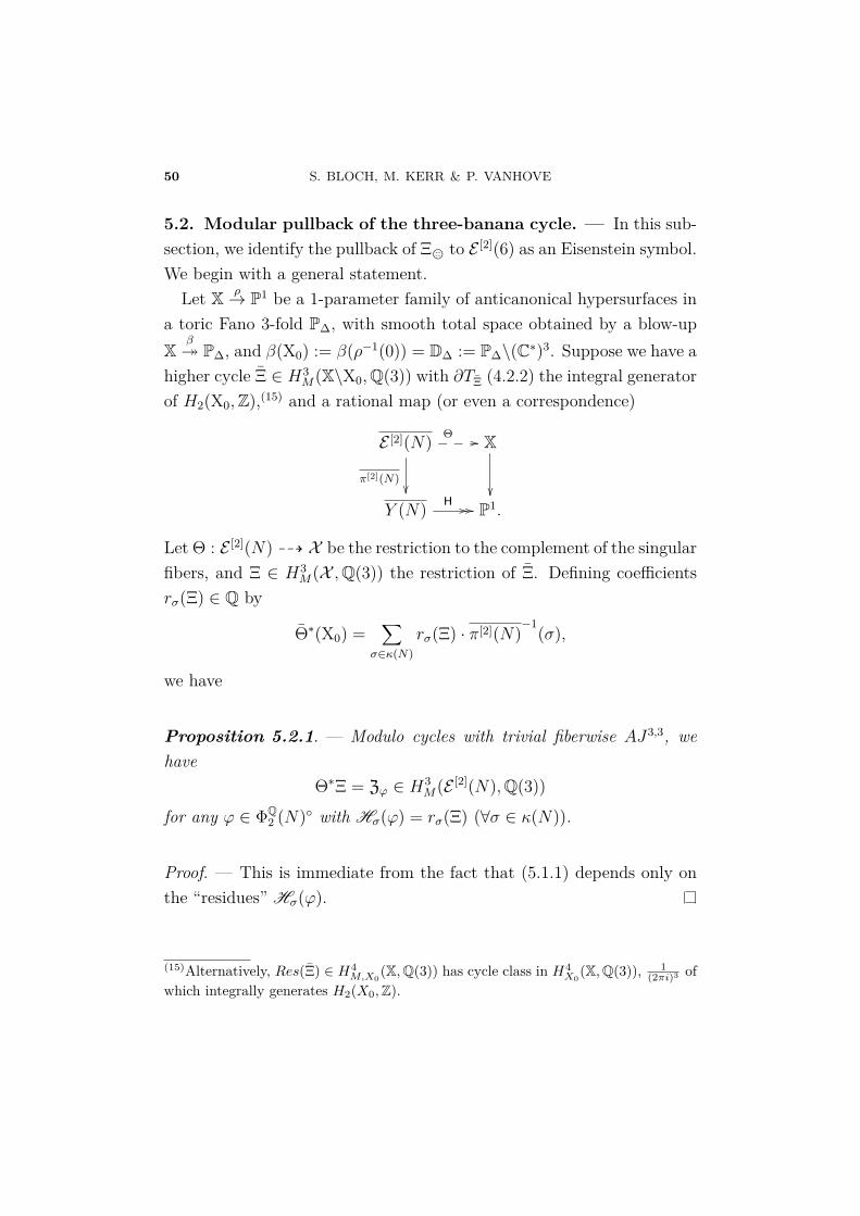
5.2. Modular pullback of the three-banana cycle. — In this sub-section, we identify the pullback of ΞQ to E [2](6) as an Eisenstein symbol.We begin with a general statement.

Let X ρ→ P1 be a 1-parameter family of anticanonical hypersurfaces ina toric Fano 3-fold P∆, with smooth total space obtained by a blow-upX

β P∆, and β(X0) := β(ρ−1(0)) = D∆ := P∆\(C∗)3. Suppose we have a

higher cycle Ξ ∈ H3M(X\X0,Q(3)) with ∂TΞ (4.2.2) the integral generator

of H2(X0,Z),(15) and a rational map (or even a correspondence)

E [2](N) Θ //

π[2](N)

X

Y (N) H // // P1.

Let Θ : E [2](N) 99K X be the restriction to the complement of the singularfibers, and Ξ ∈ H3

M(X ,Q(3)) the restriction of Ξ. Defining coefficientsrσ(Ξ) ∈ Q by

Θ∗(X0) =∑

σ∈κ(N)rσ(Ξ) · π[2](N)−1(σ),

we have

Proposition 5.2.1. — Modulo cycles with trivial fiberwise AJ3,3, wehave

Θ∗Ξ = Zϕ ∈ H3M(E [2](N),Q(3))

for any ϕ ∈ ΦQ2 (N) with Hσ(ϕ) = rσ(Ξ) (∀σ ∈ κ(N)).

Proof. — This is immediate from the fact that (5.1.1) depends only onthe “residues” Hσ(ϕ).

(15)Alternatively, Res(Ξ) ∈ H4M,X0

(X,Q(3)) has cycle class in H4X0

(X,Q(3)), 1(2πi)3 of

which integrally generates H2(X0,Z).


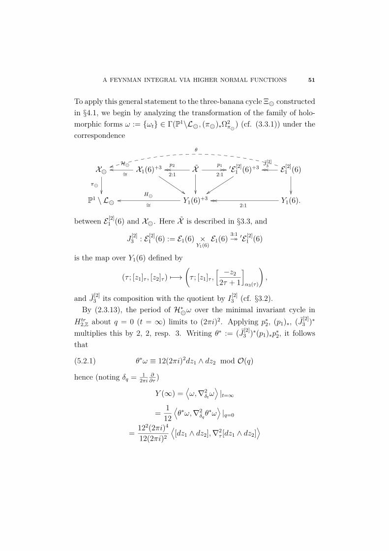
To apply this general statement to the three-banana cycle ΞQ constructedin §4.1, we begin by analyzing the transformation of the family of holo-morphic forms ω := ωt ∈ Γ(P1\LQ, (πQ)∗Ω2

πQ) (cf. (3.3.1)) under the

correspondence

XQπQ

X1(6)+3∼=

HQoo

$$

X

p1

2:1// //

p2

2:1oooo ′E [2]

1 (6)+3

yy

E [2]1 (6)

J[2]3oooo

θ

tt

P1 \ LQ Y1(6)+3∼=

HQoo Y1(6).2:1

oooo

between E [2]1 (6) and XQ. Here X is described in §3.3, and

J[2]3 : E [2]

1 (6) := E1(6) ×Y1(6)E1(6) 3:1

′E [2]1 (6)

is the map over Y1(6) defined by

(τ ; [z1]τ , [z2]τ ) 7−→(τ ; [z1]τ ,

[ −z2

2τ + 1

]α3(τ)

),

and J [2]3 its composition with the quotient by I [2]

3 (cf. §3.2).By (2.3.13), the period of H∗

Qω over the minimal invariant cycle in

H tr2,Z about q = 0 (t = ∞) limits to (2πi)2. Applying p∗2, (p1)∗, (J [2]

3 )∗

multiplies this by 2, 2, resp. 3. Writing θ∗ := (J [2]3 )∗(p1)∗p∗2, it follows

that

(5.2.1) θ∗ω ≡ 12(2πi)2dz1 ∧ dz2 mod O(q)

hence (noting δq = 12πi

∂∂τ)

Y (∞) =⟨ω,∇2

δtω⟩|t=∞

= 112⟨θ∗ω,∇2

δqθ∗ω⟩|q=0

= 122(2πi)4

12(2πi)2

⟨[dz1 ∧ dz2],∇2

τ [dz1 ∧ dz2]⟩


= −24(2πi)2,

where Y (t) was defined in Remark 4.3.4. In fact, by that remark we nowhave κ = −24

(2πi)2 as claimed in the proof of Corollary 4.3.3.

Turning to the computation of the rσ(ΞQ), we take Θ to be thecomposition of θ with the base change over Y (6) Y1(6). We examinethe pullback by Θ of the (3, 0) form ΩΞQ which computes the fundamentalclass of the cycle. By (4.2.3) and Proposition 4.2.1(ii), ΩΞQ = −ω ∧ dt

t∈

Ω3(XQ), and (5.2.1) now gives

ΩΘ∗ΞQ = −Θ∗ΩΞQ = Θ∗ω ∧ dlogHQ(τ)

≡ 12(2πi)3dz1 ∧ dz2 ∧ dτ mod O(q),

which implies at once that r[i∞](ΞQ) = 12. (Note the consistency with(5.1.2) and (5.1.6).) Now the (partial) pullback of ΞQ to ′E [2]

1 (6) is in-variant under I [2]

3 ; a calculation as in [DK, sec. 8.2.2] shows that con-sequently r[− 1

2 ](ΞQ) = r[α3(i∞)](ΞQ) = − r[i∞](ΞQ)32 = −4

3 . In fact, writingΩΘ∗ΞQ = (2πi)3EQ(τ)dz1 ∧ dz2 ∧ dτ , we have EQ(τ) ∈ M4(Γ1(6)+3);and rσ(ΞQ) : κ(6) → Q is the pullback of the function on κ1(6) =

[i∞], [0], [12 ], [1

3 ]taking the respective values 12, 0,−4

3 , 0. (Under κ(6)κ1(6), the preimage of [i∞] resp. [1

2 ] is [i∞] resp.

[12 ], [3

2 ], [−12 ].) Us-

ing the formula for Hσ, one then finds that the function ϕQ on (Z/NZ)2

with Fourier transform

(5.2.2) ϕQ(m,n) :=

−2635/5, (m,n) ≡ (0,±1) mod 62633/5, (m,n) ≡ (±2,±1 or 3) mod 6

0, otherwise

satisfies Hσ(ϕQ) = rσ(ΞQ).Finally we determine the pullbacks of ω and ω. In [Ve], it is shown that

$1(τ) = (η(2τ)η(6τ))4 (η(τ)η(3τ))−2 is the HQ-pullback of a solution toDPF ; so Θ∗(ω) = C · $1(τ)dz1 ∧ dz2 for some constant C. But thenΘ∗(ω) = −(2πi)2C$1(τ)HQ(τ)dz1 ∧ dz2 and by (5.2.1) C = 12.


Remark 5.2.2. — One further immediate consequence is thatEQ(τ) =12$1(τ)

2πidH−1Q

(τ)dτ

= 12+24q−168q2+· · · ; but the equality EQ(τ) = EϕQ(τ)is more useful for us as it allows us to apply Proposition 5.1.1 and getthe “constant of integration” right.

5.3. The main result. — Recall that VQ(t) = 〈Rt, [ωt]〉. Puttingeverything together, we arrive at the

Theorem 5.3.1. — Up to a Q(3)-period (2πi)3Q0+(2πi)2Q1τ+(2πi)Q2τ2

(Qi ∈ Q), we have VQ(HQ(τ))$1(τ) =

−4(log q)3 + 16ζ(3)− 16

2Li3(q6)− Li3(q3)− 6Li3(q2) + 3Li3(q),

where Li3(x) := ∑k≥1 Li3(xk).

Proof. — First notice that

VQ = 〈R, ω〉 = 112〈Θ

∗R,Θ∗ω〉

= 112〈RϕQ

, 12$(τ)[dz1 ∧ dz2]〉

= $1(τ)〈RϕQ, [dz1 ∧ dz2]〉

so that VQ = $1 VϕQ . The leading term in (5.1.5) is− 23!H[i∞](ϕQ)(log q)3 =

−4(log q)3. For the constant term we compute

((π[i∞])∗ϕQ

)(n) =

−2735/5, n ≡ 0 mod 62634/5, n ≡ ±2 mod 6

0, otherwise

=⇒ 16L

((π[i∞])∗ϕQ, 3

)= 1

6∑n≥1

(π[i∞])∗ϕQ(n)n3

= 16 ·−2 · 65

5

73 ·

163 ζ(3)− 1

3 ·123 ζ(3)

= −2 · 64

5 · −203 · 63 ζ(3) = 16ζ(3).


Finally, we write using the character ψa,b defined in (5.1.9)

ϕQ = −3326

5 10ψ6,1 − 10ψ6,2 − 9ψ6,3 + 9ψ6,6 − ψ2,1 + ψ2,2 .

Substituting this into (5.1.10) gives the remaining terms in the result.

6. Foundational Results via Hodge Theory

The methodology of sections 4 and 5 involving higher Chow cycles andcurrents is delicate. Care is needed to avoid bad position and ill-definedmultiplication of currents. The purpose of this section is to give a generalHodge-theoretic context for proving basic results about periods in relatedsituations. In the context of this paper, arguments using currents arerequired to lift the Milnor symbol regulator, defined a priori only on X∗t ,over all of Xt. Arguments in this section only give results upto periodsover X∗t . Because Xt\X∗t in our case is a union of rational curves, itturns out that these extra periods associated to 2-chains on Xt relativeto Xt\X∗t are themselves of motivic interest. This point will be discussedbriefly at the end of the section.

6.1. Some lemmas. — In this subsection, we give an elementary butuseful application of Verdier duality (Lemma 6.1.4) – also known, thanksto R. MacPherson, as “red-green duality” (cf. Remark 6.1.5).We workthroughout with sheaves for the complex topology.

Lemma 6.1.1. — Let P be a smooth, quasi-projective variety over C,and let X, Y ⊂ P be closed subvarieties. Consider the diagram

(6.1.1)

P \ (X ∪ Y ) j′−−−→ P \Xyk′ ykP \ Y j−−−→ P

i←−−− Y

Assume that for every point z ∈ X ∩ Y there exists a ball B about zin P and a decomposition B = BX × BY (where BX , BY are smaller


dimensional balls). Assume further there exist analytic subvarieties X ′ ⊂BX and Y ′ ⊂ BY such that X ∩ B = X ′ × BY and Y ∩ B = BX × Y ′.Then viewed as maps on the respective derived categories of sheaves forthe complex topology (in keeping with modern usage we write e.g. j∗ inplace of Rj∗) we have

(6.1.2) j!k′∗QP\(X∪Y ) = k∗j

′!QP\(X∪Y ).

Proof. — We have

(6.1.3) j∗k∗j′!QP\(X∪Y ) = k′∗QP\(X∪Y ).

Since j! is left adjoint to j∗ we deduce the existence of a map (extendingthe identity map on P \ (X ∪ Y )) from left to right in (6.1.2). To checkthat this map is a quasi-isomorphism is a local problem. The assertionis evident except at points of X ∩ Y ⊂ P . By assumption, near such apoint our diagram (6.1.1) looks like(6.1.4)

(BX \X ′)× (BY \ Y ′) −−−→ (BX \X ′)×BYy yBX × (BY \ Y ′) −−−→ BX ×BY ←−−− BX × Y ′.

The assertion is now clear by a variant of the Kunneth formula. Namely,both sides are identified with

(6.1.5) (kBX∗QBX\X′)⊗ (jBY !QBY \Y ′).

Remark 6.1.2. — The hypotheses of the lemma are satisfied ifX∪Y ⊂P is a normal crossings divisor locally at points of X ∩ Y .

Lemma 6.1.3. — Let notation be as above and write Z = X ∩ Y . Wehave

(6.1.6) H∗(P \X, Y \ Z;Q) ∼= H∗(P, j!k′∗Q)


Proof. — We have

(6.1.7) j!k′∗QP\(X∪Y ) = j!j

∗k∗QP\X .

The functorial distinguished triangle of sheaves on P

j!j∗S → S → i∗i

∗S +1−→ . . .

yields a distinguished triangle

(6.1.8) j!k′∗QP\(X∪Y ) → k∗QP\X → i∗i

∗k∗QP\X .

Consider the diagram

(6.1.9)P \X `←−−− Y \ Zyk yk′′P

i←−−− Y

The lemma will follow if we show i∗k∗QP\X∼=−→ k′′∗`

∗QP\X in (6.1.9). Sincei∗ is left-adjoint to i∗, the existence of such a map is equivalent to theexistence of a map

(6.1.10) k∗ → i∗k′′∗`∗ = k∗`∗`

∗.

It is enough to define a map from the identity functor to `∗`∗. But againby adjunction, this is the same as a map `∗ → `∗. Here we can take theidentity.

Arguing as before, the problem is now local and we can work in a smallball B = BX × BY . The local picture with the notation of the previouslemma is

(6.1.11)

(BX \X ′)×BY ←−−− (BX \X ′)× Y ′y yBX ×BY ←−−− BX × Y ′.

Again the assertion is clear by Kunneth.


Lemma 6.1.4. — Let notation and assumptions be as above, and writen = dimP . Assume P is smooth and projective. Then we have a perfectpairing

(6.1.12) H∗(P \ Y,X \ Z;Q(n))×H2n−∗(P \X, Y \ Z;Q)→ Q.

Said another way, we have

(6.1.13) H∗(P \ Y,X \ Z;Q(n)) ∼= H2n−∗(P \X, Y \ Z;Q).

Proof. — From the previous lemma applied twice we are reduced toshowing

(6.1.14) H∗(P, j!k′∗Q)(−n) ∼= H2n−∗(P, k!j′∗Q)∨.

The Verdier duality functor D is a contravariant functor on the derivedcategory of sheaves on P such that the sheaves S and DS are Poincarédual, i.e. there is a perfect pairing H i(P,S) × H−i(P,DS) → Q. Wehave DQ = Q[−2n](n), and D intertwines lower shriek and lower star.Thus

(6.1.15) H2n−∗(P, k!j′∗Q)∨ = H−∗(P, k!j

′∗DQ)(−n) =

H−∗(P,D(k∗j′!Q))(−n) = H∗(P, k∗j′!Q)(−n) = H∗(P, j!k′∗Q)(−n).

Remark 6.1.5. — In the analytic context, one way of representing thefactors of (6.1.12) is in terms of topological cycles (using (6.1.13) andits analogue for the other factor). For the left-hand factor, these mustavoid X (red) but are allowed to bound on Y (green); whereas for theright-hand factor, red and green are swapped.

6.2. Applications: CY periods. — Take n ≥ 2 and assume (variousgeneralizations are possible) that π : P → Pn is a toric variety obtainedby a sequence of blowups. Let X ⊂ P be the strict transform of ahypersurface of degree n + 1, X0 ⊂ Pn. Let Y0 ⊂ Pn be the coordinate


simplex Y0 : ∏n0 Ti = 0 where the Ti are homogeneous coordinates, and

let Y = π−1Y0. We assume that X is smooth, and Y ∪ X is a normalcrossings divisor. Let Z = X ∩Y . Note that P \Y ∼= Pn \Y0 ∼= Gn

m. Theexact sequence of relative cohomology yields

(6.2.1) Hn−1(Gnm,Q(n))→ Hn−1(X \ Z,Q(n))→

Hn(P \ Y,X \ Z;Q(n))→ Hn(Gnm,Q(n))→ 0.

This can be rewritten (the superscript ˜ indicating we take the quotientmodulo the image of Hn−1(Gn

m,Q(n)))

(6.2.2) 0→ Hn−1(X \ Z,Q(n))˜ α→

Hn(P \ Y,X \ Z;Q(n))→ Q(0)→ 0.

Assume further that the topological chain given by Ti ≥ 0, 0 ≤ i ≤ n,lifts to a chain σ on P with ∂σ ⊂ Y and σ∩X = ∅.(16) Then σ representsa class in Hn(P\X, Y \Z;Q) which maps to 1 ∈ Q(0) = Hn(P\Y,Q).Via equation (6.1.13) above, we can interpret σ ∈ Hn(P\Y,X\Z;Q(n))as a splitting of (6.2.2) as an exact sequence of Q-vector spaces. Theextension class of (6.2.2) in the ext group of mixed Hodge structures

(6.2.3) Ext1MHS(Q(0), Hn−1(X\Z,Q(n))˜) ∼= Hn−1(X\Z,C(n)/Q(n))˜is computed as follows. By [D] corollaire 3.2.15(ii) it follows that

F 0Hn−1(X\Z,C(n))˜ = (0).

As a consequence, one has F 0Hn(P\Y,X\Z;C(n)) ∼= C(0), so there isa unique sF ∈ F 0Hn(P\Y,X\Z;C(n)) lifting 1. So the class of theextension (6.2.2) is given by

ε ∈ Hn−1(X\Z,C(n)/Q(n)) ,

where ε is the unique class with α(ε) = σ − sF .

(16)One can check for our family of K3-surfaces that blowing up the vertices and thenthe faces of dimension 1 in P3 suffices to achieve σ ∩X = ∅.


By assumption, X0 is an anti-canonical hypersurface in Pn. Let Ω0 6= 0be a global n-form on Pn with a pole of order 1 along X0 and no othersingularities. Assume further the pullback Ω := π∗Ω0 has a pole alongthe strict transform X of X0 and no other singularities, so Ω repre-sents a class in F nHn(P\X,C). We have Hn(Y \Z,C) = (0) by co-homological dimension, and F nHn−1(Y \Z,C) = (0) by [D] corollaire3.2.15(ii), so the exact sequence of relative cohomology yields an isomor-phism F nHn(P\X,C) ∼= F nHn(P\X, Y \Z;C). Thus, Ω lifts canonicallyto Ω ∈ F nHn(P\X, Y \Z;C). We have a perfect pairing of mixed Hodgestructures by lemma 6.1.4(17)

(6.2.4) 〈 , 〉′ : Hn(P\X, Y \Z;Q)⊗Hn(P\Y,X\Z;Q(n))→ Q(0)

In particular, the element 〈Ω, sF 〉′ ∈ F nC(0) = (0). We have proven

Proposition 6.2.1. — With notation as above, the pairing of Ω withthe extension class (6.2.2) is given up to (relative) periodsˆ

ΓΩ∣∣∣∣∣ Γ ∈ image

Hn−1(X,Z;Q) Tube→ Hn(P\X, Y \Z;Q)

by the integral of Ω over the chain σ:

(6.2.5) 〈Ω, σ − sF 〉′ =ˆσ

Ω.

Alternatively, with ω := ResX(Ω), we have

〈ω, ε〉′ ≡ 12πi

ˆσ

Ω

modulo relative periods´γω, γ ∈ Hn−1(X,Z;Q).

To relate the above to the Abel-Jacobi viewpoint for Milnor symbolsexplained in section 4.2, one can use Deligne cohomology Hp

D(V,Z(q)) forany quasi-projective variety V over C, [EV]. There is a functorial cycleclass map CHa(V, b) [ ]−→ H2a−b

D (V,Z(a)). One has the universal Milnor

(17)We refer to the beginning of section 4.3 for the definition of 〈 , 〉′.


symbol in degree n which represents a class symn ∈ CHn(Gnm, n). In our

situation, one has X\Z → P\Y = Gnm. Consider the diagram

(6.2.6)CHn(Gn

m, n) −−−→ CHn(X\Z, n) −−−→ CHn(Gnm, X\Z;n− 1)y y y

HnD(Gn

m,Z(n)) −−−→ HnD(X\Z,Z(n)) −−−→ Hn+1

D (Gnm, X\Z;Z(n))

Deligne cohomology fits into an exact sequence(6.2.7)

0→ Ext1HS(Q(0), Hn−1

Betti(V,Z(r)))→ HnD(V,Z(r))→ Hn

Betti(V,Z(r))

By cohomological dimension, we have

Hn+1Betti(Gn

m,Z) = (0) = HnBetti(X\Z,Z),

so the bottom line in (6.2.6) can be written

(6.2.8) HnD(Gn

m,Z(n)) a−→ Ext1HS(Q(0), Hn−1

Betti(X\Z,Z(n)))

→ Ext1HS(Q(0), Hn

Betti(Gnm, X\Z;Z(n)))

Consider the diagram with top row the extension given by a[symn] in(6.2.8).

(6.2.9)

0 −→ Hn−1(X\Z,Q(n)) −→ M −→Q(0) −→0y yb ∥∥∥0 −→Hn−1(X\Z,Q(n))˜ −→Hn(Gn

m, X\Z;Q(n)) −→Q(0) −→0

It follows from (6.2.8) that there exists an arrow b as indicated. Thismeans that up to rational scale, the Milnor symbol extension coincideswith the extension (6.2.2). Note that this does not recover Theorem 4.3.2.Indeed, quite generally, the ambiguity is given by periods the

´cω where

c represents a class in Hn−1(X,Z;Q). In our situation, where we havea family Xt of K3-surfaces, the resulting multi-valued function of t doesnot satisfy the inhomogeneous Picard-Fuchs equation because the localsystem with fibres H2(Xt\Zt) is larger than the local system H2(Xt).


For us, the “extra” periods have the form´ctωt where ct is a 2-disc on Xt

with boundary on Zt. Since Zt is a union of rational curves, such periodsare associated to motivic cohomology classes in H3

M(Xt,Q(2)). For moredetail on these interesting periods, see [K] and the references cited there.

7. Special values of the integral

As promised in §4.3, we present some consequences for special valuesof the identification of the Feynman integral as a higher normal function(Theorem 4.3.2), by evaluating the three-banana integral at the specialvalues t = 1 and t = 0.

7.1. Special value at t = 1. — It has been conjectured in [BBDG,Broad1, Broad2] that the value at t = 1 of the three-banana integralis given by an L-function value

(7.1.1) IQ(1) = 12πi√−15

L(f+, 2)

where L(f+, s) = ∑n≥1 an/n

s is the L-function associated to the weight-three conductor 15 modular form

(7.1.2) f+(τ) = η(τ)η(3τ)η(5τ)η(15τ)∑

m,n∈Zqm

2+mn+4n2 =∑n≥1

anqn

constructed in [PTV] .We will show that 7.1.1 holds up to a rational coefficient using a triv-

iality result, theorem 7.1.2 below, for the trace of a certain Z/5Z-actionon the Milnor symbol. The proof invokes Deligne’s conjecture [D2] forcritical values of L-functions. In this case, the L-function in question(7.1.2) is a Hecke L-series associated to an algebraic Hecke character,and Deligne’s conjecture was proven by Blasius [B]. The specific appli-cation we will use of their work is the following

Proposition 7.1.1. — Let ω1 ∈ Γ(X1,Ω2) be the algebraic differentialform over Q, (3.3.1).


(i) Let 0 6= c ∈ H2(X1,Q)tr be a 2-cycle. Then L(f+, 2) ∈ Q(√−15) ·´

cω1.

(ii) Let 0 6= x ∈ H2(X1,Q(2))tr be a Betti cohomology class. ThenL(f+, 2) ∈ Q(

√−15) · 〈x, ω1〉′. Here 〈x, ω1〉′ is the Poincaré duality pair-

ing.

Proof. — Note that (i) and (ii) are equivalent because H2(X1,Q) ∼=H2(X1,Q(2)), an isomorphism of Hodge structures which is compati-ble with the pairings with H2. (To see that the L-function is criticalat s = 2 the reader can consult [HS, §2].) The usual formulation ofDeligne’s conjecture would say that if x in (ii) is invariant under thereal conjugation, then L(f+, 2) ∈ Q · 〈x, ω1〉′. However, in this case wehave complex multiplication by Q(

√−15), i.e. H2(X1,Q)tr is a rank

one Q(√−15)-vector space, so changing x multiplies the pairing by an

element in the CM field.

7.1.1. Special fiber at t = 1. — Recall from §3.2 that countably manyfibers Xt in the K3 family have Picard number 20, and hence are of CMtype. That X1 is one of these CM fibers is shown in [PTV] (so thatH2tr(X1) is a CM Hodge structure). What makes X1 special amongst the

CM fibers is an additional symmetry property which arises as follows.Consider P4 with homogeneous coordinates T0, . . . , T4, hyperplaneH =∑4i=0 Ti = 0

, and hypersurface Y =

∑4i=0

∏j 6=i Tj = 0

. Then X1 is

a resolution of singularities of H ∩ Y , which can be seen by writingUi := Ti|H (i = 0, . . . , 4) and xi := Ui

U0(i = 1, 2, 3). Since Y and H are

stable under the permutation action of the symmetric group S5 on theTi, it is clear that S5 acts on H ∩ Y hence birationally on X1. Letω1 ∈ Ω2(X1) be as in (3.3.1). Since we may express ω1 as

ResXResH

∑4i=0(−1)iTidT0 ∧ · · · ∧ dTi ∧ · · · ∧ dT4(∑

i

∏j 6=i Tj

)(∑Ti)

∈ Ω2(H ∩ Y ),

the action of S5 on Cω1 hence H2tr(X1) (( H2

var(X1)) is through thealternating representation.


7.1.2. The higher normal function analysis. —

Theorem 7.1.2. — IQ(1) is a (2πi)3 times a period of

ω1 := ResX1

dxx∧ dy

y∧ dz

z

1− (1− x− y − z)(1− x−1 − y−1 − z−1)

.

Proof. — Let σ : X1 → X1 be the automorphism induced by the cyclicpermutation T0 7→ T1 7→ · · · 7→ T4 7→ T0 of the Ti. Write Ξ1 :=∑4j=0(σj)∗Ξ1 ∈ H3

M(X1,Q(3)). Since σ∗ω1 = ω1, we have

5VQ(1) = 5〈R1, ω1〉

=4∑j=0〈R1, (σj)∗ω1〉 = 〈

4∑j=0

(σj)∗R1, ω1〉,

where the cohomology class ∑4j=0(σj)∗R1 ∈ H2

var(X1,C) gives a lift ofAJ

3,3X1(Ξ1) ∈ H2

var(X1,C/Q(3)). To show that VQ(1) is a Q(3)-period, itwill suffice to establish that the image of the latter in H2

tr(X1,C/Q(3))is zero.

Let U ⊂ X1 be any Zariski open set, Y = X\U . In the commutativediagram(18)

H3M,Y (X,Q(3))

AJY

// H3M(X1,Q(3))

AJX1

// H3M(U,Q(3))

AJU

H2Y (X1,C/Q(3)) // H2(X1,C/Q(3)) ν // H2(U,C/Q(3)),

the image of ν factors the projection from H2(X1) to H2tr(X1). This re-

duces the problem to checking that the image Ξ1|ηX1of Ξ1 in

lim−→U

H3M(U,Q(3)) ∼= KM

3 (C(X1))⊗Q

is zero.

(18)Note: H3M,Y (X,Q(3)) ∼= CH2(Y, 3)Q.


This is now a simple computation in Milnor K-theory (written addi-tively). Working modulo (2-)torsion, we have

ξ := x, y, z =x,y

x,z

x

,

σ∗ξ =y

x,z

x,1 + x+ y + z

x

=1 + x+ y + z

x,y

x,z

x

,

(σ2)∗ξ =z

y,1 + x+ y + z

y,

1y

= −1 + x+ y + z, y, z ,

(σ3)∗ξ =1 + x+ y + z

z,1z,x

z

= −

1 + x+ y + z,

1x, z,

(σ4)∗ξ =

11 + x+ y + z

,x

1 + x+ y + z,

y

1 + x+ y + z

= −

1 + x+ y + z,y

x,

1x

.

Now observe that

ξ + σ∗ξ =

1 + x+ y + z,y

x,z

x

and

(σ2)∗ξ + (σ3)∗ξ + (σ4)∗ξ = −

1 + x+ y + z,y

x,z

x

,

so that Ξ1|ηX1= ∑4

j=0(σj)∗ξ = 0.

7.1.3. Value at t = 1. — The proof for Broadhurst’s formula (7.1.1)up to a rational coefficient is now straightforward. By theorem 7.1.2,the regulator class in H2(X1,C/Q(3))tr is trivial, which implies thatthe lifting R of this class to H2(X1,C)tr lies in H2(X1,Q(3))tr = 2πi ·H2(X1,Q(2))tr. Thus,(7.1.3)IQ(1) = 〈R, ω1〉′ ∈ 2πi〈H2(X1,Q(2)), ω1〉′ = Q(

√−15) · 2πiL(f+, 2).

The identity on the right follows from proposition 7.1.1.


7.2. Special value at t = 0. — It has been showed in [BBDG,Broad2] that IQ(0) = 7ζ(3). We provide this section a derivation ofthis result form the point of view of higher normal functions.

Theorem 7.2.1. — IQ(0) = 7ζ(3).

Proof. — The fiber X0 (after semistable reduction) has the two compo-nents Y1 resp. Y2 arising from 1−x−y−z = 0 resp. 1−x−1−y−1−z−1 = 0,and six arising from the semistable reduction process which we may ig-nore since Rx,y,z is zero there. The motivic cohomology formalism tellsus to compute the pairing

VQ(0) = 〈[Rx,y,z], [ω0]〉 =2∑i=1

ˆYi

Rx,y,z ∧ ω0

of a cohomology and homology class.Observing that Y1∩Y2 is essentially the “triangle” (x, y, 1−x−y) | (1−

x)(1−y)(x+y) = 0, let γ = γ1 +γ2 +γ3 be a generator of H1(Y1∩Y2,Z).Also let β = β1 +β2 be a 2-cycle on X0 with ∂β1 = γ = −∂β2, and where(x, y, z) 7→ (x−1, y−1, z−1) sends β1 7→ β2. We have in H2(X0,Q) (reallyin H2

var, i.e. working modulo classes in the limit of the fixed part) that[ω0] = 1

2β. The12 is obtained by computing

Resx=1Resy=1Resz=1−x−y

dxx∧ dy

y∧ dz

z

φQ(x, y, z)

= Resx=1Resy=1

dxx∧ dy

y(1− x−1 − y−1 − 1

1−x−y

)(x+ y − 1)

= Resx=1Resy=1dx ∧ dy

(1− x)(1− y)(x+ y) = 12 ,

which is a period of ω0 over a vanishing cycle α ∈ H2(X0) with 〈α, β〉 = 1.It remains to compute

12

2∑i=1

ˆβi

Rx,y,z =ˆβ1

Rx,y,z


=ˆβ1

log(x)dxx∧ dyy

=ˆβ1

log(x)y(1− x− y)dx ∧ dy

=ˆβ1

d

log(

1−x−yy

)log(x)

1− x dx

=ˆγ1+γ2+γ3

log(

1−x−yy

)log(x)

1− x dx

= 2ˆ 1

−1

log(−x) log(x)1− x dx .

This integral is readily evaluated as follows:

2ˆ 1

−1

log(−x) log(x)1− x dx ≡ 4

ˆ 1

−1log(1− x) log(x)dx

xmod Q(3)

≡ −4∑k≥1

1k

ˆ 1

−1log(x)xk−1dx mod Q(3)

≡ 8∑k ≥ 1odd

1k3 ≡ 7ζ(3) mod Q(3) .

Now IQ(0) is obviously real, so we can ignore the Q(3) ambiguity.

Remark 7.2.2. — Alternatively we can give a very different proof ofTheorem 7.2.1 using the Eisenstein analysis of §5. Referring to the proofof Theorem 5.3.1, we have

IQ = VQ = $1(τ) · VϕQ(τ).

Applying Props. 9.2 and 9.4 of [DK] (the former suitably modified forthe cusp [0]), we have that

VϕQ(τ) ∼ −τ2

6 L((π0)∗ϕQ, 3) = 7 · 3 · 24ζ(3)τ 2

as τ → 0. For the other factor, the property η(−1/τ) =√τη(τ) of

Dedekind eta allows us to to pull back $1(τ) = (η(6τ)η(2τ))4

(η(3τ)η(τ))2 under µ6 :τ 7→ −1/6τ =: τ . Namely, we have

$1(τ) = $1(−1/6τ) = −34 τ

2HQ(τ)$1(τ) ∼ 34 τ

2 = 1243τ 2


as τ → 0. Taking the product (and noting the correspondence τ = 0↔t = 0) gives IQ(0) = 7ζ(3).

Appendix A

Higher symmetric powers of the sunset motive

In this section we consider the higher symmetric powers for the sunsetregulator. This leads immediately to generalization of the Eichler inte-gral found for the two-loop sunset (cf. [BV] and §3.1) and three-banana(cf. §3.2) Feynman integrals. It remains to be seen whether this has anyrelevance for the higher loop banana integrals studied in [Va, §9].

Consider the series

(A.1)∑a6=0

eψ(a, b)

an−1(aτ + b) Eisenstein summation, n = 3, 4

(Here ψ : (Z/NZ)2 → C is some map.)Let A be a finite dimensional Q-vector space, and let A∨ := Hom(A,Q)

be the dual. There is a natural embedding A∨ → Der(Sym(A)) identi-fying A∨ with the translation invariant derivations of Sym(A), the sym-metric algebra. (For example, if ai is a basis of A, the dual basis elementsa∨i are identified with ∂

∂ai.) This leads to perfect pairings

(A.2) 〈, 〉 : Symn(A∨)⊗ Symn(A)→ Q; 〈DI , aJ〉 = DI(aJ)|0

Notice, however, that because of factorials, this pairing is not perfectintegrally. (The integral dual of Sym is the divided power algebra.)

Let B := Zε1 ⊕ Zε2. Identify B ∼= B∨ via the pairing 〈ε1, ε2〉 =−〈ε2, ε1〉 = 1. With the above identification we find

(A.3) 〈εi11 εi22 , εj11 ε

j22 〉 =

(−1)i2i1!i2! ik = j1−k

0 else


We now compute

〈(τε1 + ε2)n−2,

ˆ i∞

τ

(xε1 + ε2)n−2dτ

(ax+ b)n 〉

= (n− 2)!n−2∑k=0

(n

k

)(−τ)n−2−k

ˆ i∞

τ

dx xk

(ax+ b)n

= (n− 2)!ˆ i∞

τ

(x− τ)n−2

(ax+ b)n dx

= (n− 2)!(n− 1)an−1(ax+ b)(A.4)

Notice the left-hand-side is exactly the pairing we would expect to com-pute for Symn−2H1(Et), where Et is the sunset elliptic curve, while theright-hand-side when Eisenstein summed over a, b yields the correspond-ing function (A.1).

References[ABW] L. Adams, C. Bogner, and S. Weinzierl, The Two-Loop Sunrise

Graph with Arbitrary Masses, J. Math. Phys. 54, 052303 (2013)[arXiv:1302.7004 [hep-ph]].

[ABW2] ———, The Two-Loop Sunrise Graph with Arbitrary Masses inTerms of Elliptic Dilogarithms, arXiv:1405.5640 [hep-ph].

[BBDG] D. H. Bailey, J. M. Borwein, D. Broadhurst and M. L. Glasser, Ellip-tic Integral Evaluations of Bessel Moments, arXiv:0801.0891 [hep-th].

[Bat1] V. Batyrev, Dual polyhedra and mirror symmetry for Calabi-Yau hyper-surfaces in toric varieties, J. Algebraic Geom. 3(1994), no. 3, 493-535.

[Bat2] ———, Variations of the mixed Hodge structure of affine hypersurfacesin algebraic tori, Duke Math. J. 69 (1993), no. 2, 349-409.

[Beil] A. Beilinson, Higher regulators of modular curves, in “Applications ofalgebraic K-theory to Algebraic Geometry and Number Theory (Boul-der, CO, 1983)”, Contemp. Math. 55, AMS, Providence, RI, 1986, 1-34.

[BDK] Z. Bern, L. J. Dixon and D. A. Kosower, Progress in One LoopQCD Computations, Ann. Rev. Nucl. Part. Sci. 46 (1996) 109 [hep-ph/9602280].

[BL] A. Beilinson and A. Levin, The Elliptic Polylogarithm, in Motives (ed.Jannsen, U., Kleiman, S,. Serre, J.-P.), Proc. Symp. Pure Math. vol 55,Amer. Math. Soc., (1994), Part 2, 123-190.


[Ber] M.-J. Bertin, Mahler’s measure and L-series of K3 hypersurfaces, in“Mirror Symmetry V” (Lewis, Yau, Yui, Eds.), AMS/IP Stud. Adv.Math. 38, 2006, 3-18.

[B] D. Blasius, On the Critical Values of Hecke L-Series, Annals of Mathe-matics Second Series, Vol. 124, No. 1 (Jul., 1986), pp. 23-63

[Blo1] S. Bloch, Algebraic cycles and the Beilinson conjectures, Contemp.Math. 58 (1), 1986, 65-79.

[Blo2] ———, The moving lemma for higher Chow groups, J. Algebraic Geom.3 (1993), no. 3, 537-568.

[BEK] S. Bloch, H. Esnault and D. Kreimer, On Motives Associated to GraphPolynomials, Commun. Math. Phys. 267 (2006) 181 [math/0510011[math.AG]].

[BV] S. Bloch and P. Vanhove, The Elliptic Dilogarithm for the Sunset Graph,arXiv:1309.5865 [hep-th].

[BS] J.M. Borwein and B. Salvy, A Proof of a Recursion for Bessel Moments,Experimental Mathematics Volume 17, Issue 2, 2008, [arXiv:0706.1409[cs.SC]]

[Bri] R. Britto, Loop Amplitudes in Gauge Theories: Modern Analytic Ap-proaches, J. Phys. A 44 (2011) 454006 [arXiv:1012.4493 [hep-th]].

[Broad1] D. Broadhurst, Schwinger’s banana numbers and L-series, letter(July 2011).

[Broad2] ———, Multiple Zeta Values and Modular Forms in Quantum FieldTheory, in “Computer Algebra in Quantum Field Theory” p33-72, edCarsten Schneider Johannes Blümlein (Springer) 2013

[CHH] S. Caron-Huot and J. M. Henn, Iterative Structure of Finite Loop In-tegrals, JHEP 1406 (2014) 114 [arXiv:1404.2922 [hep-th]].

[D] P. Deligne, Théorie de Hodge II, Publications Mathématiques de l’IHÉS,40 (1971), p. 5-57.

[D2] ———, Valeurs de Fonctions L et Périodes d’Intégrales, Proc. Symp.Pure Math. Vol. 33(1979), part 2, pp. 313-346.

[DS] C. Deninger and A. Scholl, The Beilinson conjectures, in “L-functionsand arithmetic (Durham, 1989)”, London Math. Soc. Lect. Note Ser.153, Cambridge Univ. Press, Cambridge, 1991, 173-209.

[Do] I. Dolgachev, Mirror symmetry for lattice polarized K3 surfaces, J.Math. Sci., 81(3):2599–2630, 1996.

[DK] C. Doran and M. Kerr, Algebraic K-theory of toric hypersurfaces, CNTP5 (2011), no. 2, 397-600.

[EKMZ] R. K. Ellis, Z. Kunszt, K. Melnikov and G. Zanderighi, One-LoopCalculations in Quantum Field Theory: from Feynman Diagrams toUnitarity Cuts, Phys. Rept. 518 (2012) 141 [arXiv:1105.4319 [hep-ph]].


[EH] H. Elvang and Y. -t. Huang, Scattering Amplitudes, arXiv:1308.1697[hep-th].

[EV] H. Esnault and E. Viehweg, Deligne-Beilinson cohomology in “Beilin-son’s conjectures on special values of L-functions,” 43-91, Perspect.Math., 4, Academic Press, Boston, MA, 1988.

[G] P. A. Griffiths, On the periods of certain rational integrals. I, II, Ann.of Math. (2) 90 (1969), 460-495; ibid. (2) 90 (1969) 496-541.

[G2] ———, A theorem concerning the differential equations satisfied by nor-mal functions associated to algebraic cycles, Amer. J. Math. 101 (1979)94-131.

[Gu] R. Gunning, Lectures on modular forms, Annals of Math. Stud. 48,Princeton Univ. Press, 1962.

[HS] G. Harder and N. Schappacher, Special Values of Hecke L-Functionsand Abelian Integrals, Lecture Notes in Math. 1111, Springer, Berlin1985, pp. 17-49.

[H] J. M. Henn, Multiloop Integrals in Dimensional Regularization MadeSimple, Phys. Rev. Lett. 110 (2013) 25, 251601 [arXiv:1304.1806 [hep-th]].

[IZ] C. Itzykson and J. B. Zuber, Quantum Field Theory, New York, Usa:Mcgraw-hill (1980) 705 P.(International Series In Pure and AppliedPhysics)

[K] M. Kerr, Kind1 of elliptically fibered K3 surfaces: a tale of two cycles, in

”Arithmetic and Geometry of K3 Surfaces and Calabi-Yau Threefolds”(Laza, Schütt, and Yui Eds.), Fields Inst. Comm. 67, Springer, NewYork, 2013, pp. 387-409.

[KL] M. Kerr and J. Lewis, The Abel-Jacobi map for higher Chow groups, II,Invent. Math. 170 (2007), 355-420.

[KLM] M. Kerr, J. Lewis, and S. Müller-Stach, The Abel-Jacobi map for higherChow groups, Compos. Math. 142 (2006), no. 2, 374-396.

[LR] S. Laporta and E. Remiddi, Analytic Treatment of the Two Loop EqualMass Sunrise Graph, Nucl. Phys. B 704 (2005) 349 [hep-ph/0406160].

[L] A. Levin, Elliptic polylogarithms: an analytic theory, Compositio Math.106 (1997), no. 3, 267-282.

[Mo] D. Morrison, On K3 surfaces with large Picard number, Invent. Math.75 (1984), 105-121.

[MW] D. Morrison, J. Walcher, D-branes and normal functions, Adv. Theor.Math. Phys. 13 (2009), pp. 553-598.

[MSWZ] S. Müller-Stach, S. Weinzierl and R. Zayadeh, A Second-OrderDifferential Equation for the Two-Loop Sunrise Graph with ArbitraryMasses, Commun. Num. Theor. Phys. 6, 203 (2012), [arXiv:1112.4360[hep-ph]].


[MSWZ2] ———, Picard-Fuchs Equations for Feynman Integrals, Commun.Math. Phys. 326 (2014) 237 [arXiv:1212.4389 [hep-ph]].

[O] St. Ouvry, Random Aharonov-Bohm vortices and some exactly solvablefamilies of integrals, Journal of Statistical Mechanics: Theory and Ex-periment, 1 (2005), P09004, [arXiv:cond-mat/0502366].

[PTV] C. Peters, J. Top and M. van der Vlugt , The Hasse zeta function ofa K3 surface related to the number of words of weight 5 in the Melascodes, J. reine angew. Math. 432 (1992) 151-176.

[P] H. Poincaré, Sur les courbes tracées sur les surfaces algébriques, Ann.Sci. de l’Ecole Norm. Sup. 27 (1910), 55-108.

[Sage] W. A. Stein et al. Sage Mathematics Software (Version 6.2), The SageDevelopment Team, 2014, http://www.sagemath.org.

[Sc] W. Schmid, Variation of Hodge structure: the singularities of the periodmapping, Invent. Math. 22 (1973), 211-319.

[Sh] S. Shokurov, Holomorphic forms of highest degree on Kuga’s modularvarieties. (Russian) Mat. Sb. (N.S.) 101 (143) (1976), no. 1, 131-157,160.

[Va] P. Vanhove, The Physics and the Mixed Hodge Structure of FeynmanIntegrals, Proc. Symp. Pure Math. 88 (2014) 161 [arXiv:1401.6438 [hep-th]].

[Ve] H. Verrill, Root lattices and pencils of varieties, J. Math. Kyoto Univ.36 (2) (1996), 423-446.

[W] A. Weil, Elliptic Functions according to Eisenstein and Kronecker,Ergebnisse der Mathematik und ihrer Grenzgebiete 88, Springer-Verlag,Berlin, Heidelberg, New York, (1976).

[Z] D. Zagier, The Bloch-Wigner-Ramakrishnan polylogarithm function,Math. Ann. 286 613-624 (1990).

March 27, 2015S. Bloch, 5765 S. Blackstone Ave., Chicago, IL 60637, USA

E-mail : [email protected]. Kerr, Department of Mathematics, Campus Box 1146, Washington University

in St. Louis, St. Louis, MO, 63130, USA • E-mail : [email protected]. Vanhove, Institut des Hautes Études Scientifiques, Le Bois-Marie, 35 route de

Chartres, F-91440 Bures-sur-Yvette, FranceInstitut de physique théorique,, Université Paris Saclay, CEA, CNRS, F-91191Gif-sur-Yvette • E-mail : [email protected]

a feynman integral via higher normal functions · a feynman integral via higher normal functions by...

Documents