a feedback based cri approach to fuzzy reasoning

A

ZD

a

ARRAA

KFCRF

1

tnr[t[s[sCs[fmsrr

mb

1d

Applied Soft Computing 11 (2011) 1241–1255

Contents lists available at ScienceDirect

Applied Soft Computing

journa l homepage: www.e lsev ier .com/ locate /asoc

feedback based CRI approach to fuzzy reasoning

heng Zheng ∗, Shanjie Wu, Wei Liu, Kai-Yuan Caiepartment of Automatic Control, Beijing University of Aeronautics and Astronautics, Beijing 100191, China

r t i c l e i n f o

rticle history:eceived 30 April 2007eceived in revised form 6 March 2010ccepted 14 March 2010vailable online 20 March 2010

eywords:

a b s t r a c t

Fuzzy reasoning methods are extensively used in intelligent systems and fuzzy control. In our previ-ous work, an explicit feedback mechanism is embedded into optimal fuzzy reasoning methods, and theresulting fuzzy reasoning methods are more robust than the optimal fuzzy reasoning methods.

An interesting question is that, without the introduction of optimization goals, can the robustness offuzzy reasoning methods be improved by embedding feedback mechanisms? This paper is intended toanswer the question. By embedding feedback mechanisms into CRI approach, a new feedback based CRI

uzzy reasoningRI approachobustness analysiseedback

(FBCRI) approach is proposed and three implementation methods with different strategies are obtained.Simulation results show that the feedback mechanisms are really useful for the improvement of therobustness of CRI methods.

At last, to test the applicability of the proposed approach, it is applied to the solution of a real-time pathplanning problem for UAVs. The effectiveness and efficiency of an FBCRI based real-time path planningalgorithm are verified by representative test examples, which show that embedding feedback information

proce
into the fuzzy reasoning
. Introduction

Fuzzy reasoning, or approximate reasoning, has been an activeopic in the fuzzy community since the inception of Zadeh’s pio-eering work [1]. Various methods have been proposed for fuzzyeasoning, including Compositional Rule of Inference (CRI) methods1], possibilistic methods [2], evidential methods [3,4], interpola-ive methods [5], truth-value methods [6], interval-value methods7], triple implication methods [8], variable weighted synthe-is inference methods [9], uncertain methods [10] among others11–13]. Besides, in our previous work [14–16], optimal fuzzy rea-oning methods were proposed. In contrast with the popular ZadehRI method, the optimal fuzzy reasoning methods treat fuzzy rea-oning as a process of optimization rather than logical inference. In17], we embedded an explicit feedback mechanism into optimaluzzy reasoning methods, and the resulting new fuzzy reasoning

ethods were proved more robust than the optimal fuzzy rea-oning methods with Monte Carlo simulation methods. Here, the
obustness is measured by the impact of errors in premises or fuzzyelations on results of fuzzy reasoning.
An interesting question is that, without the introduction of opti-ization goals, can the robustness of fuzzy reasoning methods

e improved by embedding feedback mechanisms? Or, can the

∗ Corresponding author. Tel.: +86 10 8233 8464; fax: +86 10 8233 8464.E-mail addresses: [email protected] (Z. Zheng), [email protected] (K.-Y. Cai).

568-4946/$ – see front matter © 2010 Elsevier B.V. All rights reserved.oi:10.1016/j.asoc.2010.03.001

ss actually improve the quality of flight paths.© 2010 Elsevier B.V. All rights reserved.

feedback mechanisms help improve the robustness of the fuzzyreasoning methods without optimization goals? In this paper, thesequestions will be explored. We embed feedback mechanisms intoCRI methods, which are very popular fuzzy reasoning methodswithout optimization goals and are used in many fuzzy reasoningmethods as foundations. Consequently, a new kind of CRI approachis developed, namely the feedback based CRI (FBCRI) approach.Based on the general idea that the fuzzy rule base is updated duringthe reasoning process by incorporating newly generated rules intothe original rule base, three FBCRI methods are developed based ondifferent updating strategies.

The robustness problem of fuzzy reasoning is concerned withhow errors in premises or fuzzy relations affect consequences infuzzy reasoning. It was analyzed in [18,19] in terms of ı-equalitiesof fuzzy sets. Besides, in [15,17], the robustness of fuzzy reason-ing methods was measured by the popular Monte Carlo simulationmethods because the analytic robustness analysis of various fuzzyreasoning methods is often very complicated. Similar to [15,17],the robustness of FBCRI methods and conventional CRI methods isalso measured with Monte Carlo simulation methods in this paper.The three robustness measures under different cases in [17] arecombined to form a single one in this paper.

At last, to test the applicability of FBCRI approach, it is applied
to the solution of a real-time path planning problem. The effec-tiveness and efficiency of an FBCRI based algorithm are verified byrepresentative test examples, which show that embedding feed-back information into the fuzzy reasoning process actually improvethe quality of flight paths.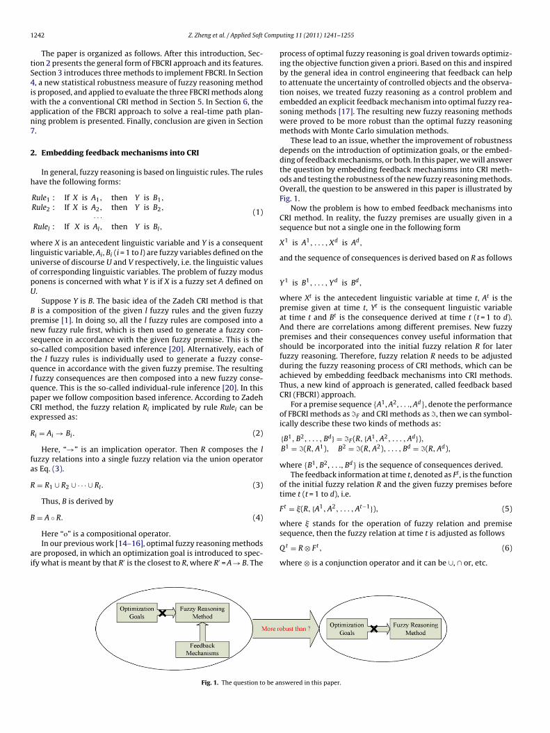
dx.doi.org/10.1016/j.asoc.2010.03.001

http://www.sciencedirect.com/science/journal/15684946

www.elsevier.com/locate/asoc

mailto:[email protected]

mailto:[email protected]

dx.doi.org/10.1016/j.asoc.2010.03.001

1 Comp

tS4iwan7

2

h

wluopU

BpnsstqlqpCe

R

fa

R

B

ai

242 Z. Zheng et al. / Applied Soft

The paper is organized as follows. After this introduction, Sec-ion 2 presents the general form of FBCRI approach and its features.ection 3 introduces three methods to implement FBCRI. In Section, a new statistical robustness measure of fuzzy reasoning method

s proposed, and applied to evaluate the three FBCRI methods alongith the a conventional CRI method in Section 5. In Section 6, the

pplication of the FBCRI approach to solve a real-time path plan-ing problem is presented. Finally, conclusion are given in Section.

. Embedding feedback mechanisms into CRI

In general, fuzzy reasoning is based on linguistic rules. The rulesave the following forms:

Rule1 : If X is A1, then Y is B1,Rule2 : If X is A2, then Y is B2,

· · ·Rulel : If X is Al, then Y is Bl,

(1)

here X is an antecedent linguistic variable and Y is a consequentinguistic variable, Ai, Bi (i = 1 to l) are fuzzy variables defined on theniverse of discourse U and V respectively, i.e. the linguistic valuesf corresponding linguistic variables. The problem of fuzzy modusonens is concerned with what Y is if X is a fuzzy set A defined on.

Suppose Y is B. The basic idea of the Zadeh CRI method is thatis a composition of the given l fuzzy rules and the given fuzzy

remise [1]. In doing so, all the l fuzzy rules are composed into aew fuzzy rule first, which is then used to generate a fuzzy con-equence in accordance with the given fuzzy premise. This is theo-called composition based inference [20]. Alternatively, each ofhe l fuzzy rules is individually used to generate a fuzzy conse-uence in accordance with the given fuzzy premise. The resultingfuzzy consequences are then composed into a new fuzzy conse-uence. This is the so-called individual-rule inference [20]. In thisaper we follow composition based inference. According to ZadehRI method, the fuzzy relation Ri implicated by rule Rulei can bexpressed as:

i = Ai → Bi. (2)

Here, “→” is an implication operator. Then R composes the luzzy relations into a single fuzzy relation via the union operators Eq. (3).

= R1 ∪ R2 ∪ · · · ∪ Rl. (3)

Thus, B is derived by

= A ◦ R. (4)

Here “о” is a compositional operator.In our previous work [14–16], optimal fuzzy reasoning methods

re proposed, in which an optimization goal is introduced to spec-fy what is meant by that R′ is the closest to R, where R′ = A → B. The

Fig. 1. The question to be an

uting 11 (2011) 1241–1255

process of optimal fuzzy reasoning is goal driven towards optimiz-ing the objective function given a priori. Based on this and inspiredby the general idea in control engineering that feedback can helpto attenuate the uncertainty of controlled objects and the observa-tion noises, we treated fuzzy reasoning as a control problem andembedded an explicit feedback mechanism into optimal fuzzy rea-soning methods [17]. The resulting new fuzzy reasoning methodswere proved to be more robust than the optimal fuzzy reasoningmethods with Monte Carlo simulation methods.

These lead to an issue, whether the improvement of robustnessdepends on the introduction of optimization goals, or the embed-ding of feedback mechanisms, or both. In this paper, we will answerthe question by embedding feedback mechanisms into CRI meth-ods and testing the robustness of the new fuzzy reasoning methods.Overall, the question to be answered in this paper is illustrated byFig. 1.

Now the problem is how to embed feedback mechanisms intoCRI method. In reality, the fuzzy premises are usually given in asequence but not a single one in the following form

X1 is A1, . . . , Xd is Ad,

and the sequence of consequences is derived based on R as follows

Y1 is B1, . . . , Yd is Bd,

where Xt is the antecedent linguistic variable at time t, At is thepremise given at time t, Yt is the consequent linguistic variableat time t and Bt is the consequence derived at time t (t = 1 to d).And there are correlations among different premises. New fuzzypremises and their consequences convey useful information thatshould be incorporated into the initial fuzzy relation R for laterfuzzy reasoning. Therefore, fuzzy relation R needs to be adjustedduring the fuzzy reasoning process of CRI methods, which can beachieved by embedding feedback mechanisms into CRI methods.Thus, a new kind of approach is generated, called feedback basedCRI (FBCRI) approach.

For a premise sequence {A1, A2, . . ., Ad}, denote the performanceof FBCRI methods as �F and CRI methods as �, then we can symbol-ically describe these two kinds of methods as:

{B1, B2, . . . , Bd} = �F (R, {A1, A2, . . . , Ad}),B1 = �(R,A1), B2 = �(R,A2), . . . , Bd = �(R,Ad),

where {B1, B2, . . ., Bd} is the sequence of consequences derived.The feedback information at time t, denoted as Ft, is the function

of the initial fuzzy relation R and the given fuzzy premises beforetime t (t = 1 to d), i.e.

Ft = �(R, {A1, A2, . . . , At−1}), (5)

where � stands for the operation of fuzzy relation and premisesequence, then the fuzzy relation at time t is adjusted as follows

Qt = R⊗ Ft, (6)

where ⊗ is a conjunction operator and it can be ∪, ∩ or, etc.

swered in this paper.

Z. Zheng et al. / Applied Soft Comp

B

Ca

B

SS

E

3

otmigc

1 1

Fig. 2. Diagram for CRI approach.

Thus, Bt is derived by

t = At ◦ Qt. (7)

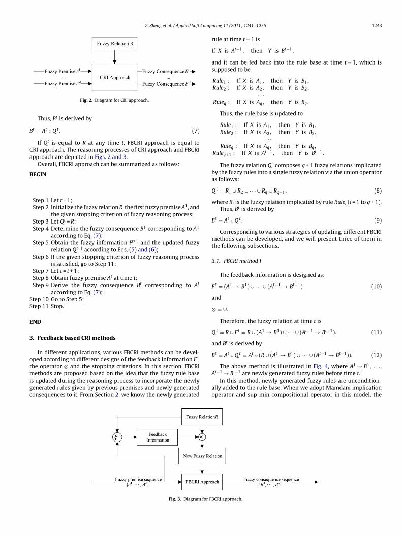
If Qt is equal to R at any time t, FBCRI approach is equal toRI approach. The reasoning processes of CRI approach and FBCRIpproach are depicted in Figs. 2 and 3.

Overall, FBCRI approach can be summarized as follows:

EGIN

Step 1 Let t = 1;Step 2 Initialize the fuzzy relation R, the first fuzzy premise A1, and

the given stopping criterion of fuzzy reasoning process;Step 3 Let Qt = R;Step 4 Determine the fuzzy consequence B1 corresponding to A1

according to Eq. (7);Step 5 Obtain the fuzzy information Ft+1 and the updated fuzzy

relation Qt+1 according to Eqs. (5) and (6);Step 6 If the given stopping criterion of fuzzy reasoning process

is satisfied, go to Step 11;Step 7 Let t = t + 1;Step 8 Obtain fuzzy premise At at time t;Step 9 Derive the fuzzy consequence Bt corresponding to At

according to Eq. (7);tep 10 Go to Step 5;tep 11 Stop.

ND

. Feedback based CRI methods

In different applications, various FBCRI methods can be devel-ped according to different designs of the feedback information Ft,
he operator ⊗ and the stopping criterions. In this section, FBCRI
ethods are proposed based on the idea that the fuzzy rule bases updated during the reasoning process to incorporate the newlyenerated rules given by previous premises and newly generatedonsequences to it. From Section 2, we know the newly generated

Fig. 3. Diagram for FB

uting 11 (2011) 1241–1255 1243

rule at time t − 1 is

If X is At−1, then Y is Bt−1,

and it can be fed back into the rule base at time t − 1, which issupposed to be


· · ·Ruleq : If X is Aq, then Y is Bq.

Thus, the rule base is updated to


· · ·Ruleq : If X is Aq, then Y is Bq,

Ruleq+1 : If X is At−1, then Y is Bt−1.

The fuzzy relation Qt composes q + 1 fuzzy relations implicatedby the fuzzy rules into a single fuzzy relation via the union operatoras follows:

Qt = R1 ∪ R2 ∪ · · · ∪ Rq ∪ Rq+1, (8)

where Ri is the fuzzy relation implicated by rule Rulei (i = 1 to q + 1).Thus, Bt is derived by

Bt = At ◦ Qt. (9)

Corresponding to various strategies of updating, different FBCRImethods can be developed, and we will present three of them inthe following subsections.

3.1. FBCRI method I

The feedback information is designed as:

Ft = (A1 → B1) ∪ · · · ∪ (At−1 → Bt−1) (10)

and

⊗ = ∪.Therefore, the fuzzy relation at time t is

Qt = R ∪ Ft = R ∪ (A1 → B1) ∪ · · · ∪ (At−1 → Bt−1), (11)

and Bt is derived by

Bt = At ◦ Qt = At ◦ (R ∪ (A1 → B1) ∪ · · · ∪ (At−1 → Bt−1)). (12)

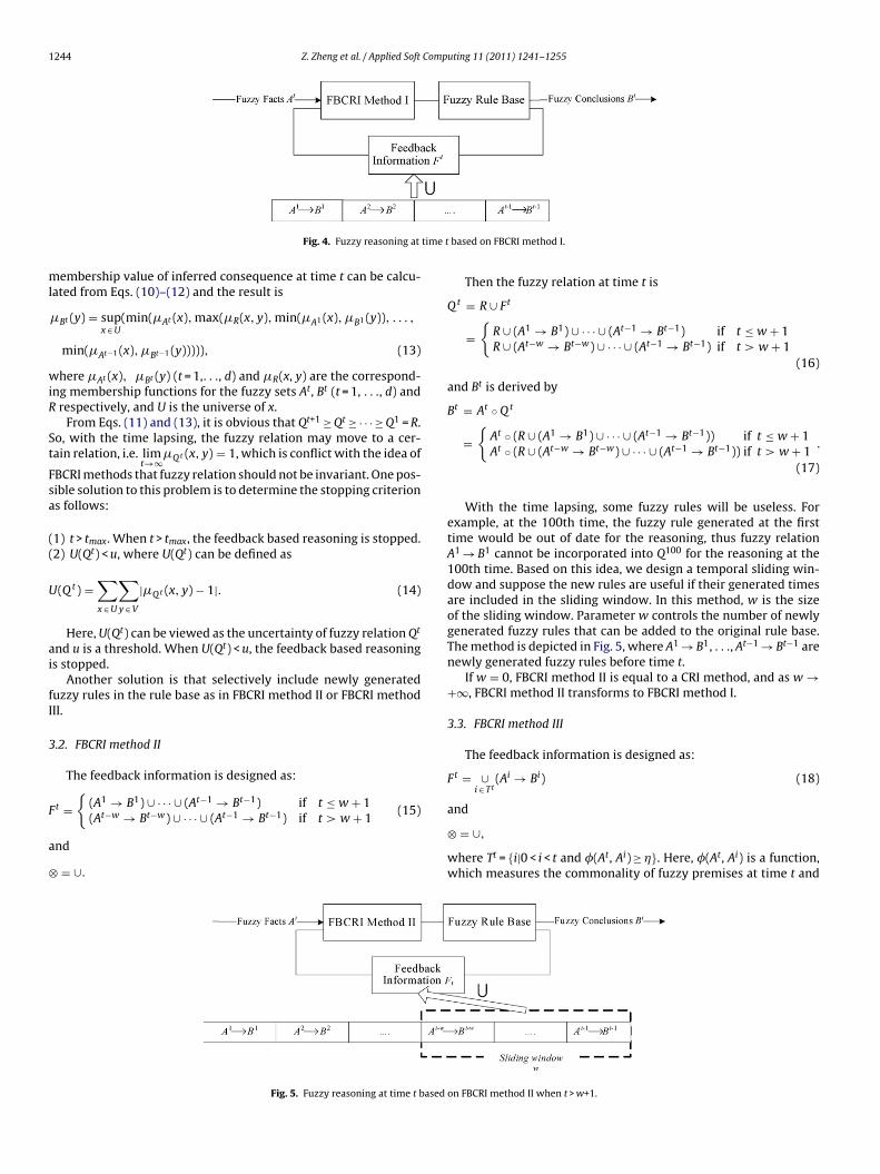
The above method is illustrated in Fig. 4, where A → B , . . .,At−1 → Bt−1 are newly generated fuzzy rules before time t.

In this method, newly generated fuzzy rules are uncondition-ally added to the rule base. When we adopt Mamdani implicationoperator and sup-min compositional operator in this model, the

CRI approach.

1244 Z. Zheng et al. / Applied Soft Computing 11 (2011) 1241–1255

time t

ml

wiR

St

Fsa

((

U

ai

fI

3

F

a

⊗

Fig. 4. Fuzzy reasoning at

embership value of inferred consequence at time t can be calcu-ated from Eqs. (10)–(12) and the result is

�Bt (y) = supx∈U

(min(�At (x),max(�R(x, y),min(�A1 (x),�B1 (y)), . . . ,

min(�At−1 (x),�Bt−1 (y))))), (13)

here �At (x), �Bt (y) (t = 1,. . ., d) and �R(x, y) are the correspond-ng membership functions for the fuzzy sets At, Bt (t = 1, . . ., d) andrespectively, and U is the universe of x.

From Eqs. (11) and (13), it is obvious that Qt+1 ≥ Qt ≥ · · · ≥ Q1 = R.o, with the time lapsing, the fuzzy relation may move to a cer-ain relation, i.e. lim

t→∞�Qt (x, y) = 1, which is conflict with the idea of

BCRI methods that fuzzy relation should not be invariant. One pos-ible solution to this problem is to determine the stopping criterions follows:

1) t > tmax. When t > tmax, the feedback based reasoning is stopped.2) U(Qt) < u, where U(Qt) can be defined as

(Qt) =∑x∈U

∑y∈V

|�Qt (x, y) − 1|. (14)

Here, U(Qt) can be viewed as the uncertainty of fuzzy relation Qt

nd u is a threshold. When U(Qt) < u, the feedback based reasonings stopped.

Another solution is that selectively include newly generateduzzy rules in the rule base as in FBCRI method II or FBCRI methodII.

.2. FBCRI method II

The feedback information is designed as:{(A1 → B1) ∪ · · · ∪ (At−1 → Bt−1) if t ≤ w + 1
t =(At−w → Bt−w) ∪ · · · ∪ (At−1 → Bt−1) if t > w + 1
(15)

nd

= ∪.

Fig. 5. Fuzzy reasoning at time t based

based on FBCRI method I.

Then the fuzzy relation at time t is

Qt = R ∪ Ft

={R ∪ (A1 → B1) ∪ · · · ∪ (At−1 → Bt−1) if t ≤ w + 1R ∪ (At−w → Bt−w) ∪ · · · ∪ (At−1 → Bt−1) if t > w + 1

(16)

and Bt is derived by

Bt = At ◦ Qt

={At ◦ (R ∪ (A1 → B1) ∪ · · · ∪ (At−1 → Bt−1)) if t ≤ w + 1At ◦ (R ∪ (At−w → Bt−w) ∪ · · · ∪ (At−1 → Bt−1)) if t > w + 1

.

(17)

With the time lapsing, some fuzzy rules will be useless. Forexample, at the 100th time, the fuzzy rule generated at the firsttime would be out of date for the reasoning, thus fuzzy relationA1 → B1 cannot be incorporated into Q100 for the reasoning at the100th time. Based on this idea, we design a temporal sliding win-dow and suppose the new rules are useful if their generated timesare included in the sliding window. In this method, w is the sizeof the sliding window. Parameter w controls the number of newlygenerated fuzzy rules that can be added to the original rule base.The method is depicted in Fig. 5, where A1 → B1, . . ., At−1 → Bt−1 arenewly generated fuzzy rules before time t.

If w = 0, FBCRI method II is equal to a CRI method, and as w →+∞, FBCRI method II transforms to FBCRI method I.

3.3. FBCRI method III

The feedback information is designed as:

Ft = ∪i∈ Tt

(Ai → Bi) (18)

and

⊗ = ∪,where Tt = {i|0 < i < t and �(At, Ai) ≥�}. Here, �(At, Ai) is a function,which measures the commonality of fuzzy premises at time t and

on FBCRI method II when t > w+1.

Comp

tvb

Q

B

mrtaAtb

i

psm

ektA

�

w√t

4

cadsdoTocm

tds

max

Z. Zheng et al. / Applied Soft

ime i. If the commonality degree is not smaller than a constantalue �, the newly generated rule Rulei (0 < i < t) is added to rulease RBt and contributes to the fuzzy reasoning at time t.

Then the fuzzy relation at time t is

t = R ∪ Ft = R ∪(⋃i∈ Tt

(Ai → Bi)

). (19)

Thus, Bt is derived by

t = At ◦ Qt = At ◦(R ∪(⋃i∈ Tt

(Ai → Bi)

)). (20)

The basic idea of the method is that, if a previous premise is com-on enough with the premise at time t, its related new generated

ule should contribute “suggestions” for the fuzzy reasoning at time. Based on this, the commonality measure of the new fuzzy premisend the existing premises is included in the feedback mechanism.newly generated rule can be added to the rule base if and only if

he commonality degree between its premise and the premise toe processed is higher than �.

Note, as �→ +∞, FBCRI method III is equal to a CRI method, andf �≤ 0, FBCRI method III transforms to FBCRI method I.

In Sections 5 and 6, we will apply the commonality measureroposed in [21] to the robustness comparison analysis and theolution of a real-time path planning problem. The commonalityeasure gauges the amount of common information that may

xist between two fuzzy sets [21]. It uses the concept of specificnowledge that is shared between two distinct pieces of informa-ion sources. In the reference, the commonality of two fuzzy sets1 and A2 are measured by the equation

(A1, A2) = 1 − e−Sp(C)/d(A1,A2), (21)

here C = A1 ∩ A2 and Sp(C) is the specificity [22] of C. d(A1, A2) =∑x∈U(�A1 (x) −�A2 (x))2 is the distance between A1 and A2. If

he two fuzzy premises are same, i.e. A1 = A2, then �(A2, A1) = 1.

. Robustness measure

Informally, fuzzy reasoning method can be viewed as a pro-ess by which a possible imprecise consequence is deduced fromcollection of imprecise premises [23]. The imprecision can be

escribed by linguistic variables and the collection is the set ofome linguistic rules. A good result of fuzzy reasoning not onlyepends on the design of linguistic variables and the constructionf the rules, but also depends on the fuzzy reasoning method used.herefore, a discussion for comparison of fuzzy reasoning meth-ds is needed. In this section, robustness is used as the criterion ofomparing fuzzy reasoning methods, especially the proposed FBCRI

RM =d∑t=1

(RMt) =d∑t=1

⎛⎜⎜⎝sup

y

⎛⎜⎜⎝

ethods and conventional CRI methods.We hope that an FBCRI method can have the property, that is,

he consequences Bt and B′t should be similar when the premise A′t

eviates slightly from At or the original fuzzy relation R′ deviateslightly from R due to system noises or parameter perturbations.

uting 11 (2011) 1241–1255 1245

The property is concerned with the robustness problem of fuzzyreasoning, which is discussed in this paper.

An FBCRI method determines consequences of a given sequenceof fuzzy premises based on given fuzzy rules and the newly gener-ated rules. The given rules are usually combined to make up a fuzzyrelation and the newly generated rules are determined by the fuzzyrelation and the given premises. So, the robustness measure RM ofan FBCRI method should be a function of the given fuzzy relationand the given sequence of fuzzy premises:

RM =M(R, {A1, . . . , Ad}).

A natural method to evaluate the function M is to define andderive M analytically, as shown in [14,15] by using the so-calledı-equalities of fuzzy sets. However, ı-equalities of fuzzy sets canbe used as an analysis tool but not a comparing tool of robustness,because the robustness results in terms of ı-equalities are conser-vative in certain sense and we can not obtain the maximum of ıthat ensures the corresponding ı-equality hold. Alternatively, in[15,17], the function of M is evaluated by the popular Monte Carlosimulation methods. Similar to [15,17], the robustness is also mea-sured with Monte Carlo simulation methods in our work. We willelaborate on it later.

First we present the definition of the robustness of FBCRI meth-ods. Suppose the perturbations related to R and At (1 ≤ t ≤ d) are�Rand �At, and let R′ = R +�R and A′t = At +�At (1 ≤ t ≤ d), then thesequence of fuzzy consequences {B′1, . . . , B′d} can be derived fromR′ and {A′1, . . . , A′d}.Definition 1. (Robustness of FBCRI Methods): The robustness ofan FBCRI method is defined as

|�B′t (y) −�Bt (y)|(supx

(�A′t (x) −�At (x)), supx

(�R′ (x, y) −�R(x, y))

)⎞⎟⎟⎠⎞⎟⎟⎠ , (22)

where �Bt (y) and �B′t (y) (t = 1, . . ., d) are the corresponding mem-bership functions for the fuzzy sets Bt and B′t (t = 1, . . ., d), �R(x, y)and �R′ (x, y) are the corresponding membership functions for thefuzzy sets R and R′, and V is the universe of discourses.

The robustness measure calculated in Def. 1 is similar to that in[17]. It takes account of errors in the resulting fuzzy consequencesas well as their causing errors in fuzzy premises and fuzzy relations.Formula max(sup

x(�A′t (x) −�At (x)), sup

x(�R′ (x, y) −�R(x, y))) is

the maximal causing error of�Bt (y). The robustness measure lookslike a measure of partial difference. This is different from the robust-ness measure introduced in [15] that only considers errors in theresulting fuzzy consequences and ignores their causing errors infuzzy premises and relations. The difference between the measurepresented here and that in [17] is that the three measures underdifferent cases in [17] are combined to form a single measure inthis paper.

It is easy to derive from Def.1 that the less the value calculated byEq. (22), the better the robustness of an FBCRI method. The theoret-ical analysis of RM is very complicated, so we use the popular MonteCarlo simulation method to estimate its value. In the simulations,we assume that:

(1) Methods 1–4 represent FBCRI method I, FBCRI method II, FBCRI
method III, CRI method, respectively.
(2) We only consider the case of finite discrete universes withU = {u1, . . ., um} and V = {v1, . . . , vn}.

(3) For R = [rij]m×n and the sequence {A1 = [a1i]1×m, . . . , A

d =[adi]1×m}, where rij ∈ [0,1], a1

i, . . . , ad

i∈ [0,1] (i = 1, . . ., m; j = 1,

1 Comp

(

1, . . .

1, . .

(

Mf

S

S

S

S

ordbtAfrawr

S

S

S

S

experiment also verifies the analysis in Section 3.2.(3) FBCRI method I is more robust than the CRI method.(4) FBCRI method II is more robust than CRI method under all sizes

of sliding windows except for w = 0.


. . ., n), the corresponding sequence of consequences is {B1 =[b1i]1×n, . . . , B

d = [bdi]1×n}.

4) �R = [�rij]m×n, �A1 = [�a1i]1×m, . . . ,�A

d = [�adi]1×m

are the perturbations of R and A1, . . ., Ad respectively,and �rij,�a

1i, . . . ,�ad

iare normally distributed ran-

dom variables in accordance with the distribution N(0,1) and in the interval (−0.025, 0.025). Let R′ = R +�R, andA′1 = A1 +�A1, . . . , A′d = Ad +�Ad, where

r′ij

={

1 rij +�rij ∈ (1,+∞)rij +�rij rij +�rij ∈ [0,1]0 rij +�rij ∈ (−∞,0)

i = 1, . . . ,m and j =

a′qi

={

1 aqi

+�aqi∈ (1,+∞)

aqi

+�aqiaqi

+�aqi∈ [0,1]

0 aqi

+�aqi∈ (−∞,0)

i = 1, . . . ,m and q =

5) For R′ = [r′ij]m×n and the sequence {A′1 = [a′1

i ]1×m, . . . , A′d =

[a′di ]1×m}, the corresponding sequence of consequences is {B′1 =

[b′1i ]1×n, . . . , B

′t = [b′di ]1×n}.

For the given R and the premises sequence {A1, . . ., Ad}, theonte Carlo simulation for method k (k = 1 to 4) can be done as

ollows:

imulation Algorithm 1

tep 1 Obtain the fuzzy consequences {B1, . . ., Bd} corresponding to thefuzzy premises {A1, . . ., Ad} with method k. If k = 2, the size of slidingwindow w should be initialized;

tep 2 Suppose p is the number of perturbations.For e = 1 to p

Step 2.1: Randomly generate the perturbations {�rij , i = 1 to m andj = 1 to n} and {�aq

i, i = 1 to m and q = 1 to d}, then R′ and the sequence

{A′1, . . . , A′d} can be calculated;Step 2.2: Obtain the fuzzy consequences {B′1, . . . , B′d}

corresponding to the fuzzy premises {A′1, . . . , A′d} based on R′ withmethod k;

Step 2.3: Calculate RMek

according to Def. 1, where RMek

is therobustness of method k in trail e;

tep 3 Stop.Simulation algorithm 1 is actually conducted for p trials, each

f which generate a value RMek

for measuring robustness of fuzzyeasoning. However, the robustness calculated in Step 2.3 isefined for a given pair of R and {A1, . . ., Ad}, considering pertur-ations of fuzzy premises only. Obviously, this is not sufficiento evaluate the robustness of a given fuzzy reasoning method.

better robustness measure should be a function of the givenuzzy reasoning method only and is irrelevant of specific fuzzyelations and fuzzy premises. As a result, we have the followinglgorithm with f trials of simulation conducted. And, in this way,e can employ the following algorithm to evaluate and compare

obustness of the four methods against perturbations.

imulation Algorithm 2

tep 1 Generate f groups of fuzzy relations and sequences of fuzzypremises 〈R(s), {A1

(s), . . . , Ad

(s)}〉, s = 1, 2, . . ., f. For each s, the memberships

are all generated in accordance with the uniform probability distributiondefined over the interval [0, 1];

tep 2 For each group 〈R(s), {A1(s), . . . , Ad

(s)}〉, perform Simulation Algorithm

1 for method 1, 2, 3, 4 and obtain RMek(s)

(k = 1 to 4) for the sth pair offuzzy relation and sequence of fuzzy premises in the eth perturbation.

tep 3 For method i (i ∈ {1, 2, 3}), calculate

uting 11 (2011) 1241–1255

, n

. , d

. (23)

RMi =∑f

s=1

∑pe=1RM

ei(s)

p× q . (24)

Step 4 Stop.

5. Robustness comparison analysis

Based on the robustness measure defined in Section 4, therobustness comparison of the four methods will be analyzed from

three categories. For FBCRI method III, the commonality of fuzzypremises is measured by Eq. (21). Note, when the constant value �in FBCRI method III is set to be smaller than 0.6, there are no muchdifference between FBCRI method I and FBCRI method III. Therefore,� is set to be 0.6.

5.1. Robustness comparison analysis I

The first category considers�R only and ignores�At (t = 1 to d),that is�R /= 0, and�At = 0 (t = 1 to d).

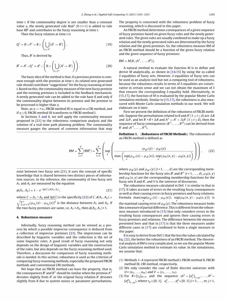
Example 1. Let m = n = 7, d = 50, p = 1000, f = 100. And Mamdaniimplication operator and sup-min compositional operator are used.As w moving from 1 to 50, the changing of the robustness of thefour methods is illustrated in Fig. 6. Note, although the robustnessof FBCRI method I, FBCRI method III and CRI method is unrelated tosliding window sizes, we paint them on figures for clear compari-son.

From Fig. 6, we can conclude that

(1) In the case w = 0, the robustness of FBCRI method II is equalto that of the CRI method. The reason is that FBCRI method IIand the CRI method are equivalent under this condition. Theexperiment verifies the analysis in Section 3.2.

(2) In the case w = 50, the robustness of FBCRI method II is equalto that of FBCRI method I. The reason is that FBCRI method IIand FBCRI method I are equivalent under this condition. The

Fig. 6. Comparison of the four methods in the case�R /= 0, and�At = 0.

Z. Zheng et al. / Applied Soft Computing 11 (2011) 1241–1255 1247

(

(

5

�

EiAm

(

(

((

(

5

�

Ecwm

(

(

((

(

are the turn angle values recommended by PS behavior and GS

Fig. 7. Comparison of the four methods in the case�R = 0, and�At /= 0.

5) When w /= 0, FBCRI method II is at least as robust as FBCRImethod I. Whenw is close to d, the robustness of the two meth-ods is same, because in this case, FBCRI method II is almostequivalent to FBCRI method I.

6) FBCRI method III is more robust than CRI method, but it is lessrobust than FBCRI method I.

.2. Robustness comparison analysis II

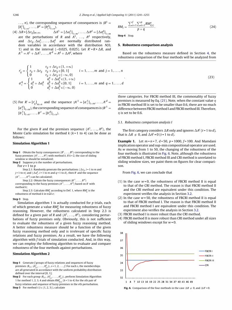
The second category only considers�At (t = 1 to d) and ignoresR, that is�R = 0, and�At /= 0 (t = 1 to d).

xample 2. Let m = n = 7, d = 50, p = 1000, f = 100. And Mamdanimplication operator and sup-min compositional operator are used.swmoving from 1 to 50, the changing of the robustness of the fourethods is illustrated in Fig. 7.


1) In the casew = 0, the robustness of FBCRI method II is equal tothat of the CRI method.

2) In the case w = 50, the robustness of FBCRI method II is equalto that of FBCRI method I.

3) FBCRI method I is more robust than the CRI method.4) FBCRI method II is more robust than the CRI method except for

the case with w = 0.5) Though FBCRI method III is more robust than the CRI method,

it is less robust than FBCRI method I.

.3. Robustness comparison analysis III

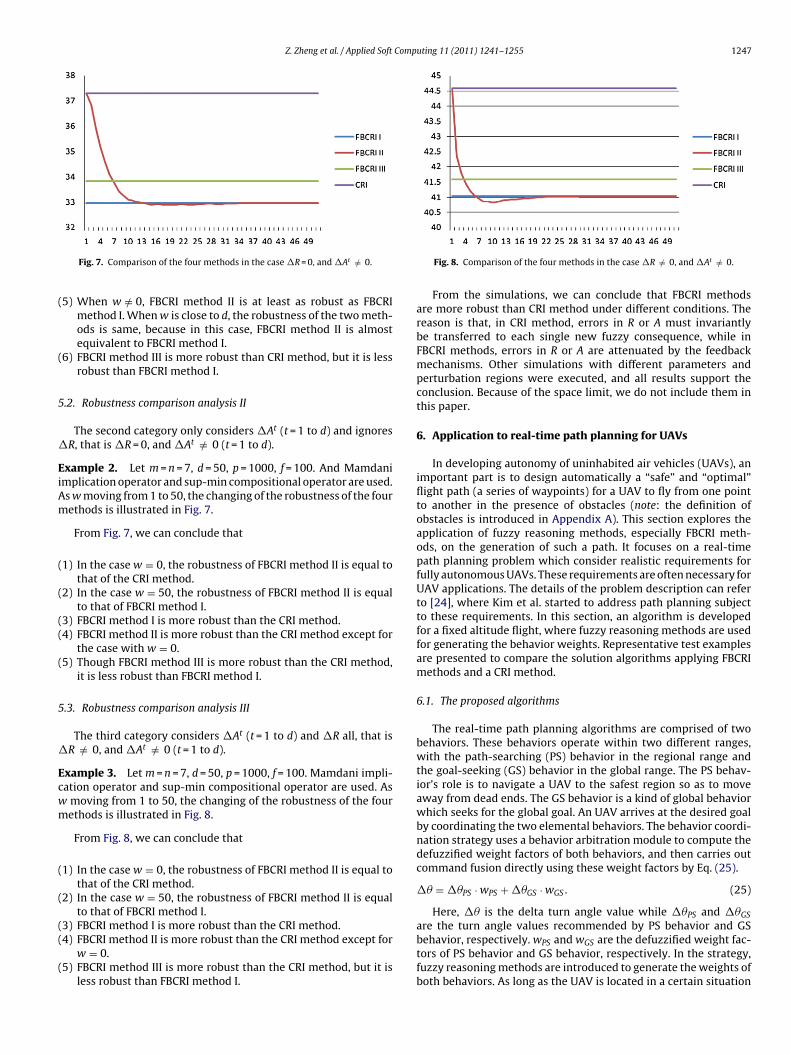
The third category considers �At (t = 1 to d) and �R all, that isR /= 0, and�At /= 0 (t = 1 to d).

xample 3. Let m = n = 7, d = 50, p = 1000, f = 100. Mamdani impli-ation operator and sup-min compositional operator are used. As

moving from 1 to 50, the changing of the robustness of the fourethods is illustrated in Fig. 8.


1) In the casew = 0, the robustness of FBCRI method II is equal tothat of the CRI method.

2) In the case w = 50, the robustness of FBCRI method II is equalto that of FBCRI method I.

3) FBCRI method I is more robust than the CRI method.
4) FBCRI method II is more robust than the CRI method except forw = 0.
5) FBCRI method III is more robust than the CRI method, but it isless robust than FBCRI method I.

Fig. 8. Comparison of the four methods in the case�R /= 0, and�At /= 0.

From the simulations, we can conclude that FBCRI methodsare more robust than CRI method under different conditions. Thereason is that, in CRI method, errors in R or A must invariantlybe transferred to each single new fuzzy consequence, while inFBCRI methods, errors in R or A are attenuated by the feedbackmechanisms. Other simulations with different parameters andperturbation regions were executed, and all results support theconclusion. Because of the space limit, we do not include them inthis paper.

6. Application to real-time path planning for UAVs

In developing autonomy of uninhabited air vehicles (UAVs), animportant part is to design automatically a “safe” and “optimal”flight path (a series of waypoints) for a UAV to fly from one pointto another in the presence of obstacles (note: the definition ofobstacles is introduced in Appendix A). This section explores theapplication of fuzzy reasoning methods, especially FBCRI meth-ods, on the generation of such a path. It focuses on a real-timepath planning problem which consider realistic requirements forfully autonomous UAVs. These requirements are often necessary forUAV applications. The details of the problem description can referto [24], where Kim et al. started to address path planning subjectto these requirements. In this section, an algorithm is developedfor a fixed altitude flight, where fuzzy reasoning methods are usedfor generating the behavior weights. Representative test examplesare presented to compare the solution algorithms applying FBCRImethods and a CRI method.

6.1. The proposed algorithms

The real-time path planning algorithms are comprised of twobehaviors. These behaviors operate within two different ranges,with the path-searching (PS) behavior in the regional range andthe goal-seeking (GS) behavior in the global range. The PS behav-ior’s role is to navigate a UAV to the safest region so as to moveaway from dead ends. The GS behavior is a kind of global behaviorwhich seeks for the global goal. An UAV arrives at the desired goalby coordinating the two elemental behaviors. The behavior coordi-nation strategy uses a behavior arbitration module to compute thedefuzzified weight factors of both behaviors, and then carries outcommand fusion directly using these weight factors by Eq. (25).

�� =��PS ·wPS +��GS ·wGS. (25)

Here, �� is the delta turn angle value while ��PS and ��GS

behavior, respectively.wPS andwGS are the defuzzified weight fac-tors of PS behavior and GS behavior, respectively. In the strategy,fuzzy reasoning methods are introduced to generate the weights ofboth behaviors. As long as the UAV is located in a certain situation


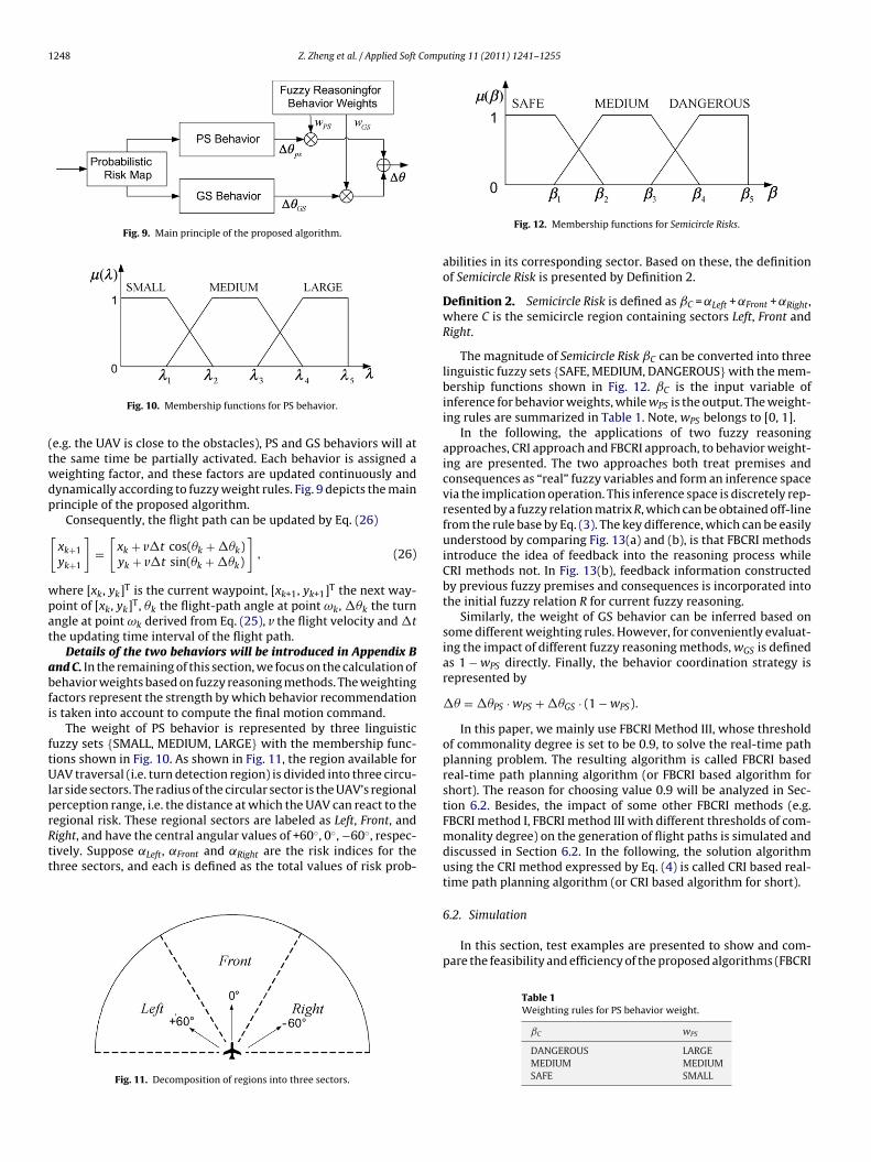
Fig. 9. Main principle of the proposed algorithm.

(twdp

[

wpat

abfi

ftUlprRtt

Fig. 10. Membership functions for PS behavior.

e.g. the UAV is close to the obstacles), PS and GS behaviors will athe same time be partially activated. Each behavior is assigned aeighting factor, and these factors are updated continuously andynamically according to fuzzy weight rules. Fig. 9 depicts the mainrinciple of the proposed algorithm.

Consequently, the flight path can be updated by Eq. (26)

xk+1yk+1

]=[xk + v�t cos(�k +��k)yk + v�t sin(�k +��k)

], (26)

here [xk, yk]T is the current waypoint, [xk+1, yk+1]T the next way-oint of [xk, yk]T, �k the flight-path angle at point ωk,��k the turnngle at point ωk derived from Eq. (25), v the flight velocity and�the updating time interval of the flight path.

Details of the two behaviors will be introduced in Appendix Bnd C. In the remaining of this section, we focus on the calculation ofehavior weights based on fuzzy reasoning methods. The weightingactors represent the strength by which behavior recommendations taken into account to compute the final motion command.

The weight of PS behavior is represented by three linguisticuzzy sets {SMALL, MEDIUM, LARGE} with the membership func-ions shown in Fig. 10. As shown in Fig. 11, the region available forAV traversal (i.e. turn detection region) is divided into three circu-

ar side sectors. The radius of the circular sector is the UAV’s regionalerception range, i.e. the distance at which the UAV can react to the
egional risk. These regional sectors are labeled as Left, Front, andight, and have the central angular values of +60◦, 0◦, −60◦, respec-ively. Suppose ˛Left, ˛Front and ˛Right are the risk indices for thehree sectors, and each is defined as the total values of risk prob-
Fig. 11. Decomposition of regions into three sectors.

Fig. 12. Membership functions for Semicircle Risks.

abilities in its corresponding sector. Based on these, the definitionof Semicircle Risk is presented by Definition 2.

Definition 2. Semicircle Risk is defined as ˇC =˛Left +˛Front +˛Right,where C is the semicircle region containing sectors Left, Front andRight.

The magnitude of Semicircle Risk ˇC can be converted into threelinguistic fuzzy sets {SAFE, MEDIUM, DANGEROUS} with the mem-bership functions shown in Fig. 12. ˇC is the input variable ofinference for behavior weights, whilewPS is the output. The weight-ing rules are summarized in Table 1. Note, wPS belongs to [0, 1].

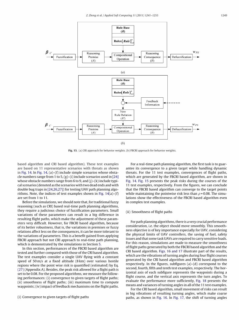
In the following, the applications of two fuzzy reasoningapproaches, CRI approach and FBCRI approach, to behavior weight-ing are presented. The two approaches both treat premises andconsequences as “real” fuzzy variables and form an inference spacevia the implication operation. This inference space is discretely rep-resented by a fuzzy relation matrix R, which can be obtained off-linefrom the rule base by Eq. (3). The key difference, which can be easilyunderstood by comparing Fig. 13(a) and (b), is that FBCRI methodsintroduce the idea of feedback into the reasoning process whileCRI methods not. In Fig. 13(b), feedback information constructedby previous fuzzy premises and consequences is incorporated intothe initial fuzzy relation R for current fuzzy reasoning.

Similarly, the weight of GS behavior can be inferred based onsome different weighting rules. However, for conveniently evaluat-ing the impact of different fuzzy reasoning methods,wGS is definedas 1 −wPS directly. Finally, the behavior coordination strategy isrepresented by

�� =��PS ·wPS +��GS · (1 −wPS).In this paper, we mainly use FBCRI Method III, whose threshold

of commonality degree is set to be 0.9, to solve the real-time pathplanning problem. The resulting algorithm is called FBCRI basedreal-time path planning algorithm (or FBCRI based algorithm forshort). The reason for choosing value 0.9 will be analyzed in Sec-tion 6.2. Besides, the impact of some other FBCRI methods (e.g.FBCRI method I, FBCRI method III with different thresholds of com-monality degree) on the generation of flight paths is simulated anddiscussed in Section 6.2. In the following, the solution algorithmusing the CRI method expressed by Eq. (4) is called CRI based real-time path planning algorithm (or CRI based algorithm for short).

6.2. Simulation

In this section, test examples are presented to show and com-pare the feasibility and efficiency of the proposed algorithms (FBCRI

Table 1Weighting rules for PS behavior weight.

ˇC wPS

DANGEROUS LARGEMEDIUM MEDIUMSAFE SMALL


ights.

baicwcdra

rtvreortFw

tTsr(si(w

(

Fig. 13. (a) CRI approach for behavior we

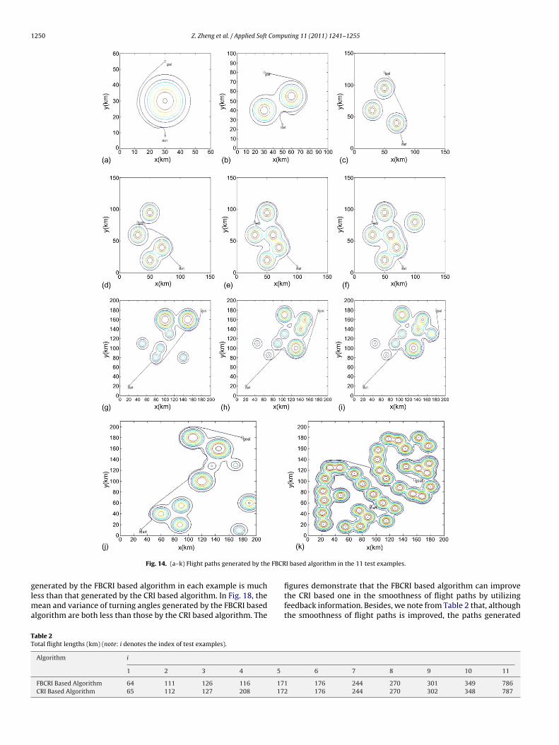
ased algorithm and CRI based algorithm). These test examplesre based on 11 representative scenarios with threats as shownn Fig. 14. In Fig. 14, (a)–(f) include simple scenarios whose obsta-le numbers range from 1 to 5, (g)–(i) include scenarios used in [24]hose obstacle numbers range from 6 to 9, and (j)–(k) include typi-

al scenarios (denoted as the scenarios with two dead ends and withouble bug traps in [24,26,27]) for testing UAV path planning algo-ithms. Note, the indices of test examples shown in Fig. 14(a)–(f)re set from 1 to 11.

Before the simulations, we should note that, for traditional fuzzyeasoning (such as CRI) based real-time path planning algorithms,hey require a judicious choice of fuzzification parameters. Smallariations of these parameters can result in a big difference inesulting flight paths, which make the adjustment of these param-ters very difficult. However, for FBCRI based algorithm, becausef its better robustness, that is, the variations in premises or fuzzyelations affect less on the consequences, it can be more tolerant tohe variations of parameters. This is a benefit gained from applyingBCRI approach but not CRI approach to real-time path planning,hich is demonstrated by the simulations in Section 5.

In this section, performances of the FBCRI based algorithm areested and further compared with those of the CRI based algorithm.he test examples consider a single UAV flying with a constantpeed of 50 m/s at a fixed altitude (8 km) over various hostileegions where the point wise risk is quantified (estimated) by Eq.27) (Appendix A). Besides, the peak risk allowed for a flight path iset to be 0.08. For the proposed algorithms, we measure the follow-ng performances: (i) convergence to given targets of flight paths;
ii) smoothness of flight paths; (iii) maximum time to computeaypoints; (iv) impact of feedback mechanisms on the flight paths.
i) Convergence to given targets of flight paths

(b) FBCRI approach for behavior weights.

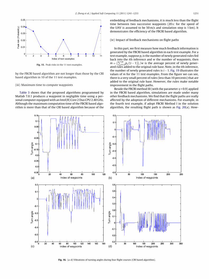
For a real-time path planning algorithm, the first task is to guar-antee its convergence to a given target while handling dynamicthreats. For the 11 test examples, convergences of flight paths,which are generated by the FBCRI based algorithm, are shown inFig. 14. Fig. 15 presents the peak risks during the courses of the11 test examples, respectively. From the figures, we can concludethat the FBCRI based algorithm can converge to the target pointswhile maintaining the pointwise risk less than = 0.08. The simu-lations show the effectiveness of the FBCRI based algorithm evenin complex test examples.

(ii) Smoothness of flight paths

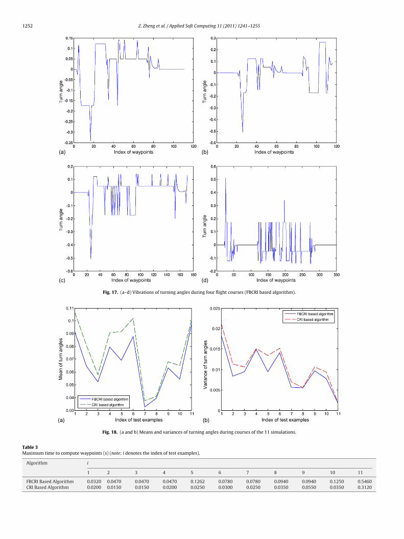
For path planning algorithms, there is a very crucial performanceconsideration, i.e. the object should move smoothly. This smooth-ness objective is of key importance especially for UAV, consideringthe physical limits of UAV controllers, the saving of fuel, safetyissues and that some task UAVs are required to carry sensitive loads.For this reason, simulations are made to measure the smoothnessof flight paths generated by both the FBCRI based algorithm and theCRI based algorithm. Figs. 16 and 17 illustrate part of the results,which are the vibrations of turning angles during four flight coursesgenerated by the CRI based algorithm and FBCRI based algorithmrespectively. In the figures, subfigures (a)–(d) correspond to thesecond, fourth, fifth and tenth test examples, respectively. The hor-izontal axis of each subfigure represents the waypoints during aflight course, and the vertical axis represents the turn angles. To
evaluate the performance more sufficiently, Fig. 18 presents themeans and variances of turning angles in all of the 11 test examples.
For the CRI based algorithm, small movement of risks can resultin big vibrations of resulting turning angles, which make coarsepaths, as shown in Fig. 16. In Fig. 17, the shift of turning angles


FBCR

glma

TT

Fig. 14. (a–k) Flight paths generated by the

enerated by the FBCRI based algorithm in each example is muchess than that generated by the CRI based algorithm. In Fig. 18, the

ean and variance of turning angles generated by the FBCRI basedlgorithm are both less than those by the CRI based algorithm. The

able 2otal flight lengths (km) (note: i denotes the index of test examples).

Algorithm i

1 2 3 4 5

FBCRI Based Algorithm 64 111 126 116 17CRI Based Algorithm 65 112 127 208 17

I based algorithm in the 11 test examples.

figures demonstrate that the FBCRI based algorithm can improvethe CRI based one in the smoothness of flight paths by utilizingfeedback information. Besides, we note from Table 2 that, althoughthe smoothness of flight paths is improved, the paths generated

6 7 8 9 10 11

1 176 244 270 301 349 7862 176 244 270 302 348 787


bb

(

MsAr

Fig. 15. Peak risks in the 11 test examples.

y the FBCRI based algorithm are not longer than those by the CRIased algorithm in 10 of the 11 test examples.

iii) Maximum time to compute waypoints

Table 3 shows that the proposed algorithms programmed byatlab 7.0.1 produces a waypoint in negligible time using a per-

onal computer equipped with an Intel(R) Core 2 Duo CPU 2.40 GHz.lthough the maximum computation time of the FBCRI based algo-ithm is more than that of the CRI based algorithm because of the

Fig. 16. (a–d) Vibrations of turning angles during

uting 11 (2011) 1241–1255 1251

embedding of feedback mechanisms, it is much less than the flighttime between two successive waypoints (20 s: for the speed ofthe UAV is assumed to be 50 m/s and simulation step is 1 km). Itdemonstrates the efficiency of the FBCRI based algorithm.

(iv) Impact of feedback mechanisms on flight paths

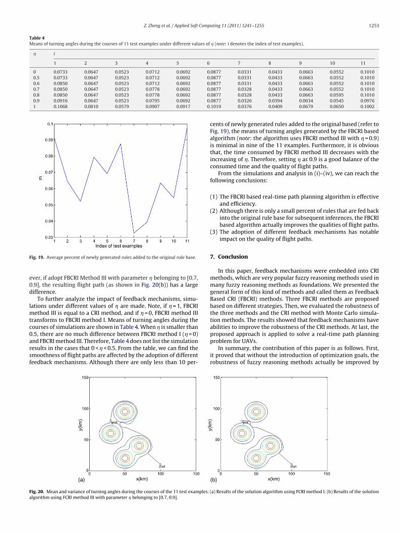
In this part, we first measure how much feedback information isgenerated by the FBCRI based algorithm in each test example. For atest example, suppose pi is the number of newly generated rules fedback into the ith inference and w the number of waypoints, thenm =

(∑wi=2pi/(i− 1)

)/w is the average percent of newly gener-

ated rules added to the original rule base. Note, in the ith inference,the number of newly generated rules is i − 1. Fig. 19 illustrates thevalues of m for the 11 test examples. From the figure we can see,there is a very small percent of rules (less than 10 percents) that areadded to the original rule base. However, the rules make notableimprovement in the flight paths.

Beside the FBCRI method III (with the parameter �= 0.9) applied
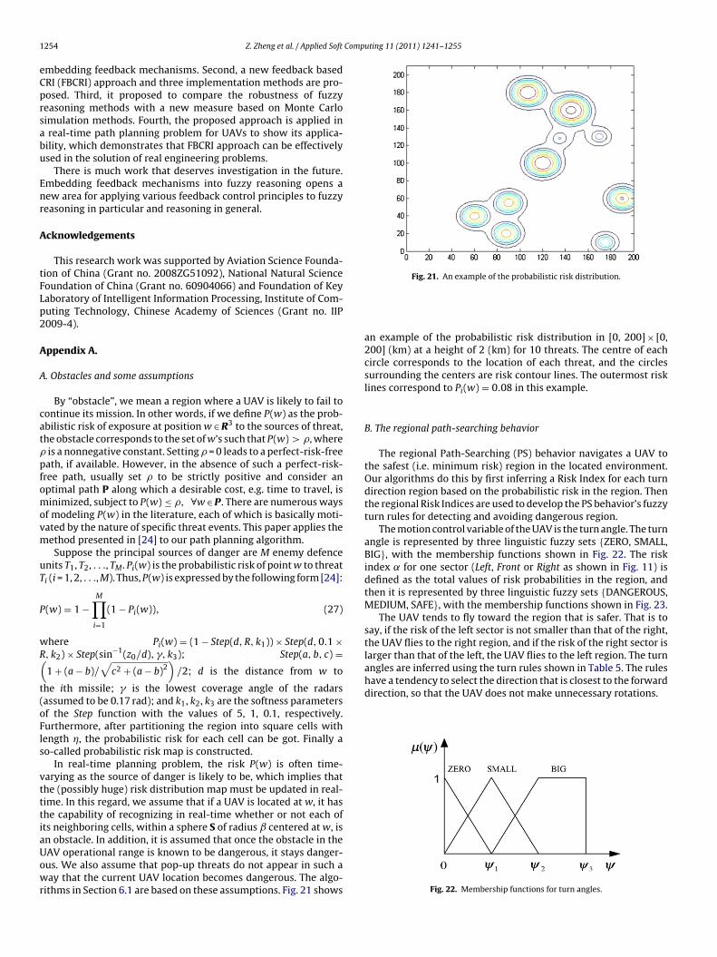
in the FBCRI based algorithm, simulations are made under manyother feedback mechanisms. We find that the flight paths are reallyaffected by the adoption of different mechanisms. For example, inthe fourth test example, if adopt FBCRI Method I in the solutionalgorithm, the resulting flight path is shown as Fig. 20(a). How-
four flight courses (CRI based algorithm).


Fig. 17. (a–d) Vibrations of turning angles during four flight courses (FBCRI based algorithm).

Fig. 18. (a and b) Means and variances of turning angles during courses of the 11 simulations.

Table 3Maximum time to compute waypoints (s) (note: i denotes the index of test examples).

Algorithm i

1 2 3 4 5

FBCRI Based Algorithm 0.0320 0.0470 0.0470 0.0470 0.1262CRI Based Algorithm 0.0200 0.0150 0.0150 0.0200 0.0250

6 7 8 9 10 11

0.0780 0.0780 0.0940 0.0940 0.1250 0.54600.0300 0.0250 0.0350 0.0550 0.0350 0.3120


Table 4Means of turning angles during the courses of 11 test examples under different values of � (note: i denotes the index of test examples).

� i

1 2 3 4 5 6 7 8 9 10 11

0 0.0733 0.0647 0.0523 0.0712 0.0692 0.0877 0.0331 0.0433 0.0663 0.0552 0.10100.5 0.0733 0.0647 0.0523 0.0712 0.0692 0.0877 0.0331 0.0433 0.0663 0.0552 0.10100.6 0.0850 0.0647 0.0523 0.0712 0.0692 0.0877 0.0331 0.0433 0.0663 0.0552 0.10100.7 0.0850 0.0647 0.0523 0.0778 0.0692 0.0.8 0.0850 0.0647 0.0523 0.0778 0.0692 0.0.9 0.0916 0.0647 0.0523 0.0795 0.0692 0.1 0.1068 0.0810 0.0579 0.0907 0.0917 0.

F

e0d

lmtc0arsf

proposed approach is applied to solve a real-time path planning

Fa

ig. 19. Average percent of newly generated rules added to the original rule base.

ver, if adopt FBCRI Method III with parameter � belonging to [0.7,.9], the resulting flight path (as shown in Fig. 20(b)) has a largeifference.

To further analyze the impact of feedback mechanisms, simu-ations under different values of � are made. Note, if �= 1, FBCRI

ethod III is equal to a CRI method, and if �= 0, FBCRI method IIIransforms to FBCRI method I. Means of turning angles during theourses of simulations are shown in Table 4. When � is smaller than.5, there are no much difference between FBCRI method I (�= 0)
nd FBCRI method III. Therefore, Table 4 does not list the simulationesults in the cases that 0 <�< 0.5. From the table, we can find themoothness of flight paths are affected by the adoption of differenteedback mechanisms. Although there are only less than 10 per-
ig. 20. Mean and variance of turning angles during the courses of the 11 test examples. (lgorithm using FCRI method III with parameter � belonging to [0.7, 0.9].

0877 0.0328 0.0433 0.0663 0.0552 0.10100877 0.0328 0.0433 0.0663 0.0595 0.10100877 0.0326 0.0394 0.0634 0.0545 0.09761019 0.0376 0.0409 0.0679 0.0650 0.1002

cents of newly generated rules added to the original based (refer toFig. 19), the means of turning angles generated by the FBCRI basedalgorithm (note: the algorithm uses FBCRI method III with �= 0.9)is minimal in nine of the 11 examples. Furthermore, it is obviousthat, the time consumed by FBCRI method III decreases with theincreasing of �. Therefore, setting � as 0.9 is a good balance of theconsumed time and the quality of flight paths.

From the simulations and analysis in (i)–(iv), we can reach thefollowing conclusions:

(1) The FBCRI based real-time path planning algorithm is effectiveand efficiency.

(2) Although there is only a small percent of rules that are fed backinto the original rule base for subsequent inferences, the FBCRIbased algorithm actually improves the qualities of flight paths.

(3) The adoption of different feedback mechanisms has notableimpact on the quality of flight paths.

7. Conclusion

In this paper, feedback mechanisms were embedded into CRImethods, which are very popular fuzzy reasoning methods used inmany fuzzy reasoning methods as foundations. We presented thegeneral form of this kind of methods and called them as FeedbackBased CRI (FBCRI) methods. Three FBCRI methods are proposedbased on different strategies. Then, we evaluated the robustness ofthe three methods and the CRI method with Monte Carlo simula-tion methods. The results showed that feedback mechanisms haveabilities to improve the robustness of the CRI methods. At last, the

problem for UAVs.In summary, the contribution of this paper is as follows. First,

it proved that without the introduction of optimization goals, therobustness of fuzzy reasoning methods actually be improved by

a) Results of the solution algorithm using FCRI method I. (b) Results of the solution

1 Computing 11 (2011) 1241–1255

eCprsabu

Enr

A

tFLp2

A

A

catpfomovm

uT

P

wR(t(oFls

vtttiaUowr

have a tendency to select the direction that is closest to the forwarddirection, so that the UAV does not make unnecessary rotations.


mbedding feedback mechanisms. Second, a new feedback basedRI (FBCRI) approach and three implementation methods are pro-osed. Third, it proposed to compare the robustness of fuzzyeasoning methods with a new measure based on Monte Carloimulation methods. Fourth, the proposed approach is applied inreal-time path planning problem for UAVs to show its applica-

ility, which demonstrates that FBCRI approach can be effectivelysed in the solution of real engineering problems.

There is much work that deserves investigation in the future.mbedding feedback mechanisms into fuzzy reasoning opens aew area for applying various feedback control principles to fuzzyeasoning in particular and reasoning in general.

cknowledgements

This research work was supported by Aviation Science Founda-ion of China (Grant no. 2008ZG51092), National Natural Scienceoundation of China (Grant no. 60904066) and Foundation of Keyaboratory of Intelligent Information Processing, Institute of Com-uting Technology, Chinese Academy of Sciences (Grant no. IIP009-4).

ppendix A.

. Obstacles and some assumptions

By “obstacle”, we mean a region where a UAV is likely to fail toontinue its mission. In other words, if we define P(w) as the prob-bilistic risk of exposure at positionw ∈ R3 to the sources of threat,he obstacle corresponds to the set ofw’s such that P(w)> , whereis a nonnegative constant. Setting = 0 leads to a perfect-risk-freeath, if available. However, in the absence of such a perfect-risk-ree path, usually set to be strictly positive and consider anptimal path P along which a desirable cost, e.g. time to travel, isinimized, subject to P(w) ≤ , ∀w ∈ P. There are numerous ways

f modeling P(w) in the literature, each of which is basically moti-ated by the nature of specific threat events. This paper applies theethod presented in [24] to our path planning algorithm.Suppose the principal sources of danger are M enemy defence

nits T1, T2, . . ., TM. Pi(w) is the probabilistic risk of pointw to threati (i = 1, 2, . . ., M). Thus,P(w) is expressed by the following form [24]:

(w) = 1 −M∏i=1

(1 − Pi(w)), (27)

here Pi(w) = (1 − Step(d, R, k1)) × Step(d,0.1 ×, k2) × Step(sin−1(z0/d), , k3); Step(a, b, c) =1 + (a− b)/

√c2 + (a− b)2

)/2; d is the distance from w to

he ith missile; is the lowest coverage angle of the radarsassumed to be 0.17 rad); and k1, k2, k3 are the softness parametersf the Step function with the values of 5, 1, 0.1, respectively.urthermore, after partitioning the region into square cells withength �, the probabilistic risk for each cell can be got. Finally ao-called probabilistic risk map is constructed.

In real-time planning problem, the risk P(w) is often time-arying as the source of danger is likely to be, which implies thathe (possibly huge) risk distribution map must be updated in real-ime. In this regard, we assume that if a UAV is located at w, it hashe capability of recognizing in real-time whether or not each ofts neighboring cells, within a sphere S of radius ˇ centered atw, is
n obstacle. In addition, it is assumed that once the obstacle in theAV operational range is known to be dangerous, it stays danger-us. We also assume that pop-up threats do not appear in such aay that the current UAV location becomes dangerous. The algo-
ithms in Section 6.1 are based on these assumptions. Fig. 21 shows

Fig. 21. An example of the probabilistic risk distribution.

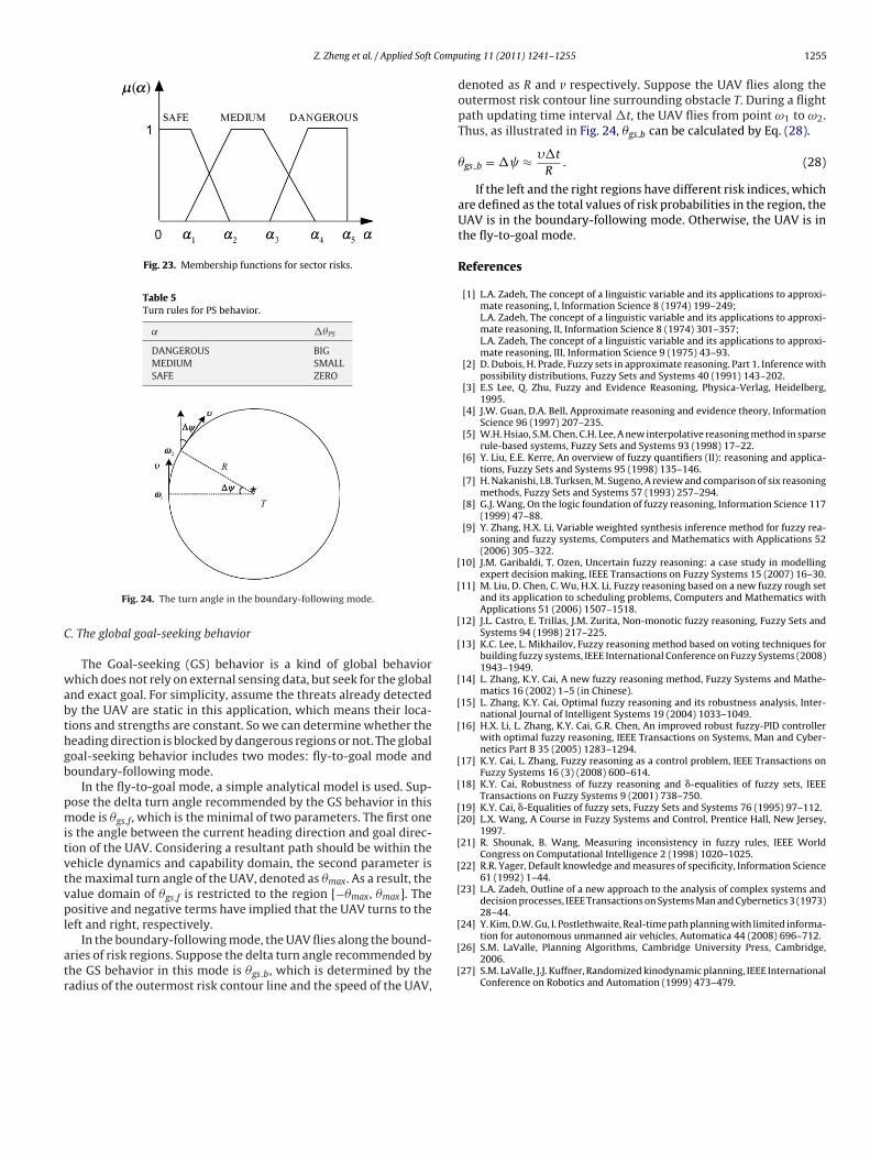
an example of the probabilistic risk distribution in [0, 200] × [0,200] (km) at a height of 2 (km) for 10 threats. The centre of eachcircle corresponds to the location of each threat, and the circlessurrounding the centers are risk contour lines. The outermost risklines correspond to Pi(w) = 0.08 in this example.

B. The regional path-searching behavior

The regional Path-Searching (PS) behavior navigates a UAV tothe safest (i.e. minimum risk) region in the located environment.Our algorithms do this by first inferring a Risk Index for each turndirection region based on the probabilistic risk in the region. Thenthe regional Risk Indices are used to develop the PS behavior’s fuzzyturn rules for detecting and avoiding dangerous region.

The motion control variable of the UAV is the turn angle. The turnangle is represented by three linguistic fuzzy sets {ZERO, SMALL,BIG}, with the membership functions shown in Fig. 22. The riskindex ˛ for one sector (Left, Front or Right as shown in Fig. 11) isdefined as the total values of risk probabilities in the region, andthen it is represented by three linguistic fuzzy sets {DANGEROUS,MEDIUM, SAFE}, with the membership functions shown in Fig. 23.

The UAV tends to fly toward the region that is safer. That is tosay, if the risk of the left sector is not smaller than that of the right,the UAV flies to the right region, and if the risk of the right sector islarger than that of the left, the UAV flies to the left region. The turnangles are inferred using the turn rules shown in Table 5. The rules

Fig. 22. Membership functions for turn angles.


Fig. 23. Membership functions for sector risks.

Table 5Turn rules for PS behavior.

˛ ��PS

DANGEROUS BIGMEDIUM SMALLSAFE ZERO

C

wabthgb

pmitvtvpl

atr

[

[

[

[

[

[

[

[

[

[[

[

[

[

Fig. 24. The turn angle in the boundary-following mode.

. The global goal-seeking behavior

The Goal-seeking (GS) behavior is a kind of global behaviorhich does not rely on external sensing data, but seek for the global

nd exact goal. For simplicity, assume the threats already detectedy the UAV are static in this application, which means their loca-ions and strengths are constant. So we can determine whether theeading direction is blocked by dangerous regions or not. The globaloal-seeking behavior includes two modes: fly-to-goal mode andoundary-following mode.

In the fly-to-goal mode, a simple analytical model is used. Sup-ose the delta turn angle recommended by the GS behavior in thisode is �gs f, which is the minimal of two parameters. The first one

s the angle between the current heading direction and goal direc-ion of the UAV. Considering a resultant path should be within theehicle dynamics and capability domain, the second parameter ishe maximal turn angle of the UAV, denoted as �max. As a result, thealue domain of �gs f is restricted to the region [−�max, �max]. Theositive and negative terms have implied that the UAV turns to the

eft and right, respectively.In the boundary-following mode, the UAV flies along the bound-

ries of risk regions. Suppose the delta turn angle recommended byhe GS behavior in this mode is �gs b, which is determined by theadius of the outermost risk contour line and the speed of the UAV,

[

[

[

uting 11 (2011) 1241–1255 1255

denoted as R and v respectively. Suppose the UAV flies along theoutermost risk contour line surrounding obstacle T. During a flightpath updating time interval�t, the UAV flies from point ω1 to ω2.Thus, as illustrated in Fig. 24, �gs b can be calculated by Eq. (28).

�gs b =� ≈ ��t

R. (28)

If the left and the right regions have different risk indices, whichare defined as the total values of risk probabilities in the region, theUAV is in the boundary-following mode. Otherwise, the UAV is inthe fly-to-goal mode.

References

[1] L.A. Zadeh, The concept of a linguistic variable and its applications to approxi-mate reasoning, I, Information Science 8 (1974) 199–249;L.A. Zadeh, The concept of a linguistic variable and its applications to approxi-mate reasoning, II, Information Science 8 (1974) 301–357;L.A. Zadeh, The concept of a linguistic variable and its applications to approxi-mate reasoning, III, Information Science 9 (1975) 43–93.

[2] D. Dubois, H. Prade, Fuzzy sets in approximate reasoning. Part 1. Inference withpossibility distributions, Fuzzy Sets and Systems 40 (1991) 143–202.

[3] E.S Lee, Q. Zhu, Fuzzy and Evidence Reasoning, Physica-Verlag, Heidelberg,1995.

[4] J.W. Guan, D.A. Bell, Approximate reasoning and evidence theory, InformationScience 96 (1997) 207–235.

[5] W.H. Hsiao, S.M. Chen, C.H. Lee, A new interpolative reasoning method in sparserule-based systems, Fuzzy Sets and Systems 93 (1998) 17–22.

[6] Y. Liu, E.E. Kerre, An overview of fuzzy quantifiers (II): reasoning and applica-tions, Fuzzy Sets and Systems 95 (1998) 135–146.

[7] H. Nakanishi, I.B. Turksen, M. Sugeno, A review and comparison of six reasoningmethods, Fuzzy Sets and Systems 57 (1993) 257–294.

[8] G.J. Wang, On the logic foundation of fuzzy reasoning, Information Science 117(1999) 47–88.

[9] Y. Zhang, H.X. Li, Variable weighted synthesis inference method for fuzzy rea-soning and fuzzy systems, Computers and Mathematics with Applications 52(2006) 305–322.

10] J.M. Garibaldi, T. Ozen, Uncertain fuzzy reasoning: a case study in modellingexpert decision making, IEEE Transactions on Fuzzy Systems 15 (2007) 16–30.

11] M. Liu, D. Chen, C. Wu, H.X. Li, Fuzzy reasoning based on a new fuzzy rough setand its application to scheduling problems, Computers and Mathematics withApplications 51 (2006) 1507–1518.

12] J.L. Castro, E. Trillas, J.M. Zurita, Non-monotic fuzzy reasoning, Fuzzy Sets andSystems 94 (1998) 217–225.

13] K.C. Lee, L. Mikhailov, Fuzzy reasoning method based on voting techniques forbuilding fuzzy systems, IEEE International Conference on Fuzzy Systems (2008)1943–1949.

14] L. Zhang, K.Y. Cai, A new fuzzy reasoning method, Fuzzy Systems and Mathe-matics 16 (2002) 1–5 (in Chinese).

15] L. Zhang, K.Y. Cai, Optimal fuzzy reasoning and its robustness analysis, Inter-national Journal of Intelligent Systems 19 (2004) 1033–1049.

16] H.X. Li, L. Zhang, K.Y. Cai, G.R. Chen, An improved robust fuzzy-PID controllerwith optimal fuzzy reasoning, IEEE Transactions on Systems, Man and Cyber-netics Part B 35 (2005) 1283–1294.

17] K.Y. Cai, L. Zhang, Fuzzy reasoning as a control problem, IEEE Transactions onFuzzy Systems 16 (3) (2008) 600–614.

18] K.Y. Cai, Robustness of fuzzy reasoning and �-equalities of fuzzy sets, IEEETransactions on Fuzzy Systems 9 (2001) 738–750.

19] K.Y. Cai, �-Equalities of fuzzy sets, Fuzzy Sets and Systems 76 (1995) 97–112.20] L.X. Wang, A Course in Fuzzy Systems and Control, Prentice Hall, New Jersey,

1997.21] R. Shounak, B. Wang, Measuring inconsistency in fuzzy rules, IEEE World

Congress on Computational Intelligence 2 (1998) 1020–1025.22] R.R. Yager, Default knowledge and measures of specificity, Information Science

61 (1992) 1–44.23] L.A. Zadeh, Outline of a new approach to the analysis of complex systems and

decision processes, IEEE Transactions on Systems Man and Cybernetics 3 (1973)28–44.

24] Y. Kim, D.W. Gu, I. Postlethwaite, Real-time path planning with limited informa-tion for autonomous unmanned air vehicles, Automatica 44 (2008) 696–712.

26] S.M. LaValle, Planning Algorithms, Cambridge University Press, Cambridge,2006.

27] S.M. LaValle, J.J. Kuffner, Randomized kinodynamic planning, IEEE InternationalConference on Robotics and Automation (1999) 473–479.

a feedback based cri approach to fuzzy reasoning

Documents