A Fault-tolerant Routing Strategy for Fibonacci-class Cubes

Zhang, Xinhua 1 and Peter, K K, Loh 2

1 Department of Computer Science, National University of Singapore, Singapore xinhua.zhang@nus.edu.sg

2 School of Computer Engineering, Nanyang Technological University, Singapore askkloh@ntu.edu.sg

Abstract. Fibonacci Cubes (FCs), together with the enhanced and extended forms, are a family of interconnection topologies formed by diluting links from binary hypercube. While they scale up more slowly, they provide more choices of network size. Despite sparser connectivity, they allow efficient emulation of many other topologies. However, there is no existing fault-tolerant routing strategy for FCs or other node/link diluted cubes. In this paper, we propose a unified fault-tolerant routing strategy for all Fibonacci-class Cubes, tolerating as many faulty components as network node availability. The algorithm is livelock free and generates deadlock-free routes, whose length is bounded linearly to network dimensionality. As a component, a generic approach to avoiding im-mediate cycles is designed which is applicable to a wide range of in-ter-connection networks, with computational and spatial complexity at O(1) and O(n log n) respectively. Finally, the performance of the algorithm is presented and analyzed through software simulation, showing its feasibility.

1 Introduction

Fibonacci-class Cubes originate from Fibonacci Cube (FC) proposed by Hsu [1], and its extended forms are Enhanced Fibonacci Cube (EFC) by Qian [2] and Extended Fibonacci Cube (XFC) by Wu [3]. This class of interconnection network uses fewer links than the corresponding binary hypercube, with the scale increasing at

(((1 3) 2) )nO + , slower than O(2n) for binary hypercube. This allows more choices of network size. In structural aspects, the two extensions virtually maintain all desirable properties of FC and improve it by ensuring the Hamiltonian property [2,3]. Besides, there is an ordered relationship of containment between the series of XFC and EFC, together with binary hypercube and regular FC. Lastly, they all allow efficient emula-tion of other topologies such as binary tree (including its variants) and binary hyper-cube. In essence, Fibonacci-class Cubes are superior to binary hypercube for low growth rate and sparse connectivity, with little loss of its desirable topological and functional (algorithmic) properties.

Though Fibonacci-class Cubes provide more options of incomplete hypercubes to which a faulty hypercube can be reconfigured and thus tend to find applications in fault-tolerant computing for degraded hypercubic computer systems, there are, to the

best of the authors’ knowledge, no existing fault-tolerant routing algorithms for them. This is also a common problem for link-diluted hypercubic variants. In this paper, we propose a unified fault-tolerant routing strategy for Fibonacci-class Cubes, named Fault-Tolerant Fibonacci Routing (FTFR), with following strengths: • It is applicable to all Fibonacci-class Cubes in a unified fashion, with only minimal

modification of structural representation. • The maximum number of faulty components tolerable is the network’s node avail-

ability [4] (the maximum number of faulty neighbors of a node that can be tolerated without disconnecting the node from the network).

• For a n-dimensional Fibonacci-class Cube, each node of degree deg maintains and updates at most (deg + 2) n⋅ bits’ vector information, among which: 1) a n-bit availability vector indicating the local non-faulty links, 2) a n-bit input link vector indicating the input message link, 3) all neighbors’ n-bit availability vector, indi-cating their link availability.

• Provided the number of component faults in the network does not exceed the net-work’s node availability, and the source and destination nodes are not faulty, FTFR guarantees that a message path length does not exceed n H+ empirically and 2n H+ theoretically, where n is the dimensionality of the network and H is the Hamming distance between source and destination.

• Generates deadlock-free and livelock-free routes. • Can be implemented almost entirely with simple and practical routing hardware

requiring minimal processor control. The rest of this paper is organized as follows. Section 2 reviews several versions of

definitions of Fibonacci-class Cube, together with initial analysis on their properties. Section 3 presents a Generic Approach to Cycle-free Routing (GACR), which is used as a component of the whole strategy. Section 4 elaborates on the algorithm FTFR. The design of a simulator and simulation results will be presented in section 5. Finally, the paper is concluded in section 6.

2 Preliminaries

2.1 Definitions

Though Fibonacci-class Cubes are very similar and are all based on a sequence with specific initial conditions, they do have some different properties that require special attention. The well-known Fibonacci number is defined by: 0 0,f =

1 1 21, n n nf f f f− −= = + for 2n ≥ . In [1], the order-n Fibonacci code of integer [0, 1] ( 3)ni f n∈ − ≥ is defined as 1 3 2( , , , )n Fb b b− ⋅ ⋅ ⋅ where bj is either 0 or 1 for

2 ( 1)j n≤ ≤ − and 12

nj j ji b f−== ∑ . Then Fibonacci Cube of order n ( 3n ≥ ) is a graph

( ), ( )n n nFC V f E f=< > , where ( ) {0, 1, , 1}n nV f f= ⋅⋅⋅ − and ( , ) ( )ni j E f∈ if and only if the Hamming distance between IF and JF is 1, where IF, JF stand for the Fibonacci codes of i and j, respectively. An equivalent definition is: let ( , )n n nFC V E= , then

3 {1, 0}V = , 4 {01, 00, 10}V = and 1 20 || 10 ||n n nV V V− −= ∪ for 5n ≥ , where || de-notes the concatenation operation and has higher precedence than union operation ∪ . Two nodes in nFC are connected by an edge in nE if and only if their Hamming distance is 1. To facilitate a unified discussion of Fibonacci-class Cubes, Vn can be a further defined in an obviously equivalent form: a set of all possible ( 2)n − -bit binary numbers, none of which has two consecutive 1’s. This definition is important for the discussion of properties in the next sub-section.

Enhanced Fibonacci Cube and Extended Fibonacci Cube can be defined in a similar way. Let ,n n nEFC V E= < > denote the Enhanced Fibonacci Cube of order n ( 3n ≥ ), then 3 {1,0}V = , 4 {01, 00, 10}V = , 5 {001, 101, 100, 000, 010}V = , 6 {0001,V = 0101, 0100, 0000, 0010, 1010, 1000, 1001} and 2 200 || 10 ||n n nV V V− −= ∪

4 40100 || 0101||n nV V− −∪ ∪ for 7n ≥ . Two nodes in EFCn are connected by an edge in

nE if and only if their labels differ in exactly one bit position, i.e., Hamming distance is 1.

A series of Extended Fibonacci Cubes is defined as { ( ) | 1,kXFC n k ≥ 2}n k≥ + , where ( ) { ( ), ( )}k k kXFC n V n E n= , ( ) 0 || ( 1) 10 || ( 2)k k kV n V n V n= − −∪ for 4n k≥ + . As initial conditions for recursion, ( 2) {0, 1}k

kV k + = meaning the Cartesian product of k sets of {0, 1}, and 1( 3) {0, 1}k

kV k ++ = . Two nodes in ( )kXFC n are connected by an edge in ( )kE n if and only if their Hamming distance is 1.

2.2 Properties of Fibonacci-class Cubes

In this section, we introduce an important property for our algorithm. Let current node address be u and destination node address be d, then each dimension corre-sponding to 1 in u d⊕ is called preferred dimension, where ⊕ stands for bitwise XOR operation. Other dimensions are called spare dimension. As Fibonacci-class Cubes are defined by link dilution, it is likely that links in some preferred dimensions are not available at a packet’s current node. But the following proposition guarantees that in a fault-free setting, there is always at least one preferred dimension available at the present node. Unlike in binary hypercube, this is not a trivial result.

(Proposition 1) In a fault-free FC, EFC or XFC, there is always a preferred dimension available at the packet’s present node before the destination is reached.

Proof : Consider an n-dimensional Fibonacci-class Cube, which means FC, XFC and EFC of order n + 2. Let the binary address of current node be 1 1 0na a a− ⋅ ⋅ ⋅ and the destination be 1 1 0nd d d− ⋅ ⋅ ⋅ . Let the rightmost (least significant) bit correspond to di-mension 0 while the leftmost bit correspond to dimension 1n − .

Case I: Fibonacci Cube FCn + 2. Obviously, if the destination has not been reached, there is always a preferred dimension [0, 1]i n∈ − . If 1ia = and 0id = , then there is always a preferred link available at dimension i because changing one ‘1’ in a valid address into 0 always produces a new valid address. So we only need to consider

0ia = and 1id = . When 3n ≤ , the proposition can be easily proven by enumeration. So now we suppose 4n ≥ .

1) If [1, 2]i n∈ − , then 1 0id − = , 1 0id + = . If 1 1ia − = , then i – 1 is an available pre-ferred dimension. If 1 1ia + = , then 1i + is an available preferred dimension. If

1 1 0i ia a− += = , then dimension i is an available preferred dimension because inverting

ia to 1 will not produce two consecutive 0’s in the new nodes address. 2) If i = 0, then d1= 0. If a1 = 1, dimension 1 is an available preferred dimension. If a1

= 0, then dimension 0 is an available preferred dimension because setting a0 to 1 will give a valid address.

3) If i = n – 1, then d n – 2 = 0. If an – 2 = 1, then dimension n – 2 is an available pre-ferred dimension. If 2 0na − = , then dimension 1n − is an available preferred dimen-sion.

Case II: XFCk (n+2). Suppose there is a preferred dimension i. If i k< , then in-verting ia will always produce a valid address. If i k≥ , the discussion is the same as case I.

Case III: EFCn+2. The discussion is similar to case I, but much more complicated. Basically, we just need to discuss over the leftmost preferred dimension. Detailed proof is omitted here due to limited space, but is available at http://www.comp.nus.edu.sg/~zhangxi2/proof.pdf. g

The proposition implies that whenever a spare dimension is used, either a faulty component is encountered or all neighbors on preferred dimensions have been visited previously. For the latter case, all such preferred dimensions must have been used as spare dimensions sometime before. So both cases can be boiled down to the encounter of faulty components (now or before). It is also implied that certain algorithm can be applied to all the three types of network and the existence of at least one preferred dimension is guaranteed in a certain sense, given the number of faulty components does not exceed node availability. This is the underlying idea of FTFR.

3 Generic Approach to Cycle-Free Routing (GACR)

As a component of FTFR, we digress from the mainframe for one section and pro-pose now a generic approach to avoiding cycles in routing by checking the traversal history. The algorithm takes only O(1) time to update the coded history record and O(n) time to check whether a neighbor has been visited before (can be virtually reduced to O(1) by utilizing parallelism). Other advantages include its wide applicability and easy hardware implementation. It applies to all networks in which links only connect node pairs whose Hamming distance is 1 (called Hamming link). All networks constructed by node or link dilution meet this criterion. An extended form of the algorithm can be applied to those networks with O(1) types of non-Hamming links at each node. Thus, such networks as Folded Hypercube, Enhanced Hypercube and Josephus Cube [5] can also use this algorithm.

3.1 Basic GACR

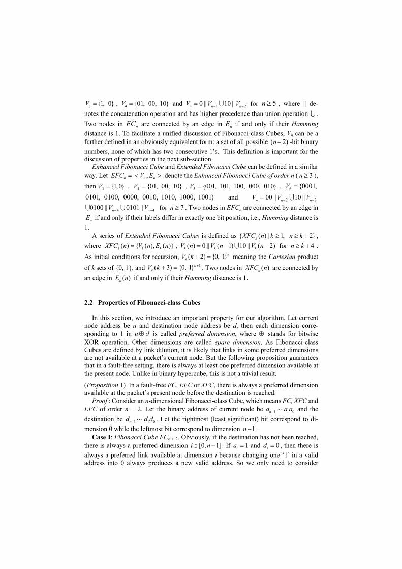
The traversal history is effectively an ordered sequence of dimensions used when leaving each visited node. We use Figure 1 for illustration.

Fig. 1. Basic GACR illustration

The route that originates from 000 can be recorded as: 1210121. An obvious equivalent condition for a route to contain a cycle is: there exists a way of inserting ‘(’ and ‘)’ into the sequence such that each number in the parenthesis appears for an even number of times. For example, in 1(21012), 0 appears only one time. In (1210121), 1 and 2 appear for an even time but 0 still appears for an odd number of times. So neither case forms a cycle. But for a sequence of 1234243, there must be a cycle: 1(234243). Suppose at node p, the history sequence is 1 2 na a a⋅ ⋅ ⋅ , and it is guaranteed that no cycle exists hitherto, then to check whether using dimension 1na + will cause any cycle, we only need to check whether in 1( )n na a + , 2 1 1( )n n n na a a a− − + , 4 3 2 1 1( )n n n n n na a a a a a− − − − + … each number will appear for an even number of time.

We first introduce the basic form of this algorithm that applies only to networks constructed by node/link dilution from binary hypercube. This algorithm is run at each intermediate node to ensure that the next node has never been visited before.

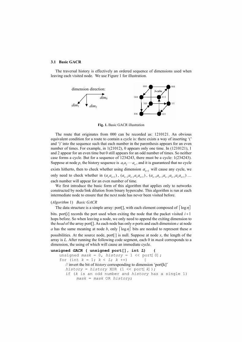
(Algorithm 1) Basic GACR The data structure is a simple array: port[], with each element composed of log n

bits. port[i] records the port used when exiting the node that the packet visited 1i + hops before. So when leaving a node, we only need to append the exiting dimension to the head of the array port[]. As each node has only n ports and each dimension c at node a has the same meaning at node b, only log n bits are needed to represent these n possibilities. At the source node, port[ ] is null. Suppose at node x, the length of the array is L. After running the following code segment, each 0 in mask corresponds to a dimension, the using of which will cause an immediate cycle. unsigned GACR ( unsigned port[], int L) {

unsigned mask = 0, history = 1 << port[0]; for (int k = 1; k < L; k ++) {

// invert the bit of history corresponding to dimension ‘port[k]’ history = history XOR (1 << port[k]); if (k is an odd number and history has a single 1)

mask = mask OR history;

dim0

dim1 dim2

dimension direction:

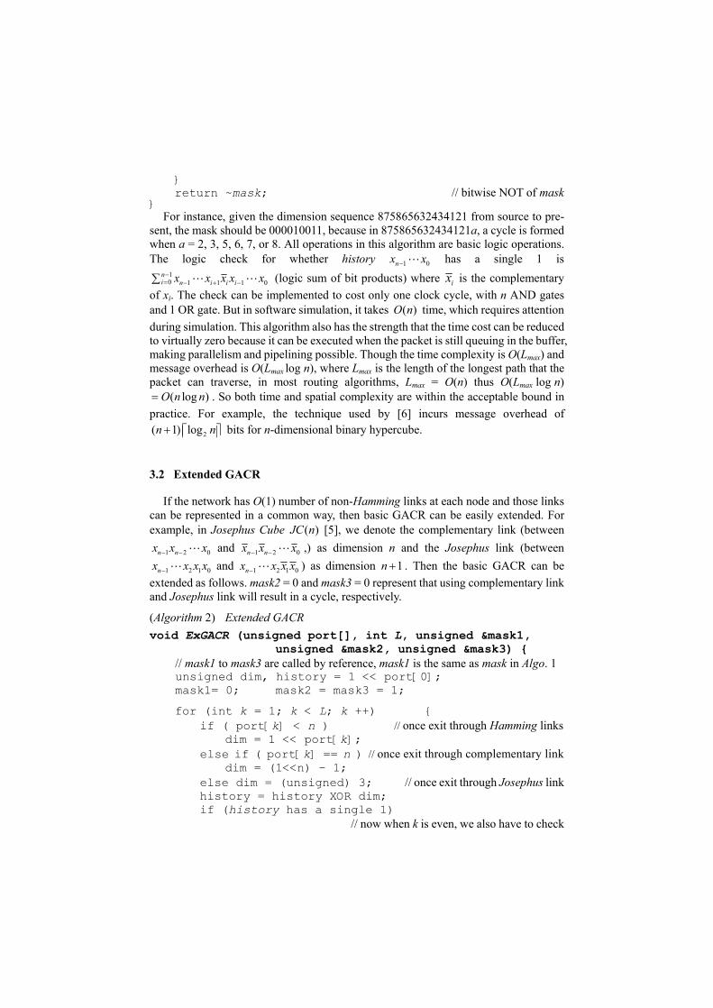
} return ~mask; // bitwise NOT of mask

} For instance, given the dimension sequence 875865632434121 from source to pre-

sent, the mask should be 000010011, because in 875865632434121a, a cycle is formed when a = 2, 3, 5, 6, 7, or 8. All operations in this algorithm are basic logic operations. The logic check for whether history 1 0nx x− L has a single 1 is

10 1 1 1 0

ni n i i ix x x x x−= − + −∑ L L (logic sum of bit products) where ix is the complementary

of xi. The check can be implemented to cost only one clock cycle, with n AND gates and 1 OR gate. But in software simulation, it takes ( )O n time, which requires attention during simulation. This algorithm also has the strength that the time cost can be reduced to virtually zero because it can be executed when the packet is still queuing in the buffer, making parallelism and pipelining possible. Though the time complexity is O(Lmax) and message overhead is O(Lmax log n), where Lmax is the length of the longest path that the packet can traverse, in most routing algorithms, Lmax = O(n) thus O(Lmax log n)

( log )O n n= . So both time and spatial complexity are within the acceptable bound in practice. For example, the technique used by [6] incurs message overhead of

2( 1) logn n+ bits for n-dimensional binary hypercube.

3.2 Extended GACR

If the network has O(1) number of non-Hamming links at each node and those links can be represented in a common way, then basic GACR can be easily extended. For example, in Josephus Cube ( )JC n [5], we denote the complementary link (between

1 2 0n nx x x− − L and 1 2 0n nx x x− − L ,) as dimension n and the Josephus link (between

1 2 1 0nx x x x− L and 1 2 1 0nx x x x− L ) as dimension 1n + . Then the basic GACR can be extended as follows. mask2 = 0 and mask3 = 0 represent that using complementary link and Josephus link will result in a cycle, respectively.

(Algorithm 2) Extended GACR void ExGACR (unsigned port[], int L, unsigned &mask1,

unsigned &mask2, unsigned &mask3) { // mask1 to mask3 are called by reference, mask1 is the same as mask in Algo. 1 unsigned dim, history = 1 << port[0]; mask1= 0; mask2 = mask3 = 1; for (int k = 1; k < L; k ++) {

if ( port[k] < n ) // once exit through Hamming links dim = 1 << port[k];

else if ( port[k] == n ) // once exit through complementary link dim = (1<<n) – 1; else dim = (unsigned) 3; // once exit through Josephus link history = history XOR dim;

if (history has a single 1) // now when k is even, we also have to check

mask1 = mask1 OR history; // for cycles caused by Hamming link else if (history is straight 1)

// check if history has straight 1’s for the cycle caused by complementary link mask2 = 0; else if (history = = (unsigned) 3)

// check the rightmost two bits for the cycles caused by Josephus link mask3 = 0; } mask1 = ~ mask1;

}

4 Fault-tolerant Fibonacci Routing (FTFR)

4.1 Definition and notation

Now we will go back to the mainframe of the routing strategy. In a Fibonacci-class Cube of order n + 2 (n-dimensional), each node’s address is a n-bit binary number. Let the source node s be (an–1 L a1a0) {0, 1}n∈ and the destination node d be (dn–1 L d1d0) {0, 1}n∈ . Denote the neighbor of node u along the i–

th dimension (0 )i n≤ < as ( )iu , by inverting the i th bit of u’s binary address. For convenience we define following terms.

1) input link vector I (x). An n-bit input link vector at node x is defined as I (x) = [ln–1 … l1 l0], where li = 0 if the message goes to the current node along the dimension i link ( 0 i n≤ < ). lj = 1 for j i≠ . Setting the corresponding bit to 0 for a used input link prevents the link from being used again immediately for message transmission, causing the message to “oscillate” back and forth. An input link vector has straight 1’s for a new message.

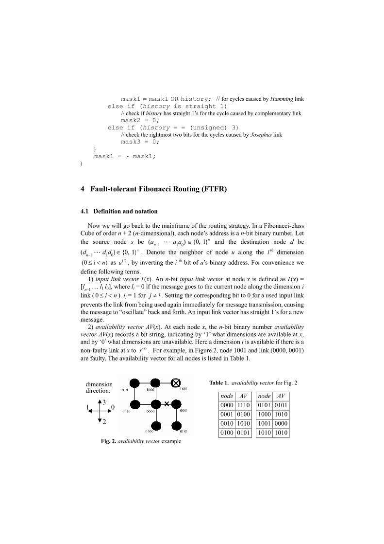
2) availability vector AV(x). At each node x, the n-bit binary number availability vector AV(x) records a bit string, indicating by ‘1’ what dimensions are available at x, and by ‘0’ what dimensions are unavailable. Here a dimension i is available if there is a non-faulty link at x to ( )ix . For example, in Figure 2, node 1001 and link (0000, 0001) are faulty. The availability vector for all nodes is listed in Table 1.

Table 1. availability vector for Fig. 2

node AV node AV 0000 1110 0101 0101 0001 0100 1000 1010 0010 1010 1001 0000 0100 0101 1010 1010

0

2

1 3

dimension direction:

Fig. 2. availability vector example

Availability vector is crucial for the generic applicability of the routing algorithm to all Fibonacci-class Cubes. It is in essence a distributed representation of network to-pology and fault distribution.

3) mask vector DT. To prevent cycles in the message path actively (not only by checking the immediate cycle at each step), a mask vector is introduced as part of the message overhead, defined as DT = 1 1 0[ ]nt t t− ⋅ ⋅ ⋅ . At source node, DT is cleared to be straight 1. After that, whenever a spare dimension is used, the corresponding bit in DT is set to 0 and cannot be set back to 1. Spare dimensions whose corresponding bit in DT is 0 cannot be used, i.e., dimensions that are spare at the source node can be used for at most two times. But different from many existing algorithms (e.g. [7]), each dimension which is preferred at the source can be used more than once. When it is used for the first time, DT doesn’t record it. But when it is used as a spare dimension later, the corre-sponding bit in DT is masked, so that it can’t be used as a spare dimension again. Fi-nally, each node periodically exchanges its own availability vector with all neighbors.

4.2 Description of FTFR

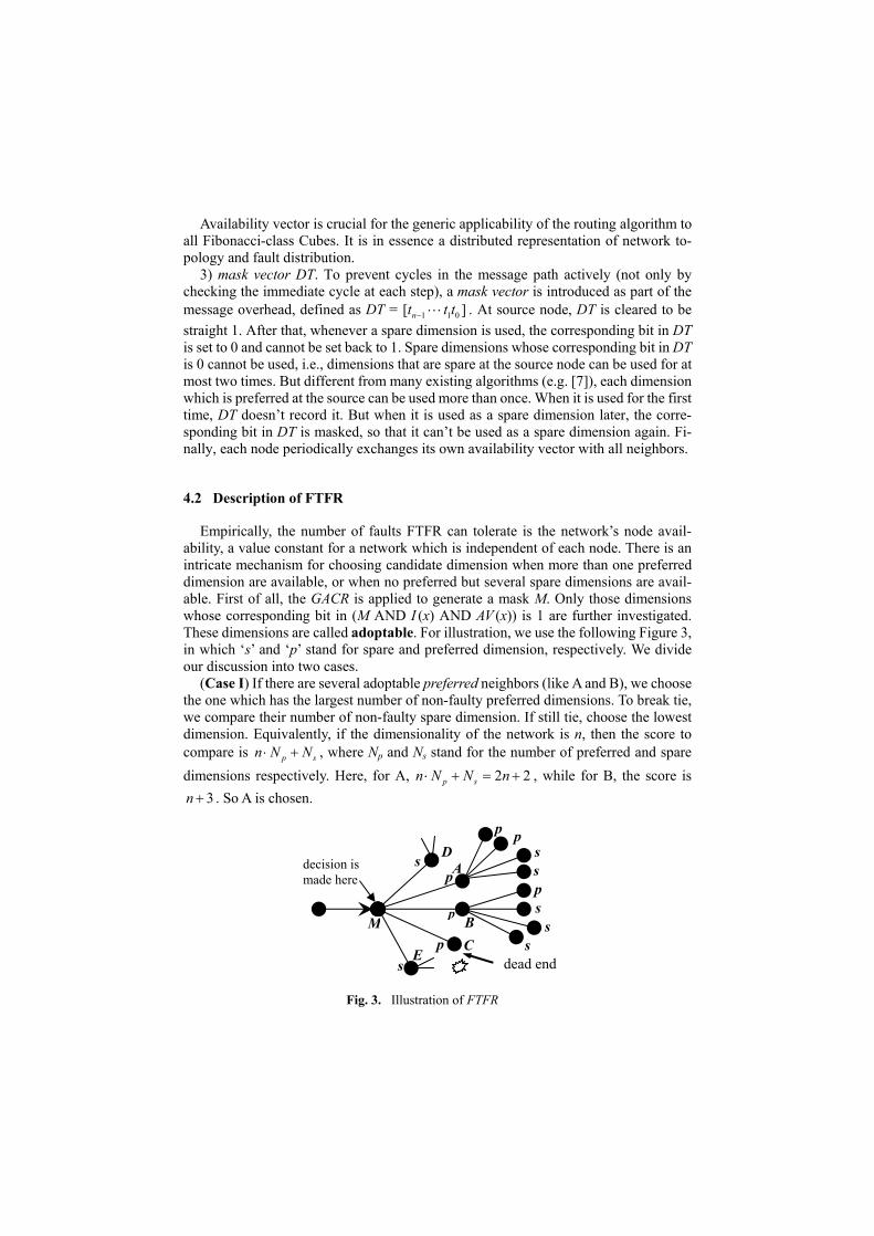
Empirically, the number of faults FTFR can tolerate is the network’s node avail-ability, a value constant for a network which is independent of each node. There is an intricate mechanism for choosing candidate dimension when more than one preferred dimension are available, or when no preferred but several spare dimensions are avail-able. First of all, the GACR is applied to generate a mask M. Only those dimensions whose corresponding bit in (M AND I (x) AND AV (x)) is 1 are further investigated. These dimensions are called adoptable. For illustration, we use the following Figure 3, in which ‘s’ and ‘p’ stand for spare and preferred dimension, respectively. We divide our discussion into two cases.

(Case I) If there are several adoptable preferred neighbors (like A and B), we choose the one which has the largest number of non-faulty preferred dimensions. To break tie, we compare their number of non-faulty spare dimension. If still tie, choose the lowest dimension. Equivalently, if the dimensionality of the network is n, then the score to compare is p sn N N⋅ + , where Np and Ns stand for the number of preferred and spare dimensions respectively. Here, for A, 2 2p sn N N n⋅ + = + , while for B, the score is

3n + . So A is chosen.

p

decision is made here

dead end

p s

B MC

D

E

Fig. 3. Illustration of FTFR

p

p s

A

p s

s p s

s s

(Case II) If at current node M, there are no adoptable preferred dimensions, spare dimensions have to be used, like D and E. Firstly, the eligibility is checked by DT. Then just like in case I, we compare n ⋅ Np + Ns. After one spare dimension is finally chosen, its corresponding bit in DT is masked to 0, so that it will not be used as spare dimension again.

The m = n ⋅ Np + Ns is a heuristic score. After extensive experiment, it is found that minor modifications can be made to m so as to improve the performance of FTFR. Suppose the dimension under consideration is i and inverting the ith bit of destination d produces d (i). If d (i) is a valid node address in that Fibonacci-class Cube, attaching some priority to dimension i will be helpful in reducing the number of hops. Hence, we add the value of network node availability to m for that candidate dimension in such a case.

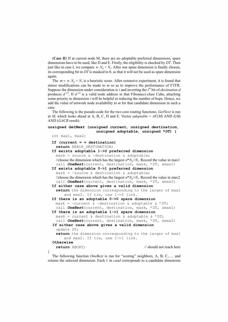
The following is the pseudo-code for the two core routing functions. GetNext is run at M, which looks ahead at A, B, C, D and E. Vector adoptable = AV(M) AND I(M) AND (GACR result).

unsigned GetNext (unsigned current, unsigned destination, unsigned adoptable, unsigned *DT) {

int max1, max2; If (current = = destination) return REACH_DESTINATION;

If exists adoptable 1->0 preferred dimension mask = source & ~destination & adoptable; //choose the dimension which has the largest n*Np+Ns. Record the value in max1 call OneBest(current, destination, mask, *DT, &max1)

If exists adoptable 0->1 preferred dimension mask = ~source & destination & adoptable;

//choose the dimension which has the largest n*Np+Ns. Record the value in max2 call OneBest(current, destination, mask, *DT, &max2)

If either case above gives a valid dimension return the dimension corresponding to the larger of max1

and max2. If tie, use 1->0 link. If there is an adoptable 0->0 spare dimension mask = ~current & ~destination & adoptable & *DT;

call OneBest(current, destination, mask, *DT, &max1) If there is an adoptable 1->1 spare dimension mask = current & destination & adoptable & *DT;

call OneBest(current, destination, mask, *DT, &max2) If either case above gives a valid dimension update DT;

return the dimension corresponding to the larger of max1 and max2. If tie, use 1->1 link.

Otherwise return ABORT; // should not reach here }

The following function OneBest is run for “scoring” neighbors, A, B, C,…. and returns the selected dimension. Each 1 in cand corresponds to a candidate dimension

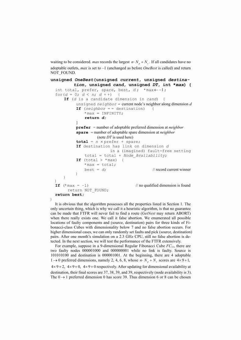
waiting to be considered. max records the largest p sn N N⋅ + . If all candidates have no adoptable outlets, max is set to –1 (unchanged as before OneBest is called) and return NOT_FOUND.

unsigned OneBest(unsigned current, unsigned destina-tion, unsigned cand, unsigned DT, int *max) {

int total, prefer, spare, best, d ; *max 1← − ; for(d = 0; d < n; d + +) { If (d is a candidate dimension in cand) {

unsigned neighbor = current node’s neighbor along dimension d If (neighbor = = destination) { *max = INFINITY; return d;

} prefer = number of adoptable preferred dimension at neighbor spare = number of adoptable spare dimension at neighbor

(note DT is used here) total = n × prefer + spare; If destination has link on dimension d

in a (imagined) fault-free setting total = total + Node_Availability; If (total > *max) { *max = total; best = d; // record current winner } } } If (*max = –1) // no qualified dimension is found return NOT_FOUND; return best;

} It is obvious that the algorithm possesses all the properties listed in Section 1. The

only uncertain thing, which is why we call it a heuristic algorithm, is that no guarantee can be made that FTFR will never fail to find a route (GetNext may return ABORT) when there really exists one. We call it false abortion. We enumerated all possible locations of faulty components and (source, destination) pairs for three kinds of Fi-bonacci-class Cubes with dimensionality below 7 and no false abortion occurs. For higher dimensional cases, we can only randomly set faults and pick (source, destination) pairs. After one month’s simulation on a 2.3 GHz CPU, still no false abortion is de-tected. In the next section, we will test the performance of the FTFR extensively.

For example, suppose in a 9-dimensional Regular Fibonacci Cube FC11, there are two faulty nodes 000001000 and 000000001 while no link is faulty. Source is 101010100 and destination is 000001001. At the beginning, there are 4 adoptable 1 → 0 preferred dimensions, namely 2, 4, 6, 8, whose p sn N N⋅ + scores are 4 9 1,× + 4 9 2, 4 9 0, 4 9 0× + × + × + respectively. After updating for dimensional availability at destination, their final scores are 37, 38, 39, and 39, respectively (node availability is 3). The 0 → 1 preferred dimension 0 has score 39. Thus dimension 6 or 8 can be chosen

and we use the smaller one. After using dimension 6 8 0 4 0 2, the packet reaches 000000000, where neither of the two preferred dimensions (3 and 0) is adoptable be-cause they both lead to a faulty node. So a spare dimension has to be used. The input dimension is 2 and using dimension 4 will lead to cycle. Therefore, there are only 5 adoptable dimensions, namely 1, 5, 6, 7, 8. Their scores are: 14, 25, 25, 25, and 27, respectively. So spare dimension 8 is chosen and its corresponding bit in DT is masked.

5 Simulation Results

A software simulator is constructed to imitate the behavior of the real network [8, 9], and thus test the performance of our algorithm. The assumptions are: (1) fixed packet-sized messages, (2) source and destination nodes must be non-faulty, (3) eager readership is employed when packet service rate is faster than packet arrival rate, (4) a node is faulty when all of its incident links are faulty, (5) a node knows status of its links to its neighboring nodes, (6) all faults are fail-stop, (7) location of faults, source and destination are all randomly chosen by uniform distribution.

The performance of the routing algorithms is measured by two metrics: average latency and throughput. Average latency is defined as LP/DP, where LP is the total latency of all packets that have reached destination while DP is the number of those packets. Throughput is defined as DP/PT, where PT is the total routing process time taken by all nodes.

5.1 Comparison of FTFR’s Performance on Various Network Sizes

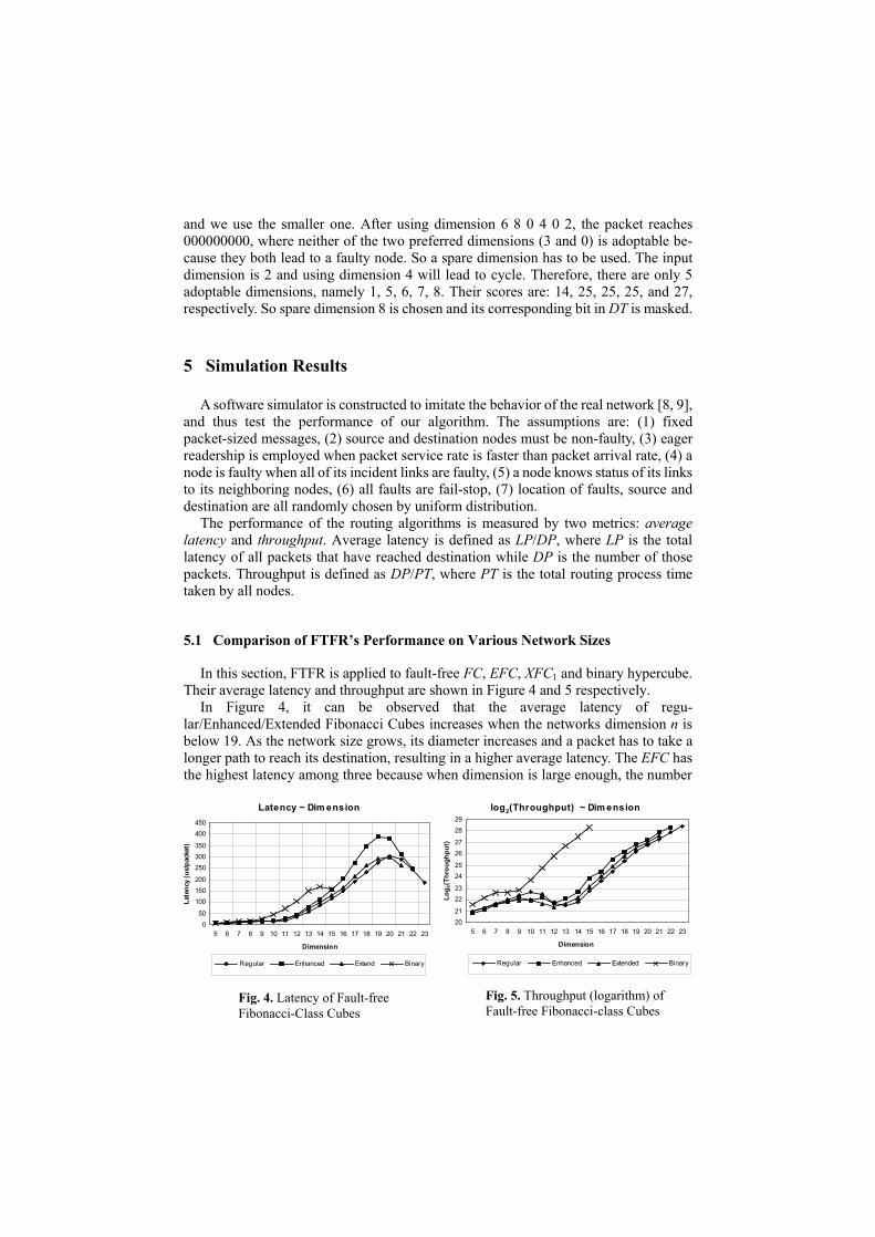
In this section, FTFR is applied to fault-free FC, EFC, XFC1 and binary hypercube. Their average latency and throughput are shown in Figure 4 and 5 respectively.

In Figure 4, it can be observed that the average latency of regu-lar/Enhanced/Extended Fibonacci Cubes increases when the networks dimension n is below 19. As the network size grows, its diameter increases and a packet has to take a longer path to reach its destination, resulting in a higher average latency. The EFC has the highest latency among three because when dimension is large enough, the number

log2(Throughput) ~ Dim ension

2021

2223

2425

2627

2829

5 6 7 8 9 10 11 12 13 14 15 16 17 18 19 20 21 22 23

Dimension

Log 2

(Thr

ough

put)

Regular Enhanced Extended Binary

Latency ~ Dim ension

050

100150200

250300350

400450

5 6 7 8 9 10 11 12 13 14 15 16 17 18 19 20 21 22 23

Dimension

Late

ncy

(us/

pack

et)

Regular Enhanced Extend Binary

Fig. 4. Latency of Fault-free Fibonacci-Class Cubes

Fig. 5. Throughput (logarithm) of Fault-free Fibonacci-class Cubes

of nodes in EFC is the largest among Fibonacci-class Cubes of the same dimension. After the dimension reaches 19 or 20, the latency decreases. This is because the scale of the network becomes so large that the simulation time is insufficient to saturate the network with packets, i.e., the number of packets reaching destination is lower than the total allowable packet number. So the packets in these networks spend less time waiting in output queue or injection queue, while that portion of time comprises a major part of latency for lower dimensional networks that get saturated with packets during the simulation. As n = 19~20 is already adequate for demonstrating the performance of FTFR, we do not wait for network saturation. Binary hypercube, a special type of XFC, shows a similar trend, with latency starting to decrease at n = 15. This also goes well with the fact that the number of nodes in Fibonacci-class Cube and binary hypercube are ((1 3) / 2 )n nO + and O(2n) respectively. (1 3) / 2 : 2+ ≈ 15:20. Due to limited physical memory, simulation for binary hypercube is conducted up to n = 15.

In Figure 5, it is demonstrated that the throughput of all networks is increasing as the dimension increases from 12 to over 20. This is due to the parallelism of the networks and the increase in the number of nodes, which can generate and route packets in the network, is faster as compared with the FTFR time complexity O(n log n). By in-creasing the network size, the number of links is also increasing at a higher rate than the node number. This in turn increases the total allowable packets in the network. With parallelism, more packets will be delivered in a given duration. For the same reason mentioned in the previous discussion of latency, EFC has the largest throughput among the three types of Fibonacci-class Cube. An interesting observation is that for dimen-sions between 11~13, the throughput decreases and increases again afterwards. One possible explanation is: the complexity of FTFR is O(n log n). For large n, the variation in log n is small compared with small n. Thus the difference given by log n will be small and the trend of throughput is similar to an O(n) routing algorithm. For small n, how-ever, the contribution of log n is comparable with the increase rate of networks size, which leads to the seemingly irregularity. On the other hand, when dimension is small (below 11), the network is too small to display this characteristic. For Fibonacci-class Cube, the irregular interval is 11~13, while for binary hypercube, such an interval is 8~9. This again tallies with (1 3) / 2+ : 2 ≈ 8.5:12.

5.2 Comparison of FTFR’s Performance on Various Numbers of Faults

In this sub-section, the performance of FTFR is measured by the varying the number of faulty components in network. The result for XFC13(16) is shown in Figure 6.

It is clear that when the number of faults increases, the trend of average latency is to increase while the throughput is to decrease. This is because when more faults appear, the packet is more likely to use spare dimensions which make the final route longer. In consequence, the latency increases and throughput decreases. However, there are some special situations when the existence of faults reduces the number of alternative output ports available, and thus accelerates the routing process. The varying number of faults has more evident influence when the network size is small. With fixed number of faults, there are fewer paths available for routing in smaller networks than in larger ones. Thus

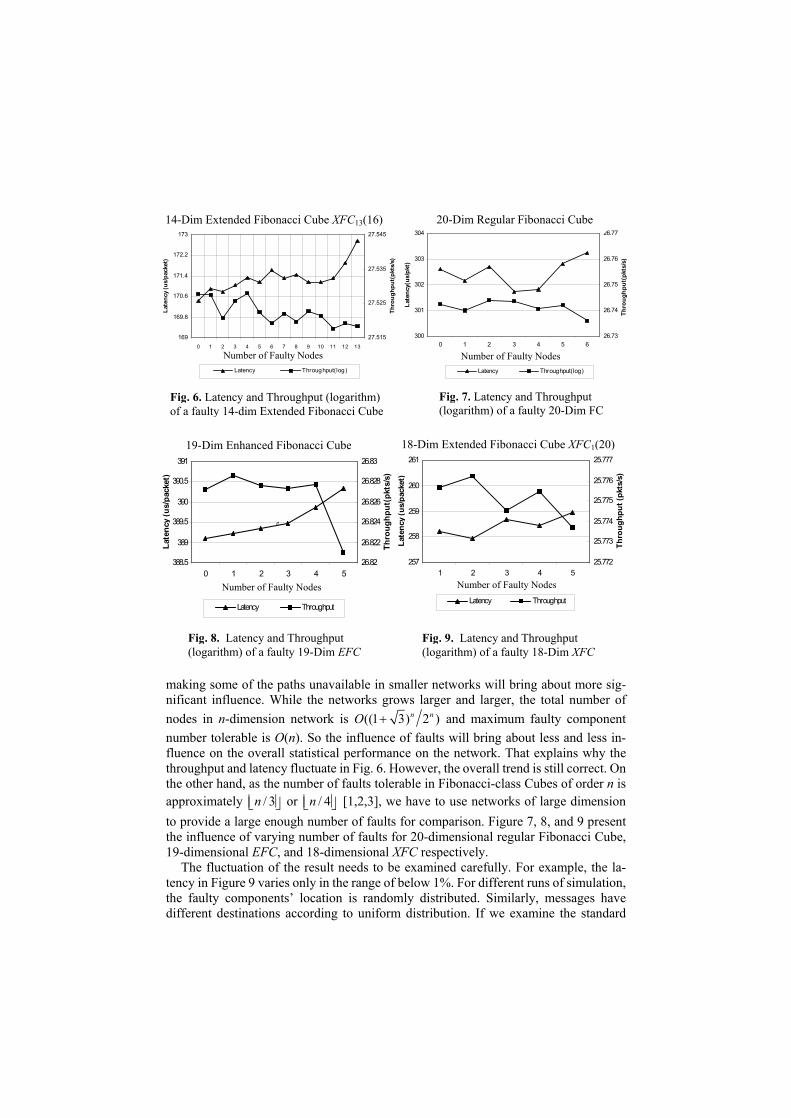
making some of the paths unavailable in smaller networks will bring about more sig-nificant influence. While the networks grows larger and larger, the total number of nodes in n-dimension network is ((1 3) 2 )n nO + and maximum faulty component number tolerable is O(n). So the influence of faults will bring about less and less in-fluence on the overall statistical performance on the network. That explains why the throughput and latency fluctuate in Fig. 6. However, the overall trend is still correct. On the other hand, as the number of faults tolerable in Fibonacci-class Cubes of order n is approximately / 3n or / 4n [1,2,3], we have to use networks of large dimension to provide a large enough number of faults for comparison. Figure 7, 8, and 9 present the influence of varying number of faults for 20-dimensional regular Fibonacci Cube, 19-dimensional EFC, and 18-dimensional XFC respectively.

The fluctuation of the result needs to be examined carefully. For example, the la-tency in Figure 9 varies only in the range of below 1%. For different runs of simulation, the faulty components’ location is randomly distributed. Similarly, messages have different destinations according to uniform distribution. If we examine the standard

14-Dim Extended Fibonacci Cube XFC13(16)

169

169.8

170.6

171.4

172.2

173

0 1 2 3 4 5 6 7 8 9 10 11 12 13

Number of Faulty Nodes

Late

ncy

(us/

pack

et)

27.515

27.525

27.535

27.545

Thro

ughp

ut(p

kts/

s)

Latency Throughput(log )

Fig. 6. Latency and Throughput (logarithm) of a faulty 14-dim Extended Fibonacci Cube

20-Dim Regular Fibonacci Cube

300

301

302

303

304

0 1 2 3 4 5 6Number of Faulty Nodes

Late

ncy(

us/p

kt)

26.73

26.74

26.75

26.76

26.77

Thro

ughp

ut(p

kts/

s)

Latency Throughput(log)

Fig. 7. Latency and Throughput (logarithm) of a faulty 20-Dim FC

Fig. 8. Latency and Throughput (logarithm) of a faulty 19-Dim EFC

Fig. 9. Latency and Throughput (logarithm) of a faulty 18-Dim XFC

19-Dim Enhanced Fibonacci Cube

388.5

389

389.5

390

390.5

391

0 1 2 3 4 5Number of Faulty Nodes

Late

ncy

(us/

pack

et)

26.82

26.822

26.824

26.826

26.828

26.83

Thro

ughp

ut(p

kts/

s)

Latency Throughput

d

18-Dim Extended Fibonacci Cube XFC1(20)

257

258

259

260

261

1 2 3 4 5Number of Faulty Nodes

Late

ncy

(us/

pack

et)

25.772

25.773

25.774

25.775

25.776

25.777

Thro

ughp

ut (p

kts/

s)

Latency ThroughputNumber of Faulty Nodes Number of Faulty Nodes

Number of Faulty Nodes Number of Faulty Nodes

19-Dim Enhanced Fibonacci Cube 18-Dim Extended Fibonacci Cube XFC1(20)

20-Dim Regular Fibonacci Cube 14-Dim Extended Fibonacci Cube XFC13(16)

deviation of the result (not shown), it is observed that such a small variation as in Figure 9 is within the 95% confidence interval for almost all situations. Thus, it is more rea-sonable to focus on the trend of the statistical results, rather than the exact value.

6 Conclusion

In this paper, a new effective fault-tolerant routing strategy is proposed for Fibo-nacci-class Cubes in a unified fashion. It is livelock free and generates deadlock-free routes with the path length strictly bounded. The space and computation complexity as well as message overhead size are all moderate. Although the Fibonacci-class Cubes may be very sparsely connected, the algorithm can tolerate as many faulty components as the network node availability. The component mechanism which ensures cy-cle-freeness is also generically applicable to a wide range of network topologies. Simulation results show that the algorithm scales well with network size and is em-pirically immune to false abortion. Future work needs to be done on further increasing the number of faulty components tolerable, possibly by careful categorization of faults based on their specific location as in [8]. Physical implementation, such as Field Pro-grammable Gate Array, can also be done to evaluate the algorithm’s efficiency and feasibility more accurately.

References

1. Hsu, W. J. (1993). Fibonacci Cubes-A New Interconnection Topology. IEEE Transactions on Parallel and Distributed Systems 4[1], 3-12.

2. Qian, H. & Hsu, W. J. (1996). Enhanced Fibonacci Cubes. The Computer Journal 39[4], 331-345.

3. Wu, J. (1997). Extended Fibonacci Cubes. IEEE Transactions on Parallel and Distributed Systems 8[12], 1203-1210.

4. Fu, A. W. & Chau, S. (1998). Cyclic-Cubes: A New Family of Interconnection Networks of Even Fixed-Degrees. IEEE Transactions on Parallel and Distributed Systems 9[12], 1253-1268.

5. Loh, P. K. K. & Hsu, W. J. (1999). The Josephus Cube: A Novel Interconnection Network. Journal of Parallel Computing 26, 427-453.

6. Chen, M.-S. & Shin, K. G. (1990). Depth-First Search Approach for Fault-Tolerant Routing in Hypercube Multicomputers. IEEE Transactions on Parallel and Distributed Systems 1[2], 152-159.

7. Lan, Y. (1995). An Adaptive Fault-Tolerant Routing Algorithm for Hypercube Multicom-puters. IEEE Transactions on Parallel and Distributed Systems 6[11], 1147-1152.

8. Loh, P. K. K. & Zhang, X. (2003). A fault-tolerant routing strategy for Gaussian cube using Gaussian tree. 2003 International Conference on Parallel Processing Workshops, 305-312.

9. Zhang, Xinhua (2003). Analysis of Fuzzy-Nero Network Communications. Undergraduate Final Year Project, Nanyang Technological University.