A fast tabu search algorithm for the group shop scheduling problem

S.Q. Liu, H.L. Ong*, K.M. Ng

Department of Industrial and Systems Engineering, National University of Singapore, 10 Kent Ridge Crescent, Singapore 119260, Singapore

Received 3 June 2004; received in revised form 19 November 2004; accepted 2 February 2005

Available online 16 March 2005

Abstract

Three types of shop scheduling problems, the flow shop, the job shop and the open shop scheduling problems, have been widely studied in

the literature. However, very few articles address the group shop scheduling problem introduced in 1997, which is a general formulation that

covers the three above mentioned shop scheduling problems and the mixed shop scheduling problem. In this paper, we apply tabu search to

the group shop scheduling problem and evaluate the performance of the algorithm on a set of benchmark problems. The computational results

show that our tabu search algorithm is typically more efficient and faster than the other methods proposed in the literature. Furthermore, the

proposed tabu search method has found some new best solutions of the benchmark instances.

q 2005 Elsevier Ltd. All rights reserved.

Keywords: Machine scheduling; Flow shop; Open shop; Job shop; Mixed shop; Group shop

1. Introduction

The machine scheduling problems can be classified into

two types according to the characteristics of the relationship

between the jobs and operations: the single-stage production

systems and the multi-stage production systems. In a single-

stage production system, each job consists of only one

operation, whereas in multi-stage production systems, each

job generally consists of more than one operation, each of

which requiring a different machine to process at a time.

There are three main types of multi-stage production

systems, namely the flow shop scheduling (FSS) problem,

the job shop scheduling (JSS) problem, and the open shop

scheduling (OSS) problem. In a flow shop, the operations of

each job have to be processed on machines in the same

order. In a job shop, which is a generalization of the flow

shop, the operations of each job have to be processed in a

given order on the machines, but different jobs may have

different orders. In an open shop, the processing order of the

operations for each job is unrestricted. These three shop

scheduling problems have been studied for a long time since

the 1950s. They are known to be NP-hard and hence difficult

0965-9978/$ - see front matter q 2005 Elsevier Ltd. All rights reserved.

doi:10.1016/j.advengsoft.2005.02.002

* Corresponding author. Tel.: C65 6874 2562; fax: C65 6777 1434.

E-mail address: iseonghl@nus.edu.sg (H.L. Ong).

to solve optimally [1,2]. The difficulty of the problem may

be illustrated by the fact that the optimal solution of a

10-machine 10-job JSS instance, formulated by Fisher and

Thompson in 1963 [3], was not found until more than

20 years after the problem was introduced. In fact, this

instance was exactly solved for the first time in 1989 by

Carlier and Pinson with a branch and bound algorithm

which requires 5 h of computing time on PRIME 2655 [4].

Furthermore, although several methods were proposed to

deal with the permutation FSS problem, a special case of the

general FSS problem, very few papers address the general

FSS problem [5]. Most research activities aimed at tackling

the OSS problem have long been dominated by exact

approaches, such as branch and bound methods. The first

state-of-the-art metaheuristic for the OSS problem was

developed by Liaw in 1999 [6].

In 1985, the term mixed shop scheduling (MSS) problem

for describing a more general type of a multi-stage

production system was introduced by Masuda et al. [7]. In

MSS, the machine routes of jobs can either be fixed or

unrestricted. The MSS problem can also be regarded as a

mixture of the above three shop scheduling problems. In

1997, the group shop scheduling (GSS) problem was first

introduced in the context of a mathematical competition

organized by the TU Eindhoven, Netherlands [8].

Similar to the MSS problem, the GSS problem contains

the characteristics of the FSS, JSS, and OSS problems. As a

result, the methodology for solving the MSS problem can

Advances in Engineering Software 36 (2005) 533–539

www.elsevier.com/locate/advengsoft

0 1 2

3 4 5 6

7 8 9

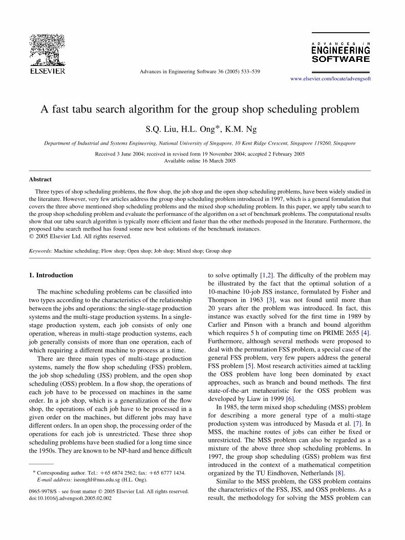
Fig. 1. The graph for one GSS instance.

S.Q. Liu et al. / Advances in Engineering Software 36 (2005) 533–539534

also be applied to the GSS problem with some modification.

To our knowledge, very few articles in the literature address

the application of metaheuristics to the MSS and GSS

problems [9,10].

Actually, one may consider the class of shop scheduling

problems discussed above as arising from two possible

sources. One is the static shop scheduling problems, such as

jobs to be processed in a production department where

machine requirement and task order are assumed to be

known. Consequently, it is reasonable to assume that the

problem falls into a specified category of shop scheduling

problems discussed above. The other possible source

consists of jobs that are dynamic in nature. For instance,

the jobs to be processed in a maintenance workshop may

arrive dynamically. In this situation, the job characteristics

and requirements change with time and consequently, the

user does not have full control over them. This type of

scheduling problems which are more interesting but difficult

to solve, have been referred to as a protean system or

dynamic shop scheduling problems in the literature [11,12].

In this paper, we focus on the static job shop scheduling

problems and extend the neighborhood structure and the

tabu search method of Liu and Ong [5,10] for solving the

FSS, JSS, OSS and MSS problems to the GSS problem.

The rest of this paper is organized as follows. Section 2

describes the GSS problem. Section 3 presents three

neighborhood structures used by the tabu search for the

GSS problem. Section 4 outlines the tabu search algorithm

implemented in this study. The computational results for a

number of benchmark instances are presented in Section 5.

Finally, some concluding remarks are given in Section 6.

0 4 7

1 3 8

2 6

5 9

F L

Job 1 Job 2 Job 3

Machine 1

Machine 2

Machine 3

Machine 4

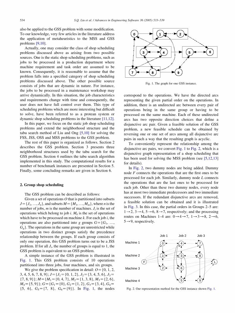
Fig. 2. Our representation method for the GSS instance shown Fig. 1.

2. Group shop scheduling

The GSS problem can be described as follows:

Given a set of operations O that is partitioned into subsets

JZ{J1, ., Jn}, and subsets MZ{M1, ., Mm}, where n is the

number of jobs, m is the number of machines. Ji is the set of

operations which belong to job i. Mk is the set of operations

which have to be processed on machine k. For each job i, the

operations are also partitioned into g groups GZ{G1, .,

Gg}. The operations in the same group are unrestricted while

operations in two distinct groups satisfy the precedence

relationship between the groups. If each group consists of

only one operation, this GSS problem turns out to be a JSS

problem. If for all Ji, the number of groups is equal to 1, the

GSS problem is equivalent to an OSS problem.

A simple instance of the GSS problem is illustrated in

Fig. 1. This GSS problem consists of 10 operations

partitioned into three jobs, four machines, and six groups.

We give the problem specification in detail: OZ{0, 1, 2,

3, 4, 5, 6, 7, 8, 9}; JZ{J1Z{0, 1, 2}, J2Z{3, 4, 5, 6}, J3Z{7, 8, 9}}; MZ{M1Z{0, 4, 7}, M2Z{1, 3, 8}, M3Z{2, 6},

M4Z{5, 9}}; GZ{G1Z{0}, G2Z{1, 2}, G3Z{3, 4}, G4Z{5, 6}, G5Z{7, 8}, G6Z{9}}. In Fig. 1, the nodes

correspond to the operations. We have the directed arcs

representing the given partial order on the operations. In

addition, there is an undirected arc between every pair of

operations being in the same group or having to be

processed on the same machine. Each of these undirected

arcs has two opposite direction choices that define a

disjunctive arc pair. Given a feasible solution of the GSS

problem, a new feasible schedule can be obtained by

reversing one or one set of arcs among all disjunctive arc

pairs in such a way that the resulting graph is acyclic.

To conveniently represent the relationship among the

disjunctive arc pairs, we convert Fig. 1 to Fig. 2, which is a

disjunctive graph representation of a shop scheduling that

has been used for solving the MSS problem (see [5,12,13]

for details).

In Fig. 2, two dummy nodes are being added. Dummy

node F connects the operations that are the first ones to be

processed for each job. Similarly, dummy node L connects

the operations that are the last ones to be processed for

each job. Other than these two dummy nodes, every node

has at most two immediate predecessors and two immediate

successors. If the redundant disjunctive arcs are removed,

a feasible solution can be obtained and it is illustrated

in Fig. 3. In this case, the partial orders in Groups 2–5 are:

1/2, 3/4, 5/6, 8/7, respectively; and the processing

routes on Machines 1–4 are: 0/4/7, 1/3/8, 2/6,

5/9, respectively.

0 4 7

1 3 8

2 6

5 9

F L

Job 1 Job 2 Job 3

Machine 1

Machine 2

Machine 3

Machine 4

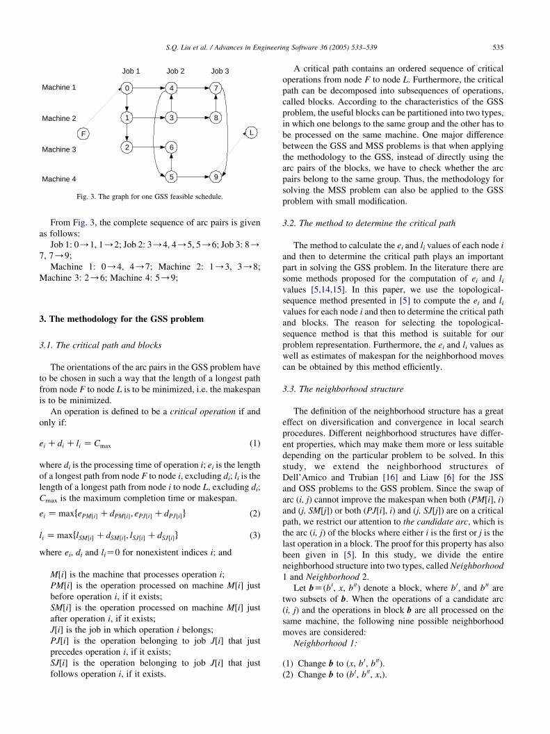
Fig. 3. The graph for one GSS feasible schedule.

S.Q. Liu et al. / Advances in Engineering Software 36 (2005) 533–539 535

From Fig. 3, the complete sequence of arc pairs is given

as follows:

Job 1: 0/1, 1/2; Job 2: 3/4, 4/5, 5/6; Job 3: 8/7, 7/9;

Machine 1: 0/4, 4/7; Machine 2: 1/3, 3/8;

Machine 3: 2/6; Machine 4: 5/9;

3. The methodology for the GSS problem

3.1. The critical path and blocks

The orientations of the arc pairs in the GSS problem have

to be chosen in such a way that the length of a longest path

from node F to node L is to be minimized, i.e. the makespan

is to be minimized.

An operation is defined to be a critical operation if and

only if:

ei Cdi C li Z Cmax (1)

where di is the processing time of operation i; ei is the length

of a longest path from node F to node i, excluding di; li is the

length of a longest path from node i to node L, excluding di;

Cmax is the maximum completion time or makespan.

ei Z maxfePM½i� CdPM½i�; ePJ½i� CdPJ½i�g (2)

li Z maxflSM½i� CdSM½i�; lSJ½i� CdSJ½i�g (3)

where ei, di and liZ0 for nonexistent indices i; and

M[i] is the machine that processes operation i;

PM[i] is the operation processed on machine M[i] just

before operation i, if it exists;

SM[i] is the operation processed on machine M[i] just

after operation i, if it exists;

J[i] is the job in which operation i belongs;

PJ[i] is the operation belonging to job J[i] that just

precedes operation i, if it exists;

SJ[i] is the operation belonging to job J[i] that just

follows operation i, if it exists.

A critical path contains an ordered sequence of critical

operations from node F to node L. Furthermore, the critical

path can be decomposed into subsequences of operations,

called blocks. According to the characteristics of the GSS

problem, the useful blocks can be partitioned into two types,

in which one belongs to the same group and the other has to

be processed on the same machine. One major difference

between the GSS and MSS problems is that when applying

the methodology to the GSS, instead of directly using the

arc pairs of the blocks, we have to check whether the arc

pairs belong to the same group. Thus, the methodology for

solving the MSS problem can also be applied to the GSS

problem with small modification.

3.2. The method to determine the critical path

The method to calculate the ei and li values of each node i

and then to determine the critical path plays an important

part in solving the GSS problem. In the literature there are

some methods proposed for the computation of ei and livalues [5,14,15]. In this paper, we use the topological-

sequence method presented in [5] to compute the ei and livalues for each node i and then to determine the critical path

and blocks. The reason for selecting the topological-

sequence method is that this method is suitable for our

problem representation. Furthermore, the ei and li values as

well as estimates of makespan for the neighborhood moves

can be obtained by this method efficiently.

3.3. The neighborhood structure

The definition of the neighborhood structure has a great

effect on diversification and convergence in local search

procedures. Different neighborhood structures have differ-

ent properties, which may make them more or less suitable

depending on the particular problem to be solved. In this

study, we extend the neighborhood structures of

Dell’Amico and Trubian [16] and Liaw [6] for the JSS

and OSS problems to the GSS problem. Since the swap of

arc (i, j) cannot improve the makespan when both (PM[i], i)

and (j, SM[j]) or both (PJ[i], i) and (j, SJ[j]) are on a critical

path, we restrict our attention to the candidate arc, which is

the arc (i, j) of the blocks where either i is the first or j is the

last operation in a block. The proof for this property has also

been given in [5]. In this study, we divide the entire

neighborhood structure into two types, called Neighborhood

1 and Neighborhood 2.

Let bZ(b 0, x, b 00) denote a block, where b 0, and b 00 are

two subsets of b. When the operations of a candidate arc

(i, j) and the operations in block b are all processed on the

same machine, the following nine possible neighborhood

moves are considered:

Neighborhood 1:

(1)

Change b to (x, b 0, b 00).

(2)

Change b to (b 0, b 00, x,).

S.Q. Liu et al. / Advances in Engineering Software 36 (2005) 533–539536

(3)

Change the set of arcs (PM[i], i, j) to (j, PM[i], i) if

PM[i] exists.

(4)

Change the set of arcs (PM[i], i, j) to (j, i, PM[i]) if

PM[i] exists.

(5)

Change the set of arcs (i, j, SM[j]) to (j, SM[j], i) if SM[j]

exists.

(6)

Change the set of arcs (i, j, SM[j]) to (SM[j], j, i) if SM[j]

exists.

(7)

Reverse arcs (i, j) and (PJ[j], j) at the same time if PJ[j]

and j are in the same group.

(8)

Reverse arcs (i, j) and (i, SJ[i]) at the same time if i and

SJ[i] are in the same group.

(9)

Reverse arcs (i, j), (PJ[j], j) and (i, SJ[i]) at the same

time if PJ[j] and j, i and SJ[i] are in the same group at

the same time.

When the operations of the candidate arc (i, j) and the

operations of block b are all in the same group, the following

nine possible neighborhood moves are considered:

Neighborhood 2:

(1)

Change b to (x, b 0, b 00).

(2)

Change b to (b 0, b 00, x,).

(3)

Change the set of arcs (PJ[i], i, j) to (j, PJ[i], i) if PJ[i]

exists.

(4)

Change the set of arcs (PJ[i], i, j) to (j, i, PJ[i]) if PJ[i]

exists.

(5)

Change the set of arcs (i, j, SJ[j]) to (j, SJ[j], i) if SJ[j]

exists.

(6)

Change the set of arcs (i, j, SJ[j]) to (SJ[j], j, i) if SJ[j]

exists.

(7)

Reverse arcs (i, j) and (PM[j], j) at the same time if

PM[j] exists.

(8)

Reverse arcs (i, j) and (i, SM[i]) at the same time if

SM[i] exists.

(9)

Reverse arcs (i, j), (PM[j], j) and (i, SM[i]) at the same

time if PM[j] and SM[i] exist at the same time.

For example, a possible neighborhood move for Case 1

of Neighborhood 1 is as follows:

PM[i]/i/j/SM[j]0j/PM[i]/i/SM[j]

The new ei and li values of the changed parameters can be

calculated as follows:

e0j Z maxfePM½PM½i�� CdPM½PM½i��; ePJ½j� CdPJ½j�g

e0PM½i� Z maxfePJ½PM½i�� CdPJ½PM½i��; e0j Cdjg

e0i Z maxfePJ½i� CdPJ½i�; e0PM½i� CdPM½i�g

l0i Z maxflSJ½i� CdSJ½i�; lSM½j� CdSM½j�g

l0PM½i� Z maxflSJ½PM½i�� CdSJ½PM½i��; l0i Cdig

l0j Z maxflSJ½j� CdSJ½j�; l0PM½i� CdPM½i�g

Z Z maxfe0j Cdj C l0j; e0PM½i� CdPM½i� C l0PM½i�; e

0i Cdi C l0ig

The value Z gives an estimate for the new makespan,

which is the length of the new longest path that passes

through at least one of nodes in the set {i, j, PM[i]}. In this

case, a directed cycle can occur if and only if there is a

directed path from SJ[PM[i]] to PJ[j], a directed path from

SJ[i] to PJ[j], or a directed path from SJ[i] to PJ[PM[i]] in

the new schedule. Therefore, this move is allowable only if

the following inequalities are satisfied:

ePJ½j� CdPJ½j�%eSJ½PM½i�� if PJ½j� and SJ½PM½i�� exist;

ePJ½j� CdPJ½j�%eSJ½i� if PJ½j� and SJ½i� exist;

ePJ½PM½i�� CdPJ½PM½i��%eSJ½i� if SJ½i� and PJ½PM½i�� exist:

4. The tabu search algorithm

The tabu search (TS) algorithm was initially proposed by

Glover in 1986 [17]. The basic ideas were also sketched by

Hansen in 1986 [18]. Additional formalizations for TS were

reported by Glover in 1989 and 1990 [19,20]. To our

knowledge, the first application of the TS algorithm to the

JSS problem was proposed by Taillard in 1994 [15]. Many

computational experiments have shown that TS has now

become an established approximation technique, which can

compete with almost all other known approaches.

The TS algorithm is an iterative improvement approach

designed to avoid terminating prematurely at a local

optimum for combinatorial optimization problems. Similar

to the simulating annealing (SA) and threshold accepting

(TA) algorithms, TS is based on the idea of exploring the

solution space of a problem by moving from one region of

search space to another in order to look for a better solution.

When a solution is stuck at a local optimum, SA or TA

attempts to escape from it by accepting an inferior solution,

which may lead to better solutions later. In contrast, TS

allows the search to move to the best solution among a set of

candidate moves as defined by the neighborhood structure.

However, subsequent iterations may cause the search to

move repeatedly back to the same local optimum. In order to

avoid cycling, moves that would bring back to a recently

visited solution should be forbidden or declared tabu for a

certain number of iterations. This is accomplished by

keeping the attributes of the forbidden moves in a list, called

tabu list.

The systematic use of memory is an essential feature of

tabu search. In this study, two types of tabu list are used as

the fundamental memory structure in TS to prevent cycling.

The first type of tabu list memorizes the complete job routes

on one machine as an element of this tabu list. In the

same fashion, the second type of tabu list keeps track of

the machine routes, that is, the assignment of machines for a

job. A move is admissible if the changed job route in

S.Q. Liu et al. / Advances in Engineering Software 36 (2005) 533–539 537

the new schedule does not have exactly the same order as

any element of the first type of tabu list, or the changed

machine route in the new schedule does not have exactly the

same order as any element of the second type of tabu list.

The definition of the tabu elements is the most important

feature for this TS algorithm.

Additionally, an aspiration criterion is defined to deal

with the case in which a move leading to a new best solution

is tabu. If a current tabu move satisfies the aspiration

criterion, its tabu status is canceled and it becomes an

allowable move. The use of the aspiration criterion allows

TS to lift the restrictions and intensify the search into a

particular solution region.

Furthermore, our computational experience reveals that

by using a large size of neighborhood space and tabu lists in

the TS algorithm, it would allow the search procedure to

find a solution which is close to the optimum faster, but this

could also cause the TS procedure to be stuck prematurely

after a certain number of iterations. To overcome this

drawback, we apply two methods to diversify the search

procedure: one is that we make randomized choices to

diminish the sizes of tabu lists and neighborhood space; the

other is that we incorporate the SA algorithm into the TS

algorithm and use the SA function to generate a new random

schedule. This strategy improves the performance of our TS

algorithm greatly. We deem this as a very important feature

of our TS algorithm which allows the algorithm to generate

very good solutions to the GSS problem.

5. Computational experiments

From the literature, there is only one real GSS instance,

whizzkids97 that is proposed for a mathematics competition

in 1997 at the TU Eindhoven, Netherlands [8]. However, all

other types of shop scheduling problems are special cases of

the GSS problem and so we can generate GSS instances

from the JSS benchmark instances.

To evaluate the performance of the TS algorithm

proposed in this study, we apply the algorithm to several

established benchmark instances taken from the literature.

These include the GSS benchmark instance generated from

the JSS problem instance ft10 (10 machines and 10 jobs,

[3]), la38 (15 machines and 15 jobs, [21]), and abz7

(15 machines and 20 jobs, [22]) by introducing groups of

various lengths into the jobs. All these GSS problem

instances used for testing the algorithms can be downloaded

from the website in [23]. The three sets of GSS instances

derived from ft10, la38, and abz7 are denoted by ft10_g,

la38_g, and abz7_g, respectively, where g is the group

length. For example, the GSS instance generated from ft10

with group length of 4 is denoted by ft10_4.

Our TS algorithm is coded in Visual CCC6.0 under

Microsoft Windows XP operating systems, running on a

Dell laptop with Intel Pentium IV 1.8 GHz processor and

256 Mb RAM. The results of the algorithm applied to 41

GSS instances are given in Table 1. The first column of

Table 1 indicates the problem instances. When the group

length is 1, these GSS instances (i.e. ft10_1, la38_1, and

abz7_1) are the original JSS instances. As the group length

increases, the instances are getting closer to the OSS

instances. When the group length is equal to m, these GSS

instances (i.e. ft10_10, la38_15, and abz7_15) become the

original OSS instances. In the second column of Table 1, the

best makespan values known in the literature are presented

for these benchmark GSS instances. The best solution found

in 20 runs, the average solution, the coefficient of variation

(defined to be the ratio of standard deviation/average!100),

and the average computation time are given in columns 3–6

of Table 1, respectively.

To provide a comparison of our TS algorithm against two

other methods, the ACO_GSS algorithm and the TS_GSS

algorithm recently proposed by Blum and Sampels [9], we

also show in Table 1 the results of these methods when

applied to the same instances. For ease of comparison, if the

solution found by our TS algorithm is better than the other

two methods, it is highlighted in bold.

In our TS algorithm, we do not set any limit on the

program running time. Since heuristics cannot be guaran-

teed to solve the GSS problem optimally, the best solution

found is compared with the well-known lower bound (LB)

value calculated by Eq. (4) [15]:

LB Z max maxj

Xn

iZ1

pij

( );max

i

Xm

jZ1

pij

( )( )(4)

The TS algorithm terminates when a solution is equal to

the LB value or the known optimal solution has been found,

or the number of iterations has reached a pre-specified

maximum iteration number.

The computational results are summarized as follows:

(a)

Our proposed TS algorithm can obtain very good

solutions for most of the GSS benchmark instances. By

comparing the results obtained by the other two

approaches, our TS algorithm outperforms them in the

sense that it can achieve better performance based on

three measures: the best solution found, the coefficient

of variation, and the average computation time. It is

noted that the computational times for the other two

algorithms reported in [9] were based on a 1.1 GHz

AMD Athlon CPU, which is different from our 1.8 GHz

Pentium IV CPU and hence difficult to compare.

However, after factoring the different CPU speeds (i.e.

computation time/processor speed), our TS is still faster

in general. The solution to most of the problem

instances tested can be obtained in less than 5 min of

CPU time. Our algorithm is more robust in the sense

that it has the smallest coefficient of variation amongst

the three algorithms tabulated in Table 1. In particular,

our TS has found new best solutions in 9 instances out

of these 41 instances, i.e. ft10_2, ft10_3, ft10_4,

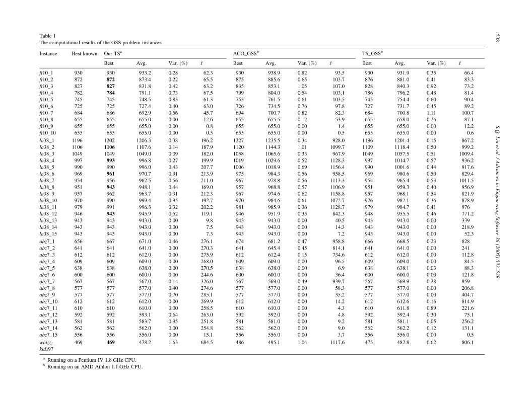
Table 1

The computational results of the GSS problem instances

Instance Best known Our TSa ACO_GSSb TS_GSSb

Best Avg. Var. (%) �t Best Avg. Var. (%) �t Best Avg. Var. (%) �t

ft10_1 930 930 933.2 0.28 62.3 930 938.9 0.82 93.5 930 931.9 0.35 66.4

ft10_2 872 872 873.4 0.22 65.5 875 885.6 0.65 103.7 876 881.0 0.41 83.3

ft10_3 827 827 831.8 0.42 63.2 835 853.1 1.05 107.0 828 840.3 0.92 73.2

ft10_4 782 784 791.1 0.73 67.5 799 804.0 0.54 103.1 786 796.2 0.48 81.4

ft10_5 745 745 748.5 0.85 61.3 753 761.5 0.61 103.5 745 754.4 0.60 90.4

ft10_6 725 725 727.4 0.40 63.0 726 734.5 0.76 97.8 727 731.7 0.45 89.2

ft10_7 684 686 692.9 0.56 45.7 694 700.7 0.82 82.3 684 700.8 1.11 100.7

ft10_8 655 655 655.0 0.00 12.6 655 655.5 0.12 53.9 655 658.0 0.26 87.1

ft10_9 655 655 655.0 0.00 0.8 655 655.0 0.00 1.4 655 655.0 0.00 12.2

ft10_10 655 655 655.0 0.00 0.5 655 655.0 0.00 0.5 655 655.0 0.00 0.6

la38_1 1196 1202 1206.3 0.38 196.2 1227 1235.5 0.34 928.0 1196 1201.4 0.15 867.2

la38_2 1106 1106 1107.6 0.14 187.9 1120 1144.3 1.01 1099.7 1109 1118.4 0.50 999.2

la38_3 1049 1049 1049.0 0.09 182.0 1058 1065.6 0.33 967.9 1049 1057.5 0.51 1009.4

la38_4 997 993 996.8 0.27 199.9 1019 1029.6 0.52 1128.3 997 1014.7 0.57 936.2

la38_5 990 990 996.0 0.43 207.7 1006 1018.9 0.69 1156.4 990 1001.6 0.44 917.6

la38_6 969 961 970.7 0.91 213.9 975 984.3 0.56 958.5 969 980.6 0.50 829.4

la38_7 954 956 962.5 0.56 211.0 967 978.8 0.56 1113.3 954 965.4 0.53 1011.5

la38_8 951 943 948.1 0.44 169.0 957 968.8 0.57 1106.9 951 959.3 0.40 956.9

la38_9 957 962 963.7 0.31 212.3 967 974.6 0.62 1158.8 957 968.1 0.54 821.9

la38_10 970 990 999.4 0.95 192.7 970 984.6 0.61 1072.7 976 982.1 0.36 878.9

la38_11 979 991 996.3 0.32 202.2 981 985.9 0.36 1128.7 979 984.7 0.41 976

la38_12 946 943 945.9 0.52 119.1 946 951.9 0.35 842.3 948 955.5 0.46 771.2

la38_13 943 943 943.0 0.00 9.8 943 943.0 0.00 40.5 943 943.0 0.00 339

la38_14 943 943 943.0 0.00 7.5 943 943.0 0.00 14.3 943 943.0 0.00 218.9

la38_15 943 943 943.0 0.00 7.3 943 943.0 0.00 7.2 943 943.0 0.00 52.3

abz7_1 656 667 671.0 0.46 276.1 674 681.2 0.47 958.8 666 668.5 0.23 828

abz7_2 641 641 641.0 0.00 270.3 641 645.4 0.45 814.1 641 641.0 0.00 241

abz7_3 612 612 612.0 0.00 275.9 612 612.4 0.15 734.6 612 612.0 0.00 112.8

abz7_4 609 609 609.0 0.00 268.0 609 609.0 0.00 96.5 609 609.0 0.00 84.5

abz7_5 638 638 638.0 0.00 270.5 638 638.0 0.00 6.9 638 638.1 0.03 88.3

abz7_6 600 600 600.0 0.00 244.6 600 600.0 0.00 36.4 600 600.0 0.00 121.8

abz7_7 567 567 567.0 0.14 326.0 567 569.0 0.49 939.7 567 569.9 0.28 959

abz7_8 577 577 577.0 0.40 274.6 577 577.0 0.00 58.3 577 577.0 0.00 206.8

abz7_9 577 577 577.0 0.70 285.1 577 577.0 0.00 35.2 577 577.0 0.00 404.7

abz7_10 612 612 612.0 0.00 269.9 612 612.0 0.00 14.2 612 612.6 0.16 814.9

abz7_11 610 610 610.0 0.00 258.5 610 610.0 0.00 4.3 610 611.8 0.89 221.6

abz7_12 592 592 593.1 0.64 263.0 592 592.0 0.00 4.8 592 592.4 0.30 75.1

abz7_13 581 581 583.7 0.95 251.8 581 581.0 0.00 9.2 581 581.1 0.05 256.2

abz7_14 562 562 562.0 0.00 254.8 562 562.0 0.00 9.0 562 562.2 0.12 131.1

abz7_15 556 556 556.0 0.00 15.1 556 556.0 0.00 3.7 556 556.0 0.00 0.5

whizz-

kids97

469 469 478.2 1.63 684.5 486 495.1 1.04 1117.6 475 482.8 0.62 806.1

a Running on a Pentium IV 1.8 GHz CPU.b Running on an AMD Athlon 1.1 GHz CPU.

S.Q

.L

iuet

al.

/A

dva

nces

inE

ng

ineerin

gS

oftw

are

36

(20

05

)5

33

–5

39

53

8

S.Q. Liu et al. / Advances in Engineering Software 36 (2005) 533–539 539

LA38_2, LA38_4, LA38_6, LA38_8, LA38_12, Whizz-

kids97, as highlighted in bold in Table 1.

(b)

To avoid premature convergence, the use of diversifica-

tion mechanism, such as making probabilistic choices

for diminishing the sizes of the tabu list and neighbor-

hood space as well as incorporating the SA function into

the TS algorithm to generate a new random schedule

when the search procedure is stuck prematurely or after

a given number of iterations, has greatly improved the

performance of the algorithm. For example, in the

Whizzkid97 instance, our TS algorithm is able to get

the makespan value of 496 from the initial makespan of

3684 in about 40 s (or about 5000 iterations). However,

it is very difficult to achieve the optimal value of 469 if

the time to diversify the search procedure is not

sufficiently long.

(c)

It is our aim to develop a methodology which can work

well on all types of shop scheduling problems,

especially for the MSS and GSS problems introduced

recently. The computational experiments for the GSS

problem show that the proposed methodology are not

only efficient but also very robust, because it can also be

applied to the MSS, OSS, JSS, and FSS problems

successfully [10].

6. Conclusion

In this paper, we apply tabu search to the group shop

scheduling problem and evaluate the performance of the

algorithm on a set of benchmark problems. The compu-

tational results show that our tabu search algorithm is

typically more efficient and faster than the other methods

proposed in the literature. Furthermore, the proposed tabu

search method has found some new best solutions of the

benchmark instances.

The representation method for the GSS problem, the

approach to compute the ei and li values and then determine

the critical path, the neighborhood structure, and the

implementation of the TS algorithm are four significant

parts in solving the GSS problem. The different represen-

tation methods of the schedule provide many possible

avenues to define the neighborhood structure and

implementation of algorithms. The approach to compute

the makespan or the ei and li values has a great effect on the

computation time of the entire search procedure. A powerful

neighborhood structure would provide a good search

direction to find the optimum solution faster. The TS

algorithm seems to direct the local search to move away

from local minima and explore the feasible region in its

entirety effectively with the use of diversification

mechanism.

It has been demonstrated that the proposed TS method-

ology is an efficient method for solving the GSS problem.

A further extension to this study is to apply the TS

methodology to other types of scheduling problems such as

the GSS problem in a dynamic scheduling environment and

the GSS problem in which the job information is partially

known.

Acknowledgements

The authors would like to thank the referees for their

constructive comments and suggestions that contributed to

the improvement of this paper.

References

[1] Garey MR, Johnson DS, Sethi R. The complexity of flowshop and

jobshop scheduling. Math Oper Res 1976;1:117–29.

[2] Lenstra JK, Rinnooy Kan AHG, Brucker P. Complexity of machine

scheduling problems. Ann Discrete Math 1977;1:343–62.

[3] Fisher H, Thompson GL. Probabilistic learning combinations of local

job-shop scheduling rules. Industrial scheduling. Englewood Cliffs,

NJ: Prentice Hall; 1963 p. 225–51.

[4] Carlier J, Pinson E. An algorithm for solving the job shop problem.

Manage Sci 1989;35:164–76.

[5] Liu SQ, Ong HL. A comparative study of algorithms for the flowshop

scheduling problem. Asia-Pacific J Oper Res 2002;19(2):205–22.

[6] Liaw CF. A tabu search algorithm for the open shop scheduling

problem. Comput Oper Res 1999;26:109–26.

[7] Masuda T, Ishii H, Nishida T. The mixed shop scheduling problem.

Discrete Appl Math 1985;11:175–86.

[8] http://www.win.tue.nl/whizzkids/1997, 1997.

[9] Blum C, Sampels M. An ant colony optimization algorithm for shop

scheduling problems. J Math Modell Algorithms 2004;3:285–308.

[10] Liu SQ, Ong HL. Metaheuristics for the mixed shop scheduling

problem. Asia-Pacific J Oper Res 2004;21(1):97–115.

[11] Kumar S. In: Masanori F, Kaoru T, editors. Optimization of protean

systems: a review, APORS 94, Fukuoka, Japan. World Scientific

Publishers; 1995. p. 139–46.

[12] Liu SQ, Ong HL, Ng KM. Metaheuristics for minimizing the

makespan of the dynamic shop scheduling problem. Adv Eng

Software 2005; 36:199–205.

[13] Roy B, Sussmann B. Les problems d’ordonnancement avec contra-

intes. Technique Report 9, SEMA. Note D.S. Paris; 1964.

[14] Bellman RE. On a routing problem. Q Appl Math 1958;16:87–90.

[15] Taillard E. Parallel taboo search techniques for the job shop

scheduling problem. ORSA J Comput 1994;6(2):108–17.

[16] Dell’Amico M, Trubian M. Applying tabu search to the job shop

scheduling problem. Ann Oper Res 1993;41:231–52.

[17] Glover F. Future paths for integer programming and links to artificial

intelligence. Comput Oper Res 1986;13:533–49.

[18] Hansen P. The steepest ascent mildest descent heuristic for

combinatorial programming. Talk presented at the Congress on

Numerical Methods in Combinatorial Optimization 1986, Capri.

[19] Glover F. Tabu search-part I. ORSA J Comput 1989;1(3):190–206.

[20] Glover F. Tabu search-part II. ORSA J Comput 1990;2(1):4–32.

[21] Lawrence S. Resource constrained project scheduling: an experimen-

tal investigation of heuristic scheduling techniques (supplement).

Technical report, Graduate School of Industrial Administration.

Pittsburgh: Carnegie Mellon University; 1984.

[22] Adams J, Balas E, Zawack D. The shifting bottleneck procedure for

job shop scheduling. Manage Sci 1988;34(3):391–401.

[23] http://www.lsi.upc.es/~cblum/.