a eﬃcient similarity joins for near duplicate detectionweiw/files/tods-ppjoin-final.pdf · a...

A

Efficient Similarity Joins for Near Duplicate Detection

Chuan Xiao, The University of New South Wales

Wei Wang, The University of New South Wales

Xuemin Lin, The University of New South Wales & East China Normal University

Jeffrey Xu Yu, Chinese University of Hong Kong

Guoren Wang, Northeastern University, China

With the increasing amount of data and the need to integrate data from multiple data sources, one ofthe challenging issues is to identify near duplicate records efficiently. In this paper, we focus on efficientalgorithms to find pair of records such that their similarities are no less than a given threshold. Severalexisting algorithms rely on the prefix filtering principle to avoid computing similarity values for all possiblepairs of records. We propose new filtering techniques by exploiting the token ordering information; theyare integrated into the existing methods and drastically reduce the candidate sizes and hence improve theefficiency. We have also studied the implementation of our proposed algorithm in stand-alone and RDBMS-based settings. Experimental results show our proposed algorithms can outperforms previous algorithms onseveral real datasets.

Categories and Subject Descriptors: H.3.3 [Information Search and Retrieval]: Search Process, Clus-tering

General Terms: Algorithm, Performance

Additional Key Words and Phrases: similarity join, near duplicate detection

ACM Reference Format:

Xiao, C., Wang, W., Lin, X., Yu, J. X., Wang, G. 2011. Efficient Similarity Joins for Near DuplicateDetection. ACM Trans. Datab. Syst. V, N, Article A (January YYYY), 40 pages.DOI = 10.1145/0000000.0000000 http://doi.acm.org/10.1145/0000000.0000000

1. INTRODUCTION

Near duplicate data is one of the issues accompanying the rapid growth of data on theInternet and the growing need to integrating data from heterogeneous sources. As a concreteexample, a sizeable percentage of the Web pages are found to be near-duplicates by severalstudies [Broder et al. 1997; Fetterly et al. 2003; Henzinger 2006]. These studies suggest thataround 1.7% to 7% of the Web pages visited by crawlers are near duplicate pages. Nearduplicate data bear high similarity to each other, yet they are not bitwise identical. Thereare many causes for the existence of near duplicate data: typographical errors, versioned,mirrored, or plagiarized documents, multiple representations of the same physical object,spam emails generated from the same template, etc.Identifying all the near duplicate objects benefits many applications. For example,

Wei Wang was partially supported by ARC DP0987273 and DP0881779. Xuemin Lin was partially supportedby ARC DP110102937, DP0987557, DP0881035, NSFC61021004, and Google Research Award.Author’s addresses: C. Xiao, W. Wang and X. Lin, School of Computer Science and Engineering, TheUniversity of New South Wales, Australia; J. X. Yu, Department of Systems Engineering and EngineeringManagement, Chinese University of Hong Kong, Hong Kong; G. Wang, Faculty of Information Science andTechnology, Northeastern University, China.Permission to make digital or hard copies of part or all of this work for personal or classroom use isgranted without fee provided that copies are not made or distributed for profit or commercial advantageand that copies show this notice on the first page or initial screen of a display along with the full citation.Copyrights for components of this work owned by others than ACM must be honored. Abstracting withcredit is permitted. To copy otherwise, to republish, to post on servers, to redistribute to lists, or to use anycomponent of this work in other works requires prior specific permission and/or a fee. Permissions may berequested from Publications Dept., ACM, Inc., 2 Penn Plaza, Suite 701, New York, NY 10121-0701 USA,fax +1 (212) 869-0481, or [email protected]© YYYY ACM 0362-5915/YYYY/01-ARTA $10.00DOI 10.1145/0000000.0000000 http://doi.acm.org/10.1145/0000000.0000000

ACM Transactions on Database Systems, Vol. V, No. N, Article A, Publication date: January YYYY.

A:2

— For Web search engines, identifying near duplicate Web pages helps to perform focusedcrawling, increase the quality and diversity of query results, and identify spams [Fetterlyet al. 2003; Conrad et al. 2003; Henzinger 2006].— Many Web mining applications rely on the ability to accurately and efficiently iden-

tify near-duplicate objects. They include document clustering [Broder et al. 1997], findingreplicated Web collections [Cho et al. 2000], detecting plagiarism [Hoad and Zobel 2003],community mining in a social network site [Spertus et al. 2005], collaborative filtering [Ba-yardo et al. 2007] and discovering large dense graphs [Gibson et al. 2005].

A quantitative way to define two objects are near duplicates is to use a similarity function.The similarity function measures degree of similarity between two objects and will return avalue in [0, 1]. A higher similarity value indicates that the objects are more similar. Thus wecan treat pairs of objects with high similarity value as near duplicates. A similarity join willfind all pairs of objects whose similarities are no less than a given threshold. Throughoutthis paper, we will mainly focus on the Jaccard similarity; extensions to other similaritymeasures such as Overlap and cosine similarities are given in Section 6.1.An algorithmic challenge is how to perform the similarity join in an efficient and scalable

way. A naıve algorithm is to compare every pair of objects, thus bearing a prohibitivelyO(n2) time complexity. In view of such challenges, the prevalent approach in the past isto solve an approximate version of the problem, i.e., finding most of, if not all, similarobjects. Several synopsis-based schemes have been proposed and widely adopted [Broder1997; Charikar 2002; Chowdhury et al. 2002].Recently, researchers started to investigate algorithms that compute the similarity join

for some common similarity/distance functions exactly. Proposed methods include invertedindex-based methods [Sarawagi and Kirpal 2004], prefix filtering-based methods [Chaudhuriet al. 2006; Bayardo et al. 2007] and signature-based methods [Arasu et al. 2006]. Amongthem, the All-Pairs algorithm [Bayardo et al. 2007] was demonstrated to be highly efficientand be scalable to tens of millions of records. Nevertheless, we show that the All-Pairsalgorithm, as well as other prefix filtering-based methods, usually generates a huge amountof candidate pairs, all of which need to be verified by the similarity function. Empiricalevidence on several real datasets shows that its candidate size grows at a fast quadraticrate with the size of the data. Another inherent problem is that it hinges on the hypothesisthat similar objects are likely to share rare “features” (e.g., rare words in a collection ofdocuments). This hypothesis might be weakened for problems with a low similarity thresholdor with a restricted feature domain.In this paper, we propose new exact similarity join algorithms that works for several com-

monly used similarity or distance functions, such as Jaccard, cosine similarities, Hammingand edit distances. We propose a positional filtering principle, which exploits the orderingof tokens in a record and leads to upper bound estimates of similarity scores. We show thatit is complementary to the existing prefix filtering method and can work on tokens bothin the prefixes and the suffixes. We discuss several implementation alternatives of the pro-posed similarity join algorithms on relational database systems. We conduct an extensiveexperimental study using several real datasets on both stand-alone and DBMS implemen-tation, and demonstrate that the proposed algorithms outperform previous algorithms. Wealso show that the new algorithms can be adapted or combined with existing approaches toproduce better quality results or improve the runtime efficiency in detecting near duplicateWeb pages.The rest of the paper is organized as follows: Section 2 presents the problem definition and

preliminaries. Section 3 summarizes the existing prefix filtering-based approaches. Sections 4and 5 give our proposed algorithms by integrating positional filtering method on the prefixesand suffixes of the records. Generalization to other similarity measures is presented inSection 6. Several alternative implementations of similarity join algorithms on relational


A:3

databases are discussed in Section 7. We present our experimental results in Section 8.Related work is covered in Section 9 and Section 10 concludes the paper.

2. PROBLEM DEFINITION AND PRELIMINARIES

2.1. Problem Definition

We define a record as a set of tokens drawn from a finite universe U = {w1, w2, . . . }.A similarity function, sim, returns a similarity value in [0, 1] for two records. Given acollection of records, a similarity function sim(), and a similarity threshold t, the similarityjoin problem is to find all pairs of records, 〈x, y〉, such that their similarities are no smallerthan the given threshold t, i.e, sim(x, y) ≥ t.Consider the task of identifying near duplicate Web pages for example. Each Web page is

parsed, cleaned, and transformed into a multiset of tokens: tokens could be stemmed words,q-grams, or shingles [Broder 1997]. Since tokens may occur multiple times in a record, wewill convert a multiset of tokens into a set of tokens by treating each subsequent occurrenceof the same token as a new token [Chaudhuri et al. 2006]. This conversion enables us toperform multiset intersections and capture the similarity between multisets with commonlyused similarity functions such as Jaccard [Theobald et al. 2008]. We can evaluate thesimilarity of two Web pages as the Jaccard similarity between their corresponding sets oftokens.We denote the size of a record x as |x|, which is the number of tokens in x. The document

frequency of a token is the number of records that contain the token. We can canonicalizea record by sorting its tokens according to a global ordering O defined on U . A documentfrequency ordering Odf arranges tokens in U according to the increasing order of tokens’document frequencies. Sorting tokens in this order is a heuristic to speed up similarityjoins [Chaudhuri et al. 2006]. A record x can also be represented as a |U|-dimensionalvector, ~x, where xi = 1 if wi ∈ x and xi = 0 otherwise.The choice of the similarity function is highly dependent on the application domain and

thus is out of the scope of this paper. We do consider several widely used similarity functions.Consider two records x and y,

— Jaccard similarity is defined as J(x, y) = |x∩y||x∪y| .

— Cosine similarity is defined as C(x, y) = ~x·~y‖~x‖·‖~y‖ =

∑ixiyi√

|x|·√

|y|.

— Overlap similarity is defined as O(x, y) = |x ∩ y|.1

A closely related concept is the notion of distance, which can be evaluated by a distancefunction. Intuitively, a pair of records with high similarity score should have a small distancebetween them. The follong distance functions are considered in this work.

— Hamming distance between x and y is defined as the size of their symmetric difference:H(x, y) = |(x− y) ∪ (y − x)|.— Edit distance, also known as Levenshtein distance, is defined between two strings. It

measures the minimum number of edit operations needed to transform one string into theother, where an edit operation is an insertion, deletion, or substitution of a single character.It can be calculated via dynamic programming [Ukkonen 1983]. It is usually converted intoa weaker constraint on the overlap between the q-gram sets of the two strings [Gravanoet al. 2001; Li et al. 2008; Xiao et al. 2008].

Note that the above similarity and distance functions are inter-related. We discuss someimportant relationships in Section 2.2, and others in Section 6.1.

1For the ease of illustration, we do not normalize the overlap similarity to [0, 1].


A:4

In this paper, we will focus on the Jaccard similarity, a common function for definingsimilarity between sets. Extension of our algorithms to handle other similarity or distancefunctions appears in Section 6.1. Therefore, in the rest of the paper, sim(x, y) defaults toJ(x, y), unless otherwise stated. In addition, we will focus on in-memory implementationwhen describing algorithms. The disk-based implementation using database systems will bepresented in Section 7.

Example 2.1. Consider two text document, Dx and Dy as:

Dx =“yes as soon as possible”

Dy =“as soon as possible please”

They can be transformed into the following two records

x ={A,B,C,D,E }y ={B,C,D,E, F }

with the following word-to-token mapping table:

Word yes as soon as1 possible pleaseToken A B C D E FDoc. Freq. 1 2 2 2 2 1

Note that the second “as” has been transformed into a token “as1” in both records, aswe convert each subsequent occurrence of the same token as a new token. Records can becanonicalized according to the document frequency ordering Odf into the following orderedsequences (denoted as [. . .])

x =[A,B,C,D,E ]

y =[F,B,C,D,E ]

The Jaccard similarity of x and y is 46 = 0.67, and the cosine similarity is 4√

5·√5= 0.80.

2.2. Properties of Jaccard Similarity Constraints

Similarity joins essentially evaluate every pair of records against a similarity constraint ofJ(x, y) ≥ t. This constraint can be transformed into several equivalent forms based on theoverlap similarity or the Hamming distance as follows:

J(x, y) ≥ t⇐⇒O(x, y) ≥ α =t

1 + t· (|x|+ |y|). (1)

Proof. By definition,

J(x, y) =|x ∩ y||x ∪ y| =

O(x, y)

|x|+ |y| −O(x, y).

Since J(x, y) ≥ t, we know

O(x, y)

|x|+ |y| −O(x, y)≥ t⇐⇒ (1 + t)O(x, y) ≥ t(|x| + |y|),

⇐⇒ O(x, y) ≥ t

1 + t· (|x|+ |y|).

O(x, y) ≥ α⇐⇒H(x, y) ≤ |x|+ |y| − 2α. (2)


A:5

Proof. By definition,

H(x, y) = |(x − y) ∪ (y − x)| = |x| −O(x, y) + |y| −O(x, y).

Since O(x, y) ≥ α, we know

O(x, y) ≥ α⇐⇒ |x| −O(x, y) + |y| −O(x, y) ≤ |x|+ |y| − 2α,

⇐⇒ H(x, y) ≤ |x|+ |y| − 2α.

We can also infer the following constraint on the relative sizes of a pair of records thatmeet a Jaccard constraint:

J(x, y) ≥ t =⇒ t · |x| ≤ |y|, (3)

and by applying Equation 1,

J(x, y) ≥ t =⇒ O(x, y) ≥ t · |x|. (4)

3. PREFIX FILTERING BASED METHODS

A naıve algorithm to compute similarity join results is to enumerate and compare everypair of records. This method is obviously prohibitively expensive for large datasets, as thetotal number of comparisons is O(n2), where n is the number of records.Efficient algorithms exist by converting the Jaccard similarity constraint into an equiv-

alent overlap constraint due to Equation (1). An efficient way to find records that overlapwith a given record is to use inverted indexes [Baeza-Yates and Ribeiro-Neto 1999]. Aninverted index maps a token w to a list of record identifiers that contain w. After invertedindexes for all tokens in the record set are built, we can scan each record x, probing theindex using every token in x, and obtain a set of candidates; merging these candidates to-gether gives us their actual overlap with the current record x; final results can be extractedby removing records whose overlap with x is less than d t

1+t· (|x| + |y|)e (Equation (1)).

The main problem of this approach is that the inverted lists of some tokens, often knownas “stop words”, can be very long. These long inverted lists incur significant overhead forbuilding and accessing them. In addition, computing the actual overlap by probing indexesessentially requires keeping the state for all pairs of records that share at least one token,a number that is often prohibitively large. Several existing work takes this approach withoptimization by pushing the overlap constraint into the similarity value calculation phase.For example, [Sarawagi and Kirpal 2004] employs sequential access on short inverted listsbut switches to binary search on the α − 1 longest inverted lists, where α is the Overlapsimilarity threshold.Another approach is based on the intuition that if two canonicalized records are simi-

lar, some fragments of them should overlap with each other, as otherwise the two recordswon’t have enough overlap. This intuition can be formally captured by the prefix-filteringprinciple [Chaudhuri et al. 2006, Lemma 1] rephrased below.

Lemma 3.1 ((Prefix Filtering Principle)[Chaudhuri et al. 2006]). Given anordering O of the token universe U and a set of records, each with tokens sorted in theorder of O. Let the p-prefix of a record x be the first p tokens of x. If O(x, y) ≥ α, then the(|x| − α+ 1)-prefix of x and the (|y| − α+ 1)-prefix of y must share at least one token.

Since prefix filtering is a necessary but not sufficient condition for the correspondingoverlap constraint, we can design an algorithm accordingly as: we first build inverted indexeson tokens that appear in the prefix of each record in an indexing phase. We then generatea set of candidate pairs by merging record identifiers returned by probing the invertedindexes for tokens in the prefix of each record in a candidate generation phase. The


A:6

candidate pairs are those that have the potential of meeting the similarity threshold andare guaranteed to be a superset of the final answer due to the prefix filtering principle.Finally, in a verification phase, we evaluate the similarity of each candidate pair and addit to the final result if it meets the similarity threshold.A subtle technical issue is that the prefix of a record depends on the sizes of the other

record to be compared and thus cannot be determined before hand. The solution is to indexthe longest possible prefixes for a record x. From Equation 4, it can be shown that we onlyneed to index a prefix of length |x| − dt · |x|e + 1 for every record x to ensure the prefixfiltering-based method does not miss any similarity join result.The major benefit of this approach is that only smaller inverted indexes need to be built

and accessed (by an approximately (1 − t) reduction). Of course, if the filtering is noteffective and a large number of candidates are generated, the efficiency of this approachmight be diluted. We later show that this is indeed the case and propose additional filteringmethods to alleviate this problem.There are several enhancements on the basic prefix-filtering scheme. [Chaudhuri et al.

2006] considers implementing the prefix filtering method on top of a commercial databasesystem, while [Bayardo et al. 2007] further improves the method by utilizing several otherfiltering techniques in candidate generation phase and verification phase.

Example 3.2. Consider a collection of four canonicalized records based on the documentfrequency ordering, and the Jaccard similarity threshold of t = 0.8:

w = [C,D, F ]

z = [G,A,B,E, F ]

y = [A,B,C,D,E ]

x = [B,C,D,E, F ]

Prefix length of each record u is calculated as |u| − dt · |u|e+1. Tokens in the prefixes areunderlined and are indexed. For example, the inverted list for token C is [w, x ].Consider the record x. To generate its candidates, we need to pair x with all records

returned by inverted lists of tokens B and C. Hence, candidate pairs formed for x are{ 〈x, y〉, 〈x,w〉 }.The All-Pairs algorithm [Bayardo et al. 2007] also includes several other filtering tech-

niques to further reduce the candidate size. For example, it won’t consider 〈x,w〉 as a candi-date pair, as |w| < 4 and can be pruned due to Equation (3). This filtering method is knownas length filtering [Arasu et al. 2006].

4. POSITIONAL FILTERING

We now describe our proposal to solve the exact similarity join problem. We first introducethe positional filtering, and then propose a new algorithm, ppjoin, that combines positionalfiltering with the prefix filtering-based algorithm.

4.1. Positional Filtering

Although a global ordering is a prerequisite of prefix filtering, no existing algorithm fullyexploits it when generating the candidate pairs. We observe that positional information canbe utilized in several ways to further reduce the candidate size. By positional information,we mean the position of a token in a canonicalized record (starting from 1). We illustratethe observation in the following example.


A:7

Example 4.1. Consider x and y from the previous example and the same similaritythreshold t = 0.8

y = [A,B,C,D,E ]

x = [B,C,D,E, F ]

The pair, 〈x, y〉, does not meet the equivalent overlap constraint of O(x, y) ≥ 5, hence is notin the final result. However, since they share a common token, B, in their prefixes, prefixfiltering-based methods will select y as a candidate for x.However, if we look at the positions of the common token B in the prefixes of x and y,

we can obtain an estimate of the maximum possible overlap as the sum of current overlapamount and the minimum number of unseen tokens in x and y, i.e., 1 + min(3, 4) = 4.Since this upper bound of the overlap is already smaller than the threshold of 5, we cansafely prune 〈x, y〉.We now formally state the positional filtering principle in Lemma 4.2.

Lemma 4.2 ((Positional Filtering Principle)). Given an ordering O of the tokenuniverse U and a set of records, each with tokens sorted in the order of O. Let token w =x[i], w partitions the record into the left partition xl(w) = x[1 . . i] and the right partitionxr(w) = x[(i + 1) . . |x|]. If O(x, y) ≥ α, then for every token w ∈ x ∩ y, O(xl(w), yl(w)) +min(|xr(w)|, |yr(w)|) ≥ α.

4.2. Positional Filtering-Based Algorithm

A natural idea to utilize the positional filtering principle is to combine it with the existingprefix filtering method, which already keeps tracks of the current overlap of candidate pairsand thus gives us O(xl(w), yl(w)).Algorithm 1 describes our ppjoin algorithm, an extension to the All-Pairs algorithm [Ba-

yardo et al. 2007], to combine positional filtering and prefix-filtering. Like the All-Pairsalgorithm, the ppjoin algorithm takes as input a collection of canonicalized records alreadysorted in the ascending order of their sizes. It then sequentially scans each record x, findscandidates that intersects x’s prefix (x[1 . . p], Line 5) and accumulates the overlap in a hashmap A (Line 12). It makes use of an inverted index built on-the-fly, i.e., Iw returns thepostings list associated with w, and each element in the list is of the form rid, indicatingthat the record rid’s prefix contains w. The generated candidates are further verified againstthe similarity threshold (Line 16) to return the correct join result. Note that the internalthreshold used in the algorithm is an equivalent overlap threshold α computed from thegiven Jaccard similarity threshold t. The document frequency ordering Odf is often used tocanonicalize the records. It favors rare tokens in the prefixes and hence results in a smallcandidate size and fast execution speed. Readers are referred to [Bayardo et al. 2007] forfurther details on the All-Pairs algorithm.Now we will elaborate on several novel aspects of our extension: (i) the inverted indexes

used (Algorithm 1, Line 15), and (ii) the use of positional filtering (Algorithm 1, Lines9–14), and (iii) the optimized verification algorithm (Algorithm 2).In Line 15, we index both tokens and their positions for tokens in the prefixes so that

our positional filtering can utilize the positional information. Each element in the postingslist of w (i.e., Iw) is of the form (rid, pos), indicating that the pos-th token in record rid’sprefix is w. In Lines 9–14, we consider the positions of the common token in both x and y(denoted i and j), compute an upper bound of the overlap between x and y, and only admitthis pair as a candidate pair if its upper bound is no less than the threshold α. Specifically,α is computed according to Equation (1); ubound is an upper bound of the overlap betweenright partitions of x and y with respect to the current token w, which is derived from thenumber of unseen tokens in x and y with the help of the positional information in the


A:8

index Iw; A[y] is the current overlap for left partitions of x and y. It is then obvious that ifA[y] + ubound is smaller than α, we can prune the current candidate y (Line 14).

Algorithm 1: ppjoin (R, t)

Input : R is a multiset of records sorted by the increasing order of their sizes; eachrecord has been canonicalized by a global ordering O; a Jaccard similaritythreshold t

Output: S is the set of all pairs of records 〈x, y〉, such that x ∈ R, y ∈ R,x.rid > y.rid, and sim(x, y) ≥ t

1 S ← ∅;2 Iw ← ∅ (1 ≤ w ≤ |U|); /* initialize inverted index */;3 for each x ∈ R do4 A← empty map from record id to int;5 p← |x| − dt · |x|e+ 1;6 for i = 1 to p do7 w← x[i];8 for each (y, j) ∈ Iw such that |y| ≥ t · |x| do /* size filtering on |y| */9 α← d t

1+t(|x|+ |y|)e;

10 ubound← 1 + min(|x| − i, |y| − j);11 if A[y] + ubound ≥ α then12 A[y]← A[y] + 1;13 else14 A[y]← 0; /* prune y */;

15 Iw ← Iw ∪ {(x, i)}; /* index the current prefix */;

16 Verify(x,A, α);

17 return S

Algorithm 2: Verify(x,A, α)

Input : px is the prefix length of x and py is the prefix length of y1 for each y such that A[y] > 0 do2 wx ← the last token in the prefix of x;3 wy ← the last token in the prefix of y;4 O← A[y];5 if wx < wy then6 ubound← A[y] + |x| − px;7 if ubound ≥ α then

8 O ← O +∣

∣x[(px + 1) . . |x|]⋂ y[(A[y] + 1) . . |y|]∣

∣;

9 else10 ubound← A[y] + |y| − py;11 if ubound ≥ α then

12 O ← O +∣

∣x[(A[y] + 1) . . |x|]⋂ y[(py + 1) . . |y|]∣

∣;

13 if O ≥ α then14 S ← S ∪ (x, y);


A:9

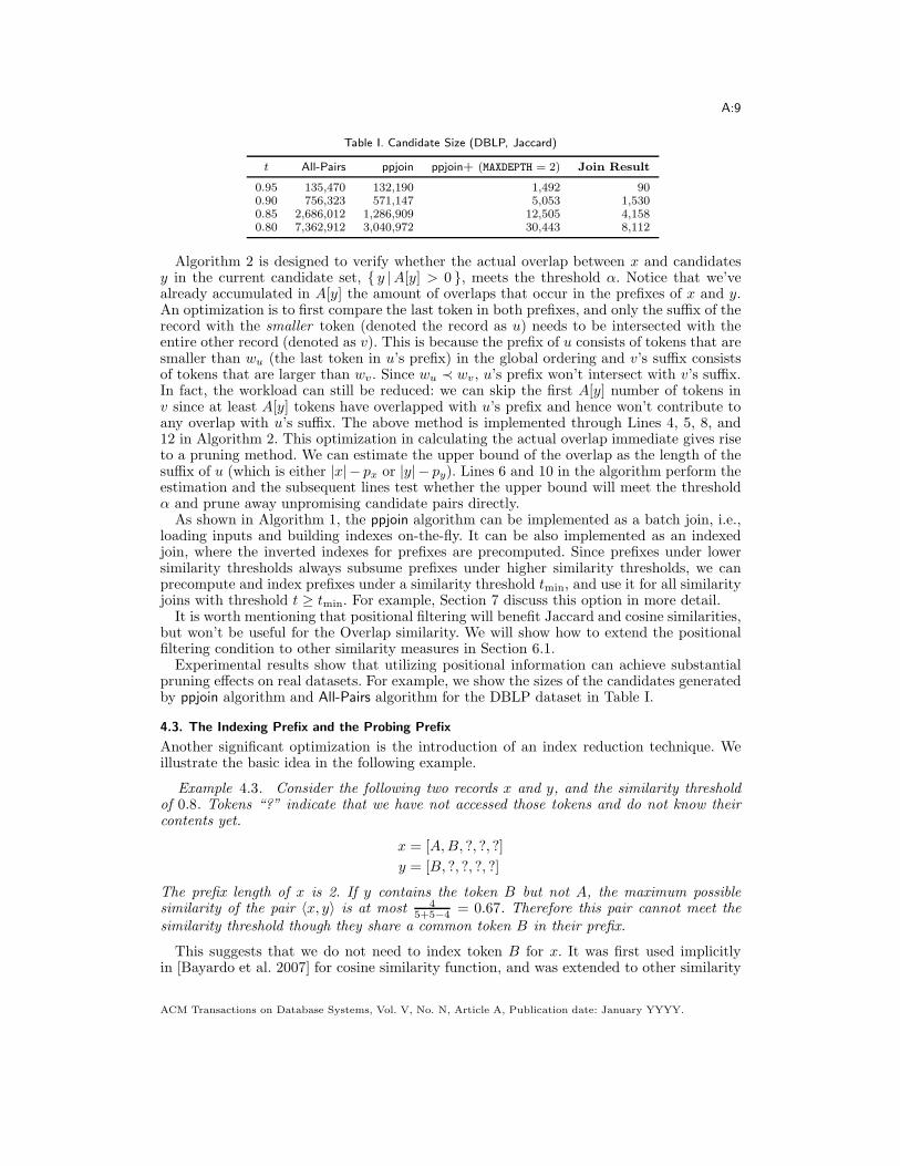
Table I. Candidate Size (DBLP, Jaccard)

t All-Pairs ppjoin ppjoin+ (MAXDEPTH = 2) Join Result

0.95 135,470 132,190 1,492 900.90 756,323 571,147 5,053 1,5300.85 2,686,012 1,286,909 12,505 4,1580.80 7,362,912 3,040,972 30,443 8,112

Algorithm 2 is designed to verify whether the actual overlap between x and candidatesy in the current candidate set, { y |A[y] > 0 }, meets the threshold α. Notice that we’vealready accumulated in A[y] the amount of overlaps that occur in the prefixes of x and y.An optimization is to first compare the last token in both prefixes, and only the suffix of therecord with the smaller token (denoted the record as u) needs to be intersected with theentire other record (denoted as v). This is because the prefix of u consists of tokens that aresmaller than wu (the last token in u’s prefix) in the global ordering and v’s suffix consistsof tokens that are larger than wv. Since wu ≺ wv, u’s prefix won’t intersect with v’s suffix.In fact, the workload can still be reduced: we can skip the first A[y] number of tokens inv since at least A[y] tokens have overlapped with u’s prefix and hence won’t contribute toany overlap with u’s suffix. The above method is implemented through Lines 4, 5, 8, and12 in Algorithm 2. This optimization in calculating the actual overlap immediate gives riseto a pruning method. We can estimate the upper bound of the overlap as the length of thesuffix of u (which is either |x| − px or |y| − py). Lines 6 and 10 in the algorithm perform theestimation and the subsequent lines test whether the upper bound will meet the thresholdα and prune away unpromising candidate pairs directly.As shown in Algorithm 1, the ppjoin algorithm can be implemented as a batch join, i.e.,

loading inputs and building indexes on-the-fly. It can be also implemented as an indexedjoin, where the inverted indexes for prefixes are precomputed. Since prefixes under lowersimilarity thresholds always subsume prefixes under higher similarity thresholds, we canprecompute and index prefixes under a similarity threshold tmin, and use it for all similarityjoins with threshold t ≥ tmin. For example, Section 7 discuss this option in more detail.It is worth mentioning that positional filtering will benefit Jaccard and cosine similarities,

but won’t be useful for the Overlap similarity. We will show how to extend the positionalfiltering condition to other similarity measures in Section 6.1.Experimental results show that utilizing positional information can achieve substantial

pruning effects on real datasets. For example, we show the sizes of the candidates generatedby ppjoin algorithm and All-Pairs algorithm for the DBLP dataset in Table I.

4.3. The Indexing Prefix and the Probing Prefix

Another significant optimization is the introduction of an index reduction technique. Weillustrate the basic idea in the following example.

Example 4.3. Consider the following two records x and y, and the similarity thresholdof 0.8. Tokens “?” indicate that we have not accessed those tokens and do not know theircontents yet.

x = [A,B, ?, ?, ?]

y = [B, ?, ?, ?, ?]

The prefix length of x is 2. If y contains the token B but not A, the maximum possiblesimilarity of the pair 〈x, y〉 is at most 4

5+5−4 = 0.67. Therefore this pair cannot meet thesimilarity threshold though they share a common token B in their prefix.

This suggests that we do not need to index token B for x. It was first used implicitlyin [Bayardo et al. 2007] for cosine similarity function, and was extended to other similarity


A:10

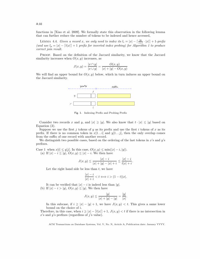
functions in [Xiao et al. 2009]. We formally state this observation in the following lemmathat can further reduce the number of tokens to be indexed and hence accessed,

Lemma 4.4. Given a record x, we only need to index its li = |x| − d 2t1+t· |x|e + 1-prefix

(and use lp = |x| − dt|x|e + 1 prefix for inverted index probing) for Algorithm 1 to producecorrect join result.

Proof. Based on the definition of the Jaccard similarity, we know that the Jaccardsimilarity increases when O(x, y) increases, as

J(x, y) =|x ∩ y||x ∪ y| =

O(x, y)

|x|+ |y| −O(x, y)

We will find an upper bound for O(x, y) below, which in turn induces an upper bound onthe Jaccard similarity.

Fig. 1. Indexing Prefix and Probing Prefix

Consider two records x and y, and |x| ≥ |y|. We also know that t · |x| ≤ |y| based onEquation (3).Suppose we use the first j tokens of y as its prefix and use the first i tokens of x as its

prefix. If there is no common token in x[1 . . i] and y[1 . . j], then the only overlap comesfrom the suffix of one record with another record.We distinguish two possible cases, based on the ordering of the last tokens in x’s and y’s

prefixes.

Case 1 when x[i] ≤ y[j]. In this case, O(x, y) ≤ min(|x| − i, |y|).(a) If |x| − i ≤ |y|, O(x, y) ≤ |x| − i. We then have

J(x, y) ≤ |x| − i

|x|+ |y| − |x|+ i≤ |x| − i

t|x|+ i.

Let the right hand side be less than t, we have

|x| − i

|x|+ i< t⇐⇒ i > (1− t)|x|.

It can be verified that |x| − i is indeed less than |y|.(b) If |x| − i > |y|, O(x, y) ≤ |y|. We then have

J(x, y) ≤ |y||x|+ |y| − |y| =

|y||x| .

In this subcase, if i ≥ |x| − |y| + 1, we have J(x, y) < t. This gives a same lowerbound on the choice of i.

Therefore, in this case, when i ≥ |x| − dt|x|e+1, J(x, y) < t if there is no intersection inx’s and y’s prefixes (regardless of j’s value).


A:11

Case 2 when x[i] > y[j]. In this case, O(x, y) ≤ min(|y| − j, |x|) = |y| − j.We then have

J(x, y) ≤ |y| − j

|x|+ |y| − |y|+ j≤ |y| − j

|y|+ j.

Let the right hand side less than t, we have

|y| − j

t|y|+ j< t⇐⇒ j >

1− t

1 + t|y|.

Therefore, in this case, when j ≥ |y| − d 2t1+t|y|e+1, J(x, y) < t if there is no intersection

in x’s and y’s prefixes (regardless of i’s value).

Remark 4.5. The root of this improvement comes from (1) the fact that records aresorted in increasing order of lengths (thus we can only use indexing prefix for short recordsand probing prefix for longer record) and (2) the fact that Jaccard similarity is relative tothe sizes of both records.

Remark 4.6. The above prefixes lengths are for the worst case scenario and are not tightotherwise, however, our positional filtering effectively removes all the spurious candidatesby taking the actual value of x and y (and is thus optimal if only this information is given).

We may extend the prefix length by k tokens, and then require a candidate pair havingno less than k + 1 common tokens.

Corollary 4.7. Consider using a li + k indexing prefix and lp + k probing prefix. Iftwo records do not have at least k+1 common tokens in their respective prefixes, the Jaccardsimilarity between them is less than t.

This optimization requires us to change Line 15 in Algorithm 1 such that it only indexesthe current token w if the current token position i is no larger than |x| − d 2t

1+t· |x|e+ 1.

In order not to abuse the term “prefix”, we denote “prefix” by default probing prefix inlater sections unless otherwise specified. We also exclude the the optimization using indexingprefixes for the ease of illustration in later sections, but integrate it into the implementationsin our experiments.

5. SUFFIX FILTERING

In this section, we first motivate the need of additional filtering method, and then introducea divide-and-conquer based suffix filtering method, which is a generalization of the positionalfiltering to the suffixes of the records.

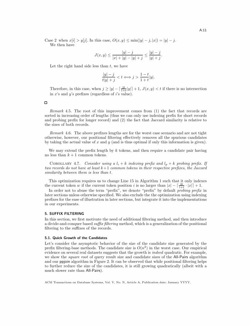
5.1. Quick Growth of the Candidates

Let’s consider the asymptotic behavior of the size of the candidate size generated by theprefix filtering-base methods. The candidate size is O(n2) in the worst case. Our empiricalevidence on several real datasets suggests that the growth is indeed quadratic. For example,we show the square root of query result size and candidate sizes of the All-Pairs algorithmand our ppjoin algorithm in Figure 2. It can be observed that while positional filtering helpsto further reduce the size of the candidates, it is still growing quadratically (albeit with amuch slower rate than All-Pairs).


A:12

0

500

1000

1500

2000

2500

3000

0.2 0.4 0.6 0.8 1S

quar

e R

oot o

f Can

dida

te S

ize

Scale Factor

DBLP, Jaccard Similarity, t = 0.80

All-PairsPPJoin

PPJoin+LSH-95%

Result

0

500

1000

1500

2000

2500

3000

0.2 0.4 0.6 0.8 1S

quar

e R

oot o

f Can

dida

te S

ize

Scale Factor


All-PairsPPJoin

PPJoin+LSH-95%

Result

Fig. 2. Quadratic Growth of Candidate Size

5.2. Generalization of Positional Filtering to Suffixes

Given the empirical observation about the quadratic growth rate of the candidate size, it isdesirable to find an additional pruning method in order to alleviate the problem and tacklereally large datasets.Our goal is to develop additional filtering method that prunes candidates that survive

the prefix and positional filtering. Our basic idea is to generalize the positional filteringprinciple to work on the suffixes of candidate pairs that survives after positional filtering,where the term “suffix” denotes the tokens not included in the prefix of a record. However,the challenge is that the suffixes of records are not indexed nor their partial overlap hasbeen calculated. Therefore, we face the following two technical issues: (i) how to establishan upper bound in the absence of indexes or partial overlap results? (ii) how to find positionof a token without tokens being indexed?We solve the first issue by converting an overlap constraint to an equivalent Hamming

distance constraint, according to Equation (2). We then lower bound the Hamming distanceby partitioning the suffixes in a coordinated way. We denote the suffix of a record x asxs. Consider a pair of records, 〈x, y〉, that meets the Jaccard similarity threshold t, andwithout loss of generality, |y| ≤ |x|. We can derive the following upper bound in terms ofthe Hamming distance of their suffixes:

H(xs, ys) ≤ Hmax =2|y| − 2d t

1 + t· (|x|+ |y|)e − (dt · |y|e − dt · |x|e). (5)

Proof. According to Jaccard similarity, the overlap between x and y is at least t1+t·

(|x|+ |y|). Therefore the Hamming distance of x and y

H(x, y) ≤ |x|+ |y| − 2d t

1 + t· (|x| + |y|)e.

The Hamming distance between x’s and y’s prefixes is at least the difference of the lengthsof the two prefixes, i.e.,

H(xp, yp) ≥ b((1 − t) · |x|+ 1)c − b((1 − t) · |y|+ 1)c,= b(1− t) · |x|c − b(1− t) · |y|c.

Therefore, we have

H(xs, ys) ≤ H(x, y)−H(xp, yp), = 2|y| − 2d t

1 + t· (|x|+ |y|)e − (dt · |y|e − dt · |x|e).


A:13

In order to check whether H(xs, ys) exceeds the maximum allowable value, we providean estimate of the lower bound of H(xs, ys) below. First we choose an arbitrary token wfrom ys, and divide ys into two partitions: the left partition yl and the right partition yr.The criterion for the partitioning is that the left partition contains all the tokens in ys thatprecede w in the global ordering and the right partition contains w (if any) and tokens inys that succeed w in the global ordering. Similarly, we divide xs into xl and xr using w too(even though w might not occur in x). Since xl (xr) shares no common token with yr (yl),H(xs, ys) = H(xl, yl) + H(xr, yr). The lower bound of H(xl, yl) can be estimated as thedifference between |xl| and |yl|, and similarly for the right partitions. Therefore,

H(xs, ys) ≥ abs(|xl| − |yl|) + abs(|xr | − |yr|).Finally, we can safely prune away candidates whose lower bound Hamming distance is

already larger than the allowable threshold Hmax.We can generalize the above method to more than one probing token and repeat the test

several times independently to improve the filtering rate. However, we will show that if theprobings are arranged in a more coordinated way, results from former probings can be takeninto account and make later probings more effective. We illustrate this idea in the examplebelow.

Example 5.1. Consider the following two suffixes of length 6. Cells marked with “?”indicate that we have not accessed those cells and do not know their contents yet.

1 2 3 4 5 6pos

? D ? ? F ?xs

xll xlr xr

? ? D F ? ?ys

yll ylr yr

Assume the allowable Hamming distance is 2. If we probe the 4th token in ys (“F”),we have the following two partitions of ys: yl = ys[1 . . 3] and yr = ys[4 . . 6]. Assuming amagical “partition” function, we can partition xs into xs[1 . . 4] and xs[5 . . 6] using F . Thelower bound of Hamming distance is abs(3 − 4) + abs(3 − 2) = 2.If we perform the same test independently, say, using the 3rd token of ys (“D”), the

lower bound of Hamming distance is still 2. Therefore, 〈x, y〉 is not pruned away.However, we can actually utilize the previous test result. The result of the second probing

can be viewed as a recursive partitioning of xl and yl into xll, xlr, yll, and ylr. Obviouslythe total absolute differences of the sizes of the three partitions from two suffixes is an lowerbound of their Hamming distance, which is

abs(|xll| − |yll|) + abs(|xlr | − |ylr|) + abs(|xr | − |yr|)= abs(1− 2) + abs(3 − 1) + abs(2 − 3) = 4.

Therefore, 〈x, y〉 can be safely pruned.

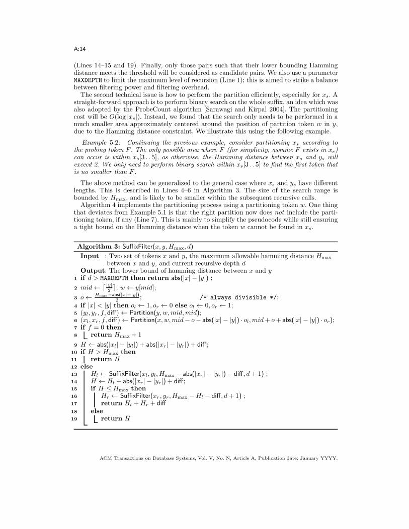
The algorithm we designed to utilize above observations is a divide-and-conquer one(Algorithm 3). First, the token in the middle of y is chosen, and x and y are partitionedinto two parts respectively. The lower bounds of Hamming distance on both left and rightpartitions are computed and summed up to judge if the overall hamming distance is withinthe allowable threshold (Line 9–10). Then we call the SuffixFilter function recursively firston the left and then on the right partitions (Lines 13–19). Probing results in the previoustests are used to help reduce the maximum allowable Hamming distance (Line 16) and tobreak the recursion if the Hamming distance lower bound has exceeded the threshold Hmax


A:14

(Lines 14–15 and 19). Finally, only those pairs such that their lower bounding Hammingdistance meets the threshold will be considered as candidate pairs. We also use a parameterMAXDEPTH to limit the maximum level of recursion (Line 1); this is aimed to strike a balancebetween filtering power and filtering overhead.The second technical issue is how to perform the partition efficiently, especially for xs. A

straight-forward approach is to perform binary search on the whole suffix, an idea which wasalso adopted by the ProbeCount algorithm [Sarawagi and Kirpal 2004]. The partitioningcost will be O(log |xs|). Instead, we found that the search only needs to be performed in amuch smaller area approximately centered around the position of partition token w in y,due to the Hamming distance constraint. We illustrate this using the following example.

Example 5.2. Continuing the previous example, consider partitioning xs according tothe probing token F . The only possible area where F (for simplicity, assume F exists in xs)can occur is within xs[3 . . 5], as otherwise, the Hamming distance between xs and ys willexceed 2. We only need to perform binary search within xs[3 . . 5] to find the first token thatis no smaller than F .

The above method can be generalized to the general case where xs and ys have differentlengths. This is described in Lines 4–6 in Algorithm 3. The size of the search range isbounded by Hmax, and is likely to be smaller within the subsequent recursive calls.Algorithm 4 implements the partitioning process using a partitioning token w. One thing

that deviates from Example 5.1 is that the right partition now does not include the parti-tioning token, if any (Line 7). This is mainly to simplify the pseudocode while still ensuringa tight bound on the Hamming distance when the token w cannot be found in xs.

Algorithm 3: SuffixFilter(x, y,Hmax, d)

Input : Two set of tokens x and y, the maximum allowable hamming distance Hmax

between x and y, and current recursive depth dOutput: The lower bound of hamming distance between x and y

1 if d > MAXDEPTH then return abs(|x| − |y|) ;2 mid← d |y|2 e; w ← y[mid];

3 o← Hmax−abs(|x|−|y|)2 ; /* always divisible */;

4 if |x| < |y| then ol ← 1, or ← 0 else ol ← 0, or ← 1;5 (yl, yr, f, diff)← Partition(y, w,mid,mid);6 (xl, xr, f, diff)← Partition(x,w,mid− o− abs(|x| − |y|) · ol,mid+ o+ abs(|x| − |y|) · or);7 if f = 0 then8 return Hmax + 1

9 H ← abs(|xl| − |yl|)+ abs(|xr| − |yr|)+ diff;10 if H > Hmax then11 return H12 else13 Hl ← SuffixFilter(xl, yl, Hmax − abs(|xr | − |yr|)− diff, d+ 1) ;14 H ← Hl + abs(|xr | − |yr|)+ diff;15 if H ≤ Hmax then16 Hr ← SuffixFilter(xr , yr, Hmax −Hl − diff, d+ 1) ;17 return Hl +Hr + diff18 else19 return H


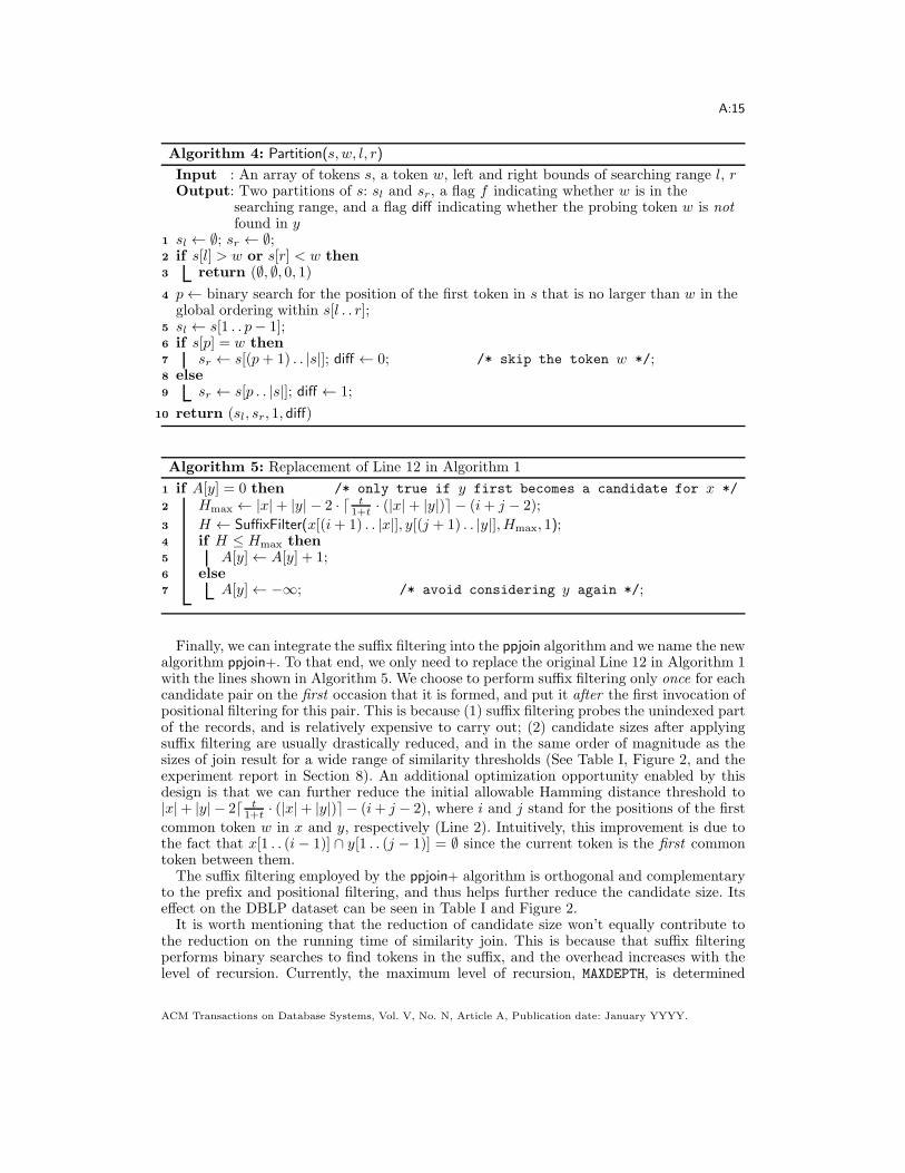
A:15

Algorithm 4: Partition(s, w, l, r)

Input : An array of tokens s, a token w, left and right bounds of searching range l, rOutput: Two partitions of s: sl and sr, a flag f indicating whether w is in the

searching range, and a flag diff indicating whether the probing token w is notfound in y

1 sl ← ∅; sr ← ∅;2 if s[l] > w or s[r] < w then3 return (∅, ∅, 0, 1)4 p← binary search for the position of the first token in s that is no larger than w in theglobal ordering within s[l . . r];

5 sl ← s[1 . . p− 1];6 if s[p] = w then7 sr ← s[(p+ 1) . . |s|]; diff ← 0; /* skip the token w */;8 else9 sr ← s[p . . |s|]; diff ← 1;

10 return (sl, sr, 1, diff)

Algorithm 5: Replacement of Line 12 in Algorithm 1

1 if A[y] = 0 then /* only true if y first becomes a candidate for x */

2 Hmax ← |x|+ |y| − 2 · d t1+t· (|x|+ |y|)e − (i+ j − 2);

3 H ← SuffixFilter(x[(i+ 1) . . |x|], y[(j + 1) . . |y|], Hmax, 1);4 if H ≤ Hmax then5 A[y]← A[y] + 1;6 else7 A[y]← −∞; /* avoid considering y again */;

Finally, we can integrate the suffix filtering into the ppjoin algorithm and we name the newalgorithm ppjoin+. To that end, we only need to replace the original Line 12 in Algorithm 1with the lines shown in Algorithm 5. We choose to perform suffix filtering only once for eachcandidate pair on the first occasion that it is formed, and put it after the first invocation ofpositional filtering for this pair. This is because (1) suffix filtering probes the unindexed partof the records, and is relatively expensive to carry out; (2) candidate sizes after applyingsuffix filtering are usually drastically reduced, and in the same order of magnitude as thesizes of join result for a wide range of similarity thresholds (See Table I, Figure 2, and theexperiment report in Section 8). An additional optimization opportunity enabled by thisdesign is that we can further reduce the initial allowable Hamming distance threshold to|x|+ |y| − 2d t

1+t· (|x|+ |y|)e − (i+ j − 2), where i and j stand for the positions of the first

common token w in x and y, respectively (Line 2). Intuitively, this improvement is due tothe fact that x[1 . . (i − 1)] ∩ y[1 . . (j − 1)] = ∅ since the current token is the first commontoken between them.The suffix filtering employed by the ppjoin+ algorithm is orthogonal and complementary

to the prefix and positional filtering, and thus helps further reduce the candidate size. Itseffect on the DBLP dataset can be seen in Table I and Figure 2.It is worth mentioning that the reduction of candidate size won’t equally contribute to

the reduction on the running time of similarity join. This is because that suffix filteringperforms binary searches to find tokens in the suffix, and the overhead increases with thelevel of recursion. Currently, the maximum level of recursion, MAXDEPTH, is determined


A:16

heuristically, as it depends on the data distribution and similarity threshold. We determineits optimal value by running the algorithm on a sample of the dataset with different valuesand choosing the one giving the best performance. A larger value of MAXDEPTH reduces thesize of the candidates to be verified, yet incurs overhead for the pruning. For all the datasetswe have tested, the optimal MAXDEPTH value ranges from 2 to 5. In Section 8.1.6, we willstudy the effect of the parameter MAXDEPTH using experimental evaluation to find the overallmost efficient algorithm.

6. EXTENSIONS

6.1. Extension to Other Similarity Measures

In this section, we briefly comment on necessary modifications to adapt both ppjoin andppjoin+ algorithms to other commonly used similarity measures. The major changes arerelated to the length of the prefixes used for indexing (Line 15, Algorithm 1) and used forprobing (Line 5, Algorithm 1), the threshold used by size filtering (Line 8, Algorithm 1) andpositional filtering (Line 9, Algorithm 1), and the Hamming distance threshold calculation(Line 2, Algorithm 5).

Overlap Similarity O(x, y) ≥ α is inherently supported in our algorithms. The prefixlength for a record x will be x−α+1. The size filtering threshold is α. It can be shown thatpositional filtering will not help pruning candidates, but suffix filtering is still useful. TheHamming distance threshold, Hmax, for suffix filtering will be |x|+ |y| − 2α− (i+ j − 2).

Edit Distance Edit distance is a common distance measure for strings. An edit distanceconstraint can be converted into weaker constraints on the overlap between the q-gram setsof the two strings. Specifically, let |u| be the length of the string u, a necessary condition fortwo strings to have less than δ edit distance is that their corresponding q-gram sets musthave overlap no less than α = (max(|u|, |v|) + q − 1)− qδ [Gravano et al. 2001].The prefix length of a record x (which is now a set of q-grams) is qδ+1. The size filtering

threshold is |x| − δ. Positional filtering will use an overlap threshold α = |x| − qδ. TheHamming distance threshold, Hmax, for suffix filtering will be |y| − |x|+ 2qδ − (i + j − 2).

Cosine Similarity We can convert a constraint on cosine similarity to an equivalentoverlap constraint as:

C(x, y) ≥ t⇐⇒ O(x, y) ≥⌈

t ·√

|x| · |y|⌉

The length of the prefix for a record x is |x| − dt2 · |x|e+ 1, yet the length of the tokensto be indexed can be optimized to |x| − dt · |x|e+1. The size filtering threshold is dt2 · |x|e.2Positional filtering will use an overlap threshold α =

⌈

t ·√

|x| · |y|⌉

. The Hamming distance

threshold, Hmax, for suffix filtering will be |x|+ |y| − 2⌈

t ·√

|x| · |y|⌉

− (i+ j − 2).

6.2. Generalization to the Weighted Case

To adapt the ppjoin and ppjoin+ algorithms to the weighted case, we mainly need to modifythe computation of the prefix length. In the following, we use weighted Jaccard similarity(defined below) as the example, and illustrate important changes.

Jw(x, y) =

∑

w∈|x∩y|weight(w)∑

w∈|x∪y|weight(w)

The binary Jaccard similarity we discussed before is just a special case when all the weightsare 1.0.

2These are the same bounds obtained in [Bayardo et al. 2007].


A:17

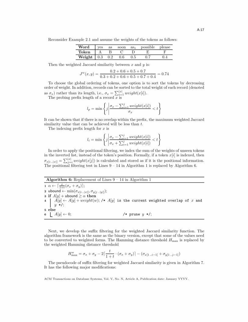
Reconsider Example 2.1 and assume the weights of the tokens as follows:

Word yes as soon as1 possible pleaseToken A B C D E FWeight 0.3 0.2 0.6 0.5 0.7 0.4

Then the weighted Jaccard similarity between x and y is:

Jw(x, y) =0.2 + 0.6 + 0.5 + 0.7

0.3 + 0.2 + 0.6 + 0.5 + 0.7 + 0.4= 0.74

To choose the global ordering of tokens, one option is to sort the tokens by decreasingorder of weight. In addition, records can be sorted to the total weight of each record (denoted

as σx) rather than its length, i.e., σx =∑|x|

i=1 weight(x[i]).The probing prefix length of a record x is

lp = min

{

j

∣

∣

∣

∣

∣

σx −∑j

i=1 weight(x[i])

σx

< t

}

It can be shown that if there is no overlap within the prefix, the maximum weighted Jaccardsimilarity value that can be achieved will be less than t.The indexing prefix length for x is

li = min

{

j

∣

∣

∣

∣

∣

σx −∑j

i=1 weight(x[i])

σx +∑j

i=1 weight(x[i])< t

}

In order to apply the positional filtering, we index the sum of the weights of unseen tokensin the inverted list, instead of the token’s position. Formally, if a token x[i] is indexed, then

σx[i ..|x|] =∑|x|

j=i weight(x[j]) is calculated and stored as if it is the positional information.The positional filtering test in Lines 9 – 14 in Algorithm 1 is replaced by Algorithm 6.

Algorithm 6: Replacement of Lines 9 – 14 in Algorithm 1

1 α← d t1+t

(σx + σy)e;2 ubound← min(σx[i ..|x|], σy[j ..|y|]);3 if A[y] + ubound ≥ α then4 A[y]← A[y] +weight(w); /* A[y] is the current weighted overlap of x and

y */;5 else6 A[y]← 0; /* prune y */;

Next, we develop the suffix filtering for the weighted Jaccard similarity function. Thealgorithm framework is the same as the binary version, except that some of the values needto be converted to weighted forms. The Hamming distance threshold Hmax is replaced bythe weighted Hamming distance threshold

Hwmax = σx + σy − 2d t

1 + t· (σx + σy)e − (σx[1 ..i−1] + σy[1 ..j−1])

The pseudocode of suffix filtering for weighted Jaccard similarity is given in Algorithm 7.It has the following major modifications:


A:18

Algorithm 7: SuffixFilterWeighted(x, y,Hwmax, d)

Input : Two set of tokens x and y, the maximum allowable weighted hammingdistance Hw

max between x and y, and current recursive depth dOutput: The lower bound of weighted hamming distance between x and y

1 if d > MAXDEPTH then2 if |x| ≥ |y| then3 return weight(x[|x|]) · (|x| − |y|)4 else5 return weight(y[|y|]) · (|y| − |x|)

6 mid← d |y|2 e; w ← y[mid];

7 o← d Hw

max

weight(w) e;8 (yl, yr, f, diff)← Partition(y, w,mid,mid);9 (xl, xr, f, diff)← Partition(x,w,mid− o,mid+ o);

10 if f = 0 then11 return Hw

max + 1

12 if |xl| ≥ |yl| then13 Hw

l ← weight(xl[|xl|]) · (|xl| − |yl|);14 else15 Hw

l ← weight(yl[|yl|]) · (|yl| − |xl|);16 if |xr | ≥ |yr| then17 Hw

r ← weight(xr[|xr |]) · (|xr| − |yr|);18 else19 Hw

r ← weight(yr[|yr|]) · (|yr| − |xr |);20 Hw ← Hw

l +Hwr + diff · weight(w);

21 if Hw > Hwmax then

22 return Hw

23 else24 Hw

l ← SuffixFilterWeighted(xl, yl, Hwmax −Hw

r − diff · weight(w), d+ 1) ;25 Hw ← Hw

l +Hwr + diff · weight(w);

26 if Hw ≤ Hwmax then

27 Hwr ← SuffixFilterWeighted(xr, yr, H

wmax −Hw

l − diff · weight(w), d+ 1) ;28 return Hw

l +Hwr + diff · weight(w)

29 else30 return Hw

— Lines 1 – 5 : If the recursive depth d is greater than MAXDEPTH, we compare the lengthof x and y, and select the longer one. Its last token has the least weight. The weight ismultiplied by the length difference of x and y, and then returned as a lower bound ofweighted hamming distance. Note that the inputs to the algorithm x and y can be not onlyrecords but also partitions, therefore we are unable to obtain the exact value of the weightedsum of x’s or y’s tokens unless it is calculated on-the-fly or is calculated beforehand. Wechoose to return the lower bound as this will save time and space costs, though the boundis generally not as tight as the exact value.— Lines 7 – 9 : New search ranges are used to perform binary search efficiently for

weighted cases.— Lines 12 – 20 : We estimate the lower bound within the left (or right) partition by

multiplying the weight of the last token in the longer partition and the length difference.


A:19

7. IMPLEMENTING SIMILARITY JOINS ON RELATIONAL DATABASE SYSTEMS

In this section, we discuss and compare several alternatives to implement the similarityjoin algorithms (All-Pairs, ppjoin, and ppjoin+) on relational database management systems.Such implementations are disk-based, and of interest to both academia [Gravano et al. 2001]and industry [Chaudhuri et al. 2006]. We focus on the case of self-join and discuss necessarymodifications to accommodate non-self-join at the end of this section.We consider an input relation R with the following schema:

CREATE TABLE R (rid INTEGER PRIMARY KEY ,len INTEGER ,toks VARRAY (2048)

);

where rid is the identifier of a record, len is the length of this record, and toks is avariable-length array of token identifiers sorted in the increasing df order.3

The naıve scheme can be implemented as the following SQL query:

SELECT R1.rid , R2.ridFROM R R1 , R R2WHERE R1.rid1 < R2.rid

AND SIM (R1.text , R2.text) >= t

where SIM is the similarity function implemented in UDF.It is prohibitively expensive for large datasets, partly because the query entails (almost

half of) a cross self join on R. Although this scheme can be improved by keeping track ofthe lengths of each record and imposing a length difference constraint in the query, it stillhas prohibitively high cost in practice.In order to implement the prefix-filtering in SQL, there are few alternatives, which will

be discussed below.

7.1. All-Pairs

In order to incorporate the prefix filtering, a prefix table, PrefixR, is generated from relationR, with the following schema:

CREATE TABLE PrefixR (rid INTEGER ,len INTEGER ,tid INTEGER ,PRIMARY KEY (tid , rid )

);

where rid is the identifier of a record, len is the length of a record, and tid is a tokenthat appears in the record identified by rid. Note that all tokens in a record are orderedby increasing df values and the prefix of appropriate length are recorded in the PrefixRtable. Note that, unlike our non-DBMS implementation, we do not require the input recordssorted on their lengths. Instead, length filtering in the SQL query automatically enforcessuch a constraint.If the similarity threshold is known in advance, we can have a precise prefix table, where

the (probing) prefix of length |x|−dt|x|e+1 is record in Table PrefixR. We consider genericversion in Section 8.2.The SQL queries can be conceptually divided into two parts: (a) generating the candidate

pairs and (b) verifying them.

3The maximum capacity of VARRAY can be adjusted accordingly or other appropriate attribute type forstrings can be used.


A:20

CREATE VIEW CANDSET ASSELECT DISTINCT PR1.rid AS rid1 , PR2 .rid As rid2FROM PrefixR PR1 , PrefixR PR2WHERE PR1.rid < PR2.rid

AND PR1.tid = PR2.tidAND PR1.len >= CEIL(t * PR2 .len)

SELECT R1.rid , R2.ridFROM R R1 , R R2, CANDSET CWHERE C.rid1 = R1.rid

AND C.rid2 = R2.ridAND VERIFY (R1.toks , R2.toks , t) = 1

This scheme results in significant improvement over the naıve scheme for two main rea-sons: the reduction of candidate set due to the prefix filtering, and the use of length filteringthat reduces the complexity of generating the candidates.We note that this scheme is similar to the scheme proposed in [Chaudhuri et al. 2006]

with the following difference:

— The main difference is the use of length filtering, which is not possible in [Chaudhuriet al. 2006] as they mainly consider the overlap constraint.— The rid order in our scheme implies the length order.

7.2. Implementing ppjoin and ppjoin+

To achieve the best performance, we need an enhanced version of the PrefixR table byincluding an additional attribute pos. The SQL is listed below:

CREATE TABLE PrefixR (rid INTEGER ,len INTEGER ,tid INTEGER ,pos INTEGER ,PRIMARY KEY (tid , rid)

);

ppjoin can be implemented as

1 CREATE VIEW CANDSET AS2 SELECT DISTINCT PR1.rid AS rid1 , PR2 .rid As rid23 FROM PrefixR PR1 , PrefixR PR24 WHERE PR1.rid < PR2.rid5 AND PR1.tid = PR2.tid6 AND PR1.len >= CEIL(t * PR2 .len)7 AND PR1.len - PR1.pos >= CEIL(PR1 .len * 2 * t / (1+t))8 AND DECODE ( SIGN((PR1 .len - PR1.pos) - (PR2.len - PR2 .pos )),9 -1,

10 (PR1.len - PR1.pos ),11 (PR2.len - PR2.pos )12 ) >=13 CEIL( (PR1.len + PR2 .len) * t / (1+t) );


AND C.rid2 = R2.ridAND VERIFY (R1.len , R1.toks , R2.len , R2.toks , t) = 1

Note that

— The positional filtering is implemented in Lines 8–13. A subtlty is that the positionalfiltering is only correct on the first common token in a candidate pair’s prefixes. However,this implementation does not affect the correctness of the algorithm.


A:21

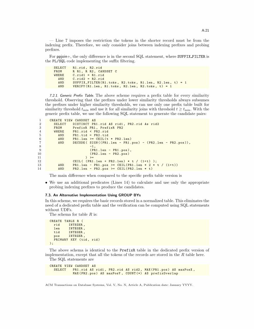
— Line 7 imposes the restriction the tokens in the shorter record must be from theindexing prefix. Therefore, we only consider joins between indexing prefixes and probingprefixes.

For ppjoin+, the only difference is in the second SQL statement, where SUFFIX FILTER isthe PL/SQL code implementing the suffix filtering.

SELECT R1.rid , R2.ridFROM R R1 , R R2 , CANDSET CWHERE C.rid1 = R1.rid

AND C.rid2 = R2.ridAND SUFFIX_FILTER(R1.toks , R2.toks , R1.len , R2.len , t) = 1AND VERIFY (R1.len , R1.toks , R2.len , R2.toks , t) = 1

7.2.1. Generic Prefix Table. The above scheme requires a prefix table for every similaritythreshold. Observing that the prefixes under lower similarity thresholds always subsumesthe prefixes under higher similarity thresholds, we can use only one prefix table built forsimilarity threshold tmin and use it for all similarity joins with threshold t ≥ tmin. With thegeneric prefix table, we use the following SQL statement to generate the candidate pairs:

1 CREATE VIEW CANDSET AS2 SELECT DISTINCT PR1 .rid AS rid1 , PR2.rid As rid23 FROM PrefixR PR1 , PrefixR PR24 WHERE PR1 .rid < PR2.rid5 AND PR1 .tid = PR2.tid6 AND PR1 .len >= CEIL(t * PR2.len )7 AND DECODE ( SIGN ((PR1.len - PR1 .pos) - (PR2.len - PR2.pos )),8 -1,9 (PR1 .len - PR1.pos),

10 (PR2 .len - PR2.pos)11 ) >=12 CEIL( (PR1.len + PR2.len ) * t / (1+t) );13 AND PR1 .len - PR1.pos >= CEIL(PR1.len * 2 * t / (1+ t))14 AND PR2 .len - PR2.pos >= CEIL(PR2.len * t)

The main difference when compared to the specific prefix table version is

• We use an additional predicates (Lines 14) to calculate and use only the appropriateprobing indexing prefixes to produce the candidates.

7.3. An Alternative Implementation Using GROUP BYs

In this scheme, we requires the basic records stored in a normalized table. This eliminates theneed of a dedicated prefix table and the verification can be computed using SQL statementswithout UDFs.The schema for table R is:

CREATE TABLE R (rid INTEGER ,len INTEGER ,tid INTEGER ,pos INTEGER ,PRIMARY KEY (tid , rid )

);

The above schema is identical to the PrefixR table in the dedicated prefix version ofimplementation, except that all the tokens of the records are stored in the R table here.The SQL statements are

CREATE VIEW CANDSET ASSELECT PR1 .rid AS rid1 , PR2.rid AS rid2 , MAX(PR1 .pos) AS maxPosX ,

MAX (PR2.pos) AS maxPosY , COUNT (*) AS prefixOverlap


A:22

FROM R PR1 , R PR2WHERE PR1.rid < PR2.rid

AND PR1.tid = PR2.tidAND PR1.len >= CEIL(t * PR2 .len)AND PR1.len - PR1.pos >= CEIL(PR1 .len * 2 * t / (1+t))AND PR2.len - PR2.pos >= CEIL(PR2 .len * t)AND DECODE ( SIGN((PR1 .len - PR1.pos) - (PR2.len - PR2 .pos )),

-1,(PR1.len - PR1.pos ),(PR2.len - PR2.pos )

) >=CEIL( (PR1.len + PR2 .len) * t / (1+t) )

GROUP BY PR1.rid , PR2.rid;


AND C.rid2 = R2.ridAND R1.tid = R2.tidAND R1.pos > maxPosXAND R2.pos > maxPosY

GROUP BY R1.rid , R2.ridHAVING COUNT (*) + prefixOverlap >=

(R1.len + R2.len) * t / (1+t) - C.cnt

Compared with the non-GROUP-BY implementation of the similarity join algorithms,the GROUP-BY implementation suffers from the fact that

— Positional filtering can only be applied after the GROUP BY operator.— The GROUP BY operator potentially has more overhead than the DISTINCT oper-

ator.

7.3.1. Using Longer Prefixes. We now consider using longer prefixes in the GROUP BYscheme. However, we use dedicated table to store longer prefixes here, but calculate theoverlap within the prefixes using GROUP BY clause. According to Corollary 4.7, we canindex extra k tokens in the PrefixR table, and then require a candidate pair having no lessthan k + 1 common tokens.For example, we implement ppjoin as

1 CREATE VIEW CANDSET AS2 SELECT PR1.rid AS rid1 , PR2 .rid As rid23 FROM PrefixR PR1 , PrefixR PR24 WHERE PR1.rid < PR2.rid5 AND PR1.tid = PR2.tid6 AND PR1.len >= CEIL(t * PR2 .len)7 AND PR1.len - PR1.pos >= CEIL(PR1 .len * 2 * t / (1+t)) - k8 AND PR2.len - PR2.pos >= CEIL(PR2 .len * t) - k9 AND DECODE ( SIGN((PR1 .len - PR1.pos) - (PR2.len - PR2 .pos )),

10 -1,11 (PR1.len - PR1.pos ),12 (PR2.len - PR2.pos )13 ) >=14 CEIL( (PR1.len + PR2 .len) * t / (1+t) ) - k;15 GROUP BY PR1.rid , PR2.rid16 HAVING COUNT (*) >= k + 1;


AND C.rid2 = R2.ridAND VERIFY (R1.len , R1.toks , R2.len , R2.toks , t) = 1


A:23

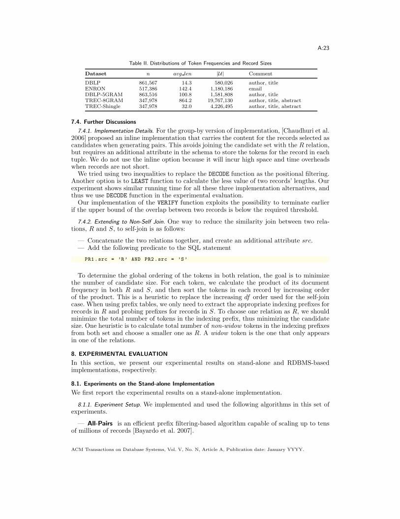
Table II. Distributions of Token Frequencies and Record Sizes

Dataset n avg len |U| Comment

DBLP 861,567 14.3 580,026 author, titleENRON 517,386 142.4 1,180,186 emailDBLP-5GRAM 863,516 100.8 1,581,808 author, titleTREC-8GRAM 347,978 864.2 19,767,130 author, title, abstractTREC-Shingle 347,978 32.0 4,226,495 author, title, abstract

7.4. Further Discussions

7.4.1. Implementation Details. For the group-by version of implementation, [Chaudhuri et al.2006] proposed an inline implementation that carries the content for the records selected ascandidates when generating pairs. This avoids joining the candidate set with the R relation,but requires an additional attribute in the schema to store the tokens for the record in eachtuple. We do not use the inline option because it will incur high space and time overheadswhen records are not short.We tried using two inequalities to replace the DECODE function as the positional filtering.

Another option is to LEAST function to calculate the less value of two records’ lengths. Ourexperiment shows similar running time for all these three implementation alternatives, andthus we use DECODE function in the experimental evaluation.Our implementation of the VERIFY function exploits the possibility to terminate earlier

if the upper bound of the overlap between two records is below the required threshold.

7.4.2. Extending to Non-Self Join. One way to reduce the similarity join between two rela-tions, R and S, to self-join is as follows:

— Concatenate the two relations together, and create an additional attribute src.— Add the following predicate to the SQL statement

PR1.src = ’R’ AND PR2 .src = ’S’

To determine the global ordering of the tokens in both relation, the goal is to minimizethe number of candidate size. For each token, we calculate the product of its documentfrequency in both R and S, and then sort the tokens in each record by increasing orderof the product. This is a heuristic to replace the increasing df order used for the self-joincase. When using prefix tables, we only need to extract the appropriate indexing prefixes forrecords in R and probing prefixes for records in S. To choose one relation as R, we shouldminimize the total number of tokens in the indexing prefix, thus minimizing the candidatesize. One heuristic is to calculate total number of non-widow tokens in the indexing prefixesfrom both set and choose a smaller one as R. A widow token is the one that only appearsin one of the relations.

8. EXPERIMENTAL EVALUATION

In this section, we present our experimental results on stand-alone and RDBMS-basedimplementations, respectively.

8.1. Experiments on the Stand-alone Implementation

We first report the experimental results on a stand-alone implementation.

8.1.1. Experiment Setup. We implemented and used the following algorithms in this set ofexperiments.

— All-Pairs is an efficient prefix filtering-based algorithm capable of scaling up to tensof millions of records [Bayardo et al. 2007].


A:24

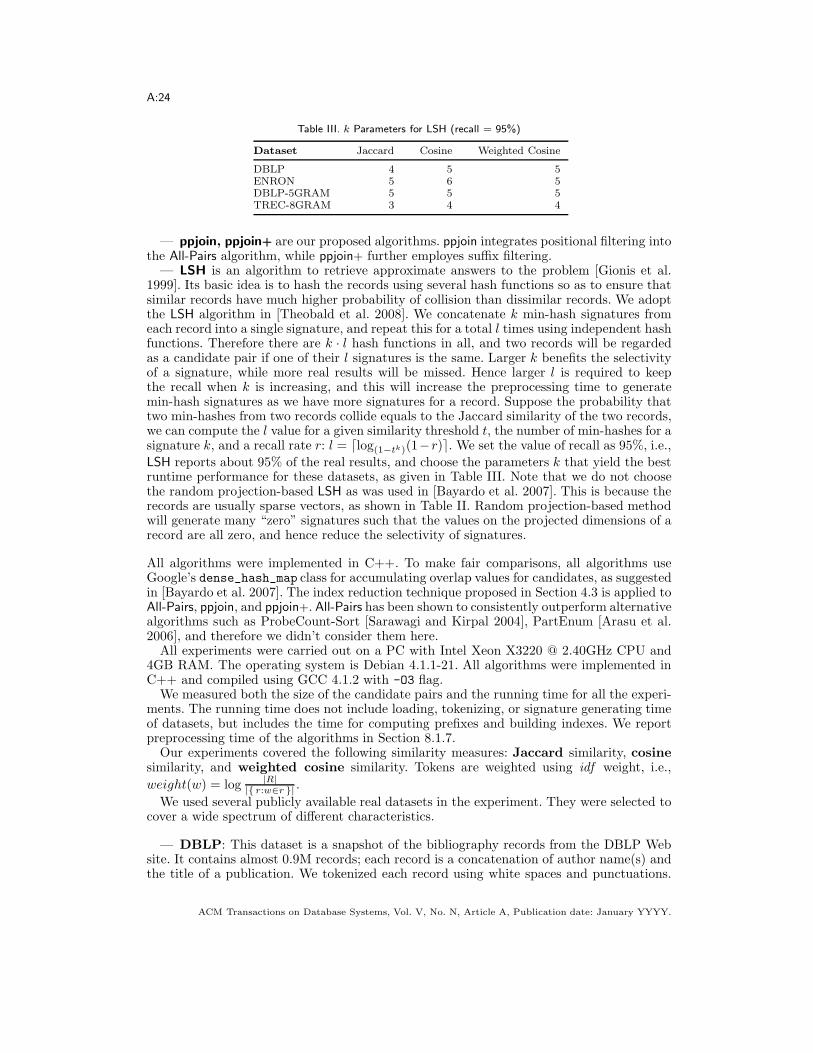
Table III. k Parameters for LSH (recall = 95%)

Dataset Jaccard Cosine Weighted Cosine

DBLP 4 5 5ENRON 5 6 5DBLP-5GRAM 5 5 5TREC-8GRAM 3 4 4

— ppjoin, ppjoin+ are our proposed algorithms. ppjoin integrates positional filtering intothe All-Pairs algorithm, while ppjoin+ further employes suffix filtering.— LSH is an algorithm to retrieve approximate answers to the problem [Gionis et al.

1999]. Its basic idea is to hash the records using several hash functions so as to ensure thatsimilar records have much higher probability of collision than dissimilar records. We adoptthe LSH algorithm in [Theobald et al. 2008]. We concatenate k min-hash signatures fromeach record into a single signature, and repeat this for a total l times using independent hashfunctions. Therefore there are k · l hash functions in all, and two records will be regardedas a candidate pair if one of their l signatures is the same. Larger k benefits the selectivityof a signature, while more real results will be missed. Hence larger l is required to keepthe recall when k is increasing, and this will increase the preprocessing time to generatemin-hash signatures as we have more signatures for a record. Suppose the probability thattwo min-hashes from two records collide equals to the Jaccard similarity of the two records,we can compute the l value for a given similarity threshold t, the number of min-hashes for asignature k, and a recall rate r: l = dlog(1−tk)(1−r)e. We set the value of recall as 95%, i.e.,

LSH reports about 95% of the real results, and choose the parameters k that yield the bestruntime performance for these datasets, as given in Table III. Note that we do not choosethe random projection-based LSH as was used in [Bayardo et al. 2007]. This is because therecords are usually sparse vectors, as shown in Table II. Random projection-based methodwill generate many “zero” signatures such that the values on the projected dimensions of arecord are all zero, and hence reduce the selectivity of signatures.

All algorithms were implemented in C++. To make fair comparisons, all algorithms useGoogle’s dense_hash_map class for accumulating overlap values for candidates, as suggestedin [Bayardo et al. 2007]. The index reduction technique proposed in Section 4.3 is applied toAll-Pairs, ppjoin, and ppjoin+. All-Pairs has been shown to consistently outperform alternativealgorithms such as ProbeCount-Sort [Sarawagi and Kirpal 2004], PartEnum [Arasu et al.2006], and therefore we didn’t consider them here.All experiments were carried out on a PC with Intel Xeon X3220 @ 2.40GHz CPU and

4GB RAM. The operating system is Debian 4.1.1-21. All algorithms were implemented inC++ and compiled using GCC 4.1.2 with -O3 flag.We measured both the size of the candidate pairs and the running time for all the experi-

ments. The running time does not include loading, tokenizing, or signature generating timeof datasets, but includes the time for computing prefixes and building indexes. We reportpreprocessing time of the algorithms in Section 8.1.7.Our experiments covered the following similarity measures: Jaccard similarity, cosine

similarity, and weighted cosine similarity. Tokens are weighted using idf weight, i.e.,

weight(w) = log |R||{ r:w∈r }| .

We used several publicly available real datasets in the experiment. They were selected tocover a wide spectrum of different characteristics.

— DBLP: This dataset is a snapshot of the bibliography records from the DBLP Website. It contains almost 0.9M records; each record is a concatenation of author name(s) andthe title of a publication. We tokenized each record using white spaces and punctuations.


A:25

The same DBLP dataset (with smaller size) was also used in previous studies [Arasu et al.2006; Bayardo et al. 2007; Xiao et al. 2008].— ENRON: This dataset is from the Enron email collection4. It contains about 0.5M

emails from about 150 users, mostly senior management of Enron. We tokenize the emailtitle and body into words using the same tokenization procedure as DBLP.— DBLP-5GRAM: This is the same DBLP dataset, but further tokenized into 5-grams.

Specifically, tokens in a record are concatenated with a single whitespace, and then every 5consecutive letters is extracted as a 5-gram.5

— TREC-8GRAM: This dataset is from TREC-9 Filtering Track Collections.6 It con-tains 0.35M references from the MEDLINE database. We extracted author, title, and ab-stract fields to from records. Every 8 consecutive letters is considered as an 8-gram.— TREC-Shingle: We applied Broder’s shingling method [Broder 1997] on TREC-

8GRAM to generate 32 shingles of 4 bytes per record, using min-wise independent permu-tations. TREC-8GRAM and TREC-Shingle are dedicated to experiment on near duplicateWeb page detection (Section 8.1.8).

Exact duplicates in the datasets are removed after tokenizing. The records are sorted intoincreasing length, and the tokens within each record are sorted into increasing documentfrequency. Some important statistics about the datasets are listed in Table II.

8.1.2. Jaccard Similarity.

Candidate Size Figures 3(a), 3(c), and 3(e) show the sizes of candidate pairs generated

by the algorithms and the size of the join result on the DBLP, Enron, and DBLP-5GRAMdatasets, with varying similarity thresholds from 0.80 to 0.95. Note that y-axis is in loga-rithm scale.Several observations can be made:

— The size of the join result grows modestly when the similarity threshold decreases.— All algorithms generate more candidate pairs with the decrease of the similarity

threshold. Obviously, the candidate size of All-Pairs grows the fastest. ppjoin has a decentreduction on the candidate size of All-Pairs, as the positional filtering prunes many candi-dates. ppjoin+ produces the fewest candidates among the three exact algorithms thanks tothe additional suffix filtering.— The candidate sizes of ppjoin+ are usually in the same order of magnitude as the

sizes of the join result for a wide range of similarity thresholds. The only outlier is Enrondataset, where ppjoin+ only produces modestly smaller candidate set than ppjoin. Thereare at least two reasons: (a) the average record size of the enron dataset is large; thisallows for a larger initial Hamming distance threshold Hmax for the suffix filtering. Yetwe only use MAXDEPTH = 2 (for efficiency reasons; also see the Enron’s true positive ratebelow). (b) Unlike other datasets used, an extraordinary high percentage of candidatesof ppjoin is join results. At the threshold of 0.8, the ratio of sizes of query result overcandidate size by ppjoin algorithm is 15.5%, 2.7%, and 0.02% for Enron, DBLP, and DBLP-5GRAM, respectively. In other words, ppjoin has already removed the majority of falsepositive candidate pairs on Enron and hence it is hard for suffix filtering to further reducethe candidate set.— LSH generates more candidates than All-Pairs and ppjoin under large threshold set-

tings, but fewer candidates than All-Pairs and ppjoin when small thresholds are applied. This

4Available at http://www.cs.cmu.edu/~enron/5According to [Xiao et al. 2008], long q-grams yield better performance than short q-grams onjoining long English text strings. Hence we use 5-grams on DBLP and 8-grams on TREC insteadof 3-grams and 4-grams, as were used in [Xiao et al. 2008].6Available at http://trec.nist.gov/data/t9_filtering.html.


A:26

101

102

103

104

105

106

107

108

0.8 0.85 0.9 0.95

Can

dida

te S

ize

Jaccard Similarity

DBLP

All-PairsPPJoin

PPJoin+LSH-95%

Result

(a) Jaccard, DBLP, Candidate Size

0

1

2

3

4

5

0.8 0.85 0.9 0.95

Tim

e (s

econ

ds)

Jaccard Similarity

DBLP

All-PairsPPJoin

PPJoin+LSH-95%

(b) Jaccard, DBLP, Time

106

107

108

0.8 0.85 0.9 0.95

Can

dida

te S

ize

Jaccard Similarity

ENRON

All-PairsPPJoin

PPJoin+LSH-95%

Result

(c) Jaccard, Enron, Candidate Size

0

5

10

15

20

25

30

35

40

0.8 0.85 0.9 0.95

Tim

e (s

econ

ds)

Jaccard Similarity

ENRON

All-PairsPPJoin

PPJoin+LSH-95%

(d) Jaccard, Enron, Time

103

104

105

106

107

108

109

0.8 0.85 0.9 0.95

Can

dida

te S

ize

Jaccard Similarity

DBLP-5GRAM

All-PairsPPJoin

PPJoin+LSH-95%

Result

(e) Jaccard, DBLP-5GRAM, Candidate Size

0

5

10

15

20

25

30

0.8 0.85 0.9 0.95

Tim

e (s

econ

ds)

Jaccard Similarity

DBLP-5GRAM

All-PairsPPJoin

PPJoin+LSH-95%

(f) Jaccard, DBLP-5GRAM, Time

Fig. 3. Experimental Results - Stand-alone Implementation (Jaccard)

is because when the threshold decreases, the tokens in the prefixes become more frequent,and thus the candidate sizes rapidly increase for algorithms based on prefix filtering. ForLSH, smaller thresholds only introduce more signatures while the selectivity remains almostthe same, and thus the candidate sizes do not increase as fast as All-Pairs and ppjoin. OnDBLP-5GRAM, LSH produces much fewer candidates than ppjoin. The main reason is thatthe q-grams are less selective then English words and even the rarest q-gram of a recordtends to be fairly frequent.

Running Time Figures 3(b), 3(d), and 3(f) show the running time of all algorithms onthe three datasets with varying Jaccard similarity thresholds.In all the settings, ppjoin+ is the most efficient exact algorithm7, followed by ppjoin. Both

algorithms outperform the All-Pairs algorithm. The general trend is that the speed-up in-creases with the decrease of the similarity threshold. This is because (a) index construction,

7Note that LSH is an approximate algorithm.


A:27

103

104

105

106

107

108

109

0.8 0.85 0.9 0.95

Can

dida

te S

ize

Cosine Similarity

DBLP

All-PairsPPJoin

PPJoin+LSH-95%

Result

(a) Cosine, DBLP, Candidate Size

0

5

10

15

20

25

0.8 0.85 0.9 0.95

Tim

e (s

econ

ds)

Cosine Similarity

DBLP

All-PairsPPJoin

PPJoin+LSH-95%

(b) Cosine, DBLP, Time

106

107

108

109

0.8 0.85 0.9 0.95

Can

dida

te S

ize

Cosine Similarity

ENRON

All-PairsPPJoin

PPJoin+LSH-95%

Result

(c) Cosine, Enron, Candidate Size

0

50

100

150

200

0.8 0.85 0.9 0.95

Tim

e (s

econ

ds)

Cosine Similarity

ENRON

All-PairsPPJoin

PPJoin+LSH-95%

(d) Cosine, Enron, Time

103

104

105

106

107

108

109

1010

0.8 0.85 0.9 0.95

Can

dida

te S

ize

Cosine Similarity

DBLP-5GRAM

All-PairsPPJoin

PPJoin+LSH-95%

Result

(e) Cosine, DBLP-5GRAM, Candidate Size

0

20

40

60

80

100

120

140

160

0.8 0.85 0.9 0.95

Tim

e (s

econ

ds)

Cosine Similarity

DBLP-5GRAM

All-PairsPPJoin

PPJoin+LSH-95%

(f) Cosine, DBLP-5GRAM, Time

Fig. 4. Experimental Results - Stand-alone Implementation (Cosine)

probing, and other overheads are more noticeable with a high similarity threshold, as theresult is small and easy to compute. (b) inverted lists in the indexes are longer for a lowersimilarity threshold; this increases the candidate size which in turn slows down the All-Pairsalgorithm as it does not have any other additional filtering mechanism. In contrast, manycandidates are quickly discarded by failing the positional or suffix filtering used in ppjoinand ppjoin+ algorithms.The speed-up that our algorithms can achieve against the All-Pairs algorithm is also

dependent on the dataset. At the 0.8 threshold, ppjoin can achieve 1.7x speed-up againstAll-Pairs on Enron, 1.4x on DBLP and DBLP-5GRAM. At the same threshold, ppjoin+ canachieve 1.8x speed-up on DBLP-5GRAM, 2x on DBLP, and 1.6x on Enron.The performance between ppjoin and ppjoin+ is most substantial on DBLP-5GRAM,

where filtering on the suffixes helps to improve the performance drastically. The reasonwhy ppjoin+ has only modest performance gain over ppjoin on Enron is because 16% ofthe candidates are final results, hence the additional filtering employed in ppjoin+ won’tcontribute to much runtime reduction. The difference of the two is also moderate on DBLP.


A:28

This is mainly because the average size of DBLP records is only 14 and even a brute-force verification using the entire suffix is likely to be fast, especially in modern computerarchitectures.Another important observation is that the improvement of positional filtering and suffix

filtering in overall running time is not so significant as the improvement in candidate size.There are two main factors: (a) The running time includes constructing inverted index andaccessing inverted lists to find candidates. ppjoin and ppjoin+ have no improvement in thesetwo procedures. (b) ppjoin+ prunes candidates with binary searches, and this overhead willincrease with the level of recursion, though the candidate size will be reduced.When compared with the approximate algorithm, ppjoin+ is 1.7x faster than LSH on

DBLP, and 3.2x faster on ENRON. LSH performs better on DBLP-5GRAM, and the speed-up can be up to 7.8x, as expected from the candidate sizes. This is again due to the poorselectivity of the q-grams.

8.1.3. Cosine Similarity. We ran all the algorithms on the DBLP, ENRON, and DBLP-5GRAM datasets using the cosine similarity function, and plot the candidate sizes in Fig-ures 4(a), 4(c), and 4(e) and running times in Figures 4(b), 4(d), and 4(f). For both metrics,the general trends are similar to those using Jaccard similarity. A major difference is that allalgorithms now run slower for the same similarity threshold, mainly because a cosine sim-ilarity constraint is inherently looser than the corresponding Jaccard similarity constraint.The speed-ups of the ppjoin and ppjoin+ algorithm can be up to 1.6x and 2.7x on DBLP,respectively; on Enron, the speed-ups are 1.5x and 1.6x, respectively; on DBLP-5GRAM,the speed-ups are 1.5x and 1.8x, respectively. On DBLP and ENRON, ppjoin+ is fasterthan LSH under high similarity thresholds, but slower when threshold is as low as 0.8. OnDBLP-5GRAM, LSH is always the most efficient algorithm, and gap is more significant thanthat on Jaccard similarity due to a looser constraint. This result demonstrates that LSH isa good choice under low threshold settings if not all the join results need to be reported.

8.1.4. Weighted Cosine Similarity. We run the four algorithms with weighted cosine similarityfunction on DBLP, ENRON, and DBLP-5RAM datasets. The candidate sizes are shown inFigures 5(a), 5(c), and 5(e); and the running times are shown in Figures 5(b), 5(d), and 5(f).Similar trends can be observed as those with Jaccard and cosine similarity functions. Allthe algorithms now run faster for the same similarity threshold than unweighted cosinesimilarity, since the tokens in the prefixes have more weights than those in the suffixes.Another important observation is that the speed-ups over All-Pairs algorithm are not asremarkable as with Jaccard or cosine similarity. This is because the tokens in prefixes areusually rare and assigned more weights; a candidate pair is then more likely to be a realresult, hence the problem itself becomes easier. For example, at the threshold of 0.8, theratio of real result size over candidate size by the All-Pairs algorithm increases by 4 times onall the three datasets when compared with unweighted case. With respect to the runningtime, ppjoin and ppjoin+ perform better than All-Pairs by a small margin, with a speed-up of1.2x and 1.3x on the three datasets, respectively. LSH is still slower than ppjoin+ on DBLP,but faster on DBLP-5GRAM. Like unweighted case, LSH is faster than ppjoin+ under lowthresholds on ENRON, but slower under high thresholds.

8.1.5. Varying Data Sizes. We performed the similarity join using Jaccard similarity on sub-sets of the DBLP dataset and measured running times.8 We randomly sampled about 20%to 100% of the records. We scaled down the data so that the data and result distributioncould remain approximately the same. We show the square root of the running time withJaccard similarity for the DLBP dataset and cosine similarity for the Enron dataset inFigures 6(a) and 6(b) (both thresholds are fixed at 0.8).

8We also measured the candidate sizes (e.g., see Figure 2).


A:29

103

104

105

106

107

108

0.8 0.85 0.9 0.95

Can

dida

te S

ize

Weighted Cosine Similarity

DBLP

All-PairsPPJoin

PPJoin+LSH-95%

Result

(a) Weighted Cosine, DBLP, Candidate Size

0

1

2

3

4

5

6

7

8

9

0.8 0.85 0.9 0.95

Tim

e (s

econ

ds)


DBLP

All-PairsPPJoin

PPJoin+LSH-95%

(b) Weighted Cosine, DBLP, Time

106

107

108

0.8 0.85 0.9 0.95

Can

dida

te S

ize


ENRON

All-PairsPPJoin

PPJoin+LSH-95%

Result

(c) Weighted Cosine, Enron, Candidate Size

5

10

15

20

25

30

35

40

45

50

0.8 0.85 0.9 0.95T

ime

(sec

onds

)Weighted Cosine Similarity

ENRON

All-PairsPPJoin

PPJoin+LSH-95%

(d) Weighted Cosine, Enron, Time

103

104

105

106

107

108

109

0.8 0.85 0.9 0.95

Can

dida

te S

ize


DBLP-5GRAM

All-PairsPPJoin

PPJoin+LSH-95%

Result

(e) Weighted Cosine, DBLP-5GRAM, Candidate Size

0

20

40

60

80

100

120

0.8 0.85 0.9 0.95

Tim

e (s

econ

ds)


DBLP-5GRAM

All-PairsPPJoin

PPJoin+LSH-95%

(f) Weighted Cosine, DBLP-5GRAM, Time

Fig. 5. Experimental Results - Stand-alone Implementation (Weighted Cosine)

0.6

0.8

1

1.2

1.4

1.6

1.8

2

0.2 0.4 0.6 0.8 1

Squ

are

Roo

t of T

ime

(sec

onds

)

Scale Factor


All-PairsPPJoin

PPJoin+LSH-95%

(a) Jaccard, DBLP, Time

0

2

4

6

8

10

12

14

0.2 0.4 0.6 0.8 1

Squ

are

Roo

t of T

ime

(sec

onds

)

Scale Factor

ENRON, Cosine Similarity, t = 0.80

All-PairsPPJoin

PPJoin+LSH-95%

(b) Cosine, Enron, Time

Fig. 6. Experimental Results - Stand-alone Implementation (Scalability)


A:30

It is clear that the running time of all the four algorithms grow quadratically. This isnot surprising given the fact that the actual result sizes already grows quadratically (e.g.,See Figure 2). Our proposed algorithms have demonstrated a slower growth rate than theAll-Pairs algorithm for both similarity functions and datasets.

8.1.6. Impacts of MAXDEPTH. An important tuning parameter of the ppjoin+ algorithm isMAXDEPTH, the maximum allowable recursion level while performing the suffix filtering. Wefound the following settings on MAXDEPTH work well empirically.

Dataset sim() MAXDEPTH

ANY Jaccard 2ANY Cosine 3

DBLP-5GRAM ANY 3 or 4

A possible explanation is that with a looser similarity function (e.g., cosine similarity)and/or longer records (e.g., DBLP-5GRAM), more probings are needed to achieve goodcandidate pruning effects, hence a larger MAXDEPTH works better.The reason why we do not use a large MAXDEPTH value is because the suffix filtering is

most effective in the initial several rounds of recursions. For example, we measured thecandidate sizes and running times of ppjoin + and list the result for DBLP-5GRAM usingJaccard similarity of 0.80 in Table IV.

Table IV. Impact of MAXDEPTH (DBLP-5GRAM, Jaccard, t = 0.8, Join Result Size = 9,041)

MAXDEPTH Candidate Size Time (secs)

0 16,268,451 21.4291 4,198,756 18.0112 557,258 16.6993 45,871 16.1574 16,404 16.2195 11,306 16.3076 9,675 16.4197 9,091 16.520

8.1.7. Preprocessing Time. We measured preprocessing cost for the algorithms. For variousalgorithms, the preprocessing time includes

— All-Pairs, ppjoin, and ppjoin+ extracting tokens and sorting by decreasing idf ;— LSH extracting tokens and generating min-hash signatures.

Note that All-Pairs and ppjoin+ have the same amount of preprocessing time as ppjoin. Thepreprocessing time for different algorithms is given in Table V.We observe that the preprocessing cost of ppjoin is lower than LSH on DBLP and ENRON,

but higher on the two q-gram datasets. Two factors may affect the preprocessing time ofppjoin: (a) the number of distinct tokens; (b) the average number of tokens in a record.The first factor affects the time to compute the global ordering of tokens, and the secondfactor affects the time to sort the array of token in each record. The preprocessing time

Table V. Preprocessing Time (Jaccard, t = 0.8, in secs)

Dataset All-Pairs, ppjoin, ppjoin+ LSH

DBLP 1.41 15.02ENRON 8.87 54.26DBLP-5GRAM 11.43 68.96TREC-8GRAM 61.69 72.14


A:31

Table VI. Overall Running Time (Jaccard, t = 0.8, in secs)

Dataset All-Pairs ppjoin ppjoin+ LSH

DBLP 5.71 4.45 3.59 17.55ENRON 40.14 33.45 28.56 78.78DBLP-5GRAM 40.53 32.87 27.58 71.04TREC-8GRAM 119.32 90.76 88.70 74.37

of LSH is determined by the choosing of parameters k and l. Larger k or l will bringhigher preprocessing cost since there will be more min-hash signatures for a record. Thepreprocessing time of ppjoin is 6.0 to 10.7 times less than that of LSH on DBLP, ENRON,and DBLP-5GRAM, as they have either small token universe or small average record size(Table II). The advantage of ppjoin on TREC-8GRAM is not as substantial due to largertoken universe and longer records. Nevertheless, ppjoin is still more efficient than LSH interms of preprocessing time.Considering both preprocessing and join, the overall running time is shown in Table VI.

It can be observed that ppjoin and ppjoin+ outperform LSH on the first three datasets. Evenon TREC-8GRAM, LSH is marginally faster then ppjoin and ppjoin+.

8.1.8. Near Duplicate Web Page Detection. We also investigate a specific application of thesimilarity join: near duplicate Web page detection. A traditional method is based on per-forming approximate similarity join on shingles computed from each record [Broder et al.1997]. Later work proposed further approximations mainly to gain more efficiency at thecost of result quality.Instead, we designed and tested four algorithms that perform exact similarity join on

q-grams or shingles. (a) qp algorithm where we use the ppjoin+ algorithm to join directlyon the set of 8-grams of each record. (b) qa algorithm is similar to qp except that All-Pairsalgorithm is used as the exact similarity join algorithm. (c) ql algorithm where we use LSHalgorithm to join on the set of 8-grams with 95% of recall. (d) sp algorithm where we use theppjoin+ algorithm to join on the set of shingles. We use Broder’s shingling method [Broder1997] to generate shingles with min-wise independent permutations. Each record has 32shingles represented in 4-byte integers.The metrics we measured are: running times, precision and recall of the join result. Since

algorithm qp returns exact answer based on the q-grams of the records, its result is a goodcandidate for the correct set of near duplicate documents. Hence, we define precision andrecall as follows:

Precision =|Rsp ∩Rqp||Rsp|

Recall =|Rsp ∩Rqp||Rqp|

where Rx is the set of result returned by algorithm x.We show the results in Table VII with varying Jaccard similarity threshold values.

Table VII. Quality vs. Time Trade-off of Approximate and Exact Similarity Join

t Precision Recall timeqa timeqp timesp timeql

0.95 0.04 0.28 4.15 3.09 0.22 0.570.90 0.09 0.25 13.02 8.00 0.32 1.160.85 0.20 0.30 28.16 15.95 0.49 1.720.80 0.29 0.26 57.63 27.01 0.82 2.23

Several observations can be made

— Shingling-based methods will mainly suffer from low recalls in the result, meaning thatonly a small fraction of truly similar Web pages will be returned. We manually examined


A:32

some similar pairs missing from Rsp (t = 0.95), and most of the sampled pairs are likely tobe near duplicates (e.g., they differ only by typos, punctuations, or additional annotations).Note that other variants of the basic shingling method, e.g., systematic sampling of shinglesor super-shingling [Broder et al. 1997] were designed to trade result quality for efficiency,and are most likely to have even worse precision and recall values.In contrast, exact similarity join algorithms (qp or qa) have the appealing advantage offinding all the near duplicates given a similarity function.— qp, while enjoying good result quality, requires longer running time. However, with

reasonably high similarity threshold (0.90+), qp can finish the join in less than 8 seconds.On the other hand, qa takes substantially longer time to perform the same join.— ql is very efficient to find the approximate answers to detect near duplicate Web

pages. The speed-up over exact algorithms is more substantial under low similarity thresholdsettings.— sp combines the shingling and ppjoin+ together and is extremely fast even for modest

similarity threshold of 0.80. This method is likely to offer better result quality than, e.g.,super-shingling, while still offering high efficiency.

In summary, ppjoin+ algorithm can be combined with q-grams or shingles to provideappealing alternative solutions to tackle the near duplicate Web page detection tasks. Wealso recommend users to choose LSH rather than shingling as an approximate solution forhigh recall purpose.

8.2. Experiments on the RDBMS-based Implementation

The main goal of this set of experiments is to compare the performance of various im-plementation alternative of similarity join algorithms on RDBMSs. We implemented thealgorithms discussed in Section 7 using a popular RDBMS.

8.2.1. Experiment Setup. The similarity measures used in the experiments are Jaccardsimilarity and Cosine similarity.

Table VIII. Statistics of Datasets

Dataset n avg len |U | Comment

DBLP 861,567 14.3 580,026 author, titleENRON 517,386 142.4 1,180,186 emailUNIREF-4GRAM 54,819 164.5 302,847 protein sequence

We used the following publicly available real datasets in the experiment.

— DBLP: This dataset is a snapshot of the bibliography records from the DBLP Website, as has been used in the experiment on stand-alone implementation in Section 8.1.— ENRON: This dataset is from the Enron email collection, as has been used in the

experiment on stand-alone implementation in Section 8.1.— UNIREF-4GRAM: It is the UniRef90 protein sequence data from the UniProt

project.9 We sampled 58K protein sequences from the original dataset; each sequence is anarray of amino acids coded as uppercase letters. Every 4 consecutive letters is then extractedas a 4-gram.

The records are sorted into increasing length, and the tokens within each record are sortedinto increasing document frequency. Some important statistics about the datasets are listedin Table VIII.

9http://beta.uniprot.org/ (downloaded in March, 2008)


A:33

8.2.2. Using the Generic Prefix Table. We first study the effect of using the generic prefixtable. We set tmin as 0.8 and use it for all similarity joins with threshold t ≥ tmin.Table IX shows the running time of the ppjoin algorithm on the DBLP dataset with

varying Jaccard similarity thresholds. Results for other datasets or algorithms are similar.

Table IX. Running Time (in secs) on DBLP

t Prefix Table Generic Prefix Table

0.95 22.793 23.8760.90 66.025 68.7730.85 143.657 146.1480.80 296.450 302.544

With respect to the running time, we observe that the implementation using the genericprefix table exhibits similar performance as that using the specific prefix table, though thelatter has a slight edge over the former under all the threshold settings. This suggests thatthe additional predicate that selects probing index prefixes from generic prefix table is notexpensive to compute when it is compared with the overall algorithm.Compared with specific prefix tables, generic prefix tables are more practical for many

applications. Hence we use generic prefix tables in the rest of the experiment.

8.2.3. Comparison with All-Pairs. We compare three algorithms, All-Pairs, ppjoin and ppjoin+,on the three datasets. We use Jaccard similarity function for DBLP and ENRON dataset,and Cosine similarity function for UNIREF dataset.Figures 7(a) – 7(c) show the running time of the three algorithms on the three datasets

with varying thresholds, where AP denotes All-Pairs, PP ppjoin, and PP+ ppjoin+.ppjoin algorithm is the most efficient of the three for all the settings. ppjoin+ is the

runner-up on DBLP and UNIREF-4GRAM, but the slowest on ENRON. The three algo-rithms exhibits similar performance when t is high, but the gap becomes significant when tdecreases. ppjoin achieves a speed-up of approximately 2x against All-Pairs on all the threedatasets. The reason why ppjoin+ performs worse than ppjoin is that suffix filtering is not soefficient under the RDBMS-base implementation, as the suffix filtering test is implementedusing a UDF. Another observation is that ppjoin+ is even slower than All-Pairs on ENRONdataset. This is because 38.1% of the candidate pairs are join results on ENRON, whereasthe percentage on DBLP and UNIREF is 4.9% and 0.002%. All-Pairs has already removeda majority of false positive candidates, and additional filtering is not helpful.For All-Pairs algorithm, the verification phase takes most of the running time, and the

percentage grows when t is decreasing. This is due to the large number of candidates pro-duced by All-Pairs algorithm, and the lack of any additional filtering technique to deal withthe increase of candidate pairs when t decreases. For ppjoin algorithm, most running timeis spent on generating candidate pairs when t is high, and the percentage reduces whent decreases. For example, generating candidate pairs takes 70% of the total running timewhen t is 0.95 on DBLP, while the percentage drops to 40% when t is 0.8. ppjoin+ algorithmspends most running time on generating candidate pairs, even when t is as low as 0.8. This isbecause (1) the number of candidates generated by ppjoin+ algorithm is close to the numberof real results, and thus the verification time is not as significant as for All-Pairs or ppjoin;(2) unlike under the stand-alone implementation, suffix filtering is not performed efficientlyunder DBMS implementations, and this contributes to the candidate pair generation time.On the ENRON dataset, candidate pair generating time of ppjoin+ algorithm is not as

dominant as on DBLP and UNIREF-4GRAM dataset. This is because a high percentage ofcandidate pairs are final results and the total number is quite large, and therefore verificationphase takes more running time.


A:34

0

100

200

300

400

500

600

AP PPPP+ AP PPPP+ AP PPPP+ AP PPPP+

0.8 0.85 0.9 0.95

Tim

e (s

econ

ds)

Jaccard

DBLP

VerificationCandidate Pair

(a) Jaccard, DBLP, Time

0

2000

4000

6000

8000

10000

12000


0.8 0.85 0.9 0.95

Tim

e (s

econ

ds)

Jaccard

ENRON


(b) Jaccard, Enron, Time

0

500

1000

1500

2000

2500

3000

3500


0.8 0.85 0.9 0.95

Tim

e (s

econ

ds)

Cosine

UNIREF-4GRAM


(c) Cosine, UNIREF-4GRAM, Time

0 50

100 150 200 250 300 350 400 450

GB DI GB DI GB DI GB DI

0.8 0.85 0.9 0.95

Tim

e (s

econ

ds)

Jaccard

DBLP


(d) Jaccard, DBLP, Time

103

104

105

106

107

0.8 0.85 0.9 0.95

Can

dida

te S

ize

Jaccard

DBLP

k = 0k = 1k = 2k = 3

(e) Jaccard, DBLP, Candidate Size

0

500

1000

1500

2000

2500

3000

3500

4000

k=0k=1k=2k=3 k=0k=1k=2k=3 k=0k=1k=2k=3 k=0k=1k=2k=3

0.8 0.85 0.9 0.95

Tim

e (s

econ

ds)

Jaccard

DBLP


(f) Jaccard, DBLP, Time

Fig. 7. Experimental Results - DBMS Implementation (I)

8.2.4. Comparison with the Implementation Using GROUP BYs. We compare two versions ofppjoin algorithm implementations using DISTINCT and GROUP BY operator, respectively.In addition, we also consider the implementation with longer prefixes. We report the resultson the DBLP dataset with the Jaccard similarity function.Figure 7(d) shows the running time of the algorithm implemented using distinct and

using group-by, where GB denotes GROUP-BY, and DI denotes DISTINCT.For the implementation using distinct, we use the generic prefix table, while the normal-

ized table is used for the implementation using group-by. The former is always faster thanthe latter, and the time ratio remains a steady value of 1.4 times.The implementation using group-by employs a normalized table rather than a generic

prefix table, and therefore the table for the join operator to generate candidate pairs hasmuch more number of rows than a dedicated prefix table. This increases the overhead of thecandidate pair generation, and hence affects the total running time. The implementationusing distinct also benefits from faster verification because the VERIFY function would returnearly as soon as the unseen part of the two records is unable to contribute enough overlap.


A:35

In contrast, the implementation using group-by has to perform an expensive group byoperation, with no early stop technique to facilitate the verification.To study the effect of longer prefixes, we perform experiment on the DBLP dataset

using the Jaccard similarity function and report the candidate size and running time inFigures 7(e) and 7(f).The candidate size is significantly reduced when we extend the standard prefix length by

one more token, but the reduction is less remarkable for further extending. This indicatesthat most candidate pairs that share only one token within the prefixes are not final results,but those sharing at least two common tokens within the extended prefixes have much morechance to become final results and are not easily to pruned by even longer prefixes.With respect to the running time, longer prefixes give worse overall performance. Extend-

ing prefix by one token is 1.8 times slower than using standard prefix, and the slow-downincreases to 4x and 11x when k = 2 and 3, respectively. The main reason is that the indexsize, i.e., the number of rows within the prefix table, increases with longer prefixes. Table Xshows the number of rows within the extended prefix table. For longer prefixes, we needto perform the join on a large table in order to generate candidate pairs, and hence moretime during the candidate generation phase. Moreover, longer prefixes admit more frequenttokens to the join operation, as the tokens within each record are sorted in the increasingdocument frequency order. This results in more pairs satisfying the join predicates beforecalling GROUP BY to filter them. The effect is more obvious when we further increase k,as can be seen from the drastically increase of the running time when we extend the prefixlength.

Table X. Using Longer Prefixes

k Number of Rows

0 2,956,6791 3,811,9452 4,667,2113 5,521,234

8.2.5. Comparison with PartEnum and LSH. We perform experiments to compare three al-gorithms, ppjoin, PartEnum, and LSH, and report the result on the DBLP dataset usingJaccard similarity. For PartEnum and LSH we use signature tables with respect to specificsimilarity thresholds, and choose the optimal parameter settings under various t. The num-ber of index entries10, candidate size and running time of the two algorithms are shown inFigures 8(a) – 8(c), where PartEnum is denoted as PE, and ppjoin as PP.ppjoin outperforms PartEnum and LSH under all the threshold settings, and the speed-up

is increasing with the decrease of similarity threshold. When t = 0.8, ppjoin is 29 timesfaster than PartEnum algorithm, and 2.4 times faster than LSH. There are two main factorscontributing to this result. First, ppjoin is smaller than the other two in index size. Whent is 0.8, ppjoin’s generic prefix table contains 3M rows, whereas LSH’s and PartEnum’ssignature tables have 4.3M and 15.6M rows, respectively. In spite of the fact that ppjoinhas an additional attribute of position included in the prefix to perform positional filtering,ppjoin still has the lowest cost in self-joining the prefix table. This explains why ppjoin ismore efficient than PartEnum and LSH in candidate generation. Second, the candidate sizeof PartEnum increases rapidly with the decrease of t, while ppjoin can achieve a moderateincrease, hence resulting in faster verification time. For example, the ratio of candidate sizebetween the two algorithms is 11.2 when t is 0.8. LSH also exhibits a moderate increase in

10As for the number of index entries for ppjoin algorithm, we mean the number of entries within the probingprefix with respect to specific t.


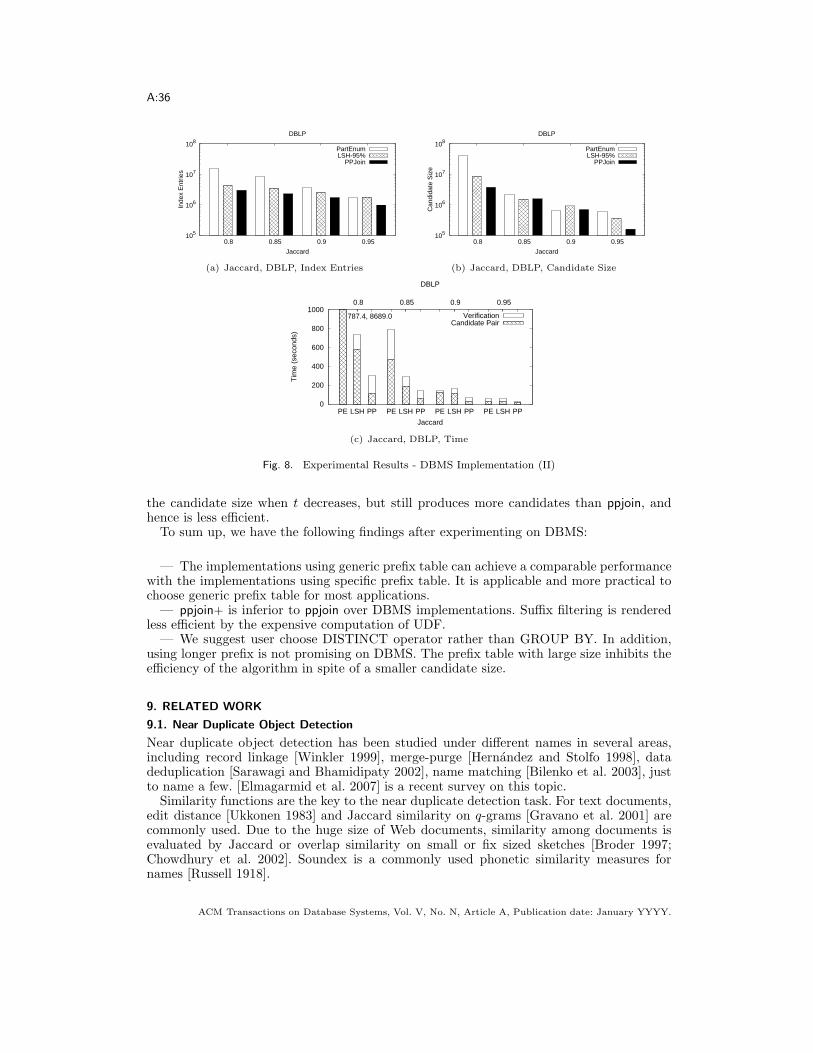
A:36

105

106

107

108

0.8 0.85 0.9 0.95

Inde

x E

ntrie

s

Jaccard

DBLP

PartEnumLSH-95%

PPJoin

(a) Jaccard, DBLP, Index Entries

105

106

107

108

0.8 0.85 0.9 0.95

Can

dida

te S

ize

Jaccard

DBLP

PartEnumLSH-95%

PPJoin

(b) Jaccard, DBLP, Candidate Size

0

200

400

600

800

1000

PE LSH PP PE LSH PP PE LSH PP PE LSH PP

0.8 0.85 0.9 0.95T

ime

(sec

onds

)

Jaccard

DBLP

787.4, 8689.0 VerificationCandidate Pair

(c) Jaccard, DBLP, Time

Fig. 8. Experimental Results - DBMS Implementation (II)

the candidate size when t decreases, but still produces more candidates than ppjoin, andhence is less efficient.To sum up, we have the following findings after experimenting on DBMS:

— The implementations using generic prefix table can achieve a comparable performancewith the implementations using specific prefix table. It is applicable and more practical tochoose generic prefix table for most applications.— ppjoin+ is inferior to ppjoin over DBMS implementations. Suffix filtering is rendered

less efficient by the expensive computation of UDF.— We suggest user choose DISTINCT operator rather than GROUP BY. In addition,

using longer prefix is not promising on DBMS. The prefix table with large size inhibits theefficiency of the algorithm in spite of a smaller candidate size.

9. RELATED WORK

9.1. Near Duplicate Object Detection

Near duplicate object detection has been studied under different names in several areas,including record linkage [Winkler 1999], merge-purge [Hernandez and Stolfo 1998], datadeduplication [Sarawagi and Bhamidipaty 2002], name matching [Bilenko et al. 2003], justto name a few. [Elmagarmid et al. 2007] is a recent survey on this topic.Similarity functions are the key to the near duplicate detection task. For text documents,

edit distance [Ukkonen 1983] and Jaccard similarity on q-grams [Gravano et al. 2001] arecommonly used. Due to the huge size of Web documents, similarity among documents isevaluated by Jaccard or overlap similarity on small or fix sized sketches [Broder 1997;Chowdhury et al. 2002]. Soundex is a commonly used phonetic similarity measures fornames [Russell 1918].


A:37

9.2. Exact Similarity Join and Near Duplicate Detection Algorithm

Existing methods for exact near duplicate detection usually convert constraints defined usingone similarity function into equivalent or weaker constraints defined on another similaritymeasure. [Gravano et al. 2001] converts edit distance constraints to overlap constraints onq-grams. Jaccard similarity constraints and 1/2-sided normalized overlap constraints canbe converted to overlap constraints [Sarawagi and Kirpal 2004; Chaudhuri et al. 2006; Xiaoet al. 2008]. Constraints on overlap, dice and Jaccard similarity measures can be convertedto constraints on cosine similarity [Bayardo et al. 2007]. [Arasu et al. 2006] transformsJaccard and edit distance constraints to Hamming distance constraints.The techniques proposed in previous work fall into two categories. In the first category,

exact near duplicate detection problems are addressed by inverted list based approaches[Bayardo et al. 2007; Chaudhuri et al. 2006; Sarawagi and Kirpal 2004], as discussed above.The second category of work [Arasu et al. 2006] is based on the pigeon hole principle. Therecords are carefully divided into partitions and then hashed into signatures, with whichcandidate pairs are generated, followed by a post-filtering step to eliminate false positives.[Arasu et al. 2008] designs a novel framework to identify similar records with some tokentransformations. In [Lieberman et al. 2008], LSS algorithm is proposed to perform similarityjoin using Graphics Processing Unit (GPU).Compared with [Xiao et al. 2008], we have made substantial improvements:

— We introduced an index reduction technique by illustrating the idea of using indexingprefixes.— We analyzed the prefix filtering technique.— We generalized ppjoin and ppjoin+ algorithms to several common similarity measures.— We proposed an optimized global ordering over the token universe to replace the

original increasing document frequency ordering.— We discussed and compared several alternatives to implement the similarity join al-

gorithms over relational database systems.

9.3. Approximate Near Duplicate Object Detection

Several previous work [Broder et al. 1997; Charikar 2002; Chowdhury et al. 2002; Gioniset al. 1999] has concentrated on the problem of retrieving approximate answers to similarityfunctions. LSH (Locality Sensitive Hashing) [Gionis et al. 1999] is a well-known approxi-mate algorithm for the problem. Its basic idea is to hash the records so that similar recordsare mapped to the same buckets with high probability. Broder et al. [Broder et al. 1997] ad-dressed the problem of identifying near duplicate Web pages approximately by compressingdocument records with a sketching function based on min-wise independent permutations.The near duplicate object detection problem is also a generalization of the well-known near-est neighbor problem, which is studied by a wide body of work, with many approximationtechniques considered by recent work [Charikar 2002; Fagin et al. 2003; Gionis et al. 1999;Indyk and Motwani 1998].

9.4. Similarity Join on Strings

The problem of similarity join on strings has been studied by several work [Gravano et al.2001; Xiao et al. 2008; 2008; Li et al. 2007; Yang et al. 2008].q-grams are widely used for approximate string match [Gravano et al. 2001]. It is especially

useful for edit distance constraints due to its ability to prune candidates with the countfiltering on q-grams. Together with prefix-filtering [Chaudhuri et al. 2006], the count filteringcan also be implemented efficiently. Filters based on mismatching q-grams are proposed tofurther speed up the query processing [Xiao et al. 2008].Gapped q-gram is shown to have better filtering powers than standard q-gram, but is

only suitable for edit distance threshold of 1 [Burkhardt and Karkkainen 2002]. A variable


A:38

length q-gram was proposed in [Li et al. 2007; Yang et al. 2008] and was shown to speed upmany computation tasks originally based on q-gram.Similarity join on strings is also closely related to approximate string matching, an ex-

tensively studied topic in algorithm and pattern matching communities. We refer readersto [Navarro 2001] and [Gusfield 1997].

9.5. Top-k Similarity Joins

The problem of top-k query processing has been studied by Fagin et al [Fagin 1999; Faginet al. 2003]. Much work build upon Fagin’s work for different application scenarios, e.g.,ranking query results from structured databases [Agrawal et al. 2003], processing distributedpreference queries [Chang and won Hwang 2002] and keyword queries [Luo et al. 2007].[Xiao et al. 2009] studies the top-k similarity join problem, which retrieves pairs of ob-

jects that have the highest similarity score among the data collection. Several optimizingtechniques are proposed by exploiting the monotonicity of similarity function and the or-der by which data are sorted. The indexing prefix was proposed to reduce both index andcandidate sizes.

9.6. Similarity Search

Several existing work studies the similarity search problem [Chaudhuri et al. 2003; Gravanoet al. 2001; Li et al. 2008; Hadjieleftheriou et al. 2008; Behm et al. 2009], which returns therecords in a collection whose similarity with the query exceeds a given threshold. Based onthe inverted list framework, [Li et al. 2008] proposes an efficient principle to skip recordswhen accessing inverted lists. For information retrieval(IR) purpose, [Hadjieleftheriou et al.2008] designs efficient techniques for indexing and processing similarity queries under IR-style similarity functions. [Behm et al. 2009] proposes a method to omitting some of thefrequent tokens while ensuring no true results are missed.

9.7. Document Fingerprinting

Another body of related work is document fingerprinting methods, mostly studied in thearea of document retrieval and World Wide Web.Shingling is a well-known document fingerprinting method [Broder 1997]. Shingles are

nothing but fixed length q-grams. All the shingles of a document are generated and only kshingles with the smallest hash values are kept. This process is repeated several times usingmin-wise independent hash functions. An alternative method is to use every l-th shingle orshingles that satisfy certain properties [Brin et al. 1995].Manber considered finding similar files in a file system [Manber 1994]. The scheme was

improved by Winnowing [Schleimer et al. 2003], which selects the q-gram whose hash valueis the minimum within a sliding window of q-grams. The Hailstorm method was proposedin [Hamid et al. 2009] which features the total coverage property, i.e., each token in thedocument is covered by at least one shingle. Another scheme based on DCT (DiscreteCosine Transformation) was proposed in [Seo and Croft 2008]. [Hamid et al. 2009] performeda comprehensive experimental comparison of some above-mentioned schemes.Charikar’s simhash [Charikar 2002] has been employed to detect near duplicates for Web

crawling [Manku et al. 2007]. After converting Web pages to high-dimensional vectors, itmaps the vectors to small-sized fingerprints. Near duplicates are identified by collecting thefingerprints that differ by only a few bits.There are also non-q-gram-based document fingerprinting methods. For example, I-

Match [Chowdhury et al. 2002] uses medium-document-frequency tokens as signatures.SpotSigs [Theobald et al. 2008] selects tokens around stopwords as signatures.


A:39

10. CONCLUSIONS

In this paper, we propose efficient similarity join algorithms by exploiting the ordering oftokens in the records. The algorithms provide efficient solutions for an array of applications,such as duplicate Web page detection on the Web. We show that positional filtering andsuffix filtering are complementary to the existing prefix filtering technique. They successfullyalleviate the problem of quadratic growth of candidate pairs when the size of data grows.We demonstrate the superior performance of our proposed algorithms to the existing prefixfiltering-based algorithms on several real datasets under a wide range of parameter settings.Experiments are also taken on relational databases to study several alternatives of algorithmimplementation. The proposed methods can also be adapted or integrated with existingnear duplicate Web page detection methods to improve the result quality or accelerate theexecution speed.

REFERENCES

Agrawal, S., Chaudhuri, S., Das, G., and Gionis, A. 2003. Automated ranking of database query results.In CIDR.

Arasu, A., Chaudhuri, S., and Kaushik, R. 2008. Transformation-based framework for record matching.In ICDE. 40–49.

Arasu, A., Ganti, V., and Kaushik, R. 2006. Efficient exact set-similarity joins. In VLDB.

Baeza-Yates, R. and Ribeiro-Neto, B. 1999. Modern Information Retrieval 1st Edition Ed. AddisonWesley.

Bayardo, R. J., Ma, Y., and Srikant, R. 2007. Scaling up all pairs similarity search. In WWW.

Behm, A., Ji, S., Li, C., and Lu, J. 2009. Space-constrained gram-based indexing for efficient approximatestring search. In ICDE. 604–615.

Bilenko, M., Mooney, R. J., Cohen, W. W., Ravikumar, P., and Fienberg, S. E. 2003. Adaptive namematching in information integration. IEEE Intelligent Sys. 18, 5, 16–23.

Brin, S., Davis, J., and Garcia-Molina, H. 1995. Copy detection mechanisms for digital documents. InSIGMOD Conference. 398–409.

Broder, A. Z. 1997. On the resemblance and containment of documents. In SEQS.

Broder, A. Z., Glassman, S. C., Manasse, M. S., and Zweig, G. 1997. Syntactic clustering of the web.Computer Networks 29, 8-13, 1157–1166.

Burkhardt, S. and Karkkainen, J. 2002. One-gapped q-gram filtersfor levenshtein distance. In CPM.225–234.

Chang, K. C.-C. and won Hwang, S. 2002. Minimal probing: supporting expensive predicates for top-kqueries. In SIGMOD Conference. 346–357.

Charikar, M. 2002. Similarity estimation techniques from rounding algorithms. In STOC.

Chaudhuri, S., Ganjam, K., Ganti, V., and Motwani, R. 2003. Robust and efficient fuzzy match foronline data cleaning. In SIGMOD Conference. 313–324.

Chaudhuri, S., Ganti, V., and Kaushik, R. 2006. A primitive operator for similarity joins in data cleaning.In ICDE.

Cho, J., Shivakumar, N., and Garcia-Molina, H. 2000. Finding replicated web collections. In SIGMOD.

Chowdhury, A., Frieder, O., Grossman, D. A., and McCabe, M. C. 2002. Collection statistics for fastduplicate document detection. ACM Trans. Inf. Syst. 20, 2, 171–191.

Conrad, J. G., Guo, X. S., and Schriber, C. P. 2003. Online duplicate document detection: signaturereliability in a dynamic retrieval environment. In CIKM.

Elmagarmid, A. K., Ipeirotis, P. G., and Verykios, V. S. 2007. Duplicate record detection: A survey.TKDE 19, 1, 1–16.

Fagin, R. 1999. Combining fuzzy information from multiple systems. J. Comput. Syst. Sci. 58, 1, 83–99.

Fagin, R., Kumar, R., and Sivakumar, D. 2003. Efficient similarity search and classification via rankaggregation. In SIGMOD.

Fagin, R., Lotem, A., and Naor, M. 2003. Optimal aggregation algorithms for middleware. J. Comput.Syst. Sci. 66, 4, 614–656.

Fetterly, D., Manasse, M., and Najork, M. 2003. On the evolution of clusters of near-duplicate webpages. In LA-WEB.


A:40

Gibson, D., Kumar, R., and Tomkins, A. 2005. Discovering large dense subgraphs in massive graphs. InVLDB.

Gionis, A., Indyk, P., and Motwani, R. 1999. Similarity search in high dimensions via hashing. In VLDB.

Gravano, L., Ipeirotis, P. G., Jagadish, H. V., Koudas, N., Muthukrishnan, S., and Srivastava, D.2001. Approximate string joins in a database (almost) for free. In VLDB.

Gusfield, D. 1997. Algorithms on Strings, Trees, and Sequences. Computer Science and ComputationalBiology. Cambridge University Press.

Hadjieleftheriou, M., Chandel, A., Koudas, N., and Srivastava, D. 2008. Fast indexes and algorithmsfor set similarity selection queries. In ICDE. 267–276.

Hamid, O. A., Behzadi, B., Christoph, S., and Henzinger, M. R. 2009. Detecting the origin of textsegments efficiently. In WWW. 61–70.

Henzinger, M. R. 2006. Finding near-duplicate web pages: a large-scale evaluation of algorithms. In SIGIR.

Hernandez, M. A. and Stolfo, S. J. 1998. Real-world data is dirty: Data cleansing and the merge/purgeproblem. Data Mining and Knowledge Discovery 2, 1, 9–37.

Hoad, T. C. and Zobel, J. 2003. Methods for identifying versioned and plagiarized documents. JA-SIST 54, 3, 203–215.

Indyk, P. and Motwani, R. 1998. Approximate nearest neighbors: Towards removing the curse of dimen-sionality. In STOC.

Li, C., Lu, J., and Lu, Y. 2008. Efficient merging and filtering algorithms for approximate string searches.In ICDE. 257–266.

Li, C., Wang, B., and Yang, X. 2007. VGRAM: Improving performance of approximate queries on stringcollections using variable-length grams. In VLDB.

Lieberman, M. D., Sankaranarayanan, J., and Samet, H. 2008. A fast similarity join algorithm usinggraphics processing units. In ICDE. 1111–1120.

Luo, Y., Lin, X., Wang, W., and Zhou, X. 2007. SPARK: top-k keyword query in relational databases.In SIGMOD Conference. 115–126.

Manber, U. 1994. Finding similar files in a large file system. In USENIX Winter. 1–10.

Manku, G. S., Jain, A., and Sarma, A. D. 2007. Detecting near-duplicates for web crawling. In WWW.141–150.

Navarro, G. 2001. A guided tour to approximate string matching. ACM Comput. Surv. 33, 1, 31–88.

Russell, R. C. 1918. Index, U.S. patent 1,261,167.

Sarawagi, S. and Bhamidipaty, A. 2002. Interactive deduplication using active learning. In KDD.

Sarawagi, S. and Kirpal, A. 2004. Efficient set joins on similarity predicates. In SIGMOD.

Schleimer, S., Wilkerson, D. S., and Aiken, A. 2003. Winnowing: Local algorithms for document fin-gerprinting. In SIGMOD Conference. 76–85.

Seo, J. and Croft, W. B. 2008. Local text reuse detection. In SIGIR. 571–578.

Spertus, E., Sahami, M., and Buyukkokten, O. 2005. Evaluating similarity measures: a large-scale studyin the orkut social network. In KDD.

Theobald, M., Siddharth, J., and Paepcke, A. 2008. Spotsigs: robust and efficient near duplicate detec-tion in large web collections. In SIGIR. 563–570.

Ukkonen, E. 1983. On approximate string matching. In FCT.

Winkler, W. E. 1999. The state of record linkage and current research problems. Tech. rep., U.S. Bureauof the Census.

Xiao, C., Wang, W., and Lin, X. 2008. Ed-Join: an efficient algorithm for similarity joins with edit distanceconstraints. PVLDB 1, 1, 933–944.

Xiao, C., Wang, W., Lin, X., and Shang, H. 2009. Top-k set similarity joins. In ICDE. 916–927.

Xiao, C., Wang, W., Lin, X., and Yu, J. X. 2008. Efficient similarity joins for near duplicate detection.In WWW.

Yang, X., Wang, B., and Li, C. 2008. Cost-based variable-length-gram selection for string collections tosupport approximate queries efficiently. In SIGMOD Conference. 353–364.


a eﬃcient similarity joins for near duplicate detectionweiw/files/tods-ppjoin-final.pdf · a...

Documents