a distance-based fuzzy time series model for exchange rates forecasting

Expert Systems with Applications 36 (2009) 8107–8114

Contents lists available at ScienceDirect

Expert Systems with Applications

journal homepage: www.elsevier .com/locate /eswa

A distance-based fuzzy time series model for exchange rates forecasting

Yungho Leu *, Chien-Pang Lee, Yie-Zu JouDepartment of Information Management, National Taiwan University of Science and Technology, 43, Keelung Road, Section 4, Taipei 10607, Taiwan, ROC

a r t i c l e i n f o

Keywords:Distance-based fuzzy time seriesFuzzy time seriesExchange rate forecasting

0957-4174/$ - see front matter � 2008 Elsevier Ltd. Adoi:10.1016/j.eswa.2008.10.034

* Corresponding author.E-mail address: [email protected] (Y. Leu).

a b s t r a c t

Fuzzy time series model has been successfully employed in predicting stock prices and foreign exchangerates. In this paper, we propose a new fuzzy time series model termed as distance-based fuzzy time series(DBFTS) to predict the exchange rate. Unlike the existing fuzzy time series models which require exactmatch of the fuzzy logic relationships (FLRs), the distance-based fuzzy time series model uses the dis-tance between two FLRs in selecting prediction rules. To predict the exchange rate, a two factors dis-tance-based fuzzy time series model is constructed. The first factor of the model is the exchange rateitself and the second factor comprises many candidate variables affecting the fluctuation of exchangerates. Using the exchange rate data released by the Central Bank of Taiwan, we conducted several exper-iments on exchange rate forecasting. The experiment results showed that the distance-based fuzzy timeseries outperformed the random walk model and the artificial neural network model in terms of meansquare error.

� 2008 Elsevier Ltd. All rights reserved.

1. Introduction

Forecasting financial time series such as the stock prices or theexchange rates is important to the investors and the government. Agood forecasting of a financial time series requires strong domainknowledge and good analysis tools. Many well-established meth-ods, such as autoregressive (AR), autoregressive moving average(ARMA) and generalized autoregressive conditional heteroscedas-ticity (GARCH), have been successfully applied for financial fore-casting. However, there are some limitations on applying theexisting methods. For example, in applying ARMA method oneneeds to make sure that the residue is normally distributed. Re-cently, due to the advance in artificial intelligence, many research-ers have focused on developing computational intelligencemethods for forecasting financial time series. For example, Pandaand Narasimhan predicted the exchange rate of Rupee and US dol-lar by artificial neural networks (Panda & Narasimhan, 2007). Caoet al. used support vector machines to predict the USD/GBP ex-change rate (Cao, Pang, & Bai, 2005). Shin and Han proposed anintegrated approach (Shin & Han, 2000) which uses genetic algo-rithms to choose the correct threshold parameters for wavelet soas to produce significant signal for a neural network. The inte-grated approach was used to predict the exchange rate of Koreanwon/US dollar. The fuzzy time series method is one of the compu-tational intelligence methods that draw much attention today. TheFuzzy time series model was first proposed by Song and Chissom(1993a, 1993b). Since then, many fuzzy time series models have

ll rights reserved.

been developed for forecasting index prices (Cheng, Chen, Teoh,& Chiang, 2008; Lee, Wang, Chen, & Leu, 2006; Yu, 2005) andenrollment of universities (Chen, 1996, 2002; Song & Chissom,1993a, 1993b). Recently, many extensions on fuzzy time serieshave been proposed. For example, Lee et al. (2006) proposed to al-low more than one factor in a fuzzy time series to improve theforecasting accuracy. Yu (2005) proposed to assign differentweights on fuzzy logic relationships (FLRs) based on their recency.The weights on fuzzy logic relationships are then used in defuzzifi-cation to determine the forecasted value of TAIEX.

The existing models for exchange rate forecasting use only thehistorical exchange rate itself to build the forecasting model. How-ever, according to the literatures, there are many factors that affectthe exchange rate of two currencies. For example, government pol-icies, expectations of the investors, and the stock indices are allshown to affect the fluctuation of the exchange rate (Benjamin,2006; Nieh & Lee, 2001). Thus, we propose to use the two-factorfuzzy time series to forecast the exchange rate. In an attempt touse the two-factor fuzzy time series model for exchange rate fore-casting, we found that it was very difficult to find matching rulesfor calculating the forecasted value. To remedy this shortcoming,we propose to extend the fuzzy time series model by using theEuclidean distance between two fuzzy logic relationships to findsimilar fuzzy logic relationships for calculating the forecasted va-lue. The new fuzzy time series model proposed in this paper istermed as distance-based fuzzy time series (DBFTS). DBFTS is atwo-factor high-order fuzzy time series model. The first factor ofDBFTS is the historical exchange rate, and the second factor com-prises several important variables that have an effect of on the ex-change rate.

mailto:[email protected]

http://www.sciencedirect.com/science/journal/09574174

http://www.elsevier.com/locate/eswa

8108 Y. Leu et al. / Expert Systems with Applications 36 (2009) 8107–8114

The contributions of this paper are threefold: (1) we propose touse the distance between two FLRs for selecting prediction ruleswhich makes the fuzzy time series model applicable for real lifeapplications in which the exact match of FLRs is not possible; (2)we propose to dynamically adjust the number of intervals of thesecond factor to improve the prediction accuracy;(3) we proposeto use PCA to derive the second factor, which allows incorporatingmultiple influential variables into the second factor.

The remainder of this paper is organized as follows. Section 2reviews several definitions of fuzzy time series models. Section 3introduces the DBFTS model. Section 4 presents the procedure ofusing DBFTS in exchange rate forecasting. In Section 5, we reportthe results of several experiments and compare the performanceof DBFTS, random walk model and RBFNN model in terms of meansquare error (MSE) and directional symmetry (DS). Finally, we con-clude this paper in Section 6.

2. Review of fuzzy time series models

According to the literature, the following definitions are givenfor fuzzy time series models.

Definition 1. Let Y(t) (t = . . .,0,1,2, . . .), a subset of R1, be theuniverse of discourse on which fuzzy sets fi(t) (i = 1,2, . . .) aredefined. If F(t) is a collection of fi(t). Then F(t) is called a fuzzy timeseries defined on Y(t).

Definition 2. If for any fj(t) 2 F(t), there exists an fi(t � 1) 2 F(t � 1),such that there exists a fuzzy relation Rij(t, t � 1) and fj(t) =fi(t � 1) � Rij(t, t � l) where ‘�’ is the max–min composition, thenF(t) is said to be caused by F(t � 1) only. Let R(t, t � 1)=[ijRij(t, t � 1) where ‘[’ is the union operator. Then R(t, t � 1) iscalled the fuzzy relation between F(t) and F(t � 1). We can writeF(t) = F(t � 1) � R(t, t � 1), and denote this as F(t � 1) ? F(t).

Definition 3. If F(t) is caused by F(t-1),F(t � 2), . . ., and F(t � n), F(t)is called a one-factor n-order fuzzy time series, and is denoted by

Fðt � nÞ; . . . ; Fðt � 2Þ; Fðt � 1Þ ! FðtÞ:

Based on the one-factor n-order fuzzy time series, Lee et al. (2006)proposed the two-factor high-order fuzzy time series as is definedin the following.

Definition 4. If F1(t) is caused by (F1(t � 1),F2(t � 1)),(F1(t�2),F2(t � 2)), . . ., (F1(t � n),F2(t � n)), F1(t) is called a two-fac-tor n-order fuzzy time series, which is denoted by

ðF1ðt � nÞ; F2ðt � nÞÞ; . . . ; ðF1ðt � 2Þ; F2ðt � 2ÞÞ; ðF1ðt � 1Þ; F2ðt � 1ÞÞ! F1ðtÞ:

Let F1(t) = Xt and F2(t) = Yt, where Xt and Yt are fuzzy sets on day t.Then, a two-factor n-order fuzzy relationship can be expressed as

ðXt�n;Yt�nÞ; . . . ; ðXt�2;Yt�2Þ; ðXt�1; Yt�1Þ ! Xt;

where (Xt�n,Yt�n), . . ., (Xt�2,Yt�2) and (Xt�1,Yt�1), are referred to asthe left-hand side (LHS) of the relationship, and Xt is referred toas the right-hand side (RHS) of the relationship. A fuzzy relationshipis also called a fuzzy logic relationship (FLR) in Chen (1996) andSong and Chissom (1993a, 1993b).

3. Distance-based fuzzy time series

As discussed in Section 1, the fluctuation of exchange rates in anexchange rate market is affected by many important variables. Inthe beginning, we employed the two-factor high-order fuzzy time

series proposed by Lee et al. (2006) to forecast the exchange ratesof Taiwan exchange rate market. Unfortunately, there are to toomany fuzzy sets at the LHS of an FLR, it was very difficult to finda matched FLR for predicting the exchange rate. This motivatesus to propose the DBFTS model which features in selecting fore-casting FLRs based on a distance metric defined on the LHS of anFLR, instead of a complete match of the LHS. The details of theDBFTS are explained in the following procedure. Note that differentfrom the Lee’s model, our approach contains two more steps fordetermining the second factor.

3.1. Step 1: Test of correlation coefficient

As defined in Definition 4, the first factor is caused by the firstand the second factors. Furthermore, the second factor may bederived from many candidate variables. To decide whether a can-didate variable is suitable for a component of the second factor,one has to test the correlation between the candidate variableand the first factor. If the correlation coefficient of the first factorand the candidate variable is not significant, the candidate vari-able should not be considered in the derivation of the secondfactor.

3.2. Step 2: Principal components analysis

After testing of correlation coefficient, the second factor canbe expressed as a linear combination of the candidate variablesthrough principal components analysis (PCA). For exchange rateforecasting, the second factor is the absolute score value of thefirst principal component, which is denoted by |PRIN1|. Note thatusually more than one component is needed for the secondfactor. However, for exchange rate forecasting, the first compo-nent has already explained 50–70% of the proportion of variance;we therefore choose only the first component as the secondfactor.

3.3. Step 3: Divide the universe of discourse

The universe of discourse of the first factor is defined asU = [Dmin � D1,Dmax + D2], where Dmin and Dmax are the minimumand maximum values of the first factor, respectively; D1 and D2

are two positive real numbers to divide the universe of discourseinto n equal length intervals (Song & Chissom, 1994). The universeof discourse of the second factor is defined as V = [Vmin � V1,Vmax + V2], where Vmin and Vmax are the minimum and maximumvalues of the second factor, respectively; V1 and V2 are two positivereal numbers used to divide the universe of discourse of the secondfactor into m equal length intervals.

3.4. Step 4: Define fuzzy sets

Linguistic term Ai, 1 6 i 6 n, is defined as a fuzzy set on theintervals of the first factor. Ai is defined as follows:

A1 ¼ 1=u1 þ 0:5=u2 þ 0=u3 þ � � � þ 0=un�2 þ 0=un�1 þ 0=un;

A2 ¼ 0:5=u1 þ 1=u2 þ 0:5=u3 þ � � � þ 0=un�2 þ 0=un�1 þ 0=un;

..

.

An�1 ¼ 0=u1 þ 0=u2 þ 0=u3 þ � � � þ 0:5=un�2 þ 1=un�1 þ 0:5=un;

An ¼ 0=u1 þ 0=u2 þ 0=u3 þ � � � þ 0=un�2 þ 0:5=un�1 þ 1=un:

Similarly, linguistic term Bj, 16 j 6m, is defined as a fuzzy set on theintervals of the second factor. Bj is defined as follows:

Y. Leu et al. / Expert Systems with Applications 36 (2009) 8107–8114 8109

B1 ¼ 1=v1 þ 0:5=v2 þ 0=v3 þ � � � þ 0=vm�2 þ 0=vm�1 þ 0=vm;

B2 ¼ 0:5=v1 þ 1=v2 þ 0:5=v3 þ � � � þ 0=vm�2 þ 0=vm�1 þ 0=vm;

..

.

Bm�1 ¼ 0=v1 þ 0=v2 þ 0=v3 þ � � � þ 0:5=vm�2 þ 1=vm�1 þ 0:5=vm;

Bm ¼ 0=v1 þ 0=v2 þ 0=v3 þ � � � þ 0=vm�2 þ 0:5=vm�1 þ 1=vm:

3.5. Step 5: Adjust the number of intervals of the second factor

Since the distance between two FLRs is used for rule selection,the number of intervals of the universes of discourse of the firstand the second factors plays an important role in selecting fore-casting rules. If the number of intervals of the first factor is muchgreater than that of the second factor, the first factor will dominatein selecting FLR forecasting rules; consequently, the forecast resultwill be primarily based on first factor. To balance the power inselecting forecast FLR rules, we adjust the number of intervals ofthe second factor to improve the forecasting accuracy.

3.6. Step 6: Fuzzification

Fuzzify the historical data of the first factor and the second fac-tor. An example of fuzzification is given in Section 4.

3.7. Step 7: Construct fuzzy logic relationships (FLR) database

For historical data on day i, let Xi�k, Yi�k denote the values ofF1(i � k) and F2(i � k) of the fuzzy time series, respectively, where1 6 k 6 n, and let Xi denote the value of F1(i). An FLR rule of the fuz-zy time series on day i can be represented as follows:

ðXi�n;Yi�nÞ; . . . ; ðXi�2;Yi�2Þ; ðXi�1;Yi�1Þ ! Xi:

3.8. Step 8: Forecast the first factor on day t

The value of the first factor on day t can be obtained through thefollowing procedure.

3.8.1. Construct the LHS of the FLR on day tConstruct the LHS of the FLR on day t and denote it as follows:

ðXt�n;Yt�nÞ; . . . ; ðXt�2;Yt�2Þ; ðXt�1;Yt�1Þ: ð1Þ

3.8.2. Search for similar FLRsCalculate the Euclidean distance (ED) between the LHS of the

FLR on day t and each LHS of a candidate FLRs in FLR database.Let ED denote the distance between the LHS on day t and theLHS of a candidate FLR rule on day i, then we have

ED ¼

ffiffiffiffiffiffiffiffiffiffiffiffiffiffiffiffiffiffiffiffiffiffiffiffiffiffiffiffiffiffiffiffiffiffiffiffiffiffiffiffiffiffiffiffiffiffiffiffiffiffiffiffiffiffiffiffiffiffiffiffiffiffiffiffiffiffiffiffiffiffiffiffiffiffiffiffiffiffiXn

j¼1

ððIXt�j � RXi�jÞ2 þ ðIYt�j � RYi�jÞ2vuut Þ; ð2Þ

where IXt�j and IYt�j are the subscripts of the fuzzy sets of the LHS ofday t’s FLR, respectively; that is, IXt�j is the subscript of fuzzy setXt�j and IYt�j is the subscript of fuzzy set Yt�j in formula (1). Simi-larly, RXi�j and RYi�j are the subscripts of their corresponding fuzzysets at the LHS of day i’s FLR.

Fig. 1. The framework of an artificial neural network.

3.8.3. Forecast the first factorTo forecast the value of the first factor on day t, we choose the

FLRs from FLR database with k smallest distances from the FLR onday t, and use the RHSs of these k FLRs to generate the forecast va-lue. The value of the first factor on day t can be calculated with thefollowing formula:

forecast value ¼ 1W

Xk

j¼1

1ED½j�M½j�; ð3Þ

where W ¼Pk

j¼11=ED½j�; ED[j] is the jth smallest Euclidean distance;M[j] is the midpoint value of the fuzzy set at the RHS of the FLR withthe jth smallest Euclidean distance. If ED[j] = 0 for any j where1 6 j 6 k, then the forecast_value is equal to the average of M[j]whose corresponding ED[j] equals 0.

4. Exchange rate forecasting

To study the performance of DBFTS, we compare it with the RWmodel and the RBFNN model in exchange rate forecasting. The RWmodel is deemed a simple and accurate model for financial timeseries (Meese & Rogoff, 1983), and the RBFNN model is a state-of-the-art model which is also used in financial time series fore-casting. We briefly review these two models in the following.

4.1. Random walk

Let St denote the exchange rate at time t. The random walkmodel for St can be written as

St ¼ St�1 þ et ; ð4Þ

where et is a white noise at time t satisfying E(et) = 0, var(et) = r2

and cov(et,es) = 0 for t – s. formula. (4) states that the exchange rateat time t is equal to the exchange rate at time t � 1 plus a whitenoise value at time t.

4.2. Artificial neural networks

The concept of artificial neural networks (ANN) was first intro-duced in 1950s. Since then many artificial neural network modelshave been proposed. Among them, the feedforward neural networkand the radial basis function neural network are most well-known.The framework of an artificial neural network, as shown in Fig. 1,contains three layers: the input layer, the hidden layer and the out-put layer. Since RBFNN model has been successfully applied inmany financial time series applications (Panda & Narasimhan,2007), we choose it as a target for comparison. We used the statis-tical software package R (R Project for Statistical Computing) tobuild an RBFNN model for exchange rate forecasting. In the RBFNNmodel, the input layer contains 3 nodes (one node for the exchangerate on day t � 3, day t � 2 and day t � 1, respectively); the hidden

Table 3Principal components analysis of the second factor.

Eigenvectors of the first principal component

JPY 0.463KRW 0.666CNY 0.118TAIEX �0.573


layer contains 4 nodes and the output layer contains a single nodefor the exchange rate (i.e., the forecasted exchange rate on day t).

4.3. Data

The NTD/USD, JPY/USD, CNY/USD and KRW/USD exchange ratesare collected from the website of the Central Bank of Taiwan, andthe Taiwan Stock Exchange Capitalization Weighted Stock Index(TAIEX) is collected from the website of the Taiwan Stock ExchangeCorporation. The exchange rates and TAIEX prices are the closeprices of each trading day. The experimental data comprise ex-change rates and TAIEX prices from March 1, 2006 to March 1,2007. Training data from March 1, 2006 to October 26, 2006 areused to construct FLR database for predicting the exchange rateon October 27, 2006. To predict the exchange rate on October 28,2006, we add the corresponding FLR on October 27, 2006 to theFLR database, and so on. The variables of the second factor areshown in Table 1. Note that due to the similarity in the economicstructures of Taiwan, China, Japan and South Korea, we chooseJPY/USD, CNY/USD and KRW/USD, along with TAIEX, as candidatevariables for the second factor.

4.4. Forecast exchange rates using the distance-based fuzzy time series

To demonstrate the way of using DBFTS in exchange rate fore-casting, we describe the procedure of forecasting the exchange rateof NTD/USD on October 27, 2006. Note that the exchange rates ofNTD/USD on the other days can be forecasted in a similar way.We have implemented DBFTS using statistical software packageR on a personal computer. The implemented program calls a sub-routine of R to perform the principal components analysis.

4.4.1. Step 1: Test of correlation coefficientTo decide whether a candidate variable is required for forecast-

ing NTD/USD, one has to test the correlation between the candidatevariable and NTD/USD. The results of the tests of correlation coef-ficients are shown in Table 2. Since the p values of all the tests aresignificant (at a significant level a = 0.05), all candidate variablesare required for NTD/USD.

4.4.2. Step 2: Principal components analysisThe second factor is created by inputting the training data into

R’s principal components analysis. The eigenvectors of the firstprincipal component are shown in Table 3. The second factor canbe written as

jPRIN1j ¼ j0:463 � JPY� þ 0:666 � KRW� þ 0:118 � CNY�

� 0:573 � TAIEX�j; ð5Þ

Table 1The candidate variables for the second factor.

Candidatevariable 1

Candidatevariable 2

Candidatevariable 3

Candidatevariable 4

The secondfactor

JPY/USD KRW/USD CNY/USD TAIEX

Table 2Correlation coefficients test.

Pearson correlation coefficients Prob > |r| under H0: Rho = 0

JPY/USD KRW/USD CNY/USD TAIEXNTD/USD <0.001 <0.001 <0.001 <0.001

Note: numbers in table are p value.

where JPY*, KRW*, CNY*, and TAIEX* are the values of JPY/USD, KRW/USD, CNY/USD, and TAIEX after normalization, respectively.

4.4.3. Step 3: Divide the universe of discourseLet U denote the universe of discourse of the first factor and V

denote the universe of discourse of the second factor. For forecast-ing the exchange rate on October 27, 2006, Dmin = 31.338, Dmax =33.316, D1 = 0 and D2 = 0.002; consequently, we have U =[31.338,33.318]. Similarly, we have Vmin = 0.01057013, Vmax =4.144669, V1 = 0, V2 = 0.0302023, and V = [0.01057013,4.14466920].

4.4.4. Step 4: Define fuzzy setsSince the minimum fluctuation of NTD/USD is 0.001 in the

training data set, the interval length of the first factor is set to0.005. Accordingly, the first factor is divided into 396 inter-vals, which are u1 = [31.338,31.343),u2 = [31.343,31.348), . . .,u396 = [33.313,33.318). The fuzzy sets of the first factor are repre-sented as follows:

A1 ¼ 1=u1 þ 0:5=u2 þ 0=u3 þ � � � þ 0=u394 þ 0=u395 þ 0=u396;

A2 ¼ 0:5=u1 þ 1=u2 þ 0:5=u3 þ � � � þ 0=u196 þ 0=u197 þ 0=u198;

..

.

A395 ¼ 0=u1 þ 0=u2 þ 0=u3 þ � � � þ 0:5=u394 þ 1=u395 þ 0:5=u396;

A396 ¼ 0=u1 þ 0=u2 þ 0=u3 þ � � � þ 0=u394 þ 0:5=u395 þ 1=u396:

Because the second factor is a linear combination of several vari-ables, it is not easy to choose an appropriate interval length. Instead,we decide the number of intervals first and then divide the universeof discourse evenly. To predict NTD/USD on October 27, 2006, weassume that the number of intervals of the second factor equals thatof the first factor. Consequently, the second factor is dividedinto 396 intervals, which are v1 = [0.01057013,0.02100977),v2 = [0.02100977,0.03144942), . . .,v396 = [4.13422955,4.14466920).The fuzzy sets of the second factor are represented as follows:

B1 ¼ 1=v1 þ 0:5=v2 þ 0=v3 þ � � � þ 0=v394 þ 0=v395 þ 0=v396;

B2 ¼ 0:5=v1 þ 1=v2 þ 0:5=v3 þ � � � þ 0=v394 þ 0=v395 þ 0=v396;

..

.

B395 ¼ 0=v1 þ 0=v2 þ 0=v3 þ � � � þ 0:5=v394 þ 1=v395 þ 0:5=v396;

B396 ¼ 0=v1 þ 0=v2 þ 0=v3 þ � � � þ 0=v394 þ 0:5=v395 þ 1=v396:

4.4.5. Step 5: Adjust the number of intervals of the second factorTo balance the power in selecting the forecasting FLR rules, we

adjust the number of intervals of the second factor. Let p denotethe proportion of the number of intervals of the first factor to thenumber of intervals of the second factor. The value of p which of-fers the minimal MSE is termed as the optimal p value. The optimalp value depends on the training data set. In our experiment, wevary p from 1 to 50 and choose the one with the smallest MSE asthe optimal p value. Notice that the optimal p value equals 1 forpredicting NTD/USD on October 27, 2006. If the optimal p valueis not equal to 1, the number of intervals of the second factor mustbe adjusted according to the optimal p value. For example, if theoptimal p value equals 2, then the number of intervals of the sec-ond factor is half of that of the first factor. Consequently, V is

Table 5Fuzzy sets of the second factor.

Date Value of the second factor Fuzzy set

2006/03/01 1.318329 B126

2006/03/02 1.19954 B114

2006/03/03 1.56683 B150

2006/03/06 1.868528 B178

2006/03/07 2.328661 B223

2006/03/08 2.709579 B259

2006/03/09 2.719682 B260

2006/03/10 2.666628 B255

2006/03/13 2.706004 B259

2006/03/14 2.607744 B


divided into 198 intervals, which are v1 = [0.01057013,0.03144942),v2 = [0.03144942,0.05232870), . . ., and v198 =[4.12378991,4.14466920). The corresponding fuzzy sets of the sec-ond factor are shown as follows:

B1 ¼ 1=v1 þ 0:5=v2 þ 0=v3 þ � � � þ 0=v196 þ 0=v197 þ 0=v198;

B2 ¼ 0:5=v1 þ 1=v2 þ 0:5=v3 þ � � � þ 0=v196 þ 0=v197 þ 0=v198;

..

.

B197 ¼ 0=v1 þ 0=v2 þ 0=v3 þ � � � þ 0:5=v196 þ 1=v197 þ 0:5=v198;

B198 ¼ 0=v1 þ 0=v2 þ 0=v3 þ � � � þ 0=v196 þ 0:5=v197 þ 1=v198:
249
. . . . . . . . .

2006/10/13 0.307075 B29

2006/10/16 0.404901 B38

2006/10/17 0.404847 B38

2006/10/18 0.295565 B28

2006/10/19 0.136572 B13

2006/10/20 0.2735 B26

4.4.6. Step 6: FuzzificationAfter defining the fuzzy sets and adjusting the number of inter-

vals of the second factor, we fuzzify the historical data set of thefirst factor and the second factor. The fuzzy sets of the first factorand the second factor are shown in Tables 4 and 5, respectively.

2006/10/23 0.029515 B2

2006/10/24 0.098702 B9

2006/10/25 0.272792 B26

2006/10/26 0.772426 B73
4.4.7. Step 7: Construct fuzzy logic relationship (FLR) database
After completing step 6, we establish the FLR database. The FLRdatabase is shown in Table 6.

Table 6The FLR database.

FLR1: A190B126A195B114A213B150 ? A228

FLR2: A195B114A213B150A228B178 ? A239

FLR3: A213B150A228B178A239B223 ? A239

FLR4: A228B178A239B223A239B259 ? A238

FLR5: A239B223A239B259A238B260 ? A236

4.4.8. Step 8: Forecast NTD/USD on October 27, 20064.4.8.1. Construct the LHS of the FLR on October 27, 2006. In this step,we first construct the LHS of the FLR on October 27, 2006, and thenuse it to select the forecasting FLR rules from the FLRs database.The LHS of the FLR on October 27, 2006 is shown in the following:

ðA395; B9Þ; ðA396;B26Þ; ðA386;B73Þ:
. . . . . . . . . . . .
FLR159: A365B38A369B28A373B13 ? A373

FLR160: A369B28A373B13A373B26 ? A388

FLR161: A373B13A373B26A388B2 ? A395

FLR162: A373B26A388B2A395B9 ? A396

FLR163: A388B2A395B9A396B26 ? A386

4.4.8.2. Search for forecasting FLR rules. The k forecasting FLR rulesare selected from the FLR database. In this experiment, k is set to3. The EDs between the LHS of the FLR on October 27, 2006 andthe FLRs from the FLR database are calculated and shown inTable 7.

The FLRs whose EDs are among the 3 smallest EDs are FLR163,FLR156 and FLR155, whose corresponding EDs are 51.93265,53.28227 and 55.95534.

Table 4Fuzzy sets of the first factor.

Date Exchange rate Fuzzy set

2006/03/01 32.283 A190

2006/03/02 32.310 A195

2006/03/03 32.401 A213

2006/03/06 32.473 A228

2006/03/07 32.529 A239

2006/03/08 32.530 A239

2006/03/09 32.523 A238

2006/03/10 32.513 A236

2006/03/13 32.500 A233

2006/03/14 32.434 A220

. . . . . . . . .

2006/10/13 33.130 A359

2006/10/16 33.234 A380

2006/10/17 33.158 A365

2006/10/18 33.180 A369

2006/10/19 33.199 A373

2006/10/20 33.202 A373

2006/10/23 33.276 A388

2006/10/24 33.308 A395

2006/10/25 33.316 A396

2006/10/26 33.265 A386

4.4.8.3. Forecast the exchange rate onOctober 27, 2006. The exchangerate of NTD/USD on October 27, 2006 can be forecasted by usingformula. (3) with k equal to 3. Substituting ED[1] by 51.93265,ED[2] by 53.28227 and ED[3] by 55.95534, we haveW ¼

P3i¼11=ED½i� = 0.05589508. Substituting M[1] by 33.2655,

M[2] by 33.1605 and M[3] by 33.2355 into formula. (3), the ex-change rate of NTD/USD on October 27, 2006 is equal to33.22065. The forecasted exchange rates of NTD/USD from October27, 2006 to March 1, 2007 are shown in Table 8. Note that since aniteration of this procedure (step 1–8) produces only one predictionof the exchange rate, we perform this procedure 81 times to get theresults in Table 8.

5. Results and analysis

5.1. Results

We have conducted the experiments on one-day, three-day,five-day and seven-day forecasting based on DBFTS, RW andRBFNN models, and compared their performance in terms of meansquare error (MSE) and directional symmetry (DS). The meansquare error is used to measure the accuracy of a prediction. TheMSE is calculated with the following formula:

MSE ¼Pn

t¼1ðActual value on dayt � Forecasting value on daytÞ2

n:

ð6Þ

Table 8The forecast exchange rate for one-day forecasting.

Date Forecast exchangerate

Actual exchangerate

Error:(actual � forecast)2

2006/10/27

33.22065 33.28 0.0035222

2006/10/30

33.28216 33.221 0.0037821

2006/10/31

33.21221 33.26 0.0022834

2006/11/01

33.2587 33.167 0.0084083

2006/11/02

33.15976 33.045 0.0131687

2006/11/03

33.12557 32.92 0.042258

2006/11/06

33.0023 32.95 0.0027353

2006/11/07

32.95344 32.84 0.0128687

2006/11/08

32.91563 32.869 0.002174

2006/11/09

32.8539 32.87 0.0002591

. . . . . . . . . . . .

2007/02/06

32.91121 32.968 0.0032257

2007/02/07

32.96553 32.995 0.0008687

2007/02/08

32.97682 33.01 0.0011008

2007/02/09

32.94318 32.971 0.0007742

2007/02/12

32.97672 33.024 0.0022354

2007/02/13

32.99844 33.081 0.0068154

2007/02/14

33.01324 32.99 0.00054

2007/02/26

32.99533 32.974 0.0004551

2007/02/27

32.99262 32.95 0.0018169

2007/03/01

32.92636 32.91 0.0002677

Table 9Exchange rate forecasting using RW, RBFNN, and DBFTS.

RW RBFNN DBFTS

MSE DS (%) MSE DS (%) MSE DS (%)

One-day forecasting 0.0111 50.00 0.0359 55.50 0.0065 58.75Three-day forecasting 0.0376 57.89 0.0772 52.63 0.0283 57.89Five-day forecasting 0.0582 51.39 0.0870 52.78 0.0501 58.33Seven-day forecasting 0.1010 48.53 0.0650 52.94 0.0532 58.82

Fig. 2. Comparison of DBFTS, RBFNN and RW on MSE.

Fig. 3. Time series of one-day forecasting.

Table 7The distance between FLR on October 27, 2006 and FLRs from the FLR database.

FLR1:ED ¼

ffiffiffiffiffiffiffiffiffiffiffiffiffiffiffiffiffiffiffiffiffiffiffiffiffiffiffiffiffiffiffiffiffiffiffiffiffiffiffiffiffiffiffiffiffiffiffiffiffiffiffiffiffiffiffiffiffiffiffiffiffiffiffiffiffiffiffiffiffiffiffiffiffiffiffiffiffiffiffiffiffiffiffiffiffiffiffiffiffiffiffiffiffiffiffiffiffiffiffiffiffiffiffiffiffiffiffiffiffiffiffiffiffiffiffiffiffiffiffiffiffiffiffiffiffiffiffiffiffiffiffiffiffiffiffiffiffiffiffiffiffiffiffiffiffiffiffiffiffiffiffiffiffiffiffiffiffiffiffiffiffiffiffiffiffiffiffiffiffiffiffiffiffiffiffiffiffiffiffiffiffiffiffiffiffiffiffiffiffiffið395� 190Þ2 þ ð9� 126Þ2 þ ð396� 195Þ2 þ ð26� 114Þ2 þ ð386� 213Þ2 þ ð73� 150Þ2

q¼ 373:78737g

FLR2: ED ¼ffiffiffiffiffiffiffiffiffiffiffiffiffiffiffiffiffiffiffiffiffiffiffiffiffiffiffiffiffiffiffiffiffiffiffiffiffiffiffiffiffiffiffiffiffiffiffiffiffiffiffiffiffiffiffiffiffiffiffiffiffiffiffiffiffiffiffiffiffiffiffiffiffiffiffiffiffiffiffiffiffiffiffiffiffiffiffiffiffiffiffiffiffiffiffiffiffiffiffiffiffiffiffiffiffiffiffiffiffiffiffiffiffiffiffiffiffiffiffiffiffiffiffiffiffiffiffiffiffiffiffiffiffiffiffiffiffiffiffiffiffiffiffiffiffiffiffiffiffiffiffiffiffiffiffiffiffiffiffiffiffiffiffiffiffiffiffiffiffiffiffiffiffiffiffiffiffiffiffiffiffiffiffiffiffiffiffiffiffiffið395� 195Þ2 þ ð9� 114Þ2 þ ð396� 213Þ2 þ ð26� 150Þ2 þ ð386� 228Þ2 þ ð73� 178Þ2

q¼ 368:61769

. . . . . .

FLR162: ED ¼ffiffiffiffiffiffiffiffiffiffiffiffiffiffiffiffiffiffiffiffiffiffiffiffiffiffiffiffiffiffiffiffiffiffiffiffiffiffiffiffiffiffiffiffiffiffiffiffiffiffiffiffiffiffiffiffiffiffiffiffiffiffiffiffiffiffiffiffiffiffiffiffiffiffiffiffiffiffiffiffiffiffiffiffiffiffiffiffiffiffiffiffiffiffiffiffiffiffiffiffiffiffiffiffiffiffiffiffiffiffiffiffiffiffiffiffiffiffiffiffiffiffiffiffiffiffiffiffiffiffiffiffiffiffiffiffiffiffiffiffiffiffiffiffiffiffiffiffiffiffiffiffiffiffiffiffiffiffiffiffiffiffiffiffiffiffiffiffiffiffiffiffiffiffiffiffið395� 373Þ2 þ ð9� 26Þ2 þ ð396� 388Þ2 þ ð26� 2Þ2 þ ð386� 395Þ2 þ ð73� 9Þ2

q¼ 74:76630

FLR163: ED ¼ffiffiffiffiffiffiffiffiffiffiffiffiffiffiffiffiffiffiffiffiffiffiffiffiffiffiffiffiffiffiffiffiffiffiffiffiffiffiffiffiffiffiffiffiffiffiffiffiffiffiffiffiffiffiffiffiffiffiffiffiffiffiffiffiffiffiffiffiffiffiffiffiffiffiffiffiffiffiffiffiffiffiffiffiffiffiffiffiffiffiffiffiffiffiffiffiffiffiffiffiffiffiffiffiffiffiffiffiffiffiffiffiffiffiffiffiffiffiffiffiffiffiffiffiffiffiffiffiffiffiffiffiffiffiffiffiffiffiffiffiffiffiffiffiffiffiffiffiffiffiffiffiffiffiffiffiffiffiffiffiffiffiffiffiffiffiffiffiffiffiffiffiffiffiffiffið395� 388Þ2 þ ð9� 2Þ2 þ ð396� 395Þ2 þ ð26� 9Þ2 þ ð386� 396Þ2 þ ð73� 26Þ2

q¼ 51:93265


The directional symmetry is used to measure the coincidence in thedirections of tendency (i.e., up or down) of the forecasted values andthe actual values. DS is defined by the following formula:

DS¼Pn

t¼1dt

n�100%; where dt ¼

1 if ðAt�At�1Þ�ðFt�Ft�1Þ>0;0 otherwise;

�

ð7Þ

where At and At�1 are the actual values at time t and time t�1,respectively; Ft and Ft�1 are the forecasted values at time t and timet�1, respectively. A good forecasting is a forecasting with small MSEand large DS.

The procedure for one-day forecasting has been explained inSection 4. The procedure for three-day, five-day and seven-dayforecasting is similar to that of one-day forecasting except thattheir FLRs are different. For example, for a three-day forecastingon day t, an FLR rule can be represented as follows:

ðXt�9;Yt�9Þ; ðXt�6; Yt�6Þ; ðXt�3;Yt�3Þ ! Xt :

The results of MSE and DS of RW, RBFNN and DBFTS for one-day,three-day, five-day and seven-day forecasting of the exchange rateof NTD/USD are shown in Table 9. Fig. 2 is a bar chart to comparethe MSEs of the three models. Figs. 3–6 are time series for one-


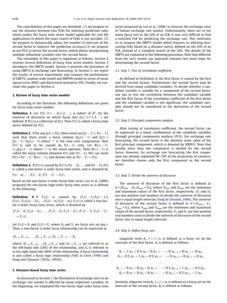
day, three-day, five-day and seven-day exchange rate forecasting,respectively. As shown in Table 9, DBFTS has the smallest MSEand largest DS among the three models for one-day forecasting. Thisresult is consistent with Fig. 3, in which the line of DBFTS is muchcloser to the line of the actual exchange rate than those of RWand RBFNN are. It also shows that when the exchange rate changesrapidly, RW and RBFNN models produce many spikes which aredetrimental to the prediction accuracy. Fortunately, this phenome-non does not exist in DBFTS. To summarize, the experimental re-sults show the following: (1) the MSE of DBFTS is smaller thanthose of RW and RBFNN models; (2) the DS of DBFTS is close to60%, which is much larger than those of RW and RBFNN models.

Fig. 5. Time series of five-day forecasting.

Fig. 6. Time series of seven-day forecasting.

Fig. 4. Time series of three-day forecasting.

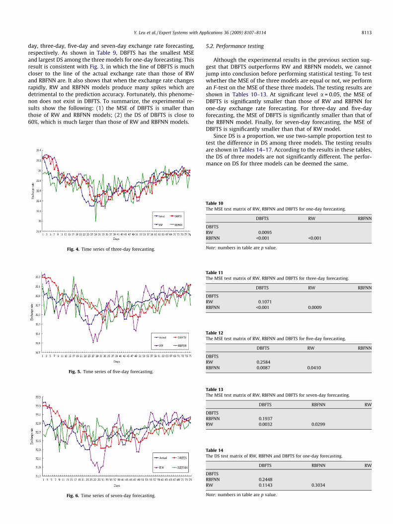
5.2. Performance testing

Although the experimental results in the previous section sug-gest that DBFTS outperforms RW and RBFNN models, we cannotjump into conclusion before performing statistical testing. To testwhether the MSE of the three models are equal or not, we performan F-test on the MSE of these three models. The testing results areshown in Tables 10–13. At significant level a = 0.05, the MSE ofDBFTS is significantly smaller than those of RW and RBFNN forone-day exchange rate forecasting. For three-day and five-dayforecasting, the MSE of DBFTS is significantly smaller than that ofthe RBFNN model. Finally, for seven-day forecasting, the MSE ofDBFTS is significantly smaller than that of RW model.

Since DS is a proportion, we use two-sample proportion test totest the difference in DS among three models. The testing resultsare shown in Tables 14–17. According to the results in these tables,the DS of three models are not significantly different. The perfor-mance on DS for three models can be deemed the same.

Table 10The MSE test matrix of RW, RBFNN and DBFTS for one-day forecasting.

DBFTS RW RBFNN

DBFTSRW 0.0095RBFNN <0.001 <0.001


Table 11The MSE test matrix of RW, RBFNN and DBFTS for three-day forecasting.

DBFTS RW RBFNN

DBFTSRW 0.1071RBFNN <0.001 0.0009

Table 12The MSE test matrix of RW, RBFNN and DBFTS for five-day forecasting.

DBFTS RW RBFNN

DBFTSRW 0.2584RBFNN 0.0087 0.0410

Table 13The MSE test matrix of RW, RBFNN and DBFTS for seven-day forecasting.

DBFTS RBFNN RW

DBFTSRBFNN 0.1937RW 0.0032 0.0299

Table 14The DS test matrix of RW, RBFNN and DBFTS for one-day forecasting.

DBFTS RBFNN RW

DBFTSRBFNN 0.2448RW 0.1143 0.3034


Table 15The DS test matrix of RW, RBFNN and DBFTS for three-day forecasting.

DBFTS RW RBFNN

DBFTSRW 0.5RBFNN 0.2570 0.2570

Table 16The DS test matrix of RW, RBFNN and DBFTS for five-day forecasting.

DBFTS RBFNN RW

DBFTSRBFNN 0.2512RW 0.2012 0.5662

Table 17The DS test matrix of RW, RBFNN and DBFTS for seven-day forecasting.

DBFTS RBFNN RW

DBFTSRBFNN 0.2448RW 0.1143 0.3034


6. Conclusion

Fuzzy time series has been successfully applied in many appli-cations. To overcome the difficulty in finding matching rules forforecasting in the fuzzy time series model, we have proposed touse the Euclidean distance between two fuzzy logic relationshipsas a metric for selecting matching rules. This extension makesthe fuzzy time series model more applicable for applications forwhich complete matching of the fuzzy logic relationships is notpossible. To show the feasibility of the proposed model, we applied

it on forecasting the exchange rate of NTD/USD. Through experi-ments, we showed that the proposed model outperformed the ran-dom walk model and the artificial neural network model in termsof mean square error.

References

Benjamin, M. T. (2006). The dynamic relationship between stock prices andexchange rates: Evidence for Brazil. International Journal of Theoretical andApplied Finance, 9(8), 1377–1396.

Cao, D. Z., Pang, S. L., & Bai, Y. H. (2005). Forecasting exchange rate using supportvector machines. In Proceedings of the 4th international conference on machinelearning and cybernetics, Guangzhou, 18–21 August 2005.

Chen, S. M. (1996). Forecasting enrollments based on fuzzy time series. Fuzzy Setsand Systems, 81(3), 311–319.

Chen, S. M. (2002). Forecasting enrollments based on high-order fuzzy time series.Cybernetics and Systems, 33(1), 1–16.

Cheng, C. H., Chen, T. L., Teoh, H. J., & Chiang, C. H. (2008). Fuzzy time-series basedon adaptive expectation model for TAIEX forecasting. Expert Systems withApplications, 34, 1126–1132.

Lee, L. W., Wang, L. H., Chen, S. M., & Leu, Y. H. (2006). Handling forecastingproblems based on two-factors high-order fuzzy time series. IEEE Transactionson Fuzzy Systems, 14(3), 468–477.

Meese, R. A., & Rogoff, K. (1983). Empirical exchange rate models of the seventies:Do they fit out of sample? Journal of International Economics, 14, 3–24.

Nieh, C. C., & Lee, C. F. (2001). Dynamic relationship between stock prices andexchange rates for G-7 countries. Quarterly Review of Economics and Finance,41(4), 477–490.

Panda, C., & Narasimhan, V. (2007). Forecasting exchange rate better with artificialneural network. Journal of Policy Modeling, 29, 227–236.

R Project for Statistical Computing. The official website of the R Project forStatistical Computing. <http://www.r-project.org/>.

Shin, T., & Han, I. (2000). Optimal signal multi-resolution by genetic algorithms tosupport artificial neural networks for exchange-rate forecasting. Expert Systemswith Applications, 18, 257–269.

Song, Q., & Chissom, B. S. (1993a). Fuzzy time series and its models. Fuzzy Sets andSystems, 54(3), 269–277.

Song, Q., & Chissom, B. S. (1993b). Forecasting enrollments with fuzzy time series –Part I. Fuzzy Sets and Systems, 54(1), 1–9.

Song, Q., & Chissom, B. S. (1994). Forecasting enrollments with fuzzy time series –Part II. Fuzzy Sets and Systems, 62(1), 1–8.

Yu, H. K. (2005). Weighted fuzzy time series models for TAIEX forecasting. Physica A,349, 609–624.

http://www.r-project.org

a distance-based fuzzy time series model for exchange rates forecasting

Documents