a direct simulation method for subsonic, microscale gas flows
TRANSCRIPT
Journal of Computational Physics 179, 400–425 (2002)doi:10.1006/jcph.2002.7061
A Direct Simulation Method for Subsonic,Microscale Gas Flows
Quanhua Sun and Iain D. Boyd
Department of Aerospace Engineering, University of Michigan, Ann Arbor, Michigan 48109E-mail: [email protected], [email protected]
Received November 12, 2001; revised March 25, 2002
Microscale gas flows are the subject of increasingly active research due to therapid advances in micro-electro-mechanical systems (MEMS). The rarefied pheno-mena in MEMS gas flows make molecular-based simulations desirable. However, itis necessary to reduce the statistical scatter in particle methods for microscale gasflows. In this paper, the development of an information preservation (IP) method isdescribed. The IP method reduces the statistical scatter by preserving macroscopicinformation of the flow in the particles and the computational cells simulated inthe direct simulation Monte Carlo (DSMC) method. The preserved macroscopic in-formation of particles is updated during collisions and is then modified to includethe pressure field effects excluded in the collisions. An additional energy trans-fer model is proposed to describe the energy flux across an interface, and a colli-sion model is used to redistribute the information after both particle–particle andparticle–surface collisions. To validate the IP method, four different flows are simu-lated and the solutions are compared against DSMC results. The results from the IPmethod generally agree very well with the DSMC results for steady flows and low fre-quency unsteady flows ranging from the near-continuum regime to the free-molecularregime. c© 2002 Elsevier Science (USA)
Key Words: information preservation method; direct simulation Monte Carlomethod; microscale gas flows; subsonic flows; rarefied gas dynamics.
I. INTRODUCTION
Simulation of gas flow around microscale structures is gaining importance due to the rapiddevelopment of micro-electro-mechanical systems (MEMS) [1, 2]. Previous investigations[3–5] have shown that the fluid behavior around MEMS is different from the macroscopiccounterparts. However, experimental study of microscale gas flows is made inherentlydifficult by the small physical dimensions and has been mainly limited to simple structures,such as micro channels and micro nozzles [3, 6]. Numerical modeling is also a challenge
400
0021-9991/02 $35.00c© 2002 Elsevier Science (USA)
All rights reserved.
SIMULATION METHOD FOR MICROSCALE GAS FLOWS 401
because the MEMS components operate in a variety of flow regimes covering the continuum,slip, and transition regimes.
The flow regimes can be characterized by the Knudsen number (Kn, the ratio of gas meanfree path λ to a characteristic microfluidic length L). Typically, the continuum regime is inthe range of Kn ≤ 0.01, the slip regime is 0.01 ≤ Kn ≤ 0.1, and the Knudsen number of thetransition regime is between 0.1 and 10. For air flows in the slip regime, the air in contactwith the body surface may have a nonzero tangential velocity relative to the surface, andtraditional computational fluid dynamic techniques can be used only if a slip wall conditionis adopted instead of the usual nonslip boundary condition. However, for transition flows(λ ∼ L), collisions between molecules and collisions of molecules with the wall have thesame order of probability. In this case, general kinetic models are required to include therarefied phenomena.
The direct simulation Monte Carlo (DSMC) method is one of the most successful par-ticle simulation methods for rarefied gas flows [7, 8]. Several review articles about theDSMC method are available [9–11]. However, the DSMC method cannot effectively reducethe statistical scatter encountered in microscale flows, which gives a very large noise-to-information ratio since the flows usually have low speed and/or small temperature variation.For microscale flows, several particle methods have been proposed [12–15]. Fan and otherresearchers have developed an information preservation (IP) method for low speed rarefiedgas flows [12, 13, 16–18]. The IP method uses the molecular velocities of the DSMC methodas well as physical information that describes the collective behavior of the large number ofmolecules that a simulated particle represents, and additional treatment is used to update thephysical information. Meanwhile, Pan and co-workers proposed a molecular block modelDSMC method based on the relationship between the statistical scatter and the molecularmass [15]. In their method, the reference diameter and number density of the so-called bigmolecule are determined by ensuring that the mean free path and dynamic viscosity of thebig molecule are equal to those of the real constituent molecules. However, both methodshave not been tested for general microscale flows.
In the present paper, the information preservation method for general 2D microscale flowsis developed. The preserved macroscopic information is first solved in a similar way to themicroscopic information in the DSMC method and is then modified to include the pressureeffects. With two proposed models, the IP method is applied to simulate four different flows.The main purpose of this paper is to demonstrate the validity of the proposed implementationof the IP method since previous papers have shown its ability in decreasing the statisticalscatter for particle methods.
II. INFORMATION PRESERVATION METHOD
2.1. Background and Basic Idea
The information preservation method, first proposed by Fan and Shen [12], was used toovercome the problem of statistical scatter in the DSMC method for low-speed, constantdensity flow systems. It achieved great success for several unidirectional transitional gasflows as shown in [13], including Couette flow, Poiseuille flow, and the Rayleigh problem.This method was later developed by Cai et al. in simulating low-speed microchannel flows[16] and investigating the flows around a NACA0012 airfoil [18] by calculating the macro-scopic velocity and solving the density flow field from the continuity equation. However,
402 SUN AND BOYD
the isothermal assumption used in their implementation limits the further applications ofthe method. In this paper, the IP method is developed for general microscale gas flows, andmodels are proposed when necessary.
The basic idea of the IP method is based on the following consideration. It is generallyrequired that each particle simulated in the DSMC method represents an enormous number(108–1025) of real molecules, and the velocity of these particles can be split into two parts
U = V + C, (1)
where U is the particle velocity, V is the mean molecular velocity, and C is the thermalvelocity. In other words, the particle carries the sum of the macroscopic velocity of a gasflow V (V = U ) and the velocity scatter C (C = 0). The information preservation methodaims to preserve and update the macroscopic information of a gas flow, intending to reducethe statistical scatter inherent in particle methods.
In general, the particle carries the sum of the gas macroscopic information and the infor-mation scatter. From this view, we intend to additionally preserve the energy information(represented by temperature T ) in simulated DSMC particles for general gas flows.
2.2. Principle
The general equation for dilute gas flows is the Boltzmann equation
∂
∂t(n f ) + �c · ∂
∂�r (n f ) + �F · ∂
∂ �c (n f ) =∞∫
−∞
4π∫0
n2( f ∗ f ∗1 − f f1)crσ d d�c1, (2)
where f is the velocity distribution function, n is the number density, t is the time, �ris the physical space vector, �c is the velocity space vector, �F is the external force perunit mass, cr is the relative speed between a molecule of class �c and one of class �c1, andσd is the differential cross section for the collision of a molecule of class �c with oneof class �c1 such that their postcollision velocities are �c∗ and �c∗
1, respectively. Due to thecomplexity of this equation, especially the collision term on the right-hand side of theequation, the direct simulation Monte Carlo method is often used to simulate dilute gasflows. The DSMC method does not solve the Boltzmann equation, however, it does providesolutions that are consistent with the Boltzmann equation. It is assumed that the moleculemotion can be decoupled from the molecule collisions and the gas can be representedby a set of tracking particles (representative molecules) for dilute gas flows. The DSMCmethod tracks the particles with their individual location, velocity, and internal energy, andmodels both particle–particle and particle–surface collisions probabilistically. An importantassumption for the IP method is that the particles simulated in the DSMC method can carrythe macroscopic information of the flow field and the macroscopic information is changedduring collisions. Then the key part of the IP method is how to evaluate particle collisionsfor the macroscopic information.
For low-speed, constant density flow systems, Fan and Shen [12] used the followingsimple collision model for the preserved macroscopic velocity
V ′′1 = V ′′
2 = (V ′1 + V ′
2)/2, (3)
SIMULATION METHOD FOR MICROSCALE GAS FLOWS 403
where superscripts ′ and ′′ denote pre- and postcollision, and subscripts 1 and 2 denoteparticles 1 and 2 in the collision pair. However, for general flows, it is quite a challengeto model the effect of particle collisions on all macroscopic information. It is believedthat particle collisions lead to momentum and energy exchange. Hence, it is necessary topreserve the macroscopic velocity and temperature in particles. Further, if we considercontinuum flows, it is clear that the macroscopic velocity and temperature are changed notonly by the momentum and energy exchange but also by the pressure field. Therefore, forthe IP method, two steps are required. One is the collision and movement step where thewhole DSMC algorithm is applied to both the original DSMC variables and the preservedmacroscopic information, and the other is the modification step, which is used to includethe pressure effects. During the modification step, the following equations are solved withthe help of the macroscopic information that is preserved in the computational cells,
∂Vi
∂t= − 1
ρc
∂pc
∂ri(4)
∂
∂t
(Vi · Vi
2+ ξ · R · T
2
)= − 1
ρc
∂
∂ri(Vi,c · pc), (5)
where p is the pressure, ρ is the mass density, R is the specific gas constant, ξ is the numberof internal degrees of freedom of molecules, and the subscript c denotes the macroscopicinformation for the computational cells. Variables ρc and pc are calculated using Eqs. (6)and (7), respectively, and Tc and Vi,c are sampled from the particles within the cell, whichwill be detailed in the implementation section.
∂ρc
∂t= − ∂
∂ri(ρc · Vi,c) (6)
pc = ρc · R · Tc. (7)
2.3. Additional Energy Transfer Model
As can be seen, the IP method is based on the microscopic movement of the particlessimulated in the DSMC method. There is a contradiction between the real flux and the IPrepresentation about the energy flux across an interface (e.g., a surface of a computationalcell). The net energy flux across an interface is zero in stationary equilibrium flows. However,the average translational energy carried by a molecule across an interface is 2kT , whichis different from 3kT/2, the average translational energy of a molecule. Here k is theBoltzmann constant. In equilibrium flows, this difference arises because the translationalenergy flux of the component normal to the interface is twice the flux of the componentin the other directions. For general nonequilibrium flows, the difference here cannot bebalanced. Hence, it is necessary to introduce additional energy flux for the IP method. Inthe literature, several attempts have been made for general flows [20, 21], but the resultsare far from satisfactory. In this paper, an approximate model is proposed as follows.
The current model aims to capture the net energy flux across an interface instead ofrecovering the microscopic energy for every particle. A simple example may illustrate thismodel. A plate separates a gas with one part at temperature T1 and the other at T2. After theplate is removed, some molecules described by T1 will move to the other side. On average,the T1 particles will transfer 3kT1/2 plus an additional kT1/2 to the other side, and vice versa.
404 SUN AND BOYD
Assuming that the number of particles crossing in each direction is equal, then the net energyflux based on the moving particles is 3k(T1 − T2)/2 plus the additional k(T1 − T2)/2. Thisprocess is modeled by assuming that the T1 particles will transfer 3kT1/2 plus an additionalk(T1 − Tref)/2 to the other side, and the T2 particles will transfer 3kT2/2 plus an additionalk(T2 − Tref)/2 to the other side, where Tref is a reference temperature. Therefore, the IPmethod captures the net energy flux across an interface in an average sense.
In the IP method, when a particle crosses an interface, it carries an additional energy that isto be determined in some way, and the particle “borrows” some energy from other particlesto satisfy the conservation of energy. As illustrated in the example, the additional energyis taken as k(T − Tref)/2, where Tref is very close to the preserved temperature T of theparticle. It is clear that part of the additional energy kTref/2 of one particle must be balancedby another particle such that the net flux across an interface can be correctly modeled. Forstationary gas flows, the number of particles crossing in each direction is the same. Hence,the reference temperature can be taken as the temperature on the interface that a particlewill cross, which can be interpolated from the preserved temperatures of two neighboringcells. Then the effect of the additional energy kTref/2 of one particle will be balanced byanother particle that will cross the same interface from the other direction. For steady flowswith small bulk velocity, however, the number of particles crossing in each direction is notthe same, but very close. The additional energy kTref/2 of most of the particles crossing oneinterface can be balanced by other particles crossing the same interface from the other side,and the additional energy kTref/2 of the particles that are not balanced needs to be balancedby another means. Statistically, there is another molecule leaving a computational cell fromone interface when a molecule enters the cell through another interface for steady flows.Therefore, the additional energy kTref/2 of the particles that enter a cell from one interfaceand are not balanced by the above means can be approximately balanced by particles leavingthe cell from other interfaces because the difference of the reference temperatures (the flowtemperatures on different interfaces) is relatively small. Hence, the additional energy transfermodel can model the net energy flux approximately for steady flows. For unsteady flows, themodel can also be a good approximation if the frequency is low or the temperature variation issmall. In the implementation, the IP method preserves an additional variable Ta for particlesto describe the additional energy k(T − Tref)/2 as ξkTa/2. As stated earlier, the additionalenergy is borrowed from other particles, so a new variable Ta,c is preserved for cells torecord the borrowed energy as ξkTa,c/2. At the end of each time step, the borrowed energyis evenly provided by all the particles in the cell to maintain the conservation of energy.
2.4. General Implementation
For subsonic, microscale flows, nonequilibrium between the translational energy andinternal energy is not significant. Hence, only one temperature is used to denote the internalenergy. In our 2D parallel IP code that is based on a parallel optimized DSMC code named“MONACO” [19], velocity components Vx , Vy and temperatures T , Ta are preserved foreach simulated particle. Velocity components Vx,c, Vy,c, temperatures Tc, Ta,c, and densityρc are preserved for each computational cell.
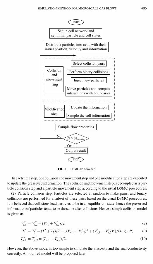
The general implementation of the IP procedures (based on the DSMC procedures) canbe summarized as follows (see also Fig. 1):
(1) Initialization: The information for all the particles and cells is initialized by theambient conditions after the computational domain is set up, while Ta and Ta,c are set to zero.
SIMULATION METHOD FOR MICROSCALE GAS FLOWS 405
start
Set up cell network and set initial particle and cell states
Distribute particles into cells with their initial position, velocity and information
Select collision pairs
Perform binary collisions
Inject new particles
Move particles and compute interactions with boundaries
Update the information
Sample the cell information
Collision and
movement
step
Modificationstep
N > Niteration
Sample flow properties
Output result
stop
No
Yes
FIG. 1. DSMC-IP flowchart.
In each time step, one collision and movement step and one modification step are executedto update the preserved information. The collision and movement step is decoupled as a par-ticle collision step and a particle movement step according to the usual DSMC procedures.
(2) Particle collision step: Particles are selected at random to make pairs, and binarycollisions are performed for a subset of these pairs based on the usual DSMC procedures.It is believed that collisions lead particles to be in an equilibrium state; hence the preservedinformation of particles tends to be the same after collisions. Hence a simple collision modelis given as
V ′′i,1 = V ′′
i,2 = (V ′i,1 + V ′
i,2)/2 (8)
T ′′1 = T ′′
2 = (T ′1 + T ′
2)/2 + (V ′x,1 − V ′
x,2)2 + (V ′
y,1 − V ′y,2)
2�/(4 · ξ · R) (9)
T ′′a,1 = T ′′
a,2 = (T ′a,1 + T ′
a,2)/2. (10)
However, the above model is too simple to simulate the viscosity and thermal conductivitycorrectly. A modified model will be proposed later.
406 SUN AND BOYD
(3) Particle movement step: Particles are moved with the molecular velocity as in theDSMC method. The preserved information of particles may change when particles interactwith interfaces. Possible particle–interface interactions are:
(3a) Particles migrate from one cell to another. When particle j moves from cell kto another cell, momentum and energy transfer occurs, and additional energy transfer isrequired as stated in Section 2.3. The preserved additional energy for the particle and forthe cell are adjusted as
T ′a, j = (Tj − Tref)/ξ (11)
T ′a,c,k = Ta,c,k + Ta, j − T ′
a, j , (12)
where, Tref is the interface temperature interpolated from the preserved cell temperaturesof neighboring cells.
(3b) Particles leave or enter the computational domain. If a particle leaves the com-putational domain, the preserved information of the particle is lost along with the particleitself. As in the DSMC method, new particles may enter into the computational domain, andthese particles are assigned information according to the boundary condition with Ta = 0.
(3c) Particles reflect from a symmetric boundary. When a particle reaches a symmetricboundary, it reflects from the boundary. The normal velocity component is reversed, andthe parallel velocity component remains unchanged.
(3d) Particles reflect from a wall. The preserved information of particles collided witha wall is set in accordance with the collective behavior of a large number of real molecules.Namely, if it is a specular reflection, only the normal velocity component will be reversed.However, if it is a diffuse reflection, the preserved velocity and temperature of the re-flected particles are set to the wall velocity and temperature. Also, the preserved additionaltemperature is changed.
For specular reflection:
T ′a, j = −Ta, j (13)
T ′a,c,k = Ta,c,k + Ta, j − T ′
a, j . (14)
For diffuse reflection:
T ′′a, j = (Tj − Tref)/ξ (15)
T ′a,c,k = Ta,c,k + Ta, j − T ′′
a, j (16)
T ′a, j = (Tw − Tref)/ξ. (17)
Here, T ′′a, j denotes the additional temperature of the particle when it is “absorbed” by the
wall. And Tref =√
Tj · Tw, the constant gas temperature of collisionless flow between twoplates with one at Tj and the other at Tw [23].
After the collisions and movements of particles are considered, the additional energypreserved by the cell k is shared across all Np particles in the cell:
T ′j = Tj + Ta,c,k/Np (18)
T ′a,c,k = 0. (19)
SIMULATION METHOD FOR MICROSCALE GAS FLOWS 407
(4) Modification step: The preserved information of particles is modified by the pressurefield during the modification step. Equations (4) and (5) are solved using a finite volumemethod:
∂Vi
∂t= − 1
ρc
1
A
∮cell
pc · ni dl (20)
∂
∂t
(Vi · Vi
2+ ξ · R · T
2
)= − 1
ρc
1
A
∮cell
(pc · Vi,cni ) dl (21)
V t+�ti − V t
i = −�t
ρc
1
A
∮cell
pc · ni dl (22)
(Vi · Vi
2+ ξ · R · T
2
)t+�t
−(
Vi · Vi
2+ ξ · R · T
2
)t
= −�t
ρc
1
A
∮cell
(pc · Vi,cni ) dl. (23)
In the above equations, A is the area of the cell, dl is the edge element of the cell, and �n isthe unit vector normal to the cell edge. The integrals are integrated over all cell edges. Thecell information on cell edges is linearly interpolated using the information of the neigh-boring cells. To avoid statistical effects due to the number fluctuation of particles in a cellin Eqs. (20) and (21), the density ρc is replaced by the ratio of the real mass of the totalrepresented molecules in the cell to the volume of the cell. For example,
∂Vi, j
∂t= − 1
ρc
1
A
∮cell
pc · ni dl = − 1
NpWpm/Vol
1
A
∮cell
pc · ni dl (24)
or
Np∑j
1
Vol
∂(WpmVi, j )
∂t= − 1
A
∮cell
pc · ni dl, (25)
where subscript j denotes particle j in the cell, and Wp is the number of gas moleculesrepresented by one particle. It is clear that the number fluctuation of particles in a cell doesnot affect the total pressure effects for all the particles in the cell.
(5) Update cell information: After the preserved information of particles is updated, thepreserved information for cells is updated by averaging the information of all Np particlesin the cell.
V ′i,c =
Np∑j=1
(Vi, j
Np
)(26)
T ′c =
Np∑j=1
(Tj + Ta, j
Np
). (27)
The density is updated by Eq. (6). Again, it is solved by a finite volume method:
∂ρc
∂t= − 1
A
∮cell
(ρc · Vi,c · ni ) dl. (28)
408 SUN AND BOYD
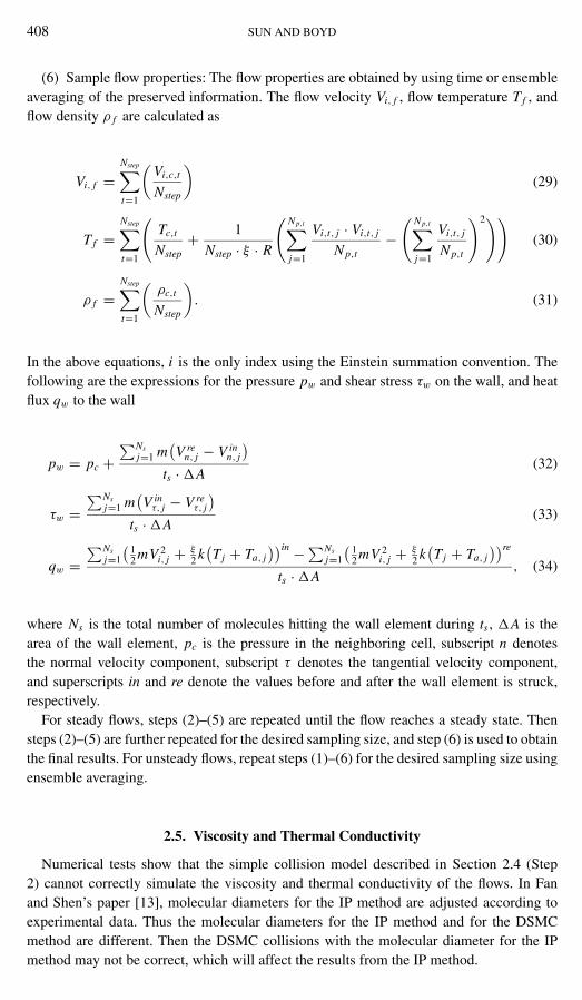
(6) Sample flow properties: The flow properties are obtained by using time or ensembleaveraging of the preserved information. The flow velocity Vi, f , flow temperature T f , andflow density ρ f are calculated as
Vi, f =Nstep∑t=1
(Vi,c,t
Nstep
)(29)
T f =Nstep∑t=1
(Tc,t
Nstep+ 1
Nstep · ξ · R
( Np,t∑j=1
Vi,t, j · Vi,t, j
Np,t−( Np,t∑
j=1
Vi,t, j
Np,t
)2))(30)
ρ f =Nstep∑t=1
(ρc,t
Nstep
). (31)
In the above equations, i is the only index using the Einstein summation convention. Thefollowing are the expressions for the pressure pw and shear stress τw on the wall, and heatflux qw to the wall
pw = pc +∑Ns
j=1 m(V re
n, j − V inn, j
)ts · �A
(32)
τw =∑Ns
j=1 m(V in
τ, j − V reτ, j
)ts · �A
(33)
qw =∑Ns
j=1
(12 mV 2
i, j + ξ
2 k(Tj + Ta, j
))in −∑Nsj=1
(12 mV 2
i, j + ξ
2 k(Tj + Ta, j
))re
ts · �A, (34)
where Ns is the total number of molecules hitting the wall element during ts , �A is thearea of the wall element, pc is the pressure in the neighboring cell, subscript n denotesthe normal velocity component, subscript τ denotes the tangential velocity component,and superscripts in and re denote the values before and after the wall element is struck,respectively.
For steady flows, steps (2)–(5) are repeated until the flow reaches a steady state. Thensteps (2)–(5) are further repeated for the desired sampling size, and step (6) is used to obtainthe final results. For unsteady flows, repeat steps (1)–(6) for the desired sampling size usingensemble averaging.
2.5. Viscosity and Thermal Conductivity
Numerical tests show that the simple collision model described in Section 2.4 (Step2) cannot correctly simulate the viscosity and thermal conductivity of the flows. In Fanand Shen’s paper [13], molecular diameters for the IP method are adjusted according toexperimental data. Thus the molecular diameters for the IP method and for the DSMCmethod are different. Then the DSMC collisions with the molecular diameter for the IPmethod may not be correct, which will affect the results from the IP method.
SIMULATION METHOD FOR MICROSCALE GAS FLOWS 409
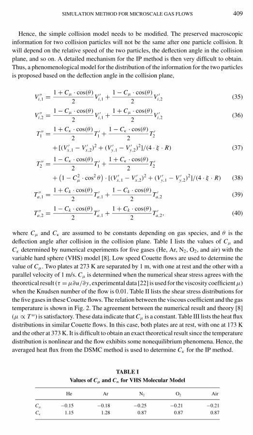
Hence, the simple collision model needs to be modified. The preserved macroscopicinformation for two collision particles will not be the same after one particle collision. Itwill depend on the relative speed of the two particles, the deflection angle in the collisionplane, and so on. A detailed mechanism for the IP method is then very difficult to obtain.Thus, a phenomenological model for the distribution of the information for the two particlesis proposed based on the deflection angle in the collision plane,
V ′′i,1 = 1 + Cµ · cos(θ)
2V ′
i,1 + 1 − Cµ · cos(θ)
2V ′
i,2 (35)
V ′′i,2 = 1 − Cµ · cos(θ)
2V ′
i,1 + 1 + Cµ · cos(θ)
2V ′
i,2 (36)
T ′′1 = 1 + Cκ · cos(θ)
2T ′
1 + 1 − Cκ · cos(θ)
2T ′
2
+ [(V ′x,1 − V ′
x,2)2 + (V ′
y,1 − V ′y,2)
2]/(4 · ξ · R) (37)
T ′′2 = 1 − Cκ · cos(θ)
2T ′
1 + 1 + Cκ · cos(θ)
2T ′
2
+ (1 − C2µ · cos2 θ
) · [(V ′x,1 − V ′
x,2)2 + (V ′
y,1 − V ′y,2)
2]/(4 · ξ · R) (38)
T ′′a,1 = 1 + Ck · cos(θ)
2T ′
a,1 + 1 − Ck · cos(θ)
2T ′
a,2 (39)
T ′′a,2 = 1 − Ck · cos(θ)
2T ′
a,1 + 1 + Ck · cos(θ)
2T ′
a,2, (40)
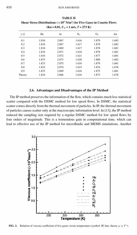
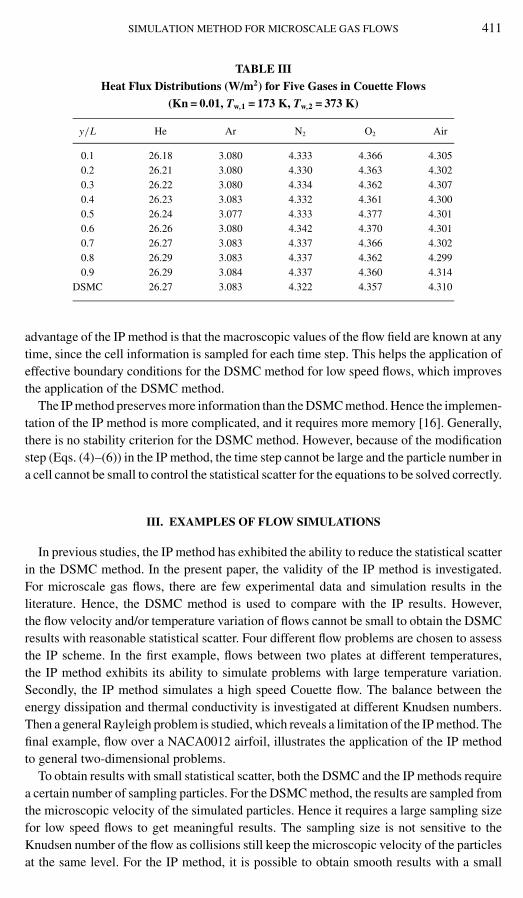
where Cµ and Cκ are assumed to be constants depending on gas species, and θ is thedeflection angle after collision in the collision plane. Table I lists the values of Cµ andCκ determined by numerical experiments for five gases (He, Ar, N2, O2, and air) with thevariable hard sphere (VHS) model [8]. Low speed Couette flows are used to determine thevalue of Cµ. Two plates at 273 K are separated by 1 m, with one at rest and the other with aparallel velocity of 1 m/s. Cµ is determined when the numerical shear stress agrees with thetheoretical result (τ = µ∂u/∂y, experimental data [22] is used for the viscosity coefficient µ)when the Knudsen number of the flow is 0.01. Table II lists the shear stress distributions forthe five gases in these Couette flows. The relation between the viscous coefficient and the gastemperature is shown in Fig. 2. The agreement between the numerical result and theory [8](µ ∝ T ω) is satisfactory. These data indicate that Cµ is a constant. Table III lists the heat fluxdistributions in similar Couette flows. In this case, both plates are at rest, with one at 173 Kand the other at 373 K. It is difficult to obtain an exact theoretical result since the temperaturedistribution is nonlinear and the flow exhibits some nonequilibrium phenomena. Hence, theaveraged heat flux from the DSMC method is used to determine Cκ for the IP method.
TABLE I
Values of Cµ and Cκ for VHS Molecular Model
He Ar N2 O2 Air
Cµ −0.15 −0.18 −0.25 −0.21 −0.21Cκ 1.15 1.28 0.87 0.87 0.87
410 SUN AND BOYD
TABLE II
Shear Stress Distributions (×105 N/m2) for Five Gases in Couette Flows
(Kn = 0.01, Uw = 1 m/s, T = 273 K)
y/L He Ar N2 O2 Air
0.1 1.834 2.067 1.616 1.879 1.6830.2 1.834 2.067 1.617 1.878 1.6820.3 1.834 2.069 1.617 1.878 1.6810.4 1.834 2.071 1.618 1.878 1.6810.5 1.834 2.072 1.621 1.877 1.6810.6 1.833 2.073 1.620 1.880 1.6820.7 1.833 2.075 1.618 1.879 1.6810.8 1.832 2.074 1.615 1.876 1.6780.9 1.833 2.069 1.616 1.875 1.681
Theory 1.824 2.066 1.616 1.873 1.678
2.6. Advantages and Disadvantages of the IP Method
The IP method preserves the information of the flow, which contains much less statisticalscatter compared with the DSMC method for low speed flows. In DSMC, the statisticalscatter comes directly from the thermal movement of particles. In IP, the thermal movementof particles causes scatter only at the macroscopic information level. In [13], the IP methodreduced the sampling size required by a regular DSMC method for low speed flows byfour orders of magnitude. This is a tremendous gain in computational time, which canlead to effective use of the IP method for microfluidic and MEMS simulations. Another
FIG. 2. Relation of viscous coefficient of five gases versus temperature (symbol: IP, line: theory µ ∝ T ω).
SIMULATION METHOD FOR MICROSCALE GAS FLOWS 411
TABLE III
Heat Flux Distributions (W/m2) for Five Gases in Couette Flows
(Kn = 0.01, Tw,1 = 173 K, Tw,2 = 373 K)
y/L He Ar N2 O2 Air
0.1 26.18 3.080 4.333 4.366 4.3050.2 26.21 3.080 4.330 4.363 4.3020.3 26.22 3.080 4.334 4.362 4.3070.4 26.23 3.083 4.332 4.361 4.3000.5 26.24 3.077 4.333 4.377 4.3010.6 26.26 3.080 4.342 4.370 4.3010.7 26.27 3.083 4.337 4.366 4.3020.8 26.29 3.083 4.337 4.362 4.2990.9 26.29 3.084 4.337 4.360 4.314
DSMC 26.27 3.083 4.322 4.357 4.310
advantage of the IP method is that the macroscopic values of the flow field are known at anytime, since the cell information is sampled for each time step. This helps the application ofeffective boundary conditions for the DSMC method for low speed flows, which improvesthe application of the DSMC method.
The IP method preserves more information than the DSMC method. Hence the implemen-tation of the IP method is more complicated, and it requires more memory [16]. Generally,there is no stability criterion for the DSMC method. However, because of the modificationstep (Eqs. (4)–(6)) in the IP method, the time step cannot be large and the particle number ina cell cannot be small to control the statistical scatter for the equations to be solved correctly.
III. EXAMPLES OF FLOW SIMULATIONS
In previous studies, the IP method has exhibited the ability to reduce the statistical scatterin the DSMC method. In the present paper, the validity of the IP method is investigated.For microscale gas flows, there are few experimental data and simulation results in theliterature. Hence, the DSMC method is used to compare with the IP results. However,the flow velocity and/or temperature variation of flows cannot be small to obtain the DSMCresults with reasonable statistical scatter. Four different flow problems are chosen to assessthe IP scheme. In the first example, flows between two plates at different temperatures,the IP method exhibits its ability to simulate problems with large temperature variation.Secondly, the IP method simulates a high speed Couette flow. The balance between theenergy dissipation and thermal conductivity is investigated at different Knudsen numbers.Then a general Rayleigh problem is studied, which reveals a limitation of the IP method. Thefinal example, flow over a NACA0012 airfoil, illustrates the application of the IP methodto general two-dimensional problems.
To obtain results with small statistical scatter, both the DSMC and the IP methods requirea certain number of sampling particles. For the DSMC method, the results are sampled fromthe microscopic velocity of the simulated particles. Hence it requires a large sampling sizefor low speed flows to get meaningful results. The sampling size is not sensitive to theKnudsen number of the flow as collisions still keep the microscopic velocity of the particlesat the same level. For the IP method, it is possible to obtain smooth results with a small

412 SUN AND BOYD
sampling size because each particle carries the macroscopic information. However, it isvery sensitive to the Knudsen number of the flow because particle collisions smooth thepreserved macroscopic information of the particles. Therefore, the IP method needs veryfew time steps to obtain meaningful results for low speed gas flows with small Knudsennumber. In the first three examples, the computational domain is divided into 200 cells.To get meaningful results, the DSMC method needs about 100,000 particles per cell. Forthe same level of results, the IP method only needs about 1000 particles per cell for flowswith Kn = 0.01 and 10,000 particles per cell for flows with Kn = 100. For the results givenbelow, a much larger sample size (20,000,000 particles per cell for examples 1 and 2, and5,000,000 particles per cell for example 3) is used for both methods because it is better touse good smooth results to validate the method and because a single code is used whereboth results are obtained at the same time.
3.1. Flows between Two Plates at Different Temperatures
The simulation of energy transport is a difficult part in the IP method. Rarefied gas flowbetween two plates at different temperatures is one of the most fundamental problems inrarefied gas dynamics, which can test the energy transport in the IP method. In Fig. 3, twoplates at rest are separated by 1 m, with one at 173 K and the other at 373 K. The density ofthe argon gas is selected such that the Knudsen number of the flows at 273 K ranges from0.01 to 100.
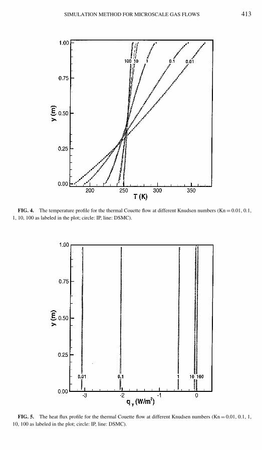
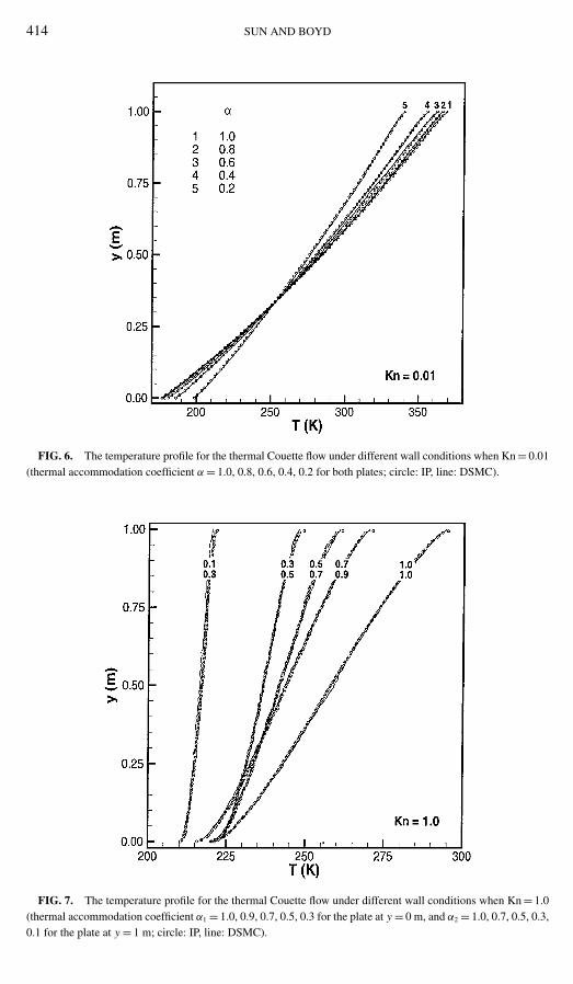
Figure 4 shows the temperature profiles at different Knudsen numbers for the IP methodand the DSMC method when the thermal accommodation coefficient is 1.0. At the Knudsennumbers of 0.01, 0.1, 1.0, and 100, excellent agreement is obtained between the IP and theDSMC results. The difference between the results from two methods when the Knudsennumber is 10, however, is relatively small for such a strongly nonequilibrium flow. Figure 5shows the heat flux for the IP method and the DSMC method. Again, excellent agreement isobtained. The IP method is also examined for different wall conditions when the Knudsennumber is 0.01 and 1.0. When the Knudsen number is 0.01, the thermal accommodationcoefficient for both plates is set as 1.0, 0.8, 0.6, 0.4, and 0.2, respectively. For the Kn = 1.0case, several combinations of the thermal accommodation coefficient of the plates are usedto further check the effects of the wall condition. As can be seen from Figs. 6 and 7, theagreement between the IP results and the DSMC results is also very good.
3.2. High Speed Couette Flow
It is critical that the viscosity and thermal conductivity can be simulated correctly bythe IP method. A good example for this kind of verification is a high speed Couette flow.
y = 0 m
y = 1 m
x
y
plate 2: α2, T2=373K , Vx,2 = 0
plate 1: α1, T1 = 173K, Vx,1 = 0
argon gas
FIG. 3. Schematic diagram for the thermal Couette flow.
SIMULATION METHOD FOR MICROSCALE GAS FLOWS 413
FIG. 4. The temperature profile for the thermal Couette flow at different Knudsen numbers (Kn = 0.01, 0.1,1, 10, 100 as labeled in the plot; circle: IP, line: DSMC).
FIG. 5. The heat flux profile for the thermal Couette flow at different Knudsen numbers (Kn = 0.01, 0.1, 1,10, 100 as labeled in the plot; circle: IP, line: DSMC).
414 SUN AND BOYD
FIG. 6. The temperature profile for the thermal Couette flow under different wall conditions when Kn = 0.01(thermal accommodation coefficient α = 1.0, 0.8, 0.6, 0.4, 0.2 for both plates; circle: IP, line: DSMC).
FIG. 7. The temperature profile for the thermal Couette flow under different wall conditions when Kn = 1.0(thermal accommodation coefficient α1 = 1.0, 0.9, 0.7, 0.5, 0.3 for the plate at y = 0 m, and α2 = 1.0, 0.7, 0.5, 0.3,0.1 for the plate at y = 1 m; circle: IP, line: DSMC).
SIMULATION METHOD FOR MICROSCALE GAS FLOWS 415
y = 0 m
y = 1 m
x
y
plate 2: α2 = 1.0, T2 = 273K, Vx,2 = 300 m/s
plate 1: α1 = 1.0, T1 = 273K, Vx,1 = 0
argon gas
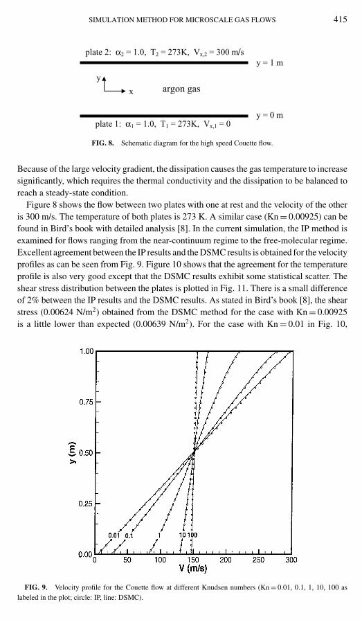
FIG. 8. Schematic diagram for the high speed Couette flow.
Because of the large velocity gradient, the dissipation causes the gas temperature to increasesignificantly, which requires the thermal conductivity and the dissipation to be balanced toreach a steady-state condition.
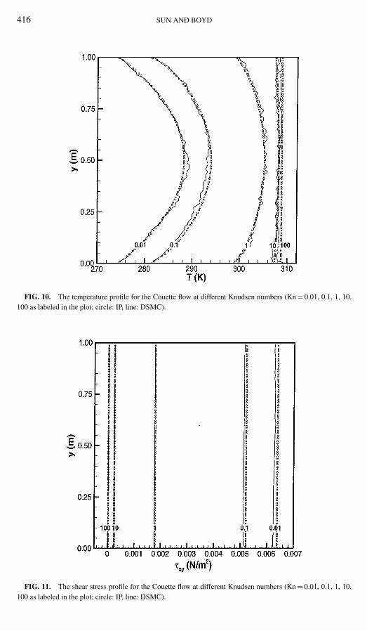
Figure 8 shows the flow between two plates with one at rest and the velocity of the otheris 300 m/s. The temperature of both plates is 273 K. A similar case (Kn = 0.00925) can befound in Bird’s book with detailed analysis [8]. In the current simulation, the IP method isexamined for flows ranging from the near-continuum regime to the free-molecular regime.Excellent agreement between the IP results and the DSMC results is obtained for the velocityprofiles as can be seen from Fig. 9. Figure 10 shows that the agreement for the temperatureprofile is also very good except that the DSMC results exhibit some statistical scatter. Theshear stress distribution between the plates is plotted in Fig. 11. There is a small differenceof 2% between the IP results and the DSMC results. As stated in Bird’s book [8], the shearstress (0.00624 N/m2) obtained from the DSMC method for the case with Kn = 0.00925is a little lower than expected (0.00639 N/m2). For the case with Kn = 0.01 in Fig. 10,
FIG. 9. Velocity profile for the Couette flow at different Knudsen numbers (Kn = 0.01, 0.1, 1, 10, 100 aslabeled in the plot; circle: IP, line: DSMC).
416 SUN AND BOYD
FIG. 10. The temperature profile for the Couette flow at different Knudsen numbers (Kn = 0.01, 0.1, 1, 10,100 as labeled in the plot; circle: IP, line: DSMC).
FIG. 11. The shear stress profile for the Couette flow at different Knudsen numbers (Kn = 0.01, 0.1, 1, 10,100 as labeled in the plot; circle: IP, line: DSMC).
SIMULATION METHOD FOR MICROSCALE GAS FLOWS 417
compared with the DSMC data (0.00626 N/m2), the IP method predicts an average shearstress of 0.00639 N/m2.
3.3. Rayleigh Flow
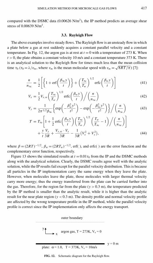
The above examples involve steady flows. The Rayleigh flow is an unsteady flow in whicha plate below a gas at rest suddenly acquires a constant parallel velocity and a constanttemperature. In Fig. 12, the argon gas is at rest at t = 0 with a temperature of 273 K. Whent > 0, the plate obtains a constant velocity 10 m/s and a constant temperature 373 K. Thereis an analytical solution to the Rayleigh flow for times much less than the mean collisiontime τ0 (τ0 = λ/vm , where vm is the mean molecular speed with vm = √
8RT /π ) [7]:
n
n∞= 1
2
[{1 + erf
(β∞y
t
)}+(
T∞Tw
)1/2
erfc
(βw y
t
)](41)
Vx = 1
2Vx,w
(T∞Tw
)1/2
erfc
(βw y
t
)/(n
n∞
)(42)
Vy = 1
2π1/2β∞
{exp
(−β2
w y2
t2
)− exp
(−β2
∞y2
t2
)}/(n
n∞
)(43)
T = T∞
[1 + 1
2erfc
(βw y
t
)(T∞Tw
)1/2( Tw
T∞− 1
)/(n
n∞
)]
+ y
t
Vy
3R+ Vx,w · Vx
3R− 1
3R
(V 2
x + V 2y
), (44)
where β = (2RT )−1/2, βw = (2RTw)−1/2, erf( ), and erfc( ) are the error function and thecomplementary error function, respectively.
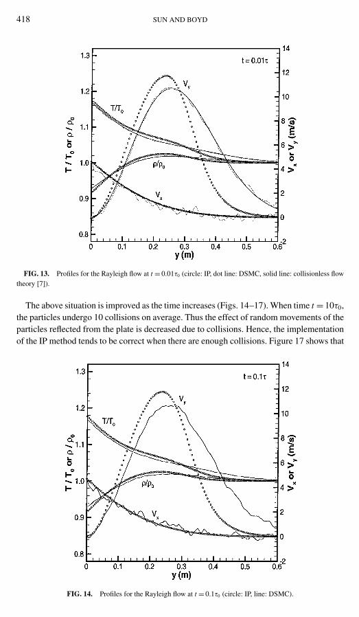
Figure 13 shows the simulated results at t = 0.01τ0 from the IP and the DSMC methodsalong with the analytical solution. Clearly, the DSMC results agree well with the analyticsolution, while the IP results fail except for the parallel velocity distribution. This is becauseall particles in the IP implementation carry the same energy when they leave the plate.However, when molecules leave the plate, those molecules with larger thermal velocitycarry more energy; thus the energy transferred from the plate can be carried further intothe gas. Therefore, for the region far from the plate (y > 0.3 m), the temperature predictedby the IP method is smaller than the analytic result, while it is higher than the analyticresult for the near plate region (y < 0.3 m). The density profile and normal velocity profileare affected by the wrong temperature profile in the IP method, while the parallel velocityprofile is correct since the IP implementation only affects the energy transport.
y = 0 m
outer boundary
x
y
plate: α = 1.0, T = 373K, Vx = 10m/s
argon gas, T = 273K, Vx = 0
FIG. 12. Schematic diagram for the Rayleigh flow.
418 SUN AND BOYD
FIG. 13. Profiles for the Rayleigh flow at t = 0.01τ0 (circle: IP, dot line: DSMC, solid line: collisionless flowtheory [7]).
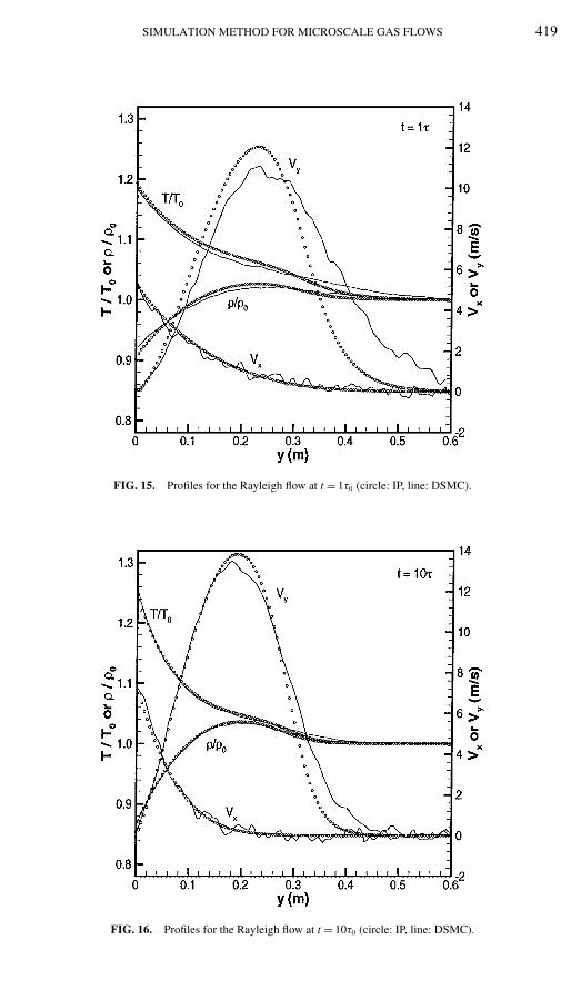
The above situation is improved as the time increases (Figs. 14–17). When time t = 10τ0,the particles undergo 10 collisions on average. Thus the effect of random movements of theparticles reflected from the plate is decreased due to collisions. Hence, the implementationof the IP method tends to be correct when there are enough collisions. Figure 17 shows that
FIG. 14. Profiles for the Rayleigh flow at t = 0.1τ0 (circle: IP, line: DSMC).
SIMULATION METHOD FOR MICROSCALE GAS FLOWS 419
FIG. 15. Profiles for the Rayleigh flow at t = 1τ0 (circle: IP, line: DSMC).
FIG. 16. Profiles for the Rayleigh flow at t = 10τ0 (circle: IP, line: DSMC).
420 SUN AND BOYD
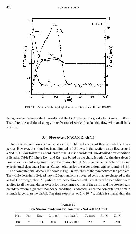
FIG. 17. Profiles for the Rayleigh flow at t = 100τ0 (circle: IP, line: DSMC).
the agreement between the IP results and the DSMC results is good when time t = 100τ0.Therefore, the additional energy transfer model works fine for this flow with small bulkvelocity.
3.4. Flow over a NACA0012 Airfoil
One-dimensional flows are selected as test problems because of their well-defined pro-perties. However, the IP method is not limited to 1D flows. In this section, an air flow arounda NACA0012 airfoil with a chord length of 0.04 m is considered. The detailed flow conditionis listed in Table IV, where Re∞ and Kn∞ are based on the chord length. Again, the selectedflow velocity is not very small such that reasonable DSMC results can be obtained. Someexperimental data and a Navier–Stokes solution for these conditions can be found in [18].
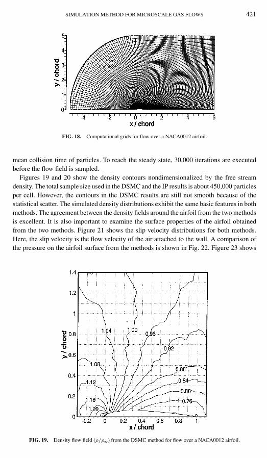
The computational domain is shown in Fig. 18, which uses the symmetry of the problem.The whole domain is divided into 9120 nonuniform structured cells that are clustered to theairfoil. On average, about 50 particles are located in each cell. Free stream flow conditions areapplied to all the boundaries except for the symmetric line of the airfoil and the downstreamboundary where a gradient boundary condition is adopted, since the computation domainis much larger than the airfoil. The time step is set to 5 × 10⁻⁸ s, which is smaller than the
TABLE IV
Free Stream Conditions for Flow over a NACA0012 Airfoil
Ma∞ Re∞ Kn∞ Lchord (m) ρ∞ (kg/m3) U∞ (m/s) T∞ (K) Tw (K)
0.8 73 0.014 0.04 1.116 × 10⁻⁴ 257 257 290
SIMULATION METHOD FOR MICROSCALE GAS FLOWS 421
FIG. 18. Computational grids for flow over a NACA0012 airfoil.
mean collision time of particles. To reach the steady state, 30,000 iterations are executedbefore the flow field is sampled.
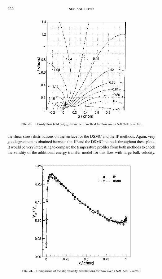
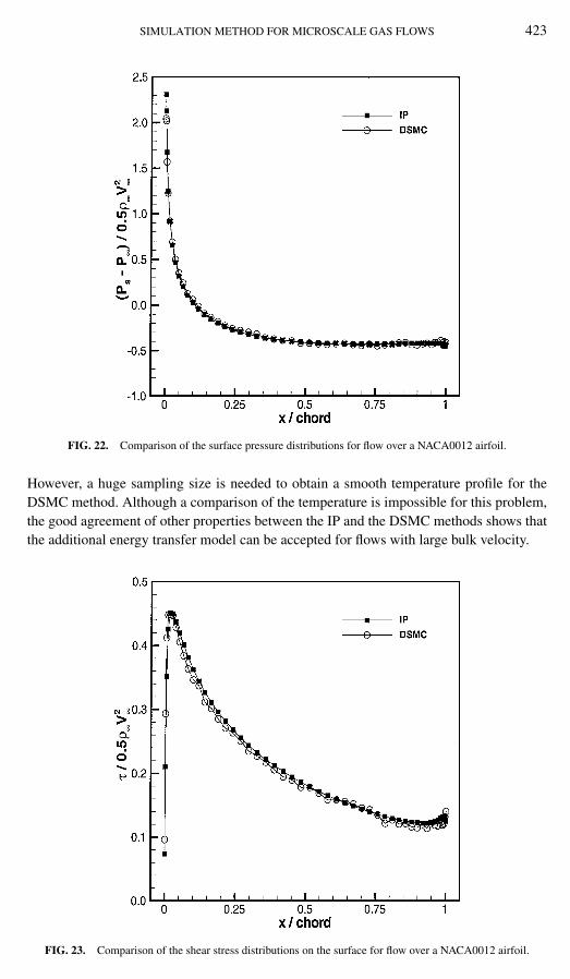
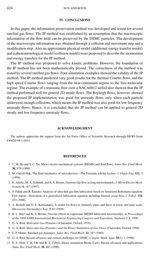
Figures 19 and 20 show the density contours nondimensionalized by the free streamdensity. The total sample size used in the DSMC and the IP results is about 450,000 particlesper cell. However, the contours in the DSMC results are still not smooth because of thestatistical scatter. The simulated density distributions exhibit the same basic features in bothmethods. The agreement between the density fields around the airfoil from the two methodsis excellent. It is also important to examine the surface properties of the airfoil obtainedfrom the two methods. Figure 21 shows the slip velocity distributions for both methods.Here, the slip velocity is the flow velocity of the air attached to the wall. A comparison ofthe pressure on the airfoil surface from the methods is shown in Fig. 22. Figure 23 shows
FIG. 19. Density flow field (ρ/ρ∞) from the DSMC method for flow over a NACA0012 airfoil.
422 SUN AND BOYD
FIG. 20. Density flow field (ρ/ρ∞) from the IP method for flow over a NACA0012 airfoil.
the shear stress distributions on the surface for the DSMC and the IP methods. Again, verygood agreement is obtained between the IP and the DSMC methods throughout these plots.It would be very interesting to compare the temperature profiles from both methods to checkthe validity of the additional energy transfer model for this flow with large bulk velocity.
FIG. 21. Comparison of the slip velocity distributions for flow over a NACA0012 airfoil.
SIMULATION METHOD FOR MICROSCALE GAS FLOWS 423
FIG. 22. Comparison of the surface pressure distributions for flow over a NACA0012 airfoil.
However, a huge sampling size is needed to obtain a smooth temperature profile for theDSMC method. Although a comparison of the temperature is impossible for this problem,the good agreement of other properties between the IP and the DSMC methods shows thatthe additional energy transfer model can be accepted for flows with large bulk velocity.
FIG. 23. Comparison of the shear stress distributions on the surface for flow over a NACA0012 airfoil.
424 SUN AND BOYD
IV. CONCLUSIONS
In this paper, the information preservation method was developed and tested for severalrarefied gas flows. The IP method was established by an assumption that the macroscopicinformation of the flow field can be preserved by the DSMC particles. The developmentof the macroscopic information was obtained through a collision and movement step and amodification step. Also an approximate physical model (additional energy transfer model)and a phenomenological model (collision model) were proposed to describe the momentumand energy transfers for the IP method.
The IP method was proposed to solve kinetic problems. However, the foundation ofthe IP method has not been mathematically proved. The correctness of the method wastested by several rarefied gas flows. Four simulation examples showed the validity of the IPmethod. The IP method predicted very good results for the thermal Couette flows and thehigh speed Couette flows ranging from the near-continuum regime to the free-molecularregime. The example of a transonic flow over a NACA0012 airfoil also showed that the IPmethod performed well for general 2D steady flows. The Rayleigh flows, however, showedthe proposed IP implementation was good for unsteady flows only when each particleunderwent enough collisions, which means the IP method was also good for low frequencyunsteady flows. Hence, it is concluded that the IP method can be applied to general 2Dsteady and low frequency unsteady flows.
ACKNOWLEDGMENT
The authors appreciate the support from the Air Force Office of Scientific Research through MURI GrantF49620-98-1-0433.
REFERENCES
1. C. M. Ho and Y. C. Tai, Micro-electro-mechanical-systems (MEMS) and fluid flows, Annu. Rev. Fluid Mech.30, 579 (1998).
2. M. Gad-el-Hak, The fluid mechanics of microdevices—The Freeman scholar lecture, J. Fluids Eng. 121, 5(1999).
3. E. Arkilic, M. A. Schmidt, and K. S. Breuer, Gaseous slip flow in long microchannels, J. Micro Electro Mech.Systems 6, 167 (1997).
4. S. Fukui and R. Kaneko, Analysis of ultra thin gas film lubrication based on linearized Boltzmann equation:First report—Derivation of a generalized lubrication equation including thermal creep flow, J. Tribol. 110,253 (1988).
5. A. Beskok and G. E. Karniadakis, A model for flows in channels, pipes and ducts at micro and nano scale,Microscale Thermophys. Eng. 3, 43 (1999).
6. R. L. Bayt and K. S. Breuer, Viscous effects in supersonic MEMS-fabricated micronozzles, in Proceedingsof the 1998 ASME International Mechanical Engineering Congress and Exposition, Anaheim, CA, 1998.
7. G. A. Bird, Molecular Gas Dynamics (Clarendon, Oxford, 1976).
8. G. A. Bird, Molecular Gas Dynamics and the Direct Simulation of Gas Flows (Clarendon, Oxford, 1994).
9. E. P. Muntz, Rarefied gas dynamics, Annu. Rev. Fluid Mech. 21, 387 (1989).
10. G. A. Bird, Recent advances and current challenges for DSMC, Comput. Math. Appl. 35(1), 1 (1998).
11. E. S. Oran, C. K. Oh, and B. Z. Cybyk, Direct simulation Monte Carlo: Recent advances and applications,Annu. Rev. Fluid Mech. 30, 403 (1998).
SIMULATION METHOD FOR MICROSCALE GAS FLOWS 425
12. J. Fan and C. Shen, Statistical simulation of low-speed unidirectional flows in transition regime, in RarefiedGas Dynamics, edited by R. Brun et al. (Cepadus-Editions, Toulouse, 1999), Vol. 2, p. 245.
13. J. Fan and C. Shen, Statistical simulation of low-speed rarefied gas flows, J. Comput. Phys. 167, 393 (2001).
14. L. S. Pan, G. R. Liu, B. C. Khoo, and B. Song, Modified direct simulation Monte Carlo method for low-speedmicroflows, J. Micromech. Microeng. 10(1), 21 (2000).
15. L. S. Pan, T. Y. Ng, D. Xu, and K. Y. Lam, Molecular block model direct simulation Monte Carlo method forlow velocity microgas flows, J. Micromech. Microeng. 11, 181 (2001).
16. C. Cai, I. D. Boyd, J. Fan, and G. V. Candler, Direct simulation methods for low-speed microchannel flows,J. Thermophys. Heat Transfer 14(3), 368 (2000).
17. I. D. Boyd and Q. Sun, Particle simulation of micro-scale gas flows, AIAA-01-0876 (Reno, 2001).
18. J. Fan, I. D. Boyd, C. P. Cai, K. Hennighausen, and G. V. Candler, Computation of rarefied flows around aNACA 0012 airfoil, AIAA J. 39(4), 618 (2001).
19. S. Dietrich and I. D. Boyd, Scalar and parallel optimized implementation of the direct simulation Monte Carlomethod, J. Comput. Phys. 126, 328 (1996).
20. C. Shen, J. Z. Jiang, and J. Fan, Information preservation method for the case of temperature variation, inRarefied Gas Dynamics, edited by T. J. Bartel and M. A. Gallis (American Institute of Physics, Melville,2001), p. 185.
21. Q. Sun, I. D. Boyd, and J. Fan, Development of an information preservation method for subsonic, micro-scalegas flows, in Rarefied Gas Dynamics, edited by T. J. Bartel and M. A. Gallis (American Institute of Physics,Melville, 2001), p. 547.
22. S. Chapman and T. G. Cowling, The Mathematical Theory of Non-Uniform Gases, 3rd ed. (Cambridge Univ.Press, Cambridge, UK, 1970).
23. T. I. Gombosi, Gaskinetic Theory (Cambridge Univ. Press, Cambridge, UK, 1994).