a differential approach to graphical...
TRANSCRIPT
A Differential Approach to GraphicalInteraction
Michael L. Gleicher
November 18, 1994CMU-CS-94-217
School of Computer ScienceCarnegie Mellon University
5000 Forbes AvenuePittsburgh, PA 15213-3891
Submitted in partial fulfillment of the requirementsfor the degree of Doctor of Philosophy.
Thesis Committee:Andrew Witkin, Chair
Paul HeckbertBrad Myers
Robert Sproull, Sun Microsystems
c 1994 by Michael L. Gleicher
This research was supported in part by Apple Computer, an equipment grant from Silicon GraphicsInc., and a fellowship from the Schlumberger Foundation. The views and conclusions contained in thisdocument are those of the author and should not be interpretted as representing the official policies, eitherexpressed or implied, of these companies.

Keywords: Constraints, Direct Manipulation, Interaction Techniques, User Inter-face Toolkits

Abstract
Direct manipulation has become the preferred interface forcontrolling graphical ob-jects. Despite its success, the ad hoc manner with which suchinterfaces have beendesigned and implemented restricts the types of interactive controls. This dissertationpresents a new approach that provides a systematic method for implementing flexible,combinable interactive controls. Thisdifferential approachto graphical interactionuses constrained optimization to couple user controls to graphical objects in a mannerthat permits a variety of controls to be freely combined. Thedifferential approach pro-vides a new set of abstractions that enable new types of interaction techniques and newways of modularizing applications.
The differential approach views graphical object manipulation as an equation solv-ing problem: Given the desired values for the user specified controls, find a configura-tion of the graphical objects that meet these constraints. To solve these equations in asufficiently general manner, the differential approach controls the motion of the objectsover time. At any instant in time, controls specify desired rates of change that form lin-ear constraints on the time derivatives of the parameters. An optimization objectiveselects a particular value when these constraints do not determine a unique solution.The differential approach solves these constrained optimization problems to computethe derivatives of the parameters. An ordinary differential equation solver uses theserates to compute object motions.
This thesis addresses the issues in using numerical techniques to provide interac-tive control of graphical objects. Techniques are presented to solve the constrainedoptimization problems efficiently and to dynamically defineequations in response tosystem events. The thesis introduces an architecture, called Snap-Together Mathemat-ics, that encapsulates these numerical needs. A graphics toolkit, constructed with Snap-Together Mathematics, provides the features of the differential approach yet hides theunderlying machinery from the applications programmer.
The thesis demonstrates the differential approach by applying it to a variety of in-teraction problems, including manipulation of 2D and 3D objects, lighting, and cameracontrol. Demonstrated interaction techniques include novel methods for some specificinteraction tasks. A number of prototype applications, including 3D object constructionand mechanisms sketching, demonstrate the tools and the approach.
iii

iv

If I lost my mind, would you help me find it?If I lost my mind, would I have to be reminded?
— Soul AssylumSpinning
Acknowledgements
I acknowledge everyone who needs acknowledged.With so many other pieces of thesis to work on, I’m tempted to leave it at that. But,
thanks to a large number of people, my six years in Pittsburghhave left me with a lotmore than just the regional dialect.
It would be a lie for me to say I don’t know where to begin. FirstI would liketo thank my parents for their love and support throughout theyears. The ski trips toColorado the past few years were particularly useful in helping me keep my sanity asthe throes of graduate student life stressed me out. My sister, grandmothers and UncleRobert were all particularly understanding that my schedule made visits infrequent.
My six years at CMU have been a wonderful opportunity to learnand grow, not justas a computer graphics researcher, but as a person in general. Surviving the experiencewould not have been possible without a great set of friends who were always there tohelp me through the hard times, and to celebrate the good. Scott Nettles was therefrom our first attempts to figure out how to buy beer under Pennsylvania’s laws to thecelebrations as I finished. He always provided a willing ear for my complaining. BryanLoyall and Peter Weyhrauch, my housemates for the past 5 years, helped make thehouse on S. Atlantic Ave. a great place to call home. Bruce Horn and Spiro Michaylovsuffered through innumerable early drafts of my papers and still hung around for thefun things afterwards. It’s impossible to list everyone, but David Steere, Lin Chase,James Landay, Jim Blythe, Phyllis Ruether and Greg Morrisett are the first people Ithink of.
Ian Davis encouraged me to get back to playing music, a much needed diversion.He, Shaun McDermott, and the rest of Painted Mice provided anoutlet for me to dosomething besides computer science. The Thursday dinner club helped keep me wellnourished, nutritionally and intellectually. And a special thanks to Lori Fabrizio forbeing special and for her care and patience over the past 2 years.
My advisor, Andy Witkin, gave me countless good ideas, talked me out of a lot ofbad ones (and tried to talk me out of some good ones as well), and was patient with meas I learned to do math and write. He and the rest of my committee, Paul Heckbert,
v

Brad Myers, and Bob Sproull, really helped me turn a jumble ofideas into somethingresembling a thesis. Will Welch, my officemate and co-conspiritor for the past 5 years,shared countless amounts of caffeine and conversation, andin the process gave mean amazing amount of mathematical intuitions. David Baraff, Sebastian Grassia, PaulHeckbert, and Zoran Popovich all helped make the 4th floor of Doherty Hall an excit-ing place to do computer graphics. Phyllis Pommerantz was our “den mother.” Andno CMU CS thesis would be complete without thanking Sharon Burks and CatherineCopetas who really make the place run.
One of the most fun aspects of doing this thesis was to become part of the world-wide computer graphics research community. I’d like to thank everyone who sharedideas, encouragement, and skepticism. I would especially like to thank everyone at thegraphics group at Apple ATG, which was my home away from home for two summers.A special thank you for the loaner computer to help with the thesis writing.
Writing this is a lot harder than I had expected. It’s difficult to summarize six yearsof great experiences on one page. I guess I took two, and stillonly scratched the sur-face.
vi

Contents
1 Introduction 11.1 Implementing Graphical Manipulation: : : : : : : : : : : : : : : : : 21.2 The Differential Approach: : : : : : : : : : : : : : : : : : : : : : : 121.3 An Approach to Graphical Interaction: : : : : : : : : : : : : : : : : 141.4 Thesis Roadmap: : : : : : : : : : : : : : : : : : : : : : : : : : : : 201.5 The Thesis: : : : : : : : : : : : : : : : : : : : : : : : : : : : : : : 22
2 Related Work 252.1 Uses of Constraints in Graphical Applications: : : : : : : : : : : : : 252.2 Constraint Solving Technologies: : : : : : : : : : : : : : : : : : : : 282.3 Graphics Toolkits : : : : : : : : : : : : : : : : : : : : : : : : : : : 352.4 Interaction Techniques and Applications: : : : : : : : : : : : : : : : 36
3 Differential Techniques 393.1 The Differential Optimization Problem: : : : : : : : : : : : : : : : 393.2 Solving the Differential Optimization: : : : : : : : : : : : : : : : : 413.3 Solving the Differential Equation: : : : : : : : : : : : : : : : : : : 443.4 Generalized Objective Functions: : : : : : : : : : : : : : : : : : : : 493.5 Soft Controls: : : : : : : : : : : : : : : : : : : : : : : : : : : : : : 553.6 An Alternate Technique: : : : : : : : : : : : : : : : : : : : : : : : 583.7 A Concrete Example: : : : : : : : : : : : : : : : : : : : : : : : : : 603.8 Summary: : : : : : : : : : : : : : : : : : : : : : : : : : : : : : : : 61
4 Efficient Solution Techniques 654.1 The Demands of Interactive Systems: : : : : : : : : : : : : : : : : 654.2 Scalability of the Differential Approach: : : : : : : : : : : : : : : : 674.3 Solving the Linear System: : : : : : : : : : : : : : : : : : : : : : : 704.4 Reducing Problem Size: : : : : : : : : : : : : : : : : : : : : : : : 744.5 Trading Accuracy for Performance: : : : : : : : : : : : : : : : : : 76
vii

5 Snap-Together Mathematics 775.1 Evaluating Functions: : : : : : : : : : : : : : : : : : : : : : : : : : 795.2 Evaluating Derivatives: : : : : : : : : : : : : : : : : : : : : : : : : 805.3 Sparse Representations: : : : : : : : : : : : : : : : : : : : : : : : : 825.4 The Snap-Together Math Library: : : : : : : : : : : : : : : : : : : 84
6 Controllers 936.1 Example Interactions: : : : : : : : : : : : : : : : : : : : : : : : : : 946.2 Continuous Time: : : : : : : : : : : : : : : : : : : : : : : : : : : : 976.3 Basic Controllers: : : : : : : : : : : : : : : : : : : : : : : : : : : : 1006.4 Switching Controllers: : : : : : : : : : : : : : : : : : : : : : : : : 102
7 A Graphics Toolkit 1117.1 The Bramble Application Model: : : : : : : : : : : : : : : : : : : : 1137.2 A Simple Example: : : : : : : : : : : : : : : : : : : : : : : : : : : 1167.3 Bramble’s World: : : : : : : : : : : : : : : : : : : : : : : : : : : : 1207.4 Connectors in Bramble: : : : : : : : : : : : : : : : : : : : : : : : : 1237.5 Graphical Objects: : : : : : : : : : : : : : : : : : : : : : : : : : : 1247.6 Hooks : : : : : : : : : : : : : : : : : : : : : : : : : : : : : : : : : 1287.7 Other Application Components: : : : : : : : : : : : : : : : : : : : 1317.8 The Bramble Standard 3D Interface: : : : : : : : : : : : : : : : : : 134
8 Interaction Techniques 1378.1 Attributes to Control: : : : : : : : : : : : : : : : : : : : : : : : : : 1378.2 Strategies for Interaction: : : : : : : : : : : : : : : : : : : : : : : : 1518.3 Sources of Constraints: : : : : : : : : : : : : : : : : : : : : : : : : 1588.4 Employing Switching : : : : : : : : : : : : : : : : : : : : : : : : : 166
9 Example Applications 1719.1 A Drawing Program: : : : : : : : : : : : : : : : : : : : : : : : : : 1719.2 A Planar Mechanisms Sketcher: : : : : : : : : : : : : : : : : : : : 1829.3 A Box-and-Arrow Diagram Editor: : : : : : : : : : : : : : : : : : : 1849.4 A Curve Modeller : : : : : : : : : : : : : : : : : : : : : : : : : : : 1859.5 A Collision Simulator : : : : : : : : : : : : : : : : : : : : : : : : : 1879.6 3D Construction Toys: : : : : : : : : : : : : : : : : : : : : : : : : 1879.7 Scene Composition: : : : : : : : : : : : : : : : : : : : : : : : : : 192
10 Evaluation and Future Work 19510.1 Contributions : : : : : : : : : : : : : : : : : : : : : : : : : : : : : 19510.2 Evaluation: : : : : : : : : : : : : : : : : : : : : : : : : : : : : : : 20110.3 Directions for Future Work : : : : : : : : : : : : : : : : : : : : : : 21110.4 Final Remarks: : : : : : : : : : : : : : : : : : : : : : : : : : : : : 215
viii

A The Whisper Programming Language 217A.1 Whisper Basics : : : : : : : : : : : : : : : : : : : : : : : : : : : : 218A.2 Some Examples: : : : : : : : : : : : : : : : : : : : : : : : : : : : 220
B Performance of the Implementations 225B.1 A Synthetic Benchmark: : : : : : : : : : : : : : : : : : : : : : : : 226B.2 Application Benchmarks: : : : : : : : : : : : : : : : : : : : : : : : 229
ix

x

List of Figures
1.1 3D scene with a Luxo lamp: : : : : : : : : : : : : : : : : : : : : : 41.2 Schematic representation of a simple graphical object: : : : : : : : : 151.3 Schematic representation of objects wired together: : : : : : : : : : 171.4 Schematic representation of objects and controllers: : : : : : : : : : 18
3.1 Point on the plane with a radial control: : : : : : : : : : : : : : : : 423.2 Point moving with an Euler ODE solver: : : : : : : : : : : : : : : : 463.3 Euler ODE solver with various step sizes: : : : : : : : : : : : : : : 463.4 Euler and Runge-Kutta ODE solvers: : : : : : : : : : : : : : : : : : 483.5 Line segment dragged by one point: : : : : : : : : : : : : : : : : : 503.6 Hard and soft controls: : : : : : : : : : : : : : : : : : : : : : : : : 563.7 Example of an error with independent soft controls: : : : : : : : : : 57
4.1 Block-rectangular and block-diagonal matrices: : : : : : : : : : : : 69
5.1 Example expression graph for geometric figures: : : : : : : : : : : : 785.2 Simple example of derivative composition: : : : : : : : : : : : : : : 815.3 Half-sparse matrix: : : : : : : : : : : : : : : : : : : : : : : : : : : 835.4 Scatter/gather variable representation: : : : : : : : : : : : : : : : : 88
6.1 Schematic of two line segments with an attachment constraint : : : : 946.2 Feedback for dragging: : : : : : : : : : : : : : : : : : : : : : : : : 966.3 Timeline of a dragging operation: : : : : : : : : : : : : : : : : : : 976.4 Discretized timeline of a dragging operation: : : : : : : : : : : : : : 986.5 Point bound to remain inside a rectangle: : : : : : : : : : : : : : : : 1036.6 Clicking to a discrete set: : : : : : : : : : : : : : : : : : : : : : : : 1056.7 Inequality constraint keeps a block above floor: : : : : : : : : : : : 1066.8 Multiple blocks kept stacked by inequalities: : : : : : : : : : : : : : 108
7.1 Pieces of the Bramble toolkit: : : : : : : : : : : : : : : : : : : : : 1147.2 “Hello Cone” program output: : : : : : : : : : : : : : : : : : : : : 1177.3 Example of Bramble’s standard 3D interface: : : : : : : : : : : : : 135
8.1 Variety of parametric curves connected with constraints : : : : : : : : 139
xi

8.2 A crowbar : : : : : : : : : : : : : : : : : : : : : : : : : : : : : : : 1408.3 Manipulating an inter-object shadow: : : : : : : : : : : : : : : : : 1478.4 Virtual eyepoint for reflections: : : : : : : : : : : : : : : : : : : : : 1488.5 Manipulating a reflection : : : : : : : : : : : : : : : : : : : : : : : 1498.6 Differential slider : : : : : : : : : : : : : : : : : : : : : : : : : : : 1528.7 Overlaying real and synthetic image for registration: : : : : : : : : : 1568.8 Registering real and synthetic images: : : : : : : : : : : : : : : : : 1578.9 Fuel gauge widget: : : : : : : : : : : : : : : : : : : : : : : : : : : 1628.10 Airplane gauges: : : : : : : : : : : : : : : : : : : : : : : : : : : : 1638.11 3D Widgets : : : : : : : : : : : : : : : : : : : : : : : : : : : : : : 1648.12 Generalized snapping away from the dragging action: : : : : : : : : 1678.13 Preventing two rectangles from overlapping: : : : : : : : : : : : : : 1698.14 Simulating a mechanism with collisions: : : : : : : : : : : : : : : : 170
9.1 Briar drawing program: : : : : : : : : : : : : : : : : : : : : : : : : 1729.2 Briar’s feedback mechanisms: : : : : : : : : : : : : : : : : : : : : 1769.3 Constructing an equilateral triangle: : : : : : : : : : : : : : : : : : 1779.4 Briar’s representation of constraints: : : : : : : : : : : : : : : : : : 1809.5 Mechtoy planar mechanisms sketcher: : : : : : : : : : : : : : : : : 1839.6 Boxer diagram editor : : : : : : : : : : : : : : : : : : : : : : : : : 1859.7 NewFF curve modeler: : : : : : : : : : : : : : : : : : : : : : : : : 1869.8 Poly collision simulator : : : : : : : : : : : : : : : : : : : : : : : : 1879.9 PTinker 3D construction application: : : : : : : : : : : : : : : : : : 1889.10 Tinkertoys 3D construction application: : : : : : : : : : : : : : : : 1899.11 Merry-go-round constructed in the Tinkertoys simulator : : : : : : : : 192
B.1 Sample run of the synthetic benchmark: : : : : : : : : : : : : : : : 226B.2 Performance of varying numbers of constraints: : : : : : : : : : : : 227B.3 Performance of varying numbers of variables: : : : : : : : : : : : : 228B.4 5-bar linkage benchmark example: : : : : : : : : : : : : : : : : : : 231B.5 Performance of simulating varying numbers of linkages: : : : : : : : 231B.6 4-bar parallel truss benchmark example: : : : : : : : : : : : : : : : 232B.7 Performance of simulating truss linkages of varying size : : : : : : : 233
xii

Chapter 1
and as she stepped from out her shelland looked around for luck;“Quack,” said Jerusha,“I seem to be a duck.”
— Mildred P. Merryman“Quack!” said Jerusha[Mer50]
Introduction
Ever since computers have had graphical displays and pointing devices, graphical ma-nipulation has been an important means of communicating between people and com-puters. Such interfaces couple the behavior of some graphical object to the input de-vice, continuously tracking its changes with motion. Sketchpad [Sut63], the earliestinteractive graphical application, introduced this styleof interface, which has come tobe known as direct manipulation.1 Input and output devices continue to evolve fromSketchpad’s vector display and light pen. Yet after 30 yearsof advancements in thehardware for interfaces, the basic notion of direct graphical manipulation remains thesame.
As computers capable of supporting direct graphical manipulation have becomemore common, it has become the dominant interaction method for configuring graphi-cal objects. However, present approaches to realizing graphical manipulation severelylimit the types of interfaces which can be constructed. Theyrestrict the types of in-teractive controls that can be provided to users and provideno facilities for combiningthese controls.
This thesis considers how the numerical and graphical performance of modern com-puters can be exploited to create an approach to realizing graphical manipulation thatavoids the limitations of previous approaches. I will introduce adifferential approachto graphical interaction, in which constrained optimization is used to couple the mo-tion of graphical objects to a user’s controls. To create such an approach to graphicalinteraction, we must consider what types of mathematical techniques to employ, whatinteraction techniques to build with them, and how to incorporate them into interactiveapplications.
1Although the term “direct manipulation” is generally attributed to Ben Schneiderman [Sch83], theideas predates his work.
1

2 CHAPTER 1. INTRODUCTION
1.1 Implementing Graphical Manipulation
Direct manipulation has become the dominant style of graphical interaction with goodreason: it provides a uniform mode of interaction that resembles interaction with realobjects in the real world. The controls on a graphical objectare handles that the usercan grab and drag. As the user drags a handle, the object follows the motion of thepointing device with continuous motion, providing kinesthetic correspondence.
The success of graphical manipulation leads to a desire to extend its range to awider variety of graphical objects, control types, and applications. However, presentapproaches to implementing graphical manipulation limit this range. The task of imple-menting direct manipulation requires mapping from the user’s actions on the handle tochanges in the program’s internal representation of the object and providing feedbackto the user of these changes. To date, the former has been implemented in an ad-hocmanner. Each new type of handle must be specifically hand-crafted.
Hand-crafting each handle places two significant restrictions on the types of inter-faces that can be created. First, it restricts the types of handles to those for which themapping to object parameters can be determined by the programmer. Second, it re-stricts how handles can be combined, as any combination mustalso be hand-crafted.Because there is no standardized mechanism for defining the mappings between han-dles and parameters, defining new types of handles can be a difficult task.
To better illustrate these problems, consider a simple example: positioning a linesegment in a drawing program. Even with this simple graphical object, there are manyattributes that the user might want to specify, such as the positions of the endpoints, theposition of the center, the length or the orientation. Ideally, the program should permitthe user to control directly whichever attribute they desired and and mix-and-matchthese controls as needed. That is, each attribute should have an associated handle sothat the user can select controls that are most convenient totheir task, and a user shouldbe able to employ multiple, simultaneous controls to more fully specify their intents.
A simple way for a program to represent the line segment is to store its two end-points. This representation makes it is easy to position an endpoint: simply set a pair ofparameters equal to the position of the mouse. Providing other handles is more difficult.For example, to permit the user to manipulate the length of the line segment directlyrequires the interface implementor to work out a bit of mathematics to compute thepositions of the endpoints from the length. Had a different representation been chosen,implementing this control would have been easier. For example, if the programmerhad chosen to store the center, orientation and length of theline segment, the set ofattributes that could easily serve as handles would be different.
With the ad-hoc implementation methods, simultaneous controls, either to supportmultiple input devices or to express constraints on the object changes, require explicithand-crafting of each combination of controls. For example, maintaining the positionof one endpoint of the line segment while the other is draggedcan be implemented

1.1. IMPLEMENTING GRAPHICAL MANIPULATION 3
easily if the line is represented by the positions of its endpoints. However, an inter-action that maintained an endpoint’s position while the center of the line segment isdragged would require some mathematical work by the interface designer if either ofthe representations from the previous paragraph were used.
For an object as simple as the line segment, it might be possible to predict all possi-ble combinations of controls, or at least a sufficient set of possible combinations. How-ever, combinatorics makes this impractical with more complicated objects. Similarly,if we consider simultaneous control of multiple objects, the increased combinatorialpossibilities make explicit coding of all combinations impossible. Controls on mul-tiple objects, such as relative positions or differences insize, further compound theproblem with more potential handles, more possible combinations, and less possibilityof predicting what the user will need.
Without a general mechanism for defining the mapping from a handle to the ob-ject’s parameters, it is difficult to define new handles and combinations. As a result, allcombinations of controls must be pre-designed by the program implementor, makingexperimentation with combinations of controls difficult, and dynamic combination ofcontrols by the user impossible.
Even if combinatorics do not make it impossible to switch representations to pro-vide alternate combinations of controls, other issues limit possible interfaces with theapproach. Often, concerns such as numerical stability, freedom from singularities, andimplementation convenience restrict the representationsthat can be used for objects.The tension between these implementation concerns and userneeds leads to interfaceswhere the users must manipulate non-intuitive, but mathematically convenient, con-trols, such as B-Spline knot points, or suffer with inferiorrepresentations, such asthe singularity-ridden Euler angles used by many systems for storing 3D orientations[Sho85].
In summary, the ad-hoc methods previously used to implementdirect manipulationhave many problems. As shown in the examples of the precedingparagraphs, they
� limit the types of interactive controls that can be providedto users;
� prevent interactive controls from being freely combined asdesired;
� restrict the types of representations that programmers canuse inside systems tothose that user controls can be conveniently mapped to;
� fail to provide a consistent set of abstractions for defininginteraction techniques;
� fail to provide a methodology for defining new controls, making it difficult toexperiment with new ideas;
� prevent the realization of some potentially desirable interface styles.
4 CHAPTER 1. INTRODUCTION
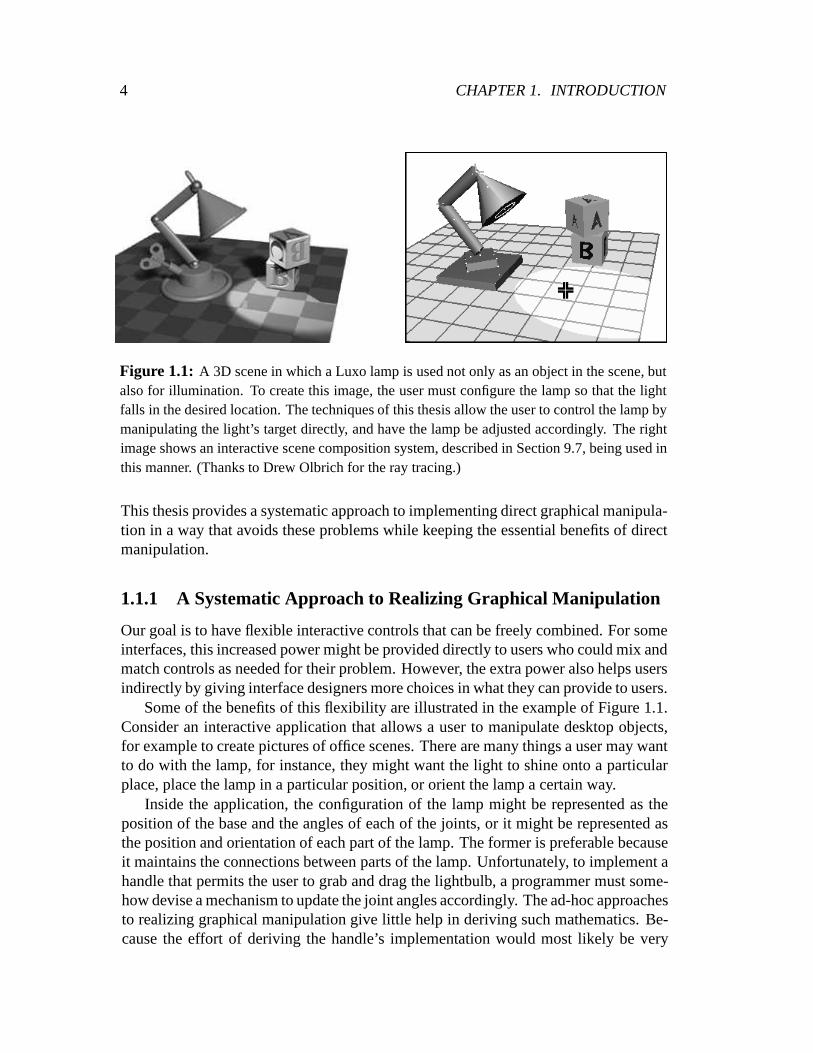
Figure 1.1: A 3D scene in which a Luxo lamp is used not only as an object in the scene, butalso for illumination. To create this image, the user must configure the lamp so that the lightfalls in the desired location. The techniques of this thesisallow the user to control the lamp bymanipulating the light’s target directly, and have the lampbe adjusted accordingly. The rightimage shows an interactive scene composition system, described in Section 9.7, being used inthis manner. (Thanks to Drew Olbrich for the ray tracing.)
This thesis provides a systematic approach to implementingdirect graphical manipula-tion in a way that avoids these problems while keeping the essential benefits of directmanipulation.
1.1.1 A Systematic Approach to Realizing Graphical Manipulation
Our goal is to have flexible interactive controls that can be freely combined. For someinterfaces, this increased power might be provided directly to users who could mix andmatch controls as needed for their problem. However, the extra power also helps usersindirectly by giving interface designers more choices in what they can provide to users.
Some of the benefits of this flexibility are illustrated in theexample of Figure 1.1.Consider an interactive application that allows a user to manipulate desktop objects,for example to create pictures of office scenes. There are many things a user may wantto do with the lamp, for instance, they might want the light toshine onto a particularplace, place the lamp in a particular position, or orient thelamp a certain way.
Inside the application, the configuration of the lamp might be represented as theposition of the base and the angles of each of the joints, or itmight be represented asthe position and orientation of each part of the lamp. The former is preferable becauseit maintains the connections between parts of the lamp. Unfortunately, to implement ahandle that permits the user to grab and drag the lightbulb, aprogrammer must some-how devise a mechanism to update the joint angles accordingly. The ad-hoc approachesto realizing graphical manipulation give little help in deriving such mathematics. Be-cause the effort of deriving the handle’s implementation would most likely be very

1.1. IMPLEMENTING GRAPHICAL MANIPULATION 5
specific to the Luxo lamp, traditional2 direct manipulation systems would most likelybe forced to provide the user with only direct control over the joint angles. While thisis sufficient to configure the lamp, it is not necessarily convenient for tasks like posi-tioning the light bulb or aiming the light.
This thesis presents a systematic approach for implementing direct graphical ma-nipulation. A general-purpose mechanism maps between the handles provided to theuser and the parameters of the graphical objects. With such an approach, a user of theLuxo lamp example could not only manipulate the joint angles, but could also grab anypart of the lamp directly, The programmer did not have to explicitly code the math-ematics to map the manipulations into parameter changes. Infact, the flexibility incontrols permits definition of other less obvious handles that permit the user to havedirect control over attributes of interest. For example, a user interested in shining thelight onto a particular location could simple grab the target of the lamp (the center ofthe spot) and drag it to the desired location. The controls can be freely combined. Forexample, a user could position the light’s target and simultaneously specify the lamp’sposition on the table.
A systematic approach to realizing direct manipulation canbe based on a generalpurpose mechanism for mapping user controls to object parameters. Creation of sucha mechanism requires us to view graphical manipulation as a constrained optimizationproblem. To solve this problem in a practical manner, we musttreat itdifferentially,thatis to control how objects change rather than their final targets. This thesis introducesa differential approachto graphical interaction that begins by taking the view of ma-nipulation as a mathematical problem. To realize the approach, the thesis will providemathematical techniques to solve the problem, implementation techniques to addresspragmatic issues, and a system architecture to use the approach to build applications.Example interaction techniques will be provided to show thepromise of the approach,and applications will be demonstrated to show its viability.
1.1.2 Classes of Users and Tools
There are different classes of people involved with an interactive graphical application.As in Myers’ survey [Mye93], we will need to distinguish these into distinct categories.Myers’ categories are users, interface designers, application programmers, and tool cre-ators. For the purposes of this thesis, we will lump interface designers and applicationprogrammers together as their tasks are similar: to build the application that the userwill employ in their graphical task with the tools provided by the tool creators. Theapplication builders will be the users of application development tools, but unless we
2The Luxo lamp is an example of an important special case: an articulated figure. Recently, sev-eral commercial animation systems, such as SoftImage [Sof93] and Wavefront [Wav94], have includedinverse kinematic techniques to manipulate such objects bypositioning end-effector points. These meth-ods, and their limitations, will be reviewed in Section 2.2.4.

6 CHAPTER 1. INTRODUCTION
explicitly refer to the “user of the toolkit,” the term “user” will refer to the “end user”of the graphical application.
The work of this thesis affects all three groups. While our approach can be em-ployed to provide conventional interfaces, it may also be used to provide new types ofinterfaces for users. It gives the application programmer anew set of abstractions withwhich to build interactive systems. Finally, for the toolkit builder, there is a new classof services that must be provided, but these services can help enhance the modularity ofthe tools by: providing a standard interconnection mechanism between objects; allow-ing the internal representation of the objects to be hidden from applications program-mers; allowing tools to be provided to the application programmer that allow piecesto be assembled by combination and composition to form interaction techniques; andallowing the encapsulation of numerical constraint computations.
One might consider applications where the user is exposed tothe mathematics be-hind their graphical application. For example, the CONDOR system [Kas92] allowsthe user to construct mathematical expressions that define the graphical objects. Al-though such an application can be constructed using the approach of this thesis, thisthesis focuses on applications where the user is insulated from the mathematics, in-stead directly manipulating graphical objects. In fact, a goal of this thesis is to hide asmuch of the mathematics as possible inside the applicationsdevelopment tools so thatonly the tool creators need see it.
1.1.3 Graphical Manipulation as Equation Solving
To introduce the differential approach of this thesis, graphical manipulation must beviewed as a constrained optimization problem. Graphical manipulation deals with howa user configures a set of graphical objects to achieve some desired goals. For the lampexample, the set of graphical objects consists of the Luxo lamp, the table top, and theother objects on the table such as the blocks. I will often usethe termmodelto refer tothe set of objects.
In the class of graphical manipulation tasks considered in this thesis, users manipu-late objects whose configurations can be stored as a concise set of real-valued parame-ters, called the object’sstate vector.For a given object, there are potentially many setsof parameters which might equivalently serve as a representation, as demonstrated bythe line segment example. Aparameterizationis a particular representation of the stateof an object.
Objects usually have many attributes that may be of interestto an observer. Since,by definition, the state vector fully describes the configuration of the object, the at-tributes must be determined as functions of these parameters. For this thesis, we re-strict ourselves to the broad class of object attributes which can be computed by closed-form, differentiable expressions over the state variables. This class includes many ofthe types of models used in interactive computer graphics such as most parametric and

1.1. IMPLEMENTING GRAPHICAL MANIPULATION 7
implicit curve and surface representations, transformation hierarchies, virtual cameras,and many simple shading models. We will not consider things such as combinatorialor discrete attributes, such as the number of sides of a polygon, or attributes computedby recursive or iterated functions such as fractals.
A control is an attribute of an object that can be specified or directly manipulated.For example, if a system allowed the user to drag the positionof the lamp’s lightbulb orthe target location of the light, these attributes of the lamp would be serving as controls.A constraint is a control for which a fixed value is given, preventing the value of theattribute from changing. Such controls constrain the behavior of objects by restrictingtheir motion so that the constraint is not violated. For the purposes of this thesis, theterms constraint and control are nearly interchangeable: aconstraint is a control withits value fixed, a control is a constraint whose value is beingspecified dynamically bythe user, e.g. a value constrained to follow the mouse.
A single control generally does not uniquely determine a configuration of the object.For example, if one endpoint of a line segment is specified, there is still a continuum ofpossible configurations for the segment. To combat suchunder-constrainedsituations,it is often desirable to use multiple controls simultaneously. In the cases where there isonly a single input device, dragging manipulation might be combined with constraints(e.g. controls that are restricted from changing). In a sense, even a single draggingoperation can be thought of as multiple controls if we consider each axis of the pointingdevice independently.
It is unreasonable to require the user to employ enough controls to uniquely de-termine the configuration of the graphical objects. The usersimply may not know orcare about some attributes of some objects, or it might be toomuch work to specifyeverything. In such under-constrained cases, the system must somehow choose one ofthe possible configurations. Without mind reading, it is impossible to reliably selectthe solution that the user most desires. Systems must settlefor simply trying to select asolution that is reasonable. One version of this is the “Principle of Least Astonishment”[BDFB+87] which suggests the system should try to select the optionthat will surprisethe user the least.
For an analogy, think of a model as a large machine which has a few knobs for theuser to turn and many gauges whose values the user may be interested in. Supposethere are a few gauges for which the user desires a particularvalue. The graphicalmanipulation task is to find settings of the knobs such that the gauges reach these desiredvalues. If each gauge to be specified corresponds directly toa knob, the task is easy,because each knob can be turned and set independently. However, most gauges willdepend on complicated combinations of the knobs, making it harder to find settings ofthe knobs that achieve desired values. In this metaphor, theknobs are the parametersof the graphical objects, the gauges are attributes of the objects that the user may beinterested in, and the internals of the machine correspond to the functions that computethe attributes from the parameters. Traditional implementations of direct manipulation

8 CHAPTER 1. INTRODUCTION
require the user to control the knobs directly. The methods of this thesis permit the userto use any of the gauges as controls by automatically adjusting the knobs as needed.
1.1.4 Goals for Graphical Manipulation
Treating interactive control as the specification of valuesfor controls as in the lastsection leads to a concise mathematical problem. The user would like to specify someset of controls,p. The system needs to find some configuration of the state variables,q, which meets this. Since the controls can be computed as a function of the statevariables, we have
p = f(q): (1:1)
Solving the manipulation problem is, at one level, as straightforward as solving thisequation forq . However, there are many difficult goals which we might want oursolution technique to meet:
1. flexibility in the types of controls, and therefore the functions which computethem;
2. freedom to combine controls arbitrarily, “mixing-and-matching” them dynami-cally;
3. keeping the good properties of direct manipulation, e.g.continuous motion, rapidfeedback, tight coupling of the input device to objects on the screen,: : : ; [Sch83]
4. choosing the “best” solution in under-constrained cases, and finding a “reason-able” answer even if there is no exact solution.
To aid the application implementor, there are several othergoals:
5. freedom in picking representations independently of user concerns;
6. a standard procedure for defining new controls that minimizes the amount ofdifficult mathematical work in defining a new type of control;
7. a solving mechanism that is general purpose and encapsulatable so that a singlecommon implementation can serve a number of applications and so that the ap-plication developers need not worry about the details of thesolving mechanisms.
We would like the techniques developed to realize the approach to also:
8. work over a variety of domains;
9. be fast and scale well;
10. require only readily available, easy to code numerical algorithms. Reliance onsophisticated numerical codes that must be purchased from commercial vendorsor developed by expert numerical analysts would be unacceptable.

1.1. IMPLEMENTING GRAPHICAL MANIPULATION 9
1.1.5 The Problems of Other Approaches
Our goals make solving Equation 1.1 forq impractical for three general reasons:
� in order to have flexibility in the types of controls, non-linear equations may needto be solved. Such equations are hard to solve;
� in order to have flexibility in the number of controls that arespecified, we mustpermit under-constrained and over-constrained cases;
� in order to provide the desired direct manipulation interface, object must movewith continuous motion. Therefore, the solver must be fast enough and providecontinuity in the solutions.
In order to provide direct manipulation with general controls by solving Equation 1.1,we must solve arbitrary systems of non-linear equations fast enough to allow for fre-quent enough updates to give the user the illusion of continuous motion.
In order to meet goal 1, the equation solver must be able to handle a wide range offunctions, including non-linear equations. Without knowledge about the functions to besolved, sets of equations are difficult to solve. Not only is good information hard to findin general, but each combination of equations might also require specific knowledge.Because of this, [PFTV86, Chapter 9] argues that not only does no reliable, general,non-linear solver exist, but that one cannot exist.
Without global information about functions and combinations, solving techniquesmust rely on local information, effectively searching for solutions. Almost all non-linear solvers are iterative methods that take an initial guess as to the solution andrepeatedly update the guess until they find a solution. Such asolver can never determinethat there is not a solution: if it fails to find a solution it might simply mean that it hasnot searched hard enough. These solvers will be discussed further in Section 2.2.2.
As computers grow faster, it might become practical to consider using a sophis-ticated non-linear equation solver to provide direct manipulation. However, such anapproach is unlikely to succeed for a number of reasons:
� despite their sophistication, the methods are heuristic and not completely reliable;
� because they are doing searches, it is difficult to predict how long it will takethem to find a solution;
� the solvers may fail to find a solution, but only after spending a long time lookingfor it;
� the solvers do not degrade gracefully: it is difficult to limit the amount of timethat they spend because their intermediate states may not beclose to the answer;

10 CHAPTER 1. INTRODUCTION
When we examine the previous approaches to implementing graphical manipula-tion, we see that they all fail to meet some of these goals. Previous work will be ex-plored in more detail in Chapter 2.
Traditional Direct Manipulation – The traditional method for implementing directgraphical manipulation has been to couple parameters directly to the pointingdevice. For example, with the luxo lamp, a conventional direct manipulationsystem would allow the user to connect a joint angle to a knob.Some mappingsbetween the input and the values are possible, for example toconvert the linearmotion of a slider to the rotary motion of the joint, but theremust be some directway of computing the parameter values from the inputs.
Traditional implementations have been the mainstay of direct manipulation inter-faces. Such interfaces have been very successful, largely due the fact that it meetsgoals 3 and 9. However, its limitations have restricted the types of interfacesthat have been constructed. Traditional direct manipulation severely restricts thetypes of functions which can be used as controls (goal 1) and it provides no au-tomatic way to combine controls (goal 2). Parameters must bechosen so thatthe controls will map onto them easily (failing goal 5). Because good represen-tations must be developed for any new controls, and because these closed formmapping for controls must be found, developing new controlscan be difficultwork (violating goal 6).
Parametric Modeling Approaches – Parametric modeling is a variant of the tradi-tional direct manipulation approach. Such schemes permit end users to createmodels with parameter dependencies. These parameters are directly specified.Parametric approaches permit a clever user to overcome someof the deficienciesof the traditional direct approach. For example, if the designer of the Luxo lampknew the user would want to control the height of the lamp, butnot the jointangles, they might have devised a way of representing the configuration of thelamp so that height is a parameter, and the joint angles are computed from that.Parametric approaches suffer from the same failures of direct manipulation, al-though it does permit a clever user to sometimes have some additional flexibilityin the types of controls.
Traditional Constraint-Based Approaches – A constraint-based interface3 treatsEquation 1.1 by employing an equation solver. Typically, the user specifies val-ues for various aspects of the model and then the system solves for some value ofthe state vector which meets these constraints. We call sucha constraint-basedapproach a “specify-then-solve” style.
3I use the termconstraint-basedinterface to mean that constraints are an abstraction provided to theend user of a system, rather than simply as an abstraction used by programmers.

1.1. IMPLEMENTING GRAPHICAL MANIPULATION 11
Although the problem of solving the equations required to meet goals 1 and 2is difficult, a bigger problem with a specify-then-solve approach is that it failsto meet goal 3. After the user specifies the constraints, the system solves theequations and then displays the result to the user. Objects jump to the new con-figuration, leaving the user to puzzle out what happened. This makes goal 4 evenmore difficult. It becomes critical to pick a good solution toavoid confusing theuser. Picking the correct solution is also important because without the rapidfeedback of direct manipulation it can be difficult to explore possible solutions.
A system designer might consider using interpolation to provide the desired con-tinuous motion in a constraint solving system. After solving for a new configu-ration a system might make a smooth transition by interpolating between the oldstate and the new. However, jumping between configurations cannot be avoidingby simply interpolating. Unless something enforces the constraints in the inter-mediate states, the constraints may be broken, leading to potentially undesirablebehavior.
Specialized Constraint-Based Approaches –The primary drawback of the tradi-tional constraint-based approach is that it violates goal 3, the desire for directmanipulation. One approach to handling this is to restrict the class of constraintsso that they can be solved faster. The best examples of this are the propagationconstraint solvers, such as DeltaBlue [FBMB90]. In essence, these algorithmstrade-off goals 1 and 2, in order to better meet goal 3. As a side effect, some ofthese algorithms provide techniques, such as constraint- hierarchies [BFBW92],to handle under-constrained cases (goal 4). Unfortunately, propagation solversrestrict the set of possible controls and the ways controls can be combined in waysthat are unacceptable for graphical manipulation (failinggoals 1 and 2). Also, foreach new control, a variety of bi-directional methods must be generated, whichmay not be easy for many types of functions (failing goal 6).
The problem of determining configurations that achieve the desired attribute val-ues is an important problem in robotics and computer animation. Such solving isreferred to asinverse kinematics.The inverse kinematics literature, examined inSection 2.2.4, includes numerical methods that solve the systems of non-linearequations. A problems of particular interest to robotics, namely configuring artic-ulated figures by positioning end-effectors, is particularly well-studied. Highlydeveloped techniques have been developed and are commonplace enough to besurveyed in robotics textbooks, such as those by Craig [Cra86] or Paul [Pau81].The techniques are now appearing in commercial computer animation systems,such as Softimage [Sof93] and Wavefront [Wav94]. The methods in such sys-tems are not general: they only permit manipulation of a veryspecific controlon a very specific class of model (failing goals 1, 5 and 8), andtypically provideonly a single control at a time (failing goal 2). The differential approach can be

12 CHAPTER 1. INTRODUCTION
viewed as a use of generalized inverse kinematics to create ageneral approachto implementing graphical manipulation.
1.2 The Differential Approach
Existing approaches fail to meet the goals for graphical manipulation, demanding thedevelopment of a new approach. An advantage that we have overthe developers of pre-vious approaches is that computer hardware has advanced to the point that the machineson which graphical applications are run have considerable computational and graphicsperformance. Such machines make it possible to do non-trivial numerical calculationsin between each frame of continuous motion animation. This means that it is possible toperform some numerical constraint calculations and still provide a continuous-motiondirect manipulation interface. This thesis presents such an approach to graphical inter-action.
Our goals make solving the manipulation problem of Equation1.1 difficult. Pre-vious approaches have either restricted the equations, or restricted the desired directgraphical interaction. In this thesis, I will present an approach which makes a differ-ent kind of restriction: that we are interested only in direct graphical interaction andwill always demand that objects move with continuous motion, not jump between verydifferent configurations. The interfaces desired for graphical interaction have this prop-erty.
Because we are considering cases where objects move continuously, it is sufficientto control them by controlling how they change over time. By controlling how objectsare changing, rather than controlling their configurationsdirectly, a variant of Equation1.1 may be solved. Controls specify the attributes’ rates ofchange and the systemsolves for the state variables’ rates of change to make this happen. I call this approach tographical interaction based on this control by time derivatives thedifferential approach.
With the differential approach, at particular instants in time a solver must determinethe time derivatives of the state vector given the time derivatives of the controls. Werefer to this asdifferential optimization.Solving the differential optimization is a muchmore mathematically tractable problem than solving Equation 1.1 directly. This meansthat it is possible to provide direct graphical interaction(meeting goal 3), while han-dling a general class of non-linear functions (meeting goal1), and allowing these to becombined in arbitrary ways (goal 2). Methods for solving thedifferential optimizationproblem address the issues of under-constrained and over-determined cases (goal 4).
The differential approach meets the implementation goals as well. By allowingalmost arbitrary non-linear functions to map between controls and parameters, it pro-vides flexibility in selecting representations of objects independently of how they willbe manipulated (goal 5). The solving methods require littleinformation about the con-trol functions, in fact, all that is required can be found automatically given the control

1.2. THE DIFFERENTIAL APPROACH 13
function (goal 6). The mechanisms behind the differential approach are general purposeand can be encapsulated in a manner that not only hides the underlying mathematicaltechniques, but also permits a single implementation to serve as a building block foralmost any type of system requiring graphical manipulation(goals 7 and 8). The tech-niques to realize the approach perform well enough to work oncurrent machines (goal9), without resorting to numerical routines beyond those instandard textbooks (goal10).
1.2.1 Direct Manipulation in the Differential Approach
Digital computers provide the illusion of continuous motion of graphical objects byrepeatedly redrawing the image. The time between these redraws must be sufficientlysmall in order for the illusion to be maintained. To support direct manipulation, asystem must sample the position of the mouse and update the positions of the objectsat a rapid rate.
The differential approach breaks the numerical constraintsolving problem into twoparts: computing the rates of change of the parameters at particular instants, and com-puting the trajectory of the parameters over time, given therates of change at particularinstants. The former problem is the differential optimization problem, and the latter issolving an ordinary differential equation (ODE). Between each redraw, the ODE mustbe solved to update the configurations of the graphical objects. Each of these solversteps advances the configuration by solving some number of differential optimizations,each determining the rate of change at some particular instant.
With the differential approach, the graphical objects cannot simply be moved withthe mouse. Instead, each step they move towards a target. Limitations in ODE solving,discussed in Section 3.3, provide speed limits on how quickly objects can move, so theymay not be able to reach their target in the time provided. If the target is the position ofthe mouse, this will cause the object to lag behind its target, gradually catching up asthe mouse slows down. This can make manipulation feel as if the objects are connectedto the input devices by springs, and will be discussed in Section 6.1.2. As computersgrow faster, more computation can be done between each redraw while maintaininga rate sufficient to provide the illusion of continuous motion. This allows raising theeffective speed limits of the objects, and can reduce the lag.
1.2.2 An Alternate View of Graphical Manipulation
An alternatative view of graphical manipulation is to imagine graphical objects as phys-ical entities that are manipulated as physical objects in the real world: by pushing andpulling on them. With such a view, implementing direct manipulation becomes a prob-lem of implementing an interactive physical simulation. The issues in creating such

14 CHAPTER 1. INTRODUCTION
simulations are explored by Witkin et al.[WGW90]. The techniques presented in thatpaper form the basis for this thesis.
The differential approach can be viewed as a variant of the physical simulationapproach. The physics of the “world” is modified from that of the real world in orderto facilitate manipulation. Most significantly, inertia isremoved by replacing Newton’slaw of motion,f = ma; by its first derivative equivalent,f = mv: An object in motionis only in motion while it is being acted upon by a force. For manipulation, this has theadvantage that objects remain where they are placed, ratherthan skidding around.
The mathematical methods used for implementing the differential approach pre-sented in Chapter 3 are the same as those used for implementing physical simulations.Many of the numerical methods and implementation techniques in the thesis were orig-inally conceived for implementing interactive simulations. Presenting the differentialapproach as constrained optimization, as done in this thesis, rather than presenting it asa physical simulation, is largely a matter of taste.
1.3 An Approach to Graphical Interaction
The ultimate goal of this research is to improve the quality of graphical manipulationinterfaces. The central focus of this thesis makes an indirect step towards this goal,providing a new set of abstractions which provide more flexibility in the type of inter-action techniques that can be created. This increased flexibility does not necessarilyimply better interfaces — in fact, they give interface designers new ways to baffle andconfuse users. However, there are several reasons to believe that the differential ap-proach can lead to improved interaction techniques.
The differential approach permits building interfaces which have many desirableproperties. It provides for continuous motion of the graphical objects. It permits in-terfaces to provide controls to the user which permit directly controlling attributes ofinterest. These controls need not directly connect to the parameters. It permits controlsto be combined, either by the user or by interface elements.
The example interaction techniques of Chapter 8 show the promise of the approach.The examples which recreate prior techniques show that the abstractions provided bythe differential approach are sufficiently rich to create usable interactions. Some of thenewer techniques, such as the through-the-lens camera controls of Section 8.1.4 couldnot have been considered with previous approaches to building interfaces. Some ofthe examples, like the artificial horizon of Section 8.3.5, are not good interfaces. Butwith the differential approach, techniques can be exploredwithout deriving the inversemathematics, so it is possible to learn that they are unusable before investing a largeamount of time and effort in their development.
The differential approach provides a new set of abstractions for building graphi-cal interaction techniques. In the remainder of this section, we briefly introduce the

1.3. AN APPROACH TO GRAPHICAL INTERACTION 15
Line State Vectorx1 y1 x2 y2
left right center length angle
l θx y x y x y
Figure 1.2: A schematic representation of a simple graphical object. The object stores a setof parameters internally in itsstate vector.However, the outside world accesses the object viaits connectors, providing flexibility and parameter independence.
abstractions, along with the terminology used throughout the thesis.
1.3.1 Graphical Objects and Connectors
For the purposes of this thesis, we are concerned with what are commonly calledobject-orientedgraphical editors. In such applications, the user deals with finite sets of graph-ical objects which must be manipulated to create the desiredmodel or drawing.
For the most part, graphical objects are the visible entities that the user manipulates.However, we will consider structural elements, such as the groups that aggregate ob-jects or the viewing transforms that map virtual worlds to screen coordinates as objectsas well.
For a graphical object, there are two “sides” which we must consider. On one handis what the programmer “sees,” the object’s internal representation. An important partof this are the parameters that determine the configuration of the object. Each objectstores this set of numbers as itsstate vector.
To the user, the graphical object should appear as a graphical object. We assumethat the user is interested in the graphical entity, not in the internal data structures usedby the programmer. For any object, there are many attributesthat may be of interest tothe user, or to other objects in the program for that matter.
Ideally, we would like to think of a graphical object as a sealed box. Inside is theprogrammer’s internal representation, including the state vector. To the outside world,all that is visible are the many attributes which other partsof the program, or the user,may want to observe. Our desire to think this way leads us to draw graphical objectsschematically as Figure 1.2. The central notion is that the state is internal to the objectand the object’s “outputs” are its attributes. How the object computes these attributesis the concern of the object itself, not the outside world.
The state vector of an object fully specifies its configuration. Therefore, any at-tribute of the object must be a function of these variables. This function must be known,otherwise it would be impossible to compute the value of the attribute.
A graphical object may know how to compute many attributes. The set of attributes

16 CHAPTER 1. INTRODUCTION
of an object is not necessarily fixed — an object may have many attributes, and newattributes may be created in response to the needs of some other part of the system orthe user. The schematic of Figure 1.2 may be slightly misleading in that it should notimply that the depicted outputs are a fixed, small set.
We will call the outputs of graphical objectsconnectors.As the name implies, theseare the sockets into which the outside world will connect to the object. A connectoris an attribute that an object provides for the outside worldto access. Throughout thisthesis, the notion of connector will be both a conceptual idea as well as a data structurethat realizes it.
1.3.2 Compound Objects and Dependencies
Many attributes can be computed as functions of other attributes, rather than from insidethe object. For example, if we wish to know the length of a linesegment, this attributecould be computed as a function of the positions of endpoints. Therefore, if the linesegment did not know how to produce its length as a connector,we might create aspecial ruler object that looks at the positions of two points and “connect” it to theendpoint outputs of the line segment.
An important notion in the ruler example is that the ruler object takes as its “inputs”the “outputs” of another object. The ruler measures the distance between two points,without concern for what these points are. This is significant for three reasons:
� It means that the objects, such as the line segment, can be extended to have newbehaviors without being internally modified.
� It means that we need only one type of ruler, no matter how manydifferent typesof objects we might be measuring.
� We are not necessarily restricted to points on a single object. Instead we couldmeasure the distance between two points on two different objects.
Objects like the ruler have inputs that plug in to the output connectors of othergraphical objects. Considering such dependencies leads usto draw schematic diagramssuch as Figure 1.3. The outputs of the connective objects areattributes just like theoutputs of the simpler objects. The distance output of the ruler should be a first-classcitizen, just as the position outputs of the line segments. Like the outputs on simplerobject, the connectors on the ruler object’s outputs are also functions of the state vector,except that they are potentially functions of the state vector of the entire model (whichwe will call theglobalstate vector), rather than just the state vector of a single object.The function that determines the attribute’s value can be built by composition: firstcomputing the values of the inputs and then using these values as the inputs to a functionwhich computes the distance.

1.3. AN APPROACH TO GRAPHICAL INTERACTION 17
Line State Vectorx1 y1 x2 y2
left right center length angle
l θx y x y x y
dist.
d
Line State Vectorx1 y1 x2 y2
left right center length angle
l θx y x y x y
Ruler
Figure 1.3: Compound objects are composed by plugging objects’ connectors into sockets,like wiring together a circuit. A standardized protocol allows independence in wiring.
This picture emphasizes an important notion in the thesis: the idea of pluggingobjects into the “outputs” of other objects. The facility todynamically plug and unplugsuch connections in response to user actions or other systemevents is an essential partof the differential approach, and will figure prominently inthe design of the machineryto realize it.
The key element for creating the vision of snap-together objects in the differentialapproach is a standard protocol for the outputs so that anything can be plugged in.Since the connector outputs are primarily functions, the aggregate connection operationis function composition: building more complicated functions from simpler pieces.By supporting this operation in a dynamic environment, the machinery to realize thedifferential approach can permit the needed plugging and unplugging.
Compound objects, like the ruler, can come in many forms. Typically, they are usedto compute aggregate properties of many different objects.For example, the distancebetween two points, or the relative orientation of two line segments. They may alsobe used to compute conversions, for example from degrees to radians. More complexattributes can also be built this way, for example, we might compute the position of ashadow as a compound operation that takes the position of a point, the position of alight source, and the position of the floor as its inputs. Flexibility in building new typesof attribute outputs is a useful feature of the differentialapproach.

18 CHAPTER 1. INTRODUCTION
Line State Vectorx1 y1 x2 y2
left right center length angle
l θx y x y x y
Line State Vectorx1 y1 x2 y2
left right center length angle
l θx y x y
diff.
x y
x y
Attach
FollowMouse X
FollowMouse Y
GoTowards0
GoTowards0
GoTowards3
Figure 1.4: Objects are manipulated by attaching controllers to their connectors. A controllerspecifies how the value of a connector should be changing. Controllers can be plugged intoany connector. This diagram represents a model with two linesegments that are attached. Onesegment has its length constrained, while the other is beingdragged.
1.3.3 Control of Graphical Objects
Since the attributes are the only view of an object that the programmer is given, itfollows that these attributes must also serve as the handlesby which the object is con-trolled. The vision of the differential approach is that anyattribute output should beable to serve as a mechanism to control the object, and that these controls should beable to be freely applied as needed in any desired combination. Thus, any output shouldalso be able to serve as an input.
Our notion of using an output as an input can be best discussedby introducinganother kind of special object, thecontroller. A controller is a simple object that plugsinto a connector and specifies what behavior the outside world desires from it. Withthis final abstraction, we are led to draw schematics such as Figure 1.4.
With the abstractions in place, we can now examine Figure 1.4to see the mathemat-ical constraint problem. We have specified the outputs of thefunctions that compute
1.3. AN APPROACH TO GRAPHICAL INTERACTION 19
the attributes being used as controls, and must determine the inputs to these functions(the value of the state vector) to achieve the desired values.
As discussed in Section 1.2, we cannot solve this constraintproblem directly. In-stead, we will solve it differentially. This means that rather than specifying desiredvalues for attributes, controllers specify how they shouldbe changing over time. Acontroller specifies a rate of change for the attribute it is connected to.
It is important to notice that the controllers cannot instantaneously affect the valuesof the connectors they control, nor the state variables of the objects. Instead, theyspecify how those connectors are changing, and over time, those changes will takeeffect. This implies that there is a continuous flow of time over which the controllerscan act. At discrete instants, the set of active controllersmay be altered, but valuescannot be changed.
What a controller can do is quite limited: it can simply specify the desired rate ofchange of an attribute. The diversity of interaction techniques comes not from diver-sity in the types of controllers, but rather, from the way they are applied. Interestinginteraction techniques result from:
� attaching controllers to interesting attributes;
� connecting controllers at interesting times;
� using controllers in interesting combinations.
Interaction techniques are defined by controlling connectors over time. For exam-ple, to drag a point, the connector that computes the point’sposition is connected to acontroller when the mouse button is pressed to initiate the drag, and the controller is re-moved when the mouse button is released. Similarly, a mechanical connection betweentwo points is created by using an object which computes the displacement between twopoints and creating a controller which drives the displacement to zero.
The differential approach provides a basic set of abstractions from which interfacesand interaction techniques can be built. The ability to wiretogether attributes and attachcontrollers to them provides machinery that can be applied in a wide variety of manners.
One interface style which is enabled by the differential approach is to provide theabstractions directly to the user, permitting them to mix and match controls as needed.For example, in the lamp demonstration, the user would be permitted to grab and dragmany points involving the lamp, including the light’s target, the bulb, and the cornersof the base. Attributes which are not positional, such as joint angles or bulb brightness,might be connected to sliders. The user could configure the lamp by manipulating anyof these controls, or by constraining their values. Controls are mixed-and-matchedby manipulating or locking their values. This interface style is similar to a traditionalconstraint-based interface. Many of the issues which make constraint-based interfacesdifficult to design must be addressed, such as how to present the palette of options tothe user effectively.

20 CHAPTER 1. INTRODUCTION
Another way that the differential abstractions may be employed is to build interac-tion techniques which are more similar to the traditional direct manipulation interfaces.An example is the 3D translation widget discussed in Section8.3.6. To the user, thetranslation handles appear as they do in other systems whichprovide them. However,this interaction technique can be concisely described by defining sets of controllersduring dragging. While the differential approach is merely used to recreate an existingtechnique in such cases, it does have some interesting benefits. The differential ap-proach addresses the difficult question of how to define such interesting behaviors in away that is parameter independent, and easy to generalize toother controllers.
1.3.4 Impact on Application Architecture
Just as the differential approach frees the user from worrying about the object repre-sentations, it can also hide such parameterizations from the programmers of graphi-cal applications, helping to foster encapsulation. Objects merely expose mathematicalfunctional outputs for attributes that other pieces of the system may be interested in.The program manipulates the object by placing constraints and controls on these ports,and the differential solving mechanism takes care of adjusting the parameters accord-ingly.
The solving mechanism needs very little information about the functions that arebeing constrained and controlled. This means that objects need not expose much infor-mation about the functions they provide. It also simplifies the composition of functionsfrom pieces, such as object outputs. This allows creation ofa utility which permitsfunctions to be defined dynamically, for example in responseto user actions. The corefunctionality of the differential approach, the ability todefine functions and place con-straints and controls on them, can be built in a general purpose manner.
The general protocol for connecting the outputs of objects permits the creation ofgeneral purpose objects, constraints, and interaction techniques. Objects can providemathematical ports without regard for what will “plug-in” to these ports. Constraintsand interaction techniques can be defined in terms of types ofoutputs, without regard forthe objects that are being connected to. For example, we define graphical objects thatproduce outputs that are the positions of points, and define constraints and interactiontechniques in terms of point position outputs.
1.4 Thesis Roadmap
This thesis introduces the differential approach, presents techniques to realize it, andprovides examples to illustrate its power and viability. Following this introduction, thethesis proceeds to review some relevant related work.
Chapter 3 introduces the basic set of mathematical techniques required to realize

1.4. THESIS ROADMAP 21
the differential approach. The methods treat manipulationas equation solving. Thisproblem is handled differentially to make it feasible to solve. The fundamental com-putation is solving a constrained optimization problem to compute how the parametersof objects are changing given the rates of change of the controls. Basic methods forsolving these constrained optimization problems are developed and extended to handleunder- and over- constrained cases. The chapter also considers how to use the computedrates of change to actually create the motion, a problem of solving ordinary differentialequations from initial values. The chapter concludes with asimple example, workedthrough in detail.
In order to use numerical techniques in an interactive system, there are two centralchallenges that must be faced. The computations must be madeto go fast enough, andthe computations must be defined dynamically in response to the users actions. Theseissues are considered in Chapter 4 and Chapter 5 respectively. Chapter 4 considersmethods to achieve the needed performance in such solving. After analyzing the com-putational bottlenecks of the approach, a variety of methods are presented to enhanceperformance. One key element is exploiting the inherent sparsity of systems of equa-tions to be solved. Other techniques include solving smaller problems while still givingthe user the illusion that the system is solving a larger problem, and trading unneededaccuracy for speed.
Chapter 5 considers the task of dynamically defining functions in a way that they canbe rapidly evaluated with their derivatives. A tool called Snap-Together Mathematicsthat allows functions to be built dynamically from smaller pieces is presented. Snap-Together Mathematics is an important element of the differential approach becauseit provides the software structure for dynamically mixing and matching controls, andprovides a mechanism for encapsulating the mathematics of the approach.
With the basic machinery in place, Chapter 6 considers how the tools are appliedto create interaction techniques. It defines the set of abstractions provided to inter-face designers by the approach, and describes how the differential notion of time isdifferent than what is commonly used in interactive-systems programming. The chap-ter provides some basic examples of how the abstractions areemployed, and providessome extensions to the basic differential techniques to permit such things as inequalityconstraints.
Chapter 7 discusses how the differential approach can be encapsulated into a graph-ics toolkit. The Bramble toolkit was designed to aid in the development of graphicalediting applications with the differential approach. Various elements of the toolkit aredescribed, with an emphasis on how it supports the differential approach.
Chapter 8 describes interaction techniques built using theabstractions of the differ-ential approach. It begins by discussing some basic strategies. It then provides concreteexamples of techniques to address various interaction tasks. In addition to several novelinteraction techniques, many previous techniques are recreated, in order to show howthe Differential Approach can be applied to these problems.

22 CHAPTER 1. INTRODUCTION
Chapter 9 presents some example applications built with theapproach. The appli-cations serve to demonstrate the viability of the approach and to give some idea of itspromise in constructing tools for users. Chapter 10 concludes the thesis by summariz-ing the contributions, evaluating the various contents, and suggesting some directionsfor future work.
1.5 The Thesis
It is the premise of this thesis that:
� The numerical and graphical performance of modern processors can be appliedto address issues in graphical manipulation.
� A differential approachto graphical interaction provides a systematic implemen-tation of direct manipulation. This approach allows a system to provide userswith a broad class of interactive controls that can be freelycombined, yet pre-serves direct manipulation, so it does not suffer from the drawbacks of otherprevious approaches.
� Mathematical techniques to realize the differential approach can be provided,and that these techniques can be realized such that the issues of interactive sys-tems are addressed. In particular, methods permit the computations to be defineddynamically in response to user actions and to be performed sufficiently fast oncurrent generation hardware.
� The techniques of the differential approach can be encapsulated, providing a setof abstractions with which to build interfaces as well as a general purpose imple-mentation.
� The differential approach can have a positive impact on the way that interactiontechniques are developed and that interactive systems are constructed, by help-ing separate manipulation from representation and by enabling general purposeconstraints and interaction techniques.
� The differential approach can lead to interesting new interaction techniques andapplications, but can also serve as a substrate for implementing existing popularinteraction techniques.
1.5.1 Contributions
The contributions of this thesis are detailed in the final chapter. Briefly and generally,the contributions of this thesis are (in the order they will be presented in the thesis):

1.5. THE THESIS 23
� To introduce a systematic approach to graphical interaction based on the use ofnumerical non-linear constraint techniques, which I call the differential approach.
� To present mathematical techniques for solving the particular constrained opti-mization problems encountered in using the differential approach.
� To provide techniques to implement these mathematical techniques that addressthe pragmatic needs of interactive systems.
� To provide a toolkit that encapsulates the differential approach, providing its fea-tures to application developers while shielding them from the details of its im-plementation.
� To provide new interaction techniques and examples to address problems facedby users of interactive graphical applications, and to showhow these techniquesfit in the context of graphical applications.
� To provide example applications demonstrating the viability of the approach.

24 CHAPTER 1. INTRODUCTION

Chapter 2
I think the past is behind us. Real confusing if it was not,but anyway.
— Blues TravelerBut Anyway
Related Work
The differential approach uses constraint techniques to realize graphical manipulation.Like other uses of constraints in computer graphics, the differential approach must ad-dress a number of challenges in applying, solving, and implementing constraints. Thischapter looks at previous work on applications of constraints and constraint solvingtechnologies. It then looks at previous work on the creationof toolkits for the con-struction of graphical applications, as the differential approach will be used to createsuch a toolkit in Chapter 7. Finally, previous work on particular 3D interaction prob-lems used as examples Chapter 8 will be examined.
Both the basic idea of graphical manipulation, and the use ofconstraints to enhanceit, date back to Ivan Sutherland’s Sketchpad system [Sut63]. Englebart pioneered themore general use of a graphical pointing device in computer interfaces, as chronicled in[Eng86]. The style of interaction in which a pointing devicecontrols a graphical objectin a tight coupling is commonly referred to as direct manipulation, a term generallyattributed to Ben Schneiderman [Sch83]. His classificationof interfaces in terms of theuser experience led to later attempts to better define it [WR87], and even to argumentsas to why such categorizations are not helpful [WG87].
2.1 Uses of Constraints in Graphical Applications
Constraints have been used in graphical applications in many ways. Some systemsprovide constraint-based interfaces, that is, the users ofthe system are presented withconstraints to use in completing their tasks. Constraint techniques have also been usedto aid the programmer of graphical applications, by providing them with a tool to use inthe construction of their systems. The two uses of constraints are orthogonal: it is com-mon to write an application with a constraint-based interface using conventional tools,and to use constraint-based tools to write applications with conventional interfaces.
25

26 CHAPTER 2. RELATED WORK
2.1.1 Constraint-Based Graphical Interfaces
The central idea of a constraint-based graphical interfaceis that the user is able to makepersistent constraints: declarations that the system maintains after they are specified.The canonical example application of a constraint-based graphical interface is drawing.In a constraint-based drawing program, the user specifies relationships among partsof the drawing as persistent constraints that the system maintains during subsequentediting. For example, a user can attach an arrow to an object,and the position of thearrow is altered as the object is moved.
Sketchpad pioneered direct manipulation permitting usersto directly manipulategraphical objects by dragging them with the light pen. It also introduced constraintmethods, permitting users to specify relationships between parts, for example that twolines should be parallel. Sketchpad would “relax” the drawing until the constraints weresatisfied, and continue to maintain the constraints during subsequent manipulations.
Since this ground-breaking application, graphical manipulation has been continu-ally refined and has become standard. Constraints have not been as successful. Const-raint-based approaches to drawing have been limited by difficulty in creating con-straints, solving them, and displaying them to users. Theseinterface issues, coupledwith implementation complexity and performance problems,have prevented the wide-spread acceptance of constraint-based systems.
There have been examples of research systems for constraintbased drawing suchas Juno [Nel85], IDEAL [VW82], HILS [Whi88], CoDraw [Gro89], PictureEditor[KNK89], HotDraw [FB93], and Magrite [Gos83]. A very different use of constraintsis shown in the PED picture beautifier [PW85] that automatically places constraints ona rough drawing and solves them to clean up the drawing. Another use of constraintsis in the Visio [Sha93] diagramming program which permits defining object semanticswith equations with a spreadsheet interface.
Recent developments such as constraint inferencing, more widely available solvingtechnology, and the faster computers capable of solving constraints at interactive rateshave renewed interest in constraint-based drawing. Systems such as Chimera [Kur93],Grace [Alp93], IntelliDraw [Ald92], Rockit [KLW92], DesignView [Com92], Con-verge [Sis91] and my own Briar (Section 9.1) all use constraint inferencing to coupleconstraints and direct manipulation.
Constraint techniques have also been applied in 3D systems.Although SketchpadIII [Joh63], the first interactive 3D application, did not have constraints, they are sug-gested as a requirement for future systems. The VariationalGeometry systems of Lin,Gossard and Light [LGL81] renewed interest in the use of constraint techniques fordesigning 3D objects. Bruderlin [Bru86] and Rossignac [Ros86] presented constraint-based solid modelers. Constraint-based solid modelers that use direct manipulationinput are presented by Sohrt and Bruderlin [SB91] and by Fa etal [FFD93]. DavidPugh’s Viking system [Pug92], uses constraints to maintaingeometrical relationships

2.1. USES OF CONSTRAINTS IN GRAPHICAL APPLICATIONS 27
defined by sketching. Converge [Sis91] models 2D and 3D objects with constraints.Constraint methods have been applied to surface modeling, allowing users to ma-
nipulate surfaces without seeing the underlying representations. Fowler [Fow92] andWelch, Gleicher and Witkin [WGW91] present simple constraintmethods for control-ling points on B-Spline surfaces. Celniker [CG91] describes methods that optimize ashape interactively, which are extended in [CW92] to a broader class of constraints.Welch and Witkin [WW92] extend this work to a wider variety of constraints that per-mit the user to stitch together pieces of surfaces.
The “energy constraints” work of Witkin et al.[WFB87] introduces the idea of mod-elling using arbitrary functions of objects as controls. Barzel [Bar92c] discusses thephilosophical attractiveness of using physical constraints for modelling.
Specialized interactive graphics systems use constraintsto help users manipulatecomplex objects. Mark Surles’ SCULPT system [Sur92a, Sur92c, Sur92b] permitsthe interactive manipulation of molecules. The Jack system[PB88a] uses constraintmethods to interactively position a human figure. In [PB91],the authors extend Jackwith more complicated constraints on human figures.
The differential approach and the tools created to implement it were heavily mo-tivated by the desire to build constraint-based applications and to study the issues in-volved. Seeing 30 year old films of Sketchpad inspired the desire to understand howthese techniques might apply in modern systems. The energy constraints work was alsoparticularly inspiring because it demonstrated the utility of a wide range of controls, acentral theme in the differential approach. Of the systems discussed, Briar, Convergeand Chimera best typify the applications motivating the differential approach.
2.1.2 Constraint-Based Tools for Building Graphical Applications
Tools for building graphical applications have employed constraints to ease the con-struction process, for example, by automatically maintaining consistency multiple rep-resentations of data or between views and data. The use of constraint methods to sim-plify the construction of graphical applications was pioneered by Borning’s ThingLabsystem [Bor81]. The early successors to Thinglab for constructing interfaces usingconstraints are surveyed in [BD86]. Barth’s GROW toolkit [Bar86] was another earlyuse of constraints to help the programmer lay out the variouselements of the interface.
The common use of constraint methods for maintaining consistency of data cantrace its origins to non-constraint-based methods. The Smalltalk Model-View-Con-troller model [KP88] for direct manipulation implementation provided the influence formany other systems, despite its late appearance in the published literature. The modeluses separate objects to handle input and output for application objects. A critical pieceto implement the model is a mechanism for dependencies: objects must be notified ofchanges to other objects, for example to update the display when appropriate. Thedependency mechanism is a simple form of constraints known asone-waybecause the

28 CHAPTER 2. RELATED WORK
data only flows one way in the constraint. Distinctions amongtypes of constraints willbe explained in the next section.
More sophisticated algorithms for creating one-way constraints were introducedlater, and lead to more general dependency mechanisms for interface toolkits. Forexample, Hudson’s incremental attribute evaluation [Hud91] was used to create theApogee toolkit [HH88]. Similar one-way mechanisms were used in other toolkits suchas Coral [SM88], MEL [Hil91], and Garnet [MGD+90].
Despite the simplicity and limited expressibility of one-way constraints, they arean extremely useful feature in interface toolkits. They aresufficient to update viewswhen data changes, keep dependant data consistent, and helpdesigners lay out inter-faces. Simple solvers are extremely popular because efficient and simple mechanismsfor creating them have been widely available. As developments in solvers make morepowerful techniques practical, newer toolkits explore their advantages. Examples in-clude Rendezvous [HBP+93], ThingLab II [Mal91], VB2 [GBT93], and Multi-Garnet[SB92]. Rendezvous even permits creating constraints across multiple displays, main-taining consistency between multiple users of a shared application.
The existing constraint-based tools for developing graphical interfaces are inade-quate for constructing the constraint-based applicationsand examining the interfacequestions I wanted to study. The lack of support for numerical constraints in existingtools provided a niche to be filled with the work of this thesis. It is important to explorewhether numerical constraint methods could be encapsulated and provided in a toolkit.
2.2 Constraint Solving Technologies
The wide array of uses of constraint techniques has led to thecreation of an even largerselection of constraint solving technologies. Here, we provide a brief survey. Mostsystems have only used a single solving technique. Other systems, including the earlySketchpad [Sut63] and ThingLab [Bor81], used hybrids wheremultiple solvers wereused to solve different parts of problems.
2.2.1 Propagation and Symbolic Methods
The simplest constraint methods allow the specification of dependencies among ele-ments of the data. Some mechanism is provided in order to makesure that dependentvalues are updated appropriately. These mechanisms can operate either by replacing ac-cesses with function calls to recompute the data, or by having changed data notify theirdependents. This latter approach is known aslocal propagationbecause new resultsfirst propagate to elements closely connected (i.e. local) in the dependency graph. De-pendency schemes are calledone-waybecause information flows only one way acrossthe dependencies. Despite their simplicity, one-way localpropagation techniques are

2.2. CONSTRAINT SOLVING TECHNOLOGIES 29
extremely popular because they are easy to implement efficiently and because they canprovide some important needs in user interface software, Efficient methods for handlingone-way constraints by minimizing the number of evaluations are discussed by Hudson[Hud91], and extensions to one-way constraints for indirectly referencing variables areprovided by Vander Zanden et al.[VZMGS91, VZMGS94].
One way constraints describe dependencies on data. For example, consider theconstraint C=A+B. A one-way constraint would declare that Cdepends on A and B,and when either A or B changes, C is updated accordingly. Multi-way constraints per-mit the dependency to be determined based on the data, allowing C to be computedwhen A and B are provided, or B to be computed when A and C are provided. Conse-quently, multi-way solvers are more complex than one-way solver, which has hinderedtheir acceptance. Sophisticated multi-way local propagation solvers such as DeltaBlue[FBMB90], SkyBlue [San94], and the methods of Vander Zanden[VZ88, VZ89], arenow becoming more readily available. Sannella et al [SMFBB93] argue that they areas efficient as the simpler one-way solvers.
Local propagation solvers can be optimized by making them incremental, so thatonly the elements affected by changes are recomputed. Efficient algorithms that recom-pute minimal numbers of dependencies include the DeltaBluesolver [FBMB90] and itssuccessors such as SkyBlue [San94]. These solvers also havethe interesting propertythat they are hierarchical [BFBW92]: they permit declaring certain constraints to bemore important than others. The more important constraintsare solved first, and lessimportant constraints are used only when more important constraints leave unspecifieddegrees of freedom.
The popularity of local propagation solvers owes to their utility, their efficiency,and the fact that arbitrary functions can be computed in the dependencies. However,even the most sophisticated local propagation solvers havean important limitation: themethods are local. Propagation constraints solve systems of constraints by treating theconstraints one at a time. Therefore, they can solve only sets of constraints for whichthere is an ordering such that constraints depend only on previous results. In graphterminology, propagation constraints can solve only systems that do not have cyclesin their dependency graphs; in terms of equations, local propagation solvers can onlysolve triangular systems. Sophisticated local propagation solvers, such as SkyBlue[San94] can detect when their methods are insufficient, but cannot solve simultaneousequations.
For geometric problems, local propagation is insufficient.For example, it is unableto handle a pair of constraints that specify that a point is equidistant from two otherpoints. This requires solving two constraints simultaneously. Solving two constraintssimultaneously is the backbone of geometric constructions, as it permits intersectingfigures as done in compass and straight-edge constructions.Compass and straight-edge constructions need only to handle pairs of constraintssimultaneously as only twoobjects are ever intersected. However, these objects may depend on the results that are

30 CHAPTER 2. RELATED WORK
propagated from previous computations.Solving pairs of constraints simultaneously, for example to permit compass and
straight-edge constructions, is an important special casethat has been added to somepropagation systems. Ruler and compass construction systems allow the user to explic-itly order dependencies on constructions. Examples include Noma’s system [NKK+88],LEGO [FP88], DoNALD [Ben89], and GIPS [CFV88]. More sophisticated systemshave solvers that automatically plan the propagation paths. An example is the 2-forestpropagation solver used in PictureEditor [KNK89]. Even more sophisticated solversuse rule-based systems to find sets of constraints that must be solved simultaneouslyand build propagation plans that use special case solutionsfor the simultaneous cases.Examples include Glenn Kramer’s TLA solver [Kra90] and Aldefeld’s system [Ald88].Augmented term rewriting, introduced in Bertrand [Lel88] and also used in Siri [Hor91,Hor92], generalizes and formalizes the rule based propagation approach.
The inadequacy of propagation methods was a motivation for the differential ap-proach. The success of the methods showed that constraints could be a useful tool ininteractive systems. However, to achieve the desired flexibility of types controls andsimultaneous combinations, a new approach to using numerical constraints would beneeded.
2.2.2 Numerical Constraint Solving Techniques
Solving systems of linear equations for real numbers is a very well studied problem.Methods must address a wide variety of issues, including precision, stability, robust-ness, and efficiency. An excellent introduction to the field is provided in the text byGolub and van Loan [GL89]. Solving systems of non-linear constraints is much moredifficult. In fact, for an argument that no general guaranteed method can exist, seeChapter 9 of Press et al.[PFTV86]. Generally, non-linear methods are designed for op-timization, rather than equation solving1. Good, general tutorials on optimization meth-ods are given by the texts by Fletcher [Fle87] and Gill, Murray and Wright [GMW81].
Some numerical methods operate like propagation methods inthat they operateonly on one constraint at a time. One example is relaxation which successively solveseach constraint. Relaxation has been used in several early constraint-based graphicalsystems including ThingLab [Bor81] and Sketchpad [Sut63].With relaxation, solvinga constraint may break previously solved ones. The process iterates over all the con-straints until a solution is found, or the solver gives up. Other methods that treat con-straints individually include gradient (steepest) descent and penalty methods, surveyedby Platt [Pla92]. These simple methods do not work reliably for constraint problemsand offer slow convergence even on problems that they do solve. The poor performance
1Chapter 9 of Press et al.[PFTV86] explains why the two problems are not equivalent, and argueswhy optimization is a more tractable problem.

2.2. CONSTRAINT SOLVING TECHNOLOGIES 31
of these simple solvers has discouraged many people from using numerical constraintmethods for interactive graphics.
An important class of equation solving and non-linear optimization techniques op-erate by solving a sequence of linear systems. These iterative methods take a sequenceof steps (hopefully) converging on a solution. At each iteration, a linear system issolved to determine what step should be taken. Numerical analysis texts, such as[PFTV86], introduce the basic varieties of these methods. The best known are Newton-Raphson methods, which have been used in a number of constraint-based graphics sys-tems including Juno [Nel85] and Converge [Sis91].
Methods that use linear system solving are susceptible to problems when the con-straints are redundant, inconsistent, or ill-conditioned. A standard method to cope withthese problems is the technique known as regularization or damping. The techniquewill be discussed in Section 3.2.1, but briefly, it alters thelinear system by limitinghow much any particular equation can contribute to the solution. The method is the ba-sis for the Levenberg-Marquardt method for solving non-linear equations [GMW81]. Ithas also been applied to the animation of articulated figuresby Maciejewski [Mac90],and to the related problem of robotic control by Wampler [Wam86]. Damping methodsare equivalent to the robust pseudo-inverse techniques of Nakamura [Nak91].
The “snakes” work of Kass et al.[KWT88] used numerical optimization to per-form computer vision tasks. This work pioneered the use of optimization in interactivegraphical applications. The system permitted a user to directly manipulate curves byresolving the optimization between each redraw. User interaction is created by includ-ing the user’s input as part of the optimization objective, atechnique that will be usedin Section 3.5.
It is possible to view the methods of this thesis as a form of non-linear constrainedoptimization solving in which each iteration is displayed to the user. Unlike mostsolvers, the methods are more tuned towards generating smooth trajectories towardsthe goals, rather than getting to the goals as quickly as possible. Because the user caninteract with the optimization process, a system can be interactively guided out of localminima. Mark Surles used a similar approach in his SCULPT system [Sur92a, Sur92c].He used a different alternate Lagrange multiplier formulation than the one presented inSection 3.2.
2.2.3 Physical Simulation
The computer graphics community is becoming increasingly interested in using tech-niques of physical simulation for animation and modelling.Physically-based mod-elling and animation typically provide constraints in order to mimic the mechanicaland structural relationships found in the real world.
A simple method for implementing physical constraints is byusing springs to at-tach things together. This is called thepenalty methodbecause broken constraints are

32 CHAPTER 2. RELATED WORK
penalized to pull them back to a solved state. To model more rigid constraints, the stiff-ness of the springs must be increased, making the equations of motion harder to solvenumerically. The penalty method and its problems are reviewed by Platt [Pla92].
Lagrangian dynamics provides a constraint method that derives new equations ofmotion for constrained objects. A standard text used to introduce the methods is Gold-stein [Gol80]. The methods effectively permit switching toa representation where theconstraints are implicit. Unfortunately, the methods are impossible to automate for gen-eral cases as they require the ability to find algebraic solutions to systems of non-linearequations.
A method more applicable to computer graphics is the Lagrange multiplier method.In this method, constraints create reaction forces that cancel out any applied forcesthat would cause the constraints to be broken. The constraint forces are computedby solving a system of linear equations. Constraint stabilization methods, introducedby Baumgarte [Bau72], also use the constraint forces to inhibit the accumulation ofnumerical error due to drift.
Methods derived from constraint stabilization have been used by the computergraphics community to find initial solutions to constraintsas well as to simulate theirbehavior. Barzel and Barr’s dynamic constraints [BB88] usethe stabilization forces tocause models to self assemble from various configurations. Platt and Barr’s augmentedLagrangian constraints for flexible surfaces [PB88b] also used constraint stabilization,but attempted to avoid solving the linear system for the Lagrange multipliers by esti-mating them from previous values. In a later paper [Pla92], Platt explains why this wasa bad idea, and provides a more standard Lagrange multiplierderivation of dynamicconstraints.
Issues in using the Lagrange multiplier and constraint stabilization methods in in-teractive systems were discussed by Witkin, Gleicher and Welch [WGW90]. The sys-tem of Witkin and Welch [WW90] used the basic methods of [WGW90] toprovide aninteractive system for animating deformable objects. These techniques evolved intothe differential methods of this thesis, first presented in [GW91a] and [GW92]. Forthe methods described here, constraint stabilization is accomplished by choosing con-trollers that continually “go towards” a value, rather thansimply attempt to maintain aconstant value by creating a 0 derivative. This will be described in Section 6.3.
The animation system of Witkin and Welch [WW90] provided a number of inno-vations that influenced the differential approach. The system permitted specificationof objects’ mass distributions in order to control an object’s default behavior, an ideageneralized into the use of metric definition in Section 3.4.1. The system also presenteda predecessor to the controllers of the differential approach. The paper describes a vo-cabulary of controllers used to describe animation by specifying forces and impulseson objects over time.
Non-interpenetration or collision constraints are a special type of physical con-straint. They differ from other mechanical connections in that they are represented

2.2. CONSTRAINT SOLVING TECHNOLOGIES 33
by inequality rather than equality equations. Methods for simulating collisions werefirst provided by Moore and Wilhelms [MW88] and Hahn [Hah88]. David Baraffhas treated the physical simulation of collisions extensively [Bar92a], first introducingmethods that properly handle collision and contact of polyhedral objects [Bar89], andthen extending this result to curved surfaces [Bar90], surfaces with friction [Bar91a],and deformable surfaces [BW92]. Gascuel [Gas93] provides collision constraints forother types of deformable objects.
As discussed in Section 1.2.2, the differential approach ofthis thesis is a descendentof previous work in physical simulation, discussed in [WGW90]. The differential ap-proach can be viewed as a form of physical simulation where the world has a differentset of laws than the real world. Rather than follow Newton’sf = ma laws of motion,objects obey Aristotle’sf = mv: Objects move only when pushed, rather than havinginertia.
2.2.4 Inverse Kinematics and Dynamics
The problem of determining the configuration of parameters required to achieve de-sired values of object attributes is called inverse kinematics. The inverse kinematicsproblem is important to robotics as it is used to compute configurations of robots actua-tors required to achieve needed end-effector positions. The problem is, therefore, wellstudied, especially for the special case of most interest inrobotics: articulated figures.An articulated figure is an object made of rigid links connected by joints.
Basic robotics texts, such as those by Craig [Cra86] or Paul [Pau81] present meth-ods for solving inverse kinematic problems for articulatedfigures. Craig splits solutionstrategies into two broad classes, closed form solutions and numerical solutions. Histext, like many others, dismisses numerical solutions “because of their iterative nature,numerical solutions generally are much slower than the corresponding closed form so-lution; in fact, so much so that for most uses we are not concerned with the numericalapproach.”
Inverse Kinematics techniques are becoming well known within the computergraphics community. Commercial systems, such as Softimage[Sof93] and Wavefront[Wav94] now permit users to manipulate articulated figures by positioning their end ef-fectors. Badler and et al.[BMW87] describe extensions to standard inverse kinematicsthat permit positioning articulated figures by placing multiple constraints on them. Wel-man [Wel93] surveys inverse kinematics methods and discusses how to interactivelyposition articulated figures using them.
More general methods for inverse kinematics use iterative numerical algorithmsto solve the non-linear equations. Nakamura presents such an approach in his text[Nak91]. Nakamura’s techniques are very similar to those ofthe differential approach,including his use of damping to handle singular systems.
Inverse dynamics, or robot control, is a related problem to inverse kinematics.
34 CHAPTER 2. RELATED WORK
Rather than solving for configurations, the methods determine forces and torques re-quired to achieve desired effects. Inverse dynamics has been explored for use in com-puter animation. Armstrong et al.[AGL87] and Wilhelms [Wil87] present systems thatuse inverse dynamics to aid in the animation of articulated figures. Issacs and Cohen’sDYNAMO system [IC87] combines inverse dynamics with kinematics using a generalformulation that can handle objects other than articulatedfigures.
2.2.5 Numerical Methods for Interactive Graphics
As will be further discussed in Chapters 4 and 5, there are several issues in employingnumerical techniques in interactive systems. The two main ones are fast solving anddynamic definition of the problems.
One issue in employing numerical computations in interactive systems is that thederivatives of the functions representing constraints must be computed. While there areseveral methods for computing derivatives, such as symbolically creating the equationsor estimating the values with finite differences, the methods of Automatic Differentia-tion have been shown by [Gri89] to be at least as efficient and accurate. An introductionto Automatic Differentiation provided by Iri [Iri91], and asurvey of tools is providedby Juedes [Jue91].
Research in Automatic Differentiation focusses on the development of compile timetools for large problems [BGK93]. For computer graphics, Automatic Differentiationtechniques were developed to operate on expression graphs explicitly represented inprogram data structures, as will be discussed in Chapter 5. These methods permit thefunctions being differentiated to be dynamically defined. An implementation of thetechniques was employed in the system built for Spacetime Constraints [WK88]. Alater system using the methods is Kass’ CONDOR [Kas92] whichpermitted the userto interactively specify constrained optimization problems by direct manipulation ofexpression graphs.
My implementation of Automatic Differentiation, called Snap-Together Mathemat-ics, encapsulated the methods into an application independent toolkit and is discussedin Chapter 5. The first version of Snap-Together Mathematicswas introduced as partof work on interactive physical simulation [WGW90]. The first C++ toolkit for Snap-Together Mathematics was detailed in [GW91b]. Based on this paper, Kaufman repro-duced the system [Kau91]. A variant of the original Snap-Together Mathematics wasused inside of the Briar drawing program (Section 9.1), and evolved into the currentimplementation introduced in [GW93] and described in Chapter 5.
The critical performance issue in most numerical constraint methods is solving alinear system, as discussed in Chapter 4. Exploiting sparsity, the fact that a matrixcontains many 0 elements, is a standard technique for speeding the solution of linearsystems. The text by Duff et al.[DER86] provides an introduction to the techniques.For the differential approach, the direct methods, like those discussed Duff et al, are

2.3. GRAPHICS TOOLKITS 35
less appropriate than iterative methods. Detailed discussions of iterative methods, andspecifically the Conjugate-Gradient methods used in this thesis, are provided by [PS82]and [She94].
Steven Sistare’s thesis describing Converge [Sis90] provides an analysis of theperformance issues in using numerical techniques in an interactive drawing system,and includes methods for dynamically selecting linear system solvers and partition-ing the constraint problems. Mark Surles’ work on interactive manipulation of proteinmolecules extensively treated the performance issues in solving the linear systems in-volved in solving the optimization problems [Sur92b, Sur92c]. Because his task wasto manipulate predefined models that had a very specific structure, his methods do ex-tensive pre-analysis. The structure of the matrix found in chemistry problems permitssolutions with linear time complexity.
2.3 Graphics Toolkits
For a variety of reasons, constructing interactive applications is an extremely difficulttask [Mye94]. In order to aid with this process, a variety of tools, surveyed in [Mye93],have been developed. The most often used are graphical interface toolkits.
Basic graphics toolkits, such as GL [Sil91], PHIGS [Com88],and X [SG86], pro-vide drawing primitives and basic elements for interaction, such as events and windows.Graphical interface toolkits support graphical applications by providing high level sup-port for interaction techniques and graphical object management, aiming to insulate theprogrammer from low level details such as window managementas much as possible.Such toolkits have become a part of the construction of almost all graphical applica-tions. However, most toolkits leave the majority of the workof graphical editing to theapplications programmer.
Some research tools, such as ArtKit [HHN90], Garnet [MGD+90] and Coral [SM88]provide support for graphical editing in addition to the more typical buttons and sliders.Tools specifically designed to support 2D graphical editorsinclude Unidraw [VL89],ArtKit [HHN90], MEL [Hil91] and GRANDMA [Rub91]. Rendezvous [HBP+93] isspecifically designed for creating multi-user graphical editing applications. All of thesetools provide mechanisms for creating direct manipulationoperations.
More recently, toolkits have been developed to support 3D graphical applicationsat a higher level than low level graphics packages such as GL or PHIGS. Such toolkitsare almost always object oriented, and provide high level abstractions of interactiontechniques. Examples of such toolkits include MR [SLGS92],Inventor [SC92], UGA[CSH+92], BAGS [ZCW+91], Alice [PT94], VB2 [GBT93], and GROOP [KW93].
Many of the toolkits mentioned contain support for advancedinterface techniques,such as ArtKit’s snapping, GRANDMA’s gesture recognition,or Inventor’s 3D ma-nipulators. However, no previous high-level toolkits provide non-linear constraints or

36 CHAPTER 2. RELATED WORK
interaction techniques for both 2D and 3D applications. Similarly, many user interfacetoolkits use constraint techniques to help programmers build interactive applications,as discussed in Section 2.1.2. In all cases, constraint methods are limited to propaga-tion, and the focus is on abstractions to help programmers, not necessarily to provideconstraints to the users.
Providing an embedded interpreter in an interactive application is not an uncom-mon technique. The utility of such extension languages is discussed in [BG88], whichdescribes the success of the EMACS editor. Graphics toolkits which center aroundsuch interpreters include Tk [Ous91], MR [SLGS92], Alice [PT94], UGA [CSH+92],and ezd [Bar91b].
Previous toolkits have attempted to aid in the development of interaction tech-niques, and their incorporation into systems. For example,Garnet provides a basic setof interactors [Mye90] from which more complex behaviors can be constructed. UGA[CSH+92] and Alice [PT94] allow prototyping 3D interaction techniques procedurally.GITS [OA90] defines interaction techniques with constraints; however it is limited tothe design of 2D widgets and it precompiles constraint solutions. In [ZHR+93], inter-action techniques are interactively linked together in a constraint-like fashion to buildmore complex 3D widgets.
2.4 Interaction Techniques and Applications
Development of 3D interaction techniques was a major motivation for the differentialapproach and is the source of most of the examples in the thesis.
2.4.1 Manipulating 3D Objects
Sketchpad’s 3D successor, Sketchpad III [Joh63], introduced graphical manipulationof 3D objects and first faced the issues of manipulating 3D objects with 2D pointingdevices. Since then, many researchers have explored the issues. Catalogs of interac-tion methods are provided by Evans et al.[ETW81], Nielson andOlsen [NO86] andOsborn and Agogino [OA92]. The problem of specifying a 3D rotation using a mousehas received close attention, such as the work of Chen et al.[CMS88] and Shoemake[Sho92]. Techniques which rotate and translate objects using references to other pointsof interest in the scene are explored by Bier [Bie86] and [Bie90]. Methods based oninteractions between pairs of objects are provided by [Ven93].
In order to make interfaces easier to learn and use, designers explore how to makethem self-revealing. Houde [Hou92] considers iconic handles and movements basedon the objects’ meanings. 3D Widgets [CSH+92] use graphical objects which disclosepotential behavior in the same view as the objects they manipulate. The authors havesubsequently built an interactive tool for rapidly prototyping these widgets [ZHR+93].

2.4. INTERACTION TECHNIQUES AND APPLICATIONS 37
Inventor [SC92] is a popular toolkit for constructing 3D applications that employ awidget style interface.
2.4.2 Controlling Virtual Cameras
The problem of specifying a viewing transformation or virtual camera configurationis an important problem for 3D graphics. This work deserves mention here not onlybecause it is a problem to which the differential approach will be applied to yield inter-esting results (Section 8.1.4), but also because the work typifies the general problemsthat the differential approach is designed to address.
Most camera formulations are built on a common underlying model for perspectiveprojection under which any 3-D view is fully specified by giving the center of projec-tion, the view plane, and the clipping volume. Within this framework, camera modelsdiffer in the way the view specification is parameterized. These parameterizations aretypically designed to provide controls that are useful for either interaction or interpo-lation.
Much of the work on interactive camera placement in computergraphics hasbeen concerned with direct control of these standard parameters. Several researchershave addressed the problem through the use of 3-D interfaces, including six degree-of-freedom pointing devices [WO90, TBGT91, BMB86] and more specialized de-vices such as steerable treadmills [Bro86]. Issues involved in using the standardLOOKAT/LOOKFROM model to navigate virtual spaces are considered by [MCR90].In [DGZ92], the LOOKAT/LOOKFROM model is embedded in a procedural languagefor specifying camera motions.
The difficulty with using camera parameters directly as controls is that no singleparameterization can serve all needs. For example, sometimes it is more convenientto express camera orientation in terms of azimuth, elevation and tilt, and other timesin terms of a direction vector. These particular alternatives are common enough to bewidely available, but others are not. A good example involves the problem, addressedby Blinn [Bli88b] of portraying a spacecraft flying by a planet. Blinn derives severalspecial-purpose transformations that allow the image-space positions of the spacecraftand planet to be specified and solved for the camera position.The need for this kind ofspecialized control arises frequently, but we would rathernot derive and code special-ized transformations each time it does. The differential approach permits using theseinteraction techniques without deriving the inverse transformations.
Registering graphical objects and a real image by recovering camera parameters isconsidered in Section 8.2.4. Problems involving the recovery of camera parametersfrom image measurements have been addressed in photogrammetry2, computer vision,and robotics. All of these are concerned with the recovery ofparameter values, ratherthan time derivatives. Algebraic solutions to specific problems of this kind are given
2Also see chapter 6 of [Sch59] for amazing mechanical solutions to photogrammetry problems.

38 CHAPTER 2. RELATED WORK
in [Mof59] and [Gan84], while numerical solutions are discussed in [Low80, Gen79,McG89]. In [TTA91], constrained optimization is employed to position a real camera,mounted on a robot arm, for the purpose of object recognition. Factors considered inthe optimization include depth of field, occlusion, and image resolution. The use ofconstrained optimization for camera placement in animation is proposed by Witkin etal.[WKTF88].
2.4.3 Controlling Lighting and Surface Properties
Shadows play a particularly important role in 3d images. They contribute greatly toviewers’ abilities to perceive depth [Wan92]. Techniques for displaying special casesof shadows can be implemented in real time on graphics workstations [Bli88a, Hud92],and the most sophisticated graphics hardware is even capable of drawing more generalshadows in real time [SKvW+92].
Controlling scene parameters by directly manipulating illumination effects has beenexplored by several researchers. A desire for appearance-based manipulation is ex-pressed in [vWJB85]. Poulin and Fournier [PF92] describe techniques for positioninglight sources by specifying the positions of specular highlights and shadows. Draggingdrop shadows on the floor and walls is used to position objectsin [HZR+92]. Hanra-han and Haeberli [HH90] discuss techniques which allow users to paint on images andhave the surface’s colors updated appropriately. Paintingwith Light [SDS+93] per-mitted controlling intensities of light sources in a similar fashion. Kawai, Painter andCohen’s Radioptimization [KPC93] permitted controlling light sources by specifyingthe desired lighting on various surfaces. The methods used aconstrained optimizationon the results of a radiosity computation.

Chapter 3
The science is in the technique, all the rest is just com-mentary.
— Allen NewellSCS Distinguished Lecture, Dec, 1991
Differential Techniques
This chapter introduces the basic techniques required to implement the differentialapproach. We begin by reviewing how graphical manipulationcan be viewed as anequation solving problem. To solve these equations differentially, we will solve a con-strained optimization that computes rates of change of the parameters given the desiredrates of change of the controls. Basic methods for solving these optimizations will bediscussed.
Constrained optimization computes the rate of change of object parameters. Todetermine the objects’ trajectories, an ordinary differential equation (ODE) must besolved from an initial boundary value. Some of the basic issues in solving such equa-tions as well as some methods will be introduced.
Additional flexibility is provided by adding additional terms into the constrainedoptimization problems. This is used to provide default behaviors for objects and topermit the creation of soft controls that can be used to express preferences.
The chapter concludes with an alternate solving method thatsacrifices generality forsimplicity, a simple example worked through in detail, and asummary of the symbolsand methods discussed. The subsequent chapters describe how these methods can beimplemented in an efficient and flexible manner.
3.1 The Differential Optimization Problem
In the introduction, the basic notion of treating graphicalmanipulation as an equationsolving problem was introduced. We control graphical objects by specifying what hap-pens to the values of selected attributes called controls. These controls are defined byfunctions,
p = f(q); (3:1)
whereq is the state vector of the objects,p is the vector of values of the controls, andfis the function that defines the controls. A full table of all mathematical symbols usedin this chapter is provided on page 62.
39
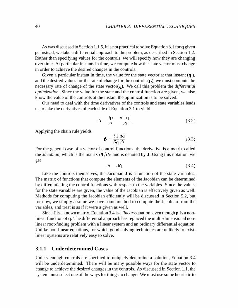
40 CHAPTER 3. DIFFERENTIAL TECHNIQUES
As was discussed in Section 1.1.5, it is not practical to solve Equation 3.1 forq givenp. Instead, we take a differential approach to the problem, asdescribed in Section 1.2.Rather than specifying values for the controls, we will specify how they are changingover time. At particular instants in time, we compute how thestate vector must changein order to achieve the desired changes in the controls.
Given a particular instant in time, the value for the state vector at that instant (q ),and the desired values for the rate of change for the controls( _p), we must compute thenecessary rate of change of the state vector(_
q). We call this problem thedifferentialoptimization. Since the value for the state and the control function are given, we alsoknow the value of the controls at the instant the optimization is to be solved.
Our need to deal with the time derivatives of the controls andstate variables leadsus to take the derivatives of each side of Equation 3.1 to yield
_p =
dp
dt
=
df(q)
dt
: (3:2)
Applying the chain rule yields
_p =
@f
@q
dq
dt
: (3:3)
For the general case of a vector of control functions, the derivative is a matrix calledtheJacobian,which is the matrix@f=@q and is denoted byJ: Using this notation, weget
_p = J _q: (3:4)
Like the controls themselves, the JacobianJ is a function of the state variables.The matrix of functions that compute the elements of the Jacobian can be determinedby differentiating the control functions with respect to the variables. Since the valuesfor the state variables are given, the value of the Jacobian is effectively given as well.Methods for computing the Jacobian efficiently will be discussed in Section 5.2, butfor now, we simply assume we have some method to compute the Jacobian from thevariables, and treat is as if it were a given as well.
SinceJ is a known matrix, Equation 3.4 is alinearequation, even thoughp is a non-linear function ofq. The differential approach has replaced the multi-dimensional non-linear root-finding problem with a linear system and an ordinary differential equation.Unlike non-linear equations, for which good solving techniques are unlikely to exist,linear systems are relatively easy to solve.
3.1.1 Underdetermined Cases
Unless enough controls are specified to uniquely determine asolution, Equation 3.4will be underdetermined. There will be many possible ways for the state vector tochange to achieve the desired changes in the controls. As discussed in Section 1.1, thesystem must select one of the ways for things to change. We must use some heuristic to

3.2. SOLVING THE DIFFERENTIAL OPTIMIZATION 41
pick a solution, because we lack any information as to what isdesired. The rule chosenfor the differential approach is to minimize the amount thatthe configuration changes,or, more precisely, to minimize the rate of change of the configuration. That is, if theuser’s controls don’t ask for something to change, the system should avoid changing it.This leaves open a variety of ways to measure change that willbe explored in Section3.4. Since the rate of change of the configuration will be a linear function of the rateof change of the variables, its magnitude will be a quadraticfunction, which we denoteby g:
When the linear system of Equation 3.4 does not uniquely determine _q , it provides
constraints on its possible value. To determine the particular value of _q, we must solvethe problem
minimize E = g(_q) subject to _p = J
_q: (3:5)
That is, we have cast the problem as a constrained optimization: minimize the value ofa quadratic objective function of_q, subject to the linear constraints that the controls aremet. In the following sections, we discuss solution methodsusing standard techniquesthat meet the needs of differential manipulation.
3.2 Solving the Differential Optimization
The linear/quadratic constrained optimization problems are a standard class of prob-lems for which a wide range of techniques have been developed. Good surveys can befound in texts such as [Fle87] and [GMW81]. A standard technique is the Lagrangemultiplier method. A form of it is reviewed here for use in thedifferential approach.
To begin, we consider minimizing a specific quadratic objective function, simplyminimizing one half the magnitude of_q squared. The value of_q that minimizes that isthe same value that minimizes the magnitude of_
q. The specific constrained optimiza-tion problem we consider in this section is then
minimizeE =
1
2
( _q � _q) subject to _p = J _q: (3:6)
We will consider the general case of quadratic objectives inSection 3.4.To provide an intuition for how Lagrange multiplier methodswork, consider an ex-
tremely simple case: a particle in 2 dimensions, with its state represented as its Carte-sian coordinates,q � fx; yg: We will place a control on the particle that is its distanceto the origin,p = f(q) = x
2
+ y
2
: Suppose we specify_p to be 1.As shown in Figure 3.1, there are many possible values for_
q which achieve thedesired value for_p: In this case, it is clear to see that the one with smallest magnitudeis the one which is in the same direction as the gradient off: Any component of_q notalong this line will not be helping to achieve the desired controls. We can thereforerestrict _q to be some multiple of the gradient, that is,_
q can be expressed as a scalingfactor times the gradient. This scaling factor is called theLagrange Multiplier.

42 CHAPTER 3. DIFFERENTIAL TECHNIQUES
f
Figure 3.1: A point on the plane with a radial control. Many possible values of _q will yieldthe desired value of_p: The one with least magnitude has the same direction as the gradient off:
If there were multiple controls, each would make a contribution to _q. For each
control, the contribution is some multiple of its gradient.We therefore have a vector ofLagrange multipliers, which we denote by�: _q is determined by the linear combinationJT�:
More formally, to be a solution to the constrained minimization problem, _q mustsatisfy two criteria. First,_q must satisfy the linear constraints, given by Equation 3.4.Secondly,_qmust minimizeE as much as possible, subject to the constraints. In the caseof an unconstrained minimization, we would require that thegradient@E=@
_q vanish,
meaning that there is no direction to change_q that would result in a lesser value for
E: With constraints, there might be a way to change_q to further minimizeE; but
only if these changes are prohibited by the constraints. That is, if the gradient of theobjective function is not zero, it must lie in the row space ofthe constraint gradients.This requirement is expressed by defining the objective function gradient to be a linearcombination of the constraint gradients,
@E
@_q
= J
T
�; (3:7)
for some value of�: The vector� is an intermediate result which we call theLagrangemultipliers.
In the case of the simple objective function of Equation 3.6,the gradient@E=@_q is
simply _q, giving
_q = J
T
�: (3:8)
Substituting this into Equation 3.4, gives
_p = JJ
T
�; (3:9)
a linear system which can be solved for its one unknown,�: This intermediate resultcan be substituted back into Equation 3.8 to yield the desired final result,_q.

3.2. SOLVING THE DIFFERENTIAL OPTIMIZATION 43
3.2.1 Over-determined Cases
To this point, we have focussed on techniques that handle thecases where an insufficientset of controls are specified to uniquely determine a solution. We now must considerthe problem of handling cases where too many controls specify the solution. Such casesmay involve redundant controls, where multiple controls all specify the same solution,or conflicts, where there are no solutions to all of the controls.
Conflicting controls are obviously a problem as there is no solution which will meetthe controls. However, redundant controls manifest themselves in exactly the sameway. Consider a system subject to two identical controlsp
1
andp2
: The net resultshould be that_q moves in the manner specified. But_q is created by the sum of thecontributions ofp
1
andp2
: How much does each contribute? Doesp
1
contribute a littleandp
2
a lot? Doesp1
contribute a huge positive amount andp
2
a huge negative amount?When controls are over-specified, whether their values conflict or not, they cause the
Lagrange multipliers to be under-specified. The matrixJJT will be singular. Redundantor conflicting controls are inevitable, and are notoriouslyhard to detect. It is importantthat our solution method be robust in the face of these singularities, and that it will dosomething reasonable with conflicts.
One approach to handling the over-constrained cases would be to employ a linearsystem solver which could handle Equation 3.9 even when the matrix is singular. Forexample, singular value decomposition (SVD) [PFTV86] could be used. The SVD hasmany attractive properties, for example it provides information as to which controls areredundant. Unfortunately, SVD is expensive to compute. In contrast, if we can restrictthe problem so that the solver only needs to solve non-singular systems, we can exploitthis property to solve them efficiently, as will be discussedin Chapter 4.
Rather than force the solver to handle singular matrices, wewill instead modifythe matrices so that they have a unique solution. We will not get an exact solution tothe original linear system, but we are trading accuracy for improved behavior in badcases. Because we are interested in interaction, rather than high accuracy quantitativemethods, we will make such tradeoffs often, as discussed further in Section 4.5.
The technique for making the matrices non-singular is called damping.The basicintuition is that we generally prefer to avoid large values for the Lagrange multipliers,therefore, in cases where the Lagrange multipliers are undetermined, we should min-imize their magnitude. The derivation here most closely follows that of Nakamura’sderivation of a robust pseudo-inverse [Nak91].
In cases where the controls are over-determined, the solverwill not be able toachieve all the desired values for them. Instead, we must settle for getting as closeas possible, that is, to satisfy them in a least squares sense. To find Lagrange multipli-ers that achieve this minimum, we minimize1=2(JT
� � _q) � (J
T
� � _q); In addition,we would like to minimize the magnitude of�; although since this is not as important,we can scale this term by a small amount, which we will call�: The function we wish

44 CHAPTER 3. DIFFERENTIAL TECHNIQUES
to minimize is
E =
1
2
(J
T
�� _q) � (J
T
�� _q) + �(� � �): (3:10)
The minimum of this quadratic is found by differentiating with respect to�; and settingthat equal to 0, yielding
0 = JJ
T
�� J _q + �I�; (3:11)
whereI is the identity matrix. Recalling Equation 3.4, a little rearrangement yields
_p = (JJ
T
+ �I)�; (3:12)
a variant of Equation 3.9 which has small amounts added to thediagonal of the matrix.Rather than having a single scaling factor for the magnitudeof the vector of La-
grange multipliers, we could have an individual one for eachindividual multiplier. Thiswould enable damping selectively, or to damp some controls more than others. Selec-tive damping allows the creation a a limited constraint hierarchy: if two constraintsconflict, and one is damped but the other is not, the undamped constraint will domi-nate the damped one. When two conflicting controls are both damped, their effects areblended. By individually adjusting their damping values, the controls can be weighted.The larger the damping value, the less weight the control receives.
The damping technique presented here has three major drawbacks. First, it penal-izes large values of the multipliers whether they are underdetermined or not. This cancause a problem when the multipliers legitimately need to belarge to satisfy the desiredcontrols. Secondly, damping is applied whether there are conflicting controls or not.Finally, it introduces a new dimensionless parameter�: Because it has no real mean-ing to the original problem, values for it are difficult to determine. For the differentialapproach, damping values must be determined empirically.
3.3 Solving the Differential Equation
The methods of the previous section permit us to compute the rates of change of thestate vector. We now consider how to use the rates to find the trajectories of the con-figurations over time. We must solve the problem of computingthe trajectory of thestate given its initial value and time derivatives, a problem of solving an ordinary dif-ferential equation (ODE) from an initial boundary condition. Here, we provide a briefintroduction to handling this problem in the context of the differential approach. For amore complete, but still practical, introduction to ODE solution methods, see Chapter15 of [PFTV86].
The value ofq is actually is a function of time, defined by a function that computesits time derivative. The form that we have this function defined in is
_q = f
0
(q; t); (3:13)

3.3. SOLVING THE DIFFERENTIAL EQUATION 45
wheref0 is found by solving the differential optimization. Given the value forq (whichcorresponds toq(t) for some timet), we can compute_q . This is a standard form foran ODE.
For the types of problems we encounter with the differentialapproach, we cannotsolve the ODE in closed form. Instead, we must solve it numerically by discretizingtime into a series of small steps. In computing a step, the following problem must besolved: given the state at the current time,q(t), find the state at some time in the future,q(t+�t): The time derivative_q (i.e. the result of the differential optimization) does notdirectly provide the solution to this problem. It only specifies how the state is changingat the instant that it is computed. The problem of updating the state given the abilityto find its time derivatives is solving an ordinary differential equation from an initialboundary condition.
Solving the ODE is difficult because when we perform an evaluation to find _q for
a particularq , we are only finding out about a particular instant in time . Wehave noinformation about the future._q might remain constant for the duration of the step, butit might also change drastically over the course of the step.
The simplest method for solving an ODE is to find_q at the beginning of the stepand assume it remains constant over the course of the step. This is known as Euler’sMethod, and has the simple update rule of
q(t +�t) = q(t) + �t _q(t): (3:14)
Euler’s method approximatesq(t) with as a piecewise linear function. The size of eachpiece is the step size. If the step is too large, the approximation will not be good. Noticethat each step requires computing a new_q by solving the differential optimization.
To understand what is meant by “good” in ODE solving within the context of thedifferential approach, consider a simple example. Once again, we will use a point inthe plane, however, this time, we will select a control that is its angular position aboutthe origin. Suppose we provide a desired velocity for this control of 1 unit per unittime, the starting configuration has the point a unit distance from the origin along thepositivex axis, and the specified derivative always points tangent to the circle. As timeprogresses, we will expect the point to move around the origin in a circular path.
If an Euler’s method ODE solver is applied to this example, the problems of ODEsolving are quickly apparent. At the initial position on thex axis, the gradient of thecontrol points vertically. Any step in this direction will lead the point off the circle it isexpected to follow around. As more and more steps are taken, the point will continueto spiral away from the circle, speeding off the page, as shown in Figure 3.2.
Because of error in approximation, the point spirals outward over time. However,if smaller step sizes are taken, the behavior is better. Thatis, the point spirals outwardmore slowly, better approximating the expected circle. This is shown in Figure 3.3. Infact, by going more slowly, we may reach a desired destination more quickly becausewe are less likely to overshoot or drift away from the target.Going slowly can be

46 CHAPTER 3. DIFFERENTIAL TECHNIQUES
Figure 3.2: A point on the plane with a control that drives it tangent to a circle around theorigin. Although it should (ideally) travel in a circular path, ODE solver error causes it to spiraloff the page.
Figure 3.3: A point is pushed in a direction tangent to a circle about the origin, using an EulerODE solver and various step sizes. In all cases, the point spirals away from the target circle,although with small step sizes, the point tracks the circle better.
accomplished two ways, either by reducing the duration of the step or by reducing thevelocities.
In solving the ODE, there is effectively a speed limit. If an object attempts to changefaster than this, it may speed out of control or even miss its destination entirely. Fora given velocity, solving can be made more stable by reducingthe step size, in thelimit of infinitesimally small step sizes, ODE solving will be exactly correct. However,since each step may require significant computation, the number that can be executedis limited. Alternatively, this speed limit can be viewed with a constant step size: fora given step size, how fast can an object go without becoming unstable. If we thinkof steps as taking some fixed amount of time to compute, this translates directly to anapparent velocity in the image.
The speed limit given by ODE solving varies according to a number of factors.Most significantly, it depends on the path that the objects take. The more non-linearthe function is, the more poorly the linear approximation will fit it. At the extreme,if an object is truly moving in a line, Euler’s method achieves the exact motion, andthere is no speed limit. In a sense, the speed limit can be viewed as a restriction on thetypes of controls used to define the motion: given that the step size is fixed, how badlynon-linear a control can be used and still have the object move at a reasonable rate.

3.3. SOLVING THE DIFFERENTIAL EQUATION 47
If we take smaller steps to achieve better performance, we might use multiple ODEsolver steps for each redraw. For example, if we would like tomaintain 10 frames persecond and updating the image or solving the differential optimization takes 30ms, wemight use two Euler steps between redraws. As we will see in Chapter 4, typically thedifferential optimization is the most time consuming part of the process, and becomesmore so as the problems grow larger. With a faster computer, the time to compute eachstep will be decreased, so more steps can be computed per redraw, effectively raisingthe speed limit.
Using multiple samples per step is what is calledmulti-step solving.We mightphrase the problem as follows: the starting point (t andq(t)), computeq(t + �t) aswell as possible usingn samples. Using two Euler steps hasn = 2; and uses a 2 piecepiecewise linear approximation.
Given that we have some number of samples that we can make in a step, we canconsider how to best use these samples to approximateq(t): For example, if we cantake 2 samples, we might use a 2 piece linear approximation bytaking two Euler steps.Alternatively, we might use these same two samples to fit a parabola. This would becalled a2nd-ordermethod. The particular case of a parabola is simple to create, sincea parabola has a linear function for its derivative. This is effectively done by using theinitial step as a trial step, evaluating the derivative at this point, and using this for theduration of the step. This is called themidpoint methodor the 2nd-order Runge-Kuttamethod. It is applied to the example problem in Figure 3.4.
According to Press et al.[PFTV86], the most popular multi-step method is the 4th-order Runge-Kutta method. As implied by the name, it uses 4 evaluations per step.According to the literature, this method is generally perceived to be superior to higherorder methods. The 4th order Runge Kutta method has been the preferred solver forthe prototype implementations in this thesis.
A higher order method is only better than taking a larger number of lower ordersteps if it provides a higher speed limit for the same number of evaluations. This will, ofcourse, depend on the problem to be solved. However, in practice, the 4th-order Runge-Kutta method seems to be a good method for implementing the differential approach.Empirically, it usually performs at least as well, but sometimes substantially better, thantaking 4 small Euler steps, or 2 Runge-Kutta 2 steps.
There are many other multi-step methods. Predictor-Corrector techniques [PFTV86]are another popular strategy. Such methods use past steps topredict future values andthen correct for the error of the prediction. However, thesemethods are difficult toapply in dynamic settings because the dynamic nature of the problems make it diffi-cult to maintain a history to use in prediction. Often, therewill be no history so sometechnique like Runge-Kutta will be needed to start the process.
For the prototype implementations of this thesis, fourth order Runge-Kutta and Eu-ler’s methods solvers are used.

48 CHAPTER 3. DIFFERENTIAL TECHNIQUES
Figure 3.4: Left, a second order Runge-Kutta method, and right, an Euler’s method are usedin the example problem of Figure 3.2. The evaluations used bythe Runge-Kutta solver areshown in grey. Notice how the Runge-Kutta solver stays closer to the circle using the samenumber of evaluations as the Euler solver.
3.3.1 Adaptive Step-Sizes
So far, we have considered solving an ODE with fixed step sizes. Instead, we mightconsider adapting the step size to the problem. When a step is made, it could be checkedto see how good it was. If it caused an unacceptably large amount of error, it could beredone with a smaller step size. Adaptive step size methods have the advantage thatthey can slow down to accurately handle problems when they become difficult. Also,because they check their results, they are less likely to cause bad errors.
Adaptive step size methods have some severe drawbacks when used with the dif-ferential approach. The most significant problem is that they are continually adjustingthe step size which alters the amount of computation required to advance simulationtime a specified amount. If the computation rates are fixed, the apparent velocities ofobjects will fluctuate. This can be disconcerting to the user. Also, the extra evaluationsto perform checks and computing alternate steps might be better spent on making moresteps since error correction is built into the controls, as controllers can adjust their val-ues in response to what is happening as will be discussed in Section 6.3. For example,in the example of the previous section, if the user really cared about the point stayingon the circle, an additional control that maintained this would be used.
The differential approach provides some interesting opportunities for employingadaptive step sizes. Standard methods for ODE solving treatthe equation as a black

3.4. GENERALIZED OBJECTIVE FUNCTIONS 49
box, that is they cannot get any information about the problem other than asking forevaluations of_q . Standard adaptive ODE solvers employ methods such as taking thesame step with a higher order method to compare with.
With the differential approach, we have more information about the problem weare solving. In particular, the functions that define the controls provide measures oferror. For example, if a controller is meant to keep a controlat a particular value, at theend of the step it can be checked to insure that the control hasnot changed too much.Each different control might have its own way of defining whatan acceptable amountof error is. I call thissemantic adaptationbecause it adapts based on the meaning ofthe problem. I have experimented with some simple semantic adaptation of step size,simply reducing the step size when a control has a value that the system finds unaccept-able. The method works as follows: a certain set of controls are monitored. When astep is computed, the monitored controls are examined. If any exceed a specified errorlimit, the step size is shortened.
A different type of semantic adaptation is to use a differentstep when problemsoccur. One useful variant of this is the cleanup step. In an application like constraint-based drawing or mechanism simulation, there is typically some small number of con-trols that cause motion and a potentially larger number thatrepresent constraints. Acleanup step is an extra step that is run only with the constraints. It is used when thepulling controls have broken the other constraints to causethem to get back to theirdesired configuration.
3.4 Generalized Objective Functions
The optimization objective determines which solution willbe given in under-determinedcases. By selecting different optimization objectives, different default behaviors canbe given to objects. To this point, we have only consider one optimization objective:one half the magnitude of the state vector derivative squared. This section considersother objective functions.
The types of default behavior that we consider in the Differential Approach can besummarized by the idea that objects should not change unlessa control causes them tochange, and that when an object changes to achieve what is specified by a control, itshould do so by changing as little as possible. By altering how we measure change, wecan control the default behavior or feel of an object. For an example, consider manip-ulating a line segment by moving one of its points, as shown inFigure 3.5. Dependingon the metric of change, the line segment will behave differently. In all cases, the linesegment achieves what is specified by the controls. However,by selecting an appro-priate metric, the programmer can create a desirable default behavior. An appropriatemetric is not essential since if there was something that wasimportant, it could be spec-ified with a control. But, properly defined objectives can alleviate the need for extra

50 CHAPTER 3. DIFFERENTIAL TECHNIQUES
(a) (b) (c)
Figure 3.5: A line segment is dragged by controls that specify the position of the upper point.Different objective functions provide different behaviors: a) change in length and orientationare minimized; b) change in the position of the center is minimized; c) change in the positionof the lower point is minimized.
specifications.The simplest metric of change is the magnitude of the rate of change of state vector,
_q, as was used in Section 3.2. This simple objective has been used up to this point, andis sufficient for a wide variety of applications. It has a drawback: it causes the param-eterization to affect the behavior of the object. Using the parameterization violates thegoal of separating manipulation from representation. Evensimple decisions, such aswhether to represent an angle by degrees or radians, can affect an object’s behavior[Wit89a]. This may be a serious problem, or an opportunity. It means that we canchoose which interactive behavior we would like by carefully choosing the representa-tion. However, if we are not careful about choosing the representation, we might get aless desirable behavior. The severity of this problem is limited, because the user couldalways provide additional controls if they really cared what happened.
3.4.1 The Metric
In order to spare the user the increased effort of more completely specifying their intent,and to give programmers more freedom to select representations that are convenient,we must use a different objective function. Rather than measuring change in values ofthe parameters, we could measure change in something that did not depend as closelyon the representation. We have used the functions that compute objects’ attributes toserve as controls that are independent of representation. Similarly, we prefer to definean object’s metric in terms of its attribute functions as well. We select a subset of theattributes to define the metric. Just as we denote the subset of the attributes that serveas the controls asf; we will denote the function used to define the metric byg which isalso a function ofq. We denote the Jacobian@g=@q by G:
The optimization objective will be to minimize the magnitude of the change in theattributes. This rate of change is
_g = G_q: (3:15)
Since we are searching for the minimum, we can minimize1=2 the sum of squares of

3.4. GENERALIZED OBJECTIVE FUNCTIONS 51
g; rather than the magnitude. Since we might wish to emphasize some of the attributesmore than others, we also introduce a scaling factor for eachto make the objective aweighted sum of squares. Writing the scaling factors as the diagonal elements of amatrix for notational convenience, the objective functionis
E =
1
2
_q
T
G
T
SG_q; (3:16)
We will call the matrix that defines this quadratic (GTSG) term themetricbecause itdefines a way to measure_q.
The simple objective function of Section 3.2 used the parameters of the objects asthe attributes that defined the metric. Sinceg = q; G = I andM also is the identitymatrix. Viewed this way, the advantage of using a correct metric can be seen. Theidentity metric defines the behavior of the object in terms ofits parameters, rather thanin terms of something that is potentially meaningful to the user.
A Particularly Useful Metric
The metric provides a method for an interface designer to define a default behavior foran object. In effect, it allows for hand-tuning the behaviorthat a user sees when the ob-ject is manipulated. However, this leaves the problem that the interface designer musthand-tune the behavior in order to hide effects of the parameterization. Often, this isnot an issue, as the parameters provide a reasonable defaultbehavior, or, if a specificbehavior is required, it can serve to describe a metric. However, some applicationsdemand an automatic method for determining a metric that provides a consistent, pa-rameterization independent, feel for a variety of objects.Such a method is particularlyuseful in cases where a user may define object behavior. An example is the parametriccurve manipulation of Section 8.1.1 and Section 9.4.
An analogy to physics provides an automatic, consistent metric for a broad class ofobjects. As first suggested by Witkin [Wit89b], we can imagine an object as a physi-cal entity with an uniform mass distribution. In effect, we can view each pixel of theobject as an atom, each with a tiny bit of mass. This mass distribution defines how theobject changes as forces are applied in particular places. Inertia causes each particle tomove as little as possible. The mass distribution serves as the metric does, defining thebehavior of objects in response to controls. Witkin and Welch [WW90] used specifi-cation of the mass distribution to allow animators to specify the the default behaviorsof simulated objects that were acted upon by point controls.
When solving the equations of motion of a physical object in generalized coordi-nates in order to simulate it, the mass distribution is encoded into a matrix known asthe inertia tensor or mass matrix [Gol80]. This matrix is found by accounting for theeffects of each particle on the objects’ behavior by integrating over the mass distribu-tion. When such a matrix is determined numerically, the integral is approximated bysampling a set of particles.

52 CHAPTER 3. DIFFERENTIAL TECHNIQUES
Analogously, a metric can be defined by viewing a graphical object as a collectionof “particles” and minimizing the motion of these particles. In practice, the distributionis estimated by a set of points. We define the metric functionsto be the positions ofan evenly spaced set of points on the object. We call such a metric the mass matrixbecause of its physical analog.
The mass matrix is an important metric because it can be defined independentlyof the object. For any graphical object, a set of points can beevenly distributed eitheralong its length (for a curve) or within its area (if it is solid). Section 8.1.1 will illustratethe utility of this, allowing default behavior to be automatically provided for a widevariety of objects.
3.4.2 Solving the Generalized Quadratic Objective
Using a different quadratic optimization objective requires a slightly different set ofmethods for solving the constrained optimization problems. In this section, we derivethe method in its full generality for the case of any quadratic objective function andlinear constraints.
The standard form of a vector quadratic equation is
E =
1
2
x
T
Mx+ b
T
x+ k; (3:17)
wherex is the vector parameter (_q for this chapter),M is the quadratic or matrix term,the vectorb is the linear term, andk is a scalar constant. Since we are not interestedin the value itself, but rather only the value ofx that minimizes it, we can ignore theconstant as it goes away when we take the gradient, and we can multiply the quadraticby 1=2 as it cancels out other values later, simplifying the equations. The linear termpermits measuring change from a point other than 0, and will be used in Section 3.5.The methods of Section 3.2 solve the special case of this objective with an identitymatrix forM ; and 0 for the linear componentb:
The Lagrange multiplier derivation can again be applied, this time to Equation 3.17.We denote the linear constraints asAx = a: We require the gradient of the objectivefunction to be a linear combination of the of the constraints,
@E
@x
= Mx + bx = A
T
�: (3:18)
Solving this forx and denoting the inverse of the metricM�1 by W; gives
x =WA
T
��Wb: (3:19)
Inserting this into the constraint equationAx = a gives
AWA
T
� = a +AWb; (3:20)

3.4. GENERALIZED OBJECTIVE FUNCTIONS 53
a linear system that can be solved for�: Once� is computed, it can be inserted intoEquation 3.19 to computex:
The damping techniques of Section 3.2.1 are not taken into account by the gener-alized quadratic objective. Using a derivation similar to that of Equation 3.12, yields
(AWA
T
+ �I)� = a+AWb: (3:21)
Using the notation of the rest of the chapter,M is the metric as defined in Section3.4.1 and the linear constraints are given by Equation 3.4 soA = J anda =
_p:
3.4.3 An Approximation to the Metric
Using the metric to define the default behavior of an object has several advantages. Itpermits separation of manipulation and representation, and provides an abstraction fordefining the feel of an object. However, it has a significant cost: we must find the metricand invert it. This is problematic because the metric is large. Inverting a matrix thislarge would be prohibitive. One advantage to using the identity matrix as the metric isthat it is trivial to invert.
What we aim for in this section is an approximation to the metric that is inexpensiveto invert, yet provides some of the features of the full metric. The approximation weconsider is simply using the diagonal elements of the metric. This diagonal matrix istrivial to invert — we merely take the reciprocal of all its elements — and cheap to usein solving Equation 3.20. It still addresses some of the important issues that the fullmetric addresses, particularly the selection of units.
Consider again the example of dragging a line segment in Figure 3.5. Suppose itsconfiguration is represented by the position of its center, its length and its orientation,and that the simple identity metric objective function is used. If the upper left cornerof the segment is move a quarter of an inch to the left, the linesegment might have itscenter move, scale and rotate, or some combination of the two. Suppose that the posi-tion of the center of the line segment was represented in micrometers from the cornerof the page, the orientation represented as radians from horizontal, and the length ininches. To achieve the movement of the upper left point by simply moving the centerwould require the parameters to change very quickly as thereare many micrometersto be covered, while achieving the movement by scaling and rotating would requireconsiderably smaller changes in the parameters. Because the simple optimization ob-jective minimizes change in the parameters, the latter would be chosen. If the positionof the center were measured in miles instead, a very tiny change in the position of thecenter would create the needed motion, so this would be selected by the optimizationcriteria.
In the example, the simple selection of units with which to represent the positionof the center of the line segment determined the dragging behavior. The problem is

54 CHAPTER 3. DIFFERENTIAL TECHNIQUES
parameters having different units. One way around this is todefine an objective func-tion which minimized the amount of change in the parameters after converting them tosome standardized units. Suppose we knew the conversion factors between the unitsof the parameters and the standard units. We would have a scaling factor for each pa-rameter. For notational convenience, we can write the scaling factors as the diagonalelements of a diagonal matrixS; so the component-wise scaling of parameters wouldsimply be the multiplicationSq:
Rather than simply minimizing the magnitude of_q, we would instead minimize the
time derivative of the scaled parameters,S_q; giving
E =
1
2
(S _q � S _q); (3:22)
or, to use the generalized notation of Equation 3.17
M = S
T
S: (3:23)
We see that we have a diagonal metric.The problem is to determineS to convert the parameters to the standard units. One
way to define standard units would be to require that equal changes in each variableshould affect the attributes the same amount. As for the metric, we pick a subset ofthe attributes to define the objective function, and denote the function that computesthese attributes byg: However, we are only interested in the derivatives with respectto a single variable at a time. That is we want to measure the change in all of theattributes ofg with respect to each variable independently. For a particular variable,the scaling factor is the magnitude of the derivatives of each element ofg with respectto the variable, that is,
S
ii
=
s
g
q
i
�
g
q
i
: (3:24)
The diagonal terms in Equation 3.23 are the scaling factors squared,
M
ii
=
g
q
i
�
g
q
i
: (3:25)
These are exactly the diagonal terms of the metric in Equation 3.16.The diagonal metric cannot take into account interactions between variables. While
it can remove differences in units between similar terms, itcannot make two differentrepresentations seem alike. In the line segment example, iteliminates the effects of thechoice of units, however it does not remove the effect of a completely different param-eterization. It could not, for example, express an objective function that minimized themotion of the endpoints. Therefore, no matter what diagonalmetric are chosen, a linesegment parameterized by position of center, length and orientation will feel differentthan a line segment parameterized by the positions of its endpoints.

3.5. SOFT CONTROLS 55
3.5 Soft Controls
The generalized objective functions of the last section allow the creation of objectivefunctions that can be used to control the object. To this point, we have discussed de-fault behaviors for objects that causes objects to minimizes their motion if controls arecausing them to change, they do not change. In this section weconsider an alternative:having objects change by default unless a control specifies otherwise. The non-zerodefaults lead to linear terms in the general quadratic optimization objective functionof Equation 3.17. Using this term will enable soft controls:controls which are over-ridden by the regular controls. These are important becausethey allow us to createbehaviors such as dragging subject to constraints, where anobject is manipulated bythe user but constraints will not be violated. While these techniques do not providegeneral constraint hierarchies as described by Borning et al.[BFBW92], the draggingsubject to constraints that they can provide is useful in many graphical applications.The use of optimization objective terms to provide user control was pioneered in thevision research of Kass et al.[KWT88].
Suppose that we had some desired default value for_q, denoted_q
0
. Rather thansimply minimize the magnitude of_q, we would instead minimize its difference fromthe default value, so
E =
1
2
(_q�
_q
0
) � (_q�
_q
0
): (3:26)
In terms of the generalized objective function of Equation 3.17, the coefficients of thelinear termb in this case is_q
0
. Similar metrics can be worked out to include a metricas well. While the generalized solution of Section 3.4.2 can be applied, we review thederivation for this important special case here as it provides insight.
To provide intuition for how this works, consider again the simple point examplefrom Section 4.3. Notice that the control specifies the behavior only in the direction ofits gradient, so the optimization objective is free to do whatever it wants in an orthog-onal direction. Suppose that we have specified_p to be 0. This restricts_q to lie alongthe line perpendicular to the gradient, as shown in Figure 3.6. To find _
q closest to_q0
,we must project_q
0
onto this line. We do this by adding in a component of_q which
cancels out the disallowed portion. Thisconstraint componentmust be a multiple ofthe gradient. This multiple is the Lagrange multiplier.
We compute_q as the sum of two components, its default value_q
0
and the contri-butions of the controls,_q
c
; so_q = _q
0
+ _q
c
: (3:27)
Since _q must satisfy the controls, we substitute this into Equation3.4, to yield
_p = J( _q
0
+ _q
c
): (3:28)
Since the contribution of the constraints is a linear combination of the control gradients,

56 CHAPTER 3. DIFFERENTIAL TECHNIQUES
q0.
qc.
q.
Figure 3.6: A hard controls constrains the distance from the point to theorigin. Any move-ment of the point must be orthogonal to the gradient of this control. When a default velocity( _q0) is given for _q, it must be projected into the space that meets this restriction. To achievethis, a component is added to_q
0
that projects it onto the space where_p = 0:
we define the Lagrange multipliers as
_q
c
= J
T
�: (3:29)
Which, with a little rearrangement yields
_p� J _q
0
= JJ
T
�; (3:30)
a linear system, which like Equation 3.9 can be solved for�; which in turn determines_q
c
by Equation 3.29, from which_q can be computed by Equation 3.27. Notice thatwhen _q
0
= 0; the method of this section is exactly the same as that of Section 4.3. Thedamping techniques of Section 3.2.1 also apply.
3.5.1 Determining the Values for Soft Controls
We now must figure out how to obtain_q0
. Our goal is to provide soft controls that workas the hard controls do, except that the hard controls are given precedence over them.Soft controls are defined asps = fs(q); but like the hard controls, would be specifiedby their derivatives,_p
s
:
If the soft controls do not conflict with the hard controls, they can simply be treatedas hard controls. The more interesting cases, however, are when the hard controls limitthe soft controls. The ultimate goal is to have have soft controls work exactly as hardcontrols do, except in the cases where there are hard controls that take precedence overthe soft controls.
We would like to satisfy the soft controls as closely as possible subject to the restric-tion that the hard controls are specified exactly. We can define the objective functionto minimize the squared error of the soft controls meeting their desired values
minimize E =
1
2
(J
s
_q� _p
s
) � (J
s
_q� _p
s
) subject to _p = J _q: (3:31)

3.5. SOFT CONTROLS 57
p=x2-x1p=0. ps=x2
ps=1.
Figure 3.7: Two points are connected by a hard control constraining their distance. Theright point is also pulled by a soft control. If the soft controls are computed independently, anon-optimal solution may be found, as shown on the left. The soft control may specify thatthe right point should move, but part of this motion might be removed by the constraints. Asshown on the right, there is a solution that both satisfied theconstraints and meets the desiredvalues for the soft controls.
Such an objective function is the similar to the definition ofthe metric in Section 3.4.1,except that rather than minimizing the magnitude squared ofthe change of the deriva-tives of the functions value, we minimize the magnitude squared of the difference be-tween the derivative’s value and a default value. Generalized sets of soft controls (e.g.Js) will lead to M terms in Equation 3.17. The problems in using general metrics alsoapply to soft controls: A sufficient number of soft controls must be specified to uniquelydetermine_q in all cases, even when there are no hard controls. If an insufficient numberof soft controls are specified,M will be singular. Problems with ill-conditioning andefficiency in invertingM make this soft control scheme impractical. In this section,weconcentrate on methods for simpler achieving soft controlsby computing values for_q
0
.
Two-Pass Solver
One way to find_q0
is to ignore the hard controls, and simply use the method usedforhard controls for the soft controls. Using this approach, two linear systems are solved:first, a linear system is solved to compute the Lagrange multipliers that will determine_q
0
, then a linear system is solved to project_q
0
into the subspace allowed by the hardconstraints.
The method of computing the soft controls independently hasa serious drawback: itdoes not achieve the desired solution. Consider a case wheretwo points are connectedwith a hard control constraining their distance, and a soft control pulling one of thepoints to the right, depicted in Figure 3.7. The soft controlalone would move one ofthe points, violating the hard control. When this is projected into the legal subspace,part of the motion world be cancelled out. However, if all thecontrols were treatedequally, the other point could be moved to satisfy the hard control.
An alternative is to account for the hard controls in computing _q
0
. We compute_q0
using the methods we would use for the hard controls, except that we include both thehard controls and the soft controls in the computation. Damping must be used in case

58 CHAPTER 3. DIFFERENTIAL TECHNIQUES
the controls conflict. We then solve an optimization problemagain using the result ofthe first solution as_q
0
, and just using the hard controls as constraints. I first usedthistechnique in theBriar drawing program described in Section 9.1, and therefore call ittheBriar-style solver.
In cases where all the controls, both soft and hard, are consistent, theBriar-stylesolver has the nice property that both hard and soft controlsbehave the same. It isalso the case that the effort in solving the linear system twice can be avoided by firstchecking to see ifJ _q
0
= _p; in which case_qc
will trivially be 0. When using an iterativelinear system solver, as described in Section 4.3.1, this check happens automatically.
However, if we knew that the hard and soft controls did not conflict, then therewould be no need to have soft controls. In the cases where there are conflicts, theBriar-style solver has a few drawbacks. Most obvious is that it requires solving thelinear system twice, which can be expensive. Also, since solving the larger system willhave conflicting constraints, damping must be used. The solver does not actually solveEquation 3.31, but instead minimizes the difference between the damped result, whichalready partially accounts for the hard constraints.
Spring Controls
An alternate method to compute_q0
is to use gradient descent to drive the soft controlsto their desired values. We compute_q
0
to have the direction of the gradient of the softcontrol functions, and a magnitude proportional to how far from the target it is,
_q
0
= kJ
s
(p
s
� f
s
(q)); (3:32)
wherek is a scaling constant. This causes the controls to be pulled towards their desiredvalues with a decaying attraction: as the control nears its desired value, the rate at whichit is being pulled is decreased. In the physical analogy of Section 1.2.2, this attractionis a spring. Equation 3.32 is the generalized force version of Hooke’s law.
I will call these spring-like controlsspring controlsor simplysprings.Their methodcan be viewed as a cheap way to estimate the Lagrange Multiplier, an attempt to use gra-dient descent to achieve desired values for the soft controls, or as generalized springs,if we view the optimization as a physical simulation. Despite the fact that they are alittle harder to justify, they do work very well.
3.6 An Alternate Technique
The methods presented in the last sections described Lagrange multiplier techniquesfor solving constrained optimization problems with linearconstraints and a quadraticobjective function. The methods build a linear system and solve for an intermediateresult, the Lagrange multipliers. The methods have the advantage that they permit theuse of any quadratic objective function.

3.6. AN ALTERNATE TECHNIQUE 59
Often, we do not exploit generality of the Lagrange multiplier formulation. Forexample, the simple objective functions of Equation 3.6 or Equation 3.26 may be suf-ficient. In such cases, alternate, special purpose solutionmethods are sufficient.
The objective function that simply minimizes the magnitudeof _q gives an importantspecial case called a linear least squares problem. This is avery standard problem innumerical analysis. Example solving methods include singular value decomposition(SVD), QR factorization, and pseudo-inverses. These methods, and many others, arediscussed in [GL89]. Unfortunately, these methods are almost all extremely expensiveto compute, as they are unable to exploit properties of the problems such as sparsitythat we will use in the next chapter to speed performance.
Iterative solvers may also be used to solve the linear least squares problem. Inparticular, conjugate-gradient solvers, discussed in Section 4.3.1, are relevant to im-plementing the differential approach. Variants of conjugate-gradient find a solution tothe linear system, but have the property that the solution they provide to a linear sys-tem is solution closest to the starting point. Therefore, ifthe solver is begun with azero starting point, the solution with least magnitude is found. The conjugate-gradientlinear system solver in the Numerical Recipes text [PFTV86]is such a solver. To im-plement soft controls using the conjugate-gradient, Equation 3.28 is solved for_q
c
usingthe conjugate-gradient solver.
Using a least squares solver to implement the differential approach effectively solvesEquation 3.4 directly, without first computing the Lagrangemultipliers. For instance,implementing the differential approach by using a conjugate gradient algorithm worksvery well. The solver given in the text of Press et al.[PFTV86] permits the two mostoften used objective functions, and handles over-determined cases by providing a min-imum norm residual solution to the linear system. Using the algorithm is a very practi-cal way to implement the differential approach. It performsextremely well in practice.This method served as the backbone of my early implementations, and is available bya run-time switch even in my most current versions.
The obvious question is why bother developing a more complextechnique whenthe simpler approach works so well. The three main reasons for using the Lagrangemultiplier techniques in this chapter over the simpler “direct” approaches such as usingconjugate-gradient are: the intermediate result of the Lagrange multiplier techniques(the Lagrange multipliers) will be useful in certain interaction techniques such as theactive set methods of Section 6.4; they place few restrictions on the linear system solverthat is used, so that fast algorithms can be found; and, they extend to other quadraticobjective functions. However, in cases where these advantages are not required, thesimpler approach is worth considering. The approach handles the two most often usedobjective functions, those of Equation 3.6 and Equation 3.26, so it is often sufficient.

60 CHAPTER 3. DIFFERENTIAL TECHNIQUES
3.7 A Concrete Example
To review the basic techniques of this chapter, we now consider a complete example indetail. Our object will be a fixed length line segment with a unit radius, represented bythe position of its center and its orientation. The control we will create is the positionof its endpoint. The state variables areq = fq
cx
;q
cy
;q
theta
g; and the controls arep = fp
x
;p
y
g.The control functions are:
p
x
= f
x
(q) = q
cx
+ cosq�
(3.33)
p
y
= f
y
(q) = q
cy
+ sinq�
:
The core of the implementation will be the differential optimization that will com-pute a value for_q given a value forq and _
p . This routine must first compute theJacobian of the controls,J, as a function ofq :
J =
"
1 0 � sinq�
0 1 + cosq�
#
: (3:34)
It then can compute values for the Lagrange multipliers by solving the linear system
_p = JJ
T
� (3:35)
for �; and then computing_q as_q = J
T
�: (3:36)
Suppose at the current time, the line was at a 45 degree angle with its center at theorigin (q = [0; 0; �=4]), and that the control specifies the endpoint to move right withunit velocity (_p = [1; 0]). The Jacobian of the controls is then
J =
"
1 0 �:707
0 1 :707
#
: (3:37)
To compute the_q, we must first solve the linear system"
1:5 �0:5
�0:5 1:5
#
� =
"
1
0
#
; (3:38)
then use Equation 3.36 to determine_q. At this particular instant,� = [:75 :25]; so_q = [:75 :25 � :35]. If we were to use an Euler step with step size .1, the configurationat the end of the step would beq = [:075 :025 :75]:
The basic control for interaction will be to repeatedly takeODE solver steps, inter-leaving redraw between the steps to give the illusion of motion. This solver will call thedifferential optimization routine, possibly several times per iteration. The ODE solver

3.8. SUMMARY 61
will also have to provide values for_p to the optimization routine. These values are whataccounts for the user’s motions; for example, they might be tied to the input device.Methods for determining desired velocities will be discussed in Section 6.3, however,one simple way of getting_p from the input device is to use decaying attraction: wecompute the vector from the position of the control to the pointer, and use a multipleof this for _p.
In this example, we are already using multiple controls, onefor each axis. Evenmore controls could be added. For example, suppose we wantedto add two morecontrols that position the other end of the line segment. These controls are computedby
p
x2
= f
x
(q) = q
cx
� cosq�
(3.39)
p
y2
= f
y
(q) = q
cy
� sinq�
:
The Jacobian would now be a 4 by 3 matrix.Since we most likely will not have two mice, rather than permitting the user to
control the position of the second point, we might want to constrain it to remain at theorigin. This would require specifyingp
x2
andpy2
to have values that caused the pointto move towards the origin, e.g. to be a negatively scaled multiple of the position of thepoint.
Clearly, these controls will conflict: the mouse might attempt to pull the other end-point away from the origin. This will cause the matrixJJT to be singular. In orderto solve the linear system, we might add damping by adding a small amount to thediagonal elements of the 4 by 4 matrix.
We might instead wish to drag the endpoint subject to the constraint that the otherendpoint remains at the origin, that is, the mouse should notbe able to rip the otherendpoint from its resting point, but other than that, shouldbe able to drag its endpointas well as possible. To do this, we use soft controls.
To compute the optimization with the soft controls, we first must compute a valuefor _
q
0
by computing the Jacobian of the soft controls with Equation3.40, and multiplythis by the desired value of the soft controls. The regular controls are now just theopposite endpoint, so the Jacobian is simply the 2x3 matrix of their derivatives. Tocompute_q we first compute the Lagrange multipliers by solving the linear system
_p� J _q
0
= JJ
T
�: (3:40)
We use that to compute_q by_q =
_q
0
+ J
T
�: (3:41)
3.8 Summary
In this section we review the techniques presented in this chapter for solving the dif-ferential optimization problem, summarize the procedure for implementing it, and de-

62 CHAPTER 3. DIFFERENTIAL TECHNIQUES
n number of controlsm number of state variablesq state vector (m-vector)p values of the controls (n-vector)f function to compute the controls,p = f(q)
_q time derivative ofq (m-vector)_p time derivative ofp (n-vector)J Jacobian off (n�m matrix),J = @f=@q
E optimization objective� Lagrange multipliers (n-vector)� damping factor (scalar orn-vector)q0 default value forqps soft controlsfs function computing soft controlsJs Jacobian@f
s
=@q
M metric (m�m matrix)W inverse metricM�1 (m�m matrix)g functions whose change is minimized to defineMG Jacobian@g=@q
Table 3.1: Symbols defined in this chapter, and used throughout the thesis.
scribe the caveats as to solving the more general, numericaloptimization problem. Thesymbols used throughout this chapter, and for the rest of thethesis are reviewed in Table3.1.
The differential optimization takes the current value of the stateq, and the functionsthat define the controls and objectives as givens. From thesegivens, the current valuesof the controls and the Jacobians of the controls and objective metric functions can becomputed, so they too are considered givens. The procedure is as follows:
1. Compute the_q0
value of the force controls, if any, using the damped spring for-mula of Equation 3.32, or some other methods.
2. Find the metric,M ; and its inverse. Often, the identity matrix is used instead.Computing a metric involves computing the Jacobian ofg:
3. Compute the Jacobian off; J.
4. Compute the Lagrange multipliers, using some variant of Equation 3.20. Mostlikely, some damping will be used on some of the controls.
5. Compute_q , for example by Equation 3.8.

3.8. SUMMARY 63
6. If this computation was to compute both the hard and soft controls in a Briar-stylesolver (as in Section 3.5.1), remove the soft controls, set_q
0
= _q; and return tostep 3. For the second time through, less damping might be used.
The differential optimization solves for_q, given _p andq. It makes use of the control
function (f) and its Jacobian (which is a function ofq ). If a metric is to be defined, aset of functions (g) and its Jacobian will be needed as well. The process has a singletunable parameter, which is the amount of damping (�). � might be a vector if dampingvalues are to be provided for each control.
To emphasize, being able to solve the differential optimization problem
_q = O
(t;f)
(q; _p): (3:42)
is not the same as being able to solve the general control equation
q = f
�1
(p): (3:43)
In fact, being able to solve Equation 3.42 does not necessarily allow solving Equa-tion 3.43. There are two main reasons for this: we need to knowwhat _p will achievethe changes necessary to get the desired values ofp; and, once we have_q, we don’tnecessarily know whatq is at some future time.
Given a desired value forp, the most obvious way to proceed differentially is touse a_p that changes the value as needed, e.g. if the value of a control is too high, makeit decrease. However, heading straight for the goal is only aheuristic that can oftenfail, for example, if there is a local minimum. Also, there isno certainty that there isvelocity _
p that will achieve the desired controls, either if there is noway to achieve thedesired controls at all, or if there is simply no continuous path through state space.
Even if a direction for_p is known, and the corresponding_q that achieves it canbe found, there is no guarantee that the correctq can be found. Finding values ofqrequires solving the ordinary differential equation of Equation 3.42 forq.

64 CHAPTER 3. DIFFERENTIAL TECHNIQUES

Chapter 4
The secret to walking on water is knowing where the rocksare.
— Herb CohenVail Symposium 14 poster
Efficient Solution Techniques
In the previous chapter, we introduced methods for implementing the differential ap-proach. In this chapter, we now consider how to solve the differential optimizationproblems efficiently.
4.1 The Demands of Interactive Systems
Interactive systems place a different set of demands on numerical techniques than moretraditional, batch computation applications might.
One unique demand of the numerical problems in interactive systems is that theyare dynamic. Because the equations are created in response to the users’ actions, theyare not known when the system is created. More significantly,the set of equations tobe solved is continually changing in response to the user. This dynamic nature of thenumerical problem means that we must be able to define equations at run time, whichwill be addressed in Chapter 5. Solution methods that rely onextensive pre-analysis areto be avoided as the problem being solved may change before the cost of the analysiscan be amortized.
A common practice in numerical computations is to adapt the solution methods ona per problem basis. This ranges from experimenting with different algorithms to seewhich best solves a given problem, to adjusting parameters to make solvers converge.Such per problem tweaking is unacceptable in the setting of an interactive system. Notonly is the problem continually changing, but we would like to insulate the user from themathematics. We do not want the user to have to learn about constrained optimizationjust to draw a picture.
Speed is an important consideration for numerical routines. For the differentialapproach, it is critical. If the computations are not fast enough, the system will notbe able to provide the smooth motion which is demanded by direct manipulation. Wealso must be concerned with scalability, that is how the methods will perform as theproblems grow larger.
65

66 CHAPTER 4. EFFICIENT SOLUTION TECHNIQUES
Accuracy, typically an important concern in numerical analysis, is less critical tointeractive systems. This is important since there is oftena tradeoff between the timea computation takes and how accurate it is. The accuracy required is typically limitedby factors such as device resolution. In the cases where users demand sub-pixel accu-racy, for example when designing an object that is to be manufactured, the accuracydemands are typically known. Even in applications where high accuracy is required,fast, inaccurate methods are useful if these results can be refined.
While accuracy is not essential for interactive applications, stability is. Numericalinstabilities can cause such undesirable effects as objects wobbling or flying off thescreen. Stability is, therefore, an important concern for interactive systems.
For the purpose of this thesis, there is an additional goal for the numerical routines.We would prefer techniques that are simple and widely available. For several of thenumerical problems we face, for example solving linear systems and ordinary differen-tial equations, a vast array of sophisticated software packages are available, both frompublic sources and commercial vendors. Development of suchalgorithms is beyond thescope of this thesis. Similarly, relying on a particular software package would makethe approach harder to reproduce and port.1
4.1.1 Basic Methods for Achieving Performance
There are a few general strategies for improving the performance of the computations.These will be applied in various ways throughout this chapter.
Trade Accuracy for Performance — As discussed earlier, in an interactive system,we are often willing to trade accuracy for performance. Techniques for doing thiswill be discussed in Section 4.5. It is generallynot acceptable to trade stabilityfor performance.
Trade Convergence for Iteration Rate — As a control moves towards a goal value,it is more important that it moves with smooth motion than that it gets to its goalin a minimum amount of time.
Exploit Sparsity — The matrices involved in the differential optimization problemsare filled mainly with zeros. It is crucial to exploit this fact, both for speed andmemory usage.
Reduce the Problem Size —In the next section, we will see that the computationalcomplexity of the differential methods is linear in the number of variables andquadratic in the number of constraints. Therefore, to handle larger problems, thesize of the numerical problems actually solved must be reduced, while giving theuser the illusion that the system is solving the larger problem.
1The work of Mark Surles[Sur92a, Sur92b] has such a problem. Anyone wishing to reproduce theresults must purchase an expensive sparse matrix package onwhich the work relies.
4.2. SCALABILITY OF THE DIFFERENTIAL APPROACH 67
Reuse Previous Results —Many intermediate results are used by several later com-putations. Caching such intermediate results can avoid redundant computation.Caching will be discussed in the next chapter.
One other important method for speeding numerical computations is to exploit spe-cial cases. For example, extremely efficient algorithms exist for solving n-body dy-namics problems, finite elements, diagonal matrices, and the kinematics of articulatedchains. However, the goals of the differential approach demand general purpose solu-tions. We therefore focus on general purpose methods for enhancing performance.
4.2 Scalability of the Differential Approach
With the differential approach, it is important that the redraw steps happen fast enoughto give the illusion of continuous motion. As the number of objects and controls grows,so does the time required to make a step. In this section, we consider how the perfor-mance of solving in the differential approach scales as problems get larger, and identifythe bottlenecks in performance. We are primarily concernedwith parts of the compu-tation that scale worse than linearly.
The problem size of the differential approach can grow in twoways: the numberof controls(n); and the number of variables or objects(m): For complexity analysispurposes we consider variables and objects equivalent because each object will have asmall constant number of variables. For all interesting cases,m > n; otherwise therewill certainly be redundant or conflicting controls.
We consider only the complexity of solving the differentialoptimization problems.Other parts of the system might scale badly: for example, an input technique mightneed to examine all pairs of objects (requiringO(m
2
) time), or a rendering computationmight require solving for interactions among all objects. However, such issues wouldneed to be addressed in non-differential approaches as well. ODE solving, the otherpart of the differential approach’s computation, will require a small constant numberof calls to the differential optimization solver for the kinds of ODE solvers we mightconsider.
With arbitrary controls, the computation costs of the differential approach are al-most unbounded. For example, we might have a control on the average center of eachcombination of 4 objects, requiring a combinatorial explosion just to enumerate theterms in the expression. However, for analysis we make some assumptions that arerarely violated in practice:
1. Objects are independent, therefore, the addition of another object does not changethe number of variables an object has, or the amount of time that it takes to com-pute attributes.

68 CHAPTER 4. EFFICIENT SOLUTION TECHNIQUES
2. Controls are independent, therefore, the addition of another control does notchange the number of variables a control depends on or adversely change theamount of time to compute a control’s value. Some optimizations, such as no-tably common subexpression sharing, may speed evaluations.
3. Controls depend on a fixed number of variables, independently of the total num-ber of variables or controls in the system. This restrictioneliminates controls onthe aggregate of all objects, for example the center of mass of all objects in theworld.
From these three assumptions, it follows thatn andm are independent. It alsofollows that the time to compute the values for the controls isO(n); because computingeach ofn controls cannot depend on eithern orm: By a similar argument, the Jacobianof the controls can also be computed inO(n) time.
The fact that the Jacobian of the controls(J) can be computed inO(n) time issignificant, and non-obvious.J is ann�m matrix, so it would takeO(nm) time just tofill the matrix with 0s. The key observation is that we do not have to store all the valuesin the matrix because many of them will be zero, that is, the matrix is sparse.Each rowdepends only on the variables that its control depends on, which is independent ofn orm: Therefore, the entire matrix will contain onlyO(n) entries. By exploiting sparsity,this can be stored and accessed inO(n) time. Exploiting sparsity is an important toolin implementing the differential approach.
Computing the differential optimization requires solvinga linear system with then � n matrix JJT
: This matrix can be built inO(n
2
) time because each element iscomputed by the dot product of two constant length vectors. Solving the linear system,with a standard method such as Gaussian Elimination, would be anO(n
3
) process. Thisunacceptable asymptotic performance can be improved by exploiting sparsity.
For certain classes of sparse matrices, linear systems can be solved in much lessthanO(n
3
) time. For example, if the matrix has constant bandwidth, solving timeis O(n): For certain configurations of controls, the matrices will have this structure.Surles[Sur92a] describes why important problems in molecular biology and other do-mains have this structure, and describes techniques for solving such constraint systemsusing methods very similar to the differential approach [Sur92b]. Unfortunately, if wepermit constraints among arbitrary objects, as we must for the general differential ap-proach, we do not know the structure of the matrix a priori. Infact, there is no guaranteethat the matrixJJT will be sparse.
The way to exploit sparsity without making restrictions on the way objects can beconnected is to avoid constructingJJT
: Many types of iterative linear system solvers,such as the Conjugate-Gradient techniques discussed later, access the matrices only bymultiplying them by a vector. Using the associativity of matrices, the multiplicationJJTx can be achieved by doing two matrix by vector multiplies. Each of these wouldtakeO(n) time because that is the number of entries are in the matrixJ. Technically,

4.2. SCALABILITY OF THE DIFFERENTIAL APPROACH 69
Figure 4.1: Sparsity patterns depicted by filling potentially non-zeroelements with grey. Left:Since each object defines a few functions to contribute to themetric, and these functions dependonly on the object’s variables, the Jacobian will beblock-sparsewith a rectangular region foreach object. Right: When the Jacobian is multiplied by its transpose, the blocks do not interactwith each other, leading to independent squares along the diagonal of the matrix. This form ofsparsity is calledblock-diagonal.
these multiplies will takeO(m) time because the intermediate resultJTx is a vector oflengthm; andm > n: However, ifm � n; the vector will be sparse, so sparse vectortechniques reduce things back toO(n): Using a solver that requires onlyO(n) of thesematrix vector multiplies means that the linear system can besolved inO(n
2
) time.Empirical results using a Conjugate-Gradient solver confirming this are discussed inAppendix B.
4.2.1 Complexity of the Metric
The above discussion ignored the metric.M is anm � m matrix, so in the generalcase, simply filling it or inverting it would dominate the asymptotic complexity of thedifferential solving. This complexity prohibits using arbitrary metrics or using the op-timization objective to find the soft controls as described in Section 3.5.1. With somereasonable restrictions, metrics can be supported withoutadversely effecting the com-putational complexity. To the restrictions of the previoussection, we add
4. Each object defines its metric (e.g. its contributions tog) independently.
All of the arguments for evaluating the controls and their Jacobian apply tog as well.However, since each row ofG can only depend on the variables of one object, weknow that the matrix must have a block structure, depicted inFigure 4.1. When this ismultiplied by its transpose to form the metric, the matrix will be block diagonal with ablock for each object, and block sizes equal to the number of variables that each objecthas.
The block sparsity of the metric is important. It has onlyO(m) entries, and canbe inverted inO(m) time because each of the blocks is independent. Using the sameassociativity argument as forJJTx; the matrix multiplicationJWJTx also will takeO(n
2
) time. The same arguments apply for the diagonal metric.

70 CHAPTER 4. EFFICIENT SOLUTION TECHNIQUES
4.3 Solving the Linear System
To compute the Lagrange multipliers, we must solve a linear system which can bewritten in the standard form
A� = b; (4:1)
whereA is a square matrix of size equal to the number of constraints,and is determinedby the Jacobians of the control functions, andb is a vector computed from the controlvalues. For example, in the simplest form of the differential optimization,A is JJT
;
andb is _p.
In choosing a numerical algorithm to solve the linear system, we first must considerthe properties ofA: First, it will always be positive semi-definite, and in the cases withdamping, positive definite. It will also always be symmetric. These properties holdbecause it is created by multiplying a matrix by its transpose and altering the diagonal.
The most important property ofA with regard to solving it efficiently is that it willbe sparse. Or, more precisely, it will be created by multiplying a set of sparse matrices.This is significant because in this section we will show an algorithm which does notactually ever buildA: The structure ofA relates to the constraint problem at hand. Inparticular, an element ofA will be non-zero if the two constraints (one correspondingto the row, one corresponding to the column) share a variable.
Solving a linear system is anO(n
3
) process in general. Exploiting the sparsity ofthe matrices is important to achieving better performance.Sparse matrix techniquesgenerally fall into two categories: direct and iterative methods. Direct methods takeadvantage of the structure of the matrix problem to solve thelinear system as quickly aspossible. For matrices where the structure is unknown, the algorithms do a pre-analysisto find the structure of the matrix so it can be solved quickly.Direct methods are notwell suited to the purposes of this thesis for several reasons. First, because the struc-ture of the matrix is continually changing, the pre-analysis must be done often makingits cost difficult to amortize. Secondly, direct methods’ computational complexity isproportional to the bandwidth of the matrix, so it is possible that even for an extremelysparse matrix, the cost will still beO(n
3
): Finally, direct methods are complicated toimplement.
Iterative methods solve linear systems by repeatedly performing a calculation thateventually converges on the solution. Such methods offer anopportunity to trade ac-curacy for performance by controlling the tolerance to which the solver is requiredto achieve. By setting a larger tolerance, the algorithm is permitted to stop before itachieves an exact solution. In Section 4.2, an argument was given that with an iterativesolver that does only a constant number of matrix vector multiplies per iteration,O(n
2
)
performance could be achieved for the differential approach. The particular type of al-gorithm suggested for use in the differential approach, Conjugate-Gradient methods,offers this performance and several other advantages.

4.3. SOLVING THE LINEAR SYSTEM 71
4.3.1 Conjugate-Gradient Linear System Solving
Conjugate-Gradient is a class of iterative algorithms for solving linear systems, non-linear systems, and optimization problems. Surveys of Conjugate-Gradient methodsfor solving linear systems are provided in [PS82] and [She94]. [GL89] also provides agood introduction to the techniques. The actual solver I have used is adapted from theone presented in [PFTV86]. We briefly review some of the important attributes of thealgorithm here.
Conjugate-Gradient algorithms operate by repeatedly refining an estimate to thesolution of the system of equations. Consider the current estimate as a point inn-dimensional space. At each iteration, the algorithm chooses a direction in which tomove the estimate, computes a distance to travel in this direction, and finally updatesthe estimate accordingly. This process is repeated until the estimate is sufficiently closeto being a solution, which can be quickly checked by inserting the estimate into theequation and measuring the error.
The key piece of a Conjugate-Gradient algorithm is how it selects directions tomove its estimate in. For each iteration, a direction is chosen that is conjugate (orthog-onal) to the preceding directions. Since a set of mutually conjugate vectors inn-spacehasn elements, a conjugate gradient algorithm, under ideal situations, would require atmostn iterations to get an exact solution. In practice, numericalinaccuracies may causethe solver to require more iterations on ill-conditioned problems. Because we are notas concerned with accuracy, we will settle for stopping the solver before it completelyconverges in ill-conditioned cases, limiting it toO(n) iterations.
At each iteration, a conjugate gradient algorithm must compute a new direction,find a step length in this direction, revise the estimate, andcompute the error residual.The only part of this which actually must access the matrix are the first and last step.What is most significant for our purposes here is that in those steps, the only accessesto the matrix are to multiply it by a vector.
The Conjugate-Gradient technique leads to a family of algorithms. Many of themore sophisticated algorithms, such as LSQR algorithm introduced in [PS82], providegreater precision and more tolerance of numerical errors. As discussed in the paperintroducing LSQR, the more sophisticated algorithms offeradvantages only when highaccuracy is required and when the matrix is ill-conditioned. However, as discussed inSection 4.1, the standard tradeoffs of numerical analysis do not apply to our applica-tions. Since getting an answer quickly is more important than obtaining a high-accuracyanswer, the more traditional Conjugate-Gradient methods may be actually be more de-sirable for our purposes.
4.3.2 Selection of a Linear System Solving Algorithm
Solving the linear system dominates the computational complexity of the differentialapproach. Selecting the algorithm is, therefore, an important decision.

72 CHAPTER 4. EFFICIENT SOLUTION TECHNIQUES
From my experience, a Conjugate-Gradient solver is the bestcandidate for use inthe differential approach because:
1. It exploits sparsity irrespective of the form of the matrix to be solved, leading toO(n
2
) performance in typical applications that meet the assumptions of Section4.2.
2. It is simpler to implement than other general sparse matrix solvers such as directmethods.
3. It does not need to form the actual matrix that defines the linear system, whichmay not be sparse. Instead, it simply uses the Jacobian matrices that make it up,avoiding multiplying the Jacobian by its transpose.
4. The only operations it requires from the Jacobian is the ability to multiply by itand its transpose by a vector, providing freedom in choosingthe representationfor J:
5. The stopping criteria can be adjusted to trade accuracy for performance by ac-cepting solutions within a larger tolerance.
Most other approaches to solving the linear system in the differential optimiza-tion problem fail to provide one of these advantages. Other solvers potentially offerother advantages, for example lower overhead, more accuracy, or better tolerance ofnumerical errors, however, these advantages are often outweighed by those listed forConjugate-Gradient. For example, a Cholesky factorization, as presented in [PFTV86],is a very efficient way to solve linear systems with positive-definite symmetric matrices,just what is needed for the differential approach. Such a solver hasO(n
3
) performance,but with a very small constant, and is numerically stable. For small problems, the smallconstants of the Cholesky algorithm might make it a faster method. However, even inthese cases, performing the matrix multiplyJJT is often expensive enough to outweighthe performance gains in the linear system solver.
Other iterative solvers may compete with Conjugate-Gradient in some applications.The performance of iterative solvers is very problem dependent. My experimentationshows Conjugate-Gradient to be vastly superior than simpler Jacobi iterative solvers.Implementing Gauss-Seidel iteration or Successive Over-Relaxation (SOR) is difficultwith the matrix representations used in my implementation (discussed in the next chap-ter), as column operations cannot be implemented efficiently.
If the matrices to be solved have a known sparsity pattern forwhich an efficient,special purpose solver exists, such a solver would probablybe preferable to usingconjugate-gradient. For example, if the matrix is known to be banded with a narrowbandwidth, linear time algorithms can be used. However, selective use of special pur-pose solvers has not been explored in this thesis as I have tried to emphasize generalpurpose techniques.

4.3. SOLVING THE LINEAR SYSTEM 73
4.3.3 Partitioning the matrix
One very important type of sparsity that will often be usefulto exploit in the differentialapproach is partitioning. In some cases, the rows of the linear system may not all dependon one another, that is, they may be partitioned into separate, smaller pieces, similar tothose shown in Figure 4.1. With the differential approach, apartionable matrix occurswhenever there are groups of objects that do not share any controls. Partitioning breaksthe large matrix into smaller pieces when they are independent.
The reasons for partitioning the matrix include:
1. Solving several smaller problems will be faster than a single large one if thecomplexity is greater than linear.
2. If one of the partitions is ill-conditioned, it can have bad effects on the otherpartitions.
3. Some of the partitions may be trivial to solve. This is especially true in cases likeconstraint-based drawing where one partition will be receiving user input, andthe other partitions will be sitting idle.
Reason 1 is not as important with the conjugate-gradient method, described in Sec-tion 4.3.1. In a sense, the Conjugate-Gradient algorithm solves the disconnected par-titions in parallel. However, the solver must take the number of iterations required tosolve the largest block. The savings is, therefore, not as great as when a straightO(n
2
)
or O(n
3
) solver is used. However, the savings can be considerable when one blockrequires many iterations, for example if it is large or ill-conditioned, and many otherblocks can be solved quickly, either by trivial checks or because they are small.
Reason 2 is particularly important with the conjugate gradient methods describedin Section 4.3.1. If any partition of the matrix is ill-conditioned, the steps the solverwill take will involve very small direction vectors and verylarge scaling factors. Theparts of the direction vector that correspond to the well-determined partitions of thematrix will contain extremely small numbers, so the large steps should not have anyeffect. However, because of floating point inaccuracy in representing the very largeand very small numbers, much error is introduced. The net effect of this in differentialmanipulation is that if there are any controls which are ill-conditioned they will causecompletely disconnected graphical objects to jiggle.
An algorithm for partitioning
One of the features of partitioning is that it is simple and fast to implement. To partitionJJT
; it is sufficient to orderJ:We begin with each variable in a disjoint set. For each constraint, we union the dis-
joint sets that correspond to each variable that the constraint affects. When completed,we can then gather each set together into the state vector.

74 CHAPTER 4. EFFICIENT SOLUTION TECHNIQUES
The key piece to performing the partitioning is that we can dothe disjoint set unionand find operations very quickly. In fact, using an extremelysimple algorithm, theunions and finds can be performed in nearly linear time2. The disjoint set union andfind algorithms, along with a complexity analysis, are provided in [Cor89].
The partitioning algorithm runs in time linear with the number of variables and thenumber of non-zero elements of the matrix. Since the algorithm must actually havethe matrix to partition, and filling the matrix takes time proportional to the number ofnon-zero elements in it, computingJ is often the most expensive step in partitioning.
4.4 Reducing Problem Size
As described in Section 4.2, solving the linear system in thedifferential optimizationis the dominant factor in the computational complexity of the differential approach.Without placing restrictions on the problems, it is unlikely that we can achieve betterthanO(n
2
) complexity for general constraint problems. We must find ways to keepn small, without restricting the size of the problems that theuser actually works on.That is, to find methods which give the user the illusion that the system is working ona larger problem, while in fact, the problem’s size has been reduced.
Partitioning, described in the previous section, is an example of a method for trans-parently reducing the problem size by solving a set of smaller problems rather than thelarger problem.
If we know how some variables are going to change by some othermeans, the ex-pense of solving the differential problem is not required. For example, If we know thatan object is frozen in place, we know that it will not move, andthat the time deriva-tives of its variables are simply zero. We can implement the constraints by removingthe object’s variables from the set of variables solved for,rather than by adding moreequations.
For complexity purposes,m andn are really the number ofactivevariables andconstraints, that is the number that might actually have an affect on the current step.We can discount objects if there are no controls that may cause them to move or if thereis something else which requires that they do not change. We can forget a control if itdoes not effect any changeable objects. We call the set of variables and constraints thatare actually participating theworking set.3
In general, adding a new control or constraint adds ton and therefore makes thedifferential optimization more expensive to compute. However, constraints realized byremoving variables from the working set instead reducem rather than increasingn;speeding computations. Such constraints are represented implicitly in the structure of
2Actually, it is inverse Ackerman worse than linear, but since the inverse Ackerman is a small constant(< 5) for any quantity we are likely to encounter, we can considerit to be linear.
3The other obvious term, active set, already means somethingelse.

4.4. REDUCING PROBLEM SIZE 75
the problem, rather than explicitly by an equation.Freezing an object is a simple example of a constraint that can be implemented
implicitly. Specifying that an object is to be frozen, e.g. that it must not change, couldbe represented by explicitly placing a control on each variable. However, the effectsof these controls are known: they will cause the variables not to change. Since thevariables will not change, they can be removed from the working set. Without variablesin the working set, the object is constrained not to move, however, this constraint isrepresented implicitly in the structure of the problem.
Implicit constraints generalize to sets of individual variables. For example, a linesegment has four degrees of freedom. Freezing its length canbe implemented by ex-plicitly placing a controller on a length connector. However, if the line segment’s rep-resentation included a separate independent variable for length, this variable could beremoved from the working set to implicitly represent the length constraint. This washow the fixed length line segment of Section 3.7 was created.
Implicit constraints are representation dependent. In theexample above, if the pro-grammer had chosen a different representation for the line segment, for example torepresent it by the positions of its endpoints, the length constraint could not be imple-mented as an implicit constraint.
Often, it is worthwhile to choose representations to maximize the number of implicitconstraints. For example, in a planar mechanisms simulatorlike the one described inSection 9.2 most line segments represent rigid linkage rods. Therefore, a representationis used that has length as a variable. This way the commonly needed constraint that theline is a rigid length can be realized as an implicit constraint.
Finding new representations of objects is a difficult problem, especially when wecannot anticipate the types of constraints and combinations that will be desired. Infact, the whole differential approach is a response to the problem that representationscannot simply be derived on demand. In terms of physical simulation methods, findingnew representations is equivalent to deriving new equations of motion with Lagrangiandynamics techniques.
Finding new parameterizations is equivalent to symbolically solving the non-linearsystems of equations. This task is not automatable for any general class of problems.Although it is not possible to create new representations either dynamically or in ageneral, automatic way, it is possible to create multiple representations for importantcases of controls on objects.
It is conceivable to build a system that changes the representation of objects tomaximize the number of implicit constraints. This requiressolving a combinatorialoptimization problem. Globally optimizing for the maximumnumber of constraints ismost likely difficult.4 Incremental methods might provide different results dependingon the order the controls are added, which may be a problem since the behavior ofimplicit constraints and standard controls differ.
4I believe it to be NP-hard, although I do not have a proof.

76 CHAPTER 4. EFFICIENT SOLUTION TECHNIQUES
Another form of implicit constraint is merging, that is having multiple parametersaccess the same variable, as seen in ThingLab [Bor81]. Merging is an implicit con-straint for equating parameters. Because merged parameters share a single variable,they have exactly the same value. A more general variant of merging views a variableas an input. It can either be connected to a slot in the state vector, or connected to someoutput. This effectively mixes local propagation into the numerical methods.
Implicit constraints are exact. If an object is frozen, it stays exactly fixed. Twomerged quantities are exactly equal. While this exact equality can be an asset, it canalso be a problem as it means the constraint behaves differently than its explicit coun-terpart. This can be particularly troublesome in cases where the solver might break theequality constraint slightly, for example to achieve a least squares solution to an over-constrained problem. This distinction becomes significantwhen the system switchesbetween the two types of constraints.
4.5 Trading Accuracy for Performance
Trading accuracy for performance is an important method forimproving the perfor-mance of the differential approach.
Using simple ODE solvers with fixed step sizes is one way to trade accuracy forperformance. The simpler ODE solvers compute rough solutions quickly, and thenpermit feedback terms to clean up the results in subsequent steps. This is useful becauseit gives a rough answer quickly, but provides a more accurateanswer over time. Forexample, in dragging an object, the accuracy needed might below. When the userstops to examine a situation more closely, the solution has amoment to become moreaccurate, and by the time the user has decided that a solutionis acceptable enough toprint or render at high resolution, the constraints are fully converged.
Varying the step size of the ODE solver is another way to tradeaccuracy for per-formance. Larger step sizes cause larger apparent velocities on the screen, assumingthat control velocities are constant. As discussed in Section 3.3, larger step sizes maybe less accurate.
The use of a Conjugate-Gradient linear system solver provides another way to tradeaccuracy for performance. By using a larger tolerance for the stopping criterion, thesolver can accept an answer more quickly if it finds an approximate one.
Many aspects of the methods used to handle inequalities effectively trade accuracyfor performance as well. For example, the simple scheme for selecting active sets ofSection 6.4.4 trades accurate solutions for faster solving. Not backing up the ODEsolver when an inequality boundary is crossed, as will be discussed in Section 6.4.5,may also be viewed as another method to achieve performance by giving up accuracy.

Chapter 5
Do not worry about your problems with mathematics. Ican assure you that mine are far greater.
— Albert Einstein
Snap-Together Mathematics
The mathematical techniques of the previous chapters permit controlling graphical ob-jects by specifying the derivatives of functions of their parameters. In this chapter, weconsider techniques for defining and evaluating these functions. The challenge stemsfrom the dynamic nature of interactive systems: objects change in response to systemactions as the system runs. This means that the functions that define controls mustbe created on the fly, in response to user actions. In order to effectively implement themathematical calculations, we must evaluate the functionsand their derivatives rapidly.This chapter presentsSnap-Together Mathematics,a toolkit for dynamically definingfunctions and rapidly evaluating them and their derivatives.
With the differential approach, objects provide their attributes as output connec-tors for other objects to use, and as attachment points for controllers that will controlthe objects. These connectors compute functions of the objects’ parameters and in-put dependencies, and must support the operations of attaching other object inputs andcontrollers. Snap-Together Mathematics provides a mechanism for realizing the con-nectors.
“Wiring” connector outputs to inputs builds new, more complicated functions fromthe elements being assembled. Building a new function may happen any time a newobject, constraint or control is defined. It would be unacceptable if building a functionrequired an extensive symbolic math computation or for the program to be recompiledand re-linked. Snap-Together Mathematics explicitly represents the expression graphof connected functional elements as C++ data structures. A connector is simply theoutput of a node in the expression graph. We will call the nodes blocks. To wire aninput, it merely needs to be given a reference to some output.Snap-Together Mathe-maticshas efficient mechanisms for evaluating the values and derivatives of nodes bytraversing the graphs.
For example, consider an expression graph that represents connecting the endpointsof two line segments together with an attachment constraint, as shown in schematicallyFigure 5.1. In this figure, the line segments have a state vector to store their parameters(x; y; �; l), and provide the positions of their endpoints as connectors. The inputs tothe attachment constraint are plugged into these output connectors. The output of the
77

78 CHAPTER 5. SNAP-TOGETHER MATHEMATICS
cos sin
x y θ l
**
––
––
++
line
cos sin
x y θ l
**
––++
line
attach
Figure 5.1: An expression graph representing two line segments connected by an attachmentconstraint. The outputs of the line segment objects, their attribute connector, serve as inputs tothe attachment constraints. Function composition is also used inside the objects to build up thefunctions representing graphical object attributes.
constraint is a function of the variables of both line segments, built by composing thetwo attribute outputs with its own function. Snap-TogetherMathematics allows thisplugging to happen dynamically, for example if the user specified the constraint with amouse click.
Snap-Together Mathematics provides a common protocol for block outputs, per-mitting any output to be wired to any input. This is importantas it allows objects withinputs and those with outputs to be designed independently and dynamically snappedtogether at run time as needed.
Inside the graphical objects, blocks are wired together to compute the attribute func-tions. While these object functions could have been explicitly programmed becausethey would have been known ahead of time, constructing them by wiring together sim-pler blocks can simplify programming as it allows the programmer to avoid writing thecode to evaluate the derivatives.
Several other systems, such as CONDOR [Kas92] and the SPAR Modeling Test-bed [FW88], have explicitly represented expression graphs to the user. In contrast,

5.1. EVALUATING FUNCTIONS 79
Snap-Together Mathematics provides the graph data structures as a general purposetool for the programmer. The programmer could implement a graph viewer and permitthe user to have direct access to the data structures. However, such an interface has notbeen implemented with Snap-Together Mathematics. The style of applications which ithas been used to support intend to hide the mathematics from the user. Snap-TogetherMathematics has been used for a number of purposes other thanthe differential ap-proach including physical simulation and optimization-based motion planning.
The elements of Snap-Together Mathematics are not novel. Explicitly representingdata flow graphs has been around for decades, and the techniques of automatic differ-entiation (AD), required to rapidly evaluate the derivatives, are becoming a commonpractice in the numerical analysis community. Snap-Together Mathematics addressesa very different need than previous AD systems have. Dynamiccomposition and eval-uation of functions and their derivatives was introduced ina system by Witkin andKass [WK88]. Snap-Together Mathematics is refines these basic ideas in an a simple,general purpose toolkit, allowing direct support for the abstractions of the differentialapproach. Snap-Together Mathematics was originally developed to support work in in-teractive physical simulation [WGW90], but has evolved into amore general purposetool for encapsulating numerical computations.
5.1 Evaluating Functions
Evaluation is the most basic computation to be performed on expression graphs. In theinteractive applications which we are considering, expression graphs will be evaluatedmany times per second, so performance is critical. The most efficient way to repeatedlyevaluate an expression is to compile it into machine code. Unfortunately, compiling andlinking code for each dynamically created expression is prohibitively expensive in theprogramming environments presently available.
Other approaches to evaluating the expression graph are interpretive: traverse thegraph for each evaluation. Each node of the graph computes its output value, giventhe values of its inputs. A set of primitive function elements are predefined at compiletime to do this. Evaluation of a node involves asking its predecessors for their outputvalues then computing the “local” function of the node.
Performance can be enhanced using caching to exploit two types of redundancy:within an evaluation, common subexpressions need be evaluated only once (these subex-pressions may be shared within one expression or between different expressions); be-tween evaluations, certain old values might still be correct if some of the inputs did notchange. Re-computation can be avoided by storing the results of a calculation and, fora later request, deciding whether this stored value is stillcorrect. There are many pos-sible ways to implement this cache validation; elaborate schemes might avoid somere-computation, but will require additional computation and storage to make the de-

80 CHAPTER 5. SNAP-TOGETHER MATHEMATICS
termination. The more expensive the evaluations become, the more effort should beexpended to avoid excess evaluations.
5.2 Evaluating Derivatives
We will need to evaluate the derivatives of expressions withrespect to some subsetof their inputs. Although the techniques extend to higher derivatives, for this discus-sion, we will consider computing first derivatives since this is what the differentialapproach’s methods require. Derivatives are taken with respect to a set of variablesthat we call theworking set of variables.The working set is a subset of the state vector.We denote the concatenation of this set of variables into a vector by w: For a vectorexpressionf; the Jacobian, or first derivative,J is the matrix@f=@w. In this matrix,each row corresponds to an element off; while each column corresponds to a variablein w:
There are three basic approaches to computing derivatives:approximate them nu-merically, derive a symbolic expression for the derivatives, or compose them usinga process calledautomatic differentiation.The latter approach has been shown to besuperior both in performance and precision of the results [Gri89].
To understand the process of automatic differentiation, consider how derivativesare computed manually. The chain rule allows us to decomposecomplicated functionsinto smaller pieces. For example, if our expression isf = f(a; b; : : :), then the chainrule yields
@f
@w
=
@f
@a
@a
@w
+
@f
@b
@b
@w
+ � � � : (5:1)
Differentiation involves recursive applications of the chain rule. If we are able toevaluate the derivative of each of the primitive functions with respect to their inputsthen we can apply Equation 5.1 recursively to build the compound expressions. Therecursion bottoms out at the constants, whose derivatives are 0, and at the variables,whose derivatives are 1 with respect to themselves and 0 withrespect to others.
Symbolic differentiation applies the chain rule to an expression graph to transformit into a new expression graph that evaluates the derivative. The resulting expressionmust then be simplified to take advantage of the sparsity of the derivatives. Even then,the symbolic differentiation of a vector with respect to a vector yields a matrix ofex-pressionswhich is unwieldy to manage.
Automatic differentiation also applies the chain rule to expressions; however, ratherthan symbolically composing more complicated expressions, the intermediate resultsare combined numerically. For any node in the graph, if the inputs to equation 5.1 areconcatenated into a vector, the equation multiplies two matrices: the “local” Jacobianof the outputs with respect to the inputs, and the derivatives of the inputs with respectto the working set.

5.2. EVALUATING DERIVATIVES 81
W0 W1 W2 W3
State Vector5 6 7 8
f(x)=x0*x1∂f∂x
= [x1, x0]
f
x0 x1
times
0 00 1
s=7∂s/∂w=0 01 0
s=5∂s/∂w=
0 07 5
s=35∂s/∂w=
∂f∂w
∂f∂x
∂x∂w
=
0 01 00 00 1
57=
w
Figure 5.2: A simple example of derivative composition. Signals carry both values (s) andtheir derivatives (@s=@w). The function block computes its internal Jacobian and composesthe global Jacobian by multiplying the matrices.
We implement automatic differentiation by augmenting the expression graph withthe ability to pass derivatives as well as values along edges. In addition to comput-ing its output values, each node of the expression graph mustalso be able to computethe value of its local derivative, also a function of its inputs. The composition processbuilds the “global” Jacobian by multiplying this matrix with intermediate result matri-ces. By passing the entire intermediate result matrices along the edges of the graph,the derivative matrix can be built in one traversal of the expression graph. The samemechanisms for sharing intermediate results by caching as discussed in the previoussection apply.
A recursive descent of the expression graph computes the derivative matrix. Eachnode in the graph is able to respond to requests for the derivative of its output withrespect to the current working set. Constants and variablesnot in the working set returnzero in response to this query. A state variable in the current working set returns avector with one in the position corresponding to the variable, and zeros elsewhere.After determining that its cached value is not valid, a non-terminal node recursivelyasks its children for their derivatives, computes its localJacobian, and multiplies thesetogether to produce its derivative with respect to the current working set. Figure 5.2demonstrates a simple example. Edges of the expression graph pass not only values,but also their derivatives.

82 CHAPTER 5. SNAP-TOGETHER MATHEMATICS
This method of automatic differentiation assembles the Jacobian bottom-up, and iscalled the forward-mode. The alternative reverse-mode, ortop-down, approach is pre-sented by [Gri89] and implemented for an interactive systemby [Sap93]. This algo-rithm reverses the order of the matrix multiplies, buildingthe Jacobian matrix from thetop down. It has the advantage that the intermediate result matrices are of small, fixedsize. In the bottom-up approach, the size of intermediate matrices depends on the num-ber of variables which contribute to that derivative. Because the intermediate resultsare fixed-sized, the top-down approach can achieve linear asymptotic complexity inplaces where the bottom-up approach hasO(n
2
) complexity. However, this increasedworst-case performance on dense problems comes at the expense of considerable book-keeping, inability to fully exploit sparsity, inability toshare intermediate results, muchhigher time constants, and difficulty in changing working sets.
It is important to recognize the generality of either of these derivative compositionprocesses. Each node of the expression graph need only to be able to compute itslocal Jacobian,the derivative of its outputs with respect to its inputs. This matrix isa function only of the input values, not their derivatives. Given the local Jacobians,the composition process merely multiplies the matrices together to build the globalderivatives.
5.3 Sparse Representations
The critical performance issue in building the Jacobian matrix, as well as most calcu-lations that use this result, is exploiting sparsity. Bottom-up matrix passing schemesexploit sparsity by using sparse representations for the intermediate matrices. Thereare many possible ways to represent a sparse matrix, with many tradeoffs to considerin selecting a representation [DER86]. This decision is central to the design of an im-plementation. One particular representation with which wehave had success is thehalf sparse matrix: a full vector of sparse vectors, as depicted in Figure 5.3. We call asystem based on these data structures asparse vectorscheme.
In the sparse vector scheme we consider every output in the expression as an inde-pendent scalar, even if higher levels will interpret them aspieces of larger structures. Afunction block can have multiple scalar outputs. The gradient of each scalar is a sparsevector (@x=@w).
Sparse vectors can be represented as a list of pairs(index; value), taking spacelinear in the number of non-zero elements. If this list is sorted by index, we can performthe essential vector operations in time linear in the numberof non-zero elements. Forsingle vector operations, such as multiplying by a scalar orfinding the magnitude, thealgorithms simply run through the list. For multi-vector operations, such as addition,linear combination, or dot product, we exploit the sorted order of the lists and stepthrough both in parallel, advancing which ever has the leastindex. These algorithms

5.3. SPARSE REPRESENTATIONS 83
Figure 5.3: A half-sparsematrix representation store the matrix as a full vector of sparsevectors. Each entry in an array points to a sparse vector, depicted here by a sparsity pattern.
maintain the representation invariant so re-sorting is notneeded.
Each derivative in the expression graph is represented as a sparse vector, the deriva-tive of a scalar with respect to a set of variables. For each graph, one set of variables isdenoted as the current working set: all derivatives are withrespect to this set. For eachvariable, we must know an index to the corresponding column of the Jacobian.
Sparse vectors are collected into matrices which are half-sparse. While this is anon-standard representation, it does permit the operations required by the numericalmethods we employ. In particular, half-sparse matrices canbe multiplied by a vectoror by its transpose rapidly. These methods are the essentialcomputations in iterativelinear system solvers like conjugate gradient [PFTV86]. The multiplication routinesare among the most important in the entire implementation ofthe differential approachas they form the inner loop ofO(n
2
) portion of the computation. However, the routinesare very simple and can be coded efficiently. The algorithms are:
v = Hxmultiply HalfSparseMatrix H, Vector x ) Vector v
v = 0for i = 0 : : :H:rows
for j = 0 : : :H:row[i]:elements
v[i]+ = H:row[i]:value[j] � x[H:row(i):index[j]]

84 CHAPTER 5. SNAP-TOGETHER MATHEMATICS
v = HTxmultiplyTranspose HalfSparseMatrix H, Vector x ) Vector v
v = 0for i = 0 : : :H:rows
for j = 0 : : :H:row[i]:elements
v[H:row[i]:index[j]]+ = x[i] � H:row[i]:value[j]
5.4 The Snap-Together Math Library
The machinery of the differential approach is encapsulatedinto a C++ toolkit calledSnap-Together Math. The library implements the function composition and evaluationdiscussed in this chapter, as well as the differential solver.
5.4.1 The Protocol for Function Outputs
One of the essential elements to implement the differentialapproach is the standardprotocol for connectors, the outputs of objects. Connectors correspond directly to Snap-Together Math block outputs. When a controller or object “plugs in” to a connector, itmerely stores a reference to a Snap-Together Math output.
In order to be a Snap-Together Mathematics output, and object merely must providetwo functions: one that computes its output value, and one that computes the derivativesof its values with respect to the current working set. In my implementation, the class ofobjects that have Snap-Together Mathematics outputs is theclassPort. EachPortmay provide a number of scalar outputs. The two methods that all Port subclassesmust provide take an index that specifies which scalar value is being referred to, andreturn either the real number value of the output, or a pointer to a sparse vector (classSpVec) containing the derivative of the value with respect to the current working set.The signature for the minimum set of methods is:
class Port f
public:virtual Real o(const int);virtual SpVec* grad(const int);
g
In order to be a mathematical output, an object is required toprovide only these twomethods. The protocol supports many optional methods and fields such as the width

5.4. THE SNAP-TOGETHER MATH LIBRARY 85
(the number of scalar values the object provides), strings that provide names for thesignals, and nominal value ranges. To identify a particularscalar output, a pairing of aPort and an integer index is required. This is referred to as aSignal. Signals areconstructed by pairing a pointer to aPort and an integer index.
Graphical objects could be subclasses ofPort so that they could provide con-nectors for their attributes. However, this gives little structure when there are manyoutputs on a single objects. Instead, a graphical object will typically define other sur-rogatePort objects which provide smaller numbers of scalar outputs. For example,a polygon object might keep a list of vertices, each of which would be aPort object.This is important because these surrogate objects can be standardized. For example,all polygons could use the same vertex objects, so attachingto a vertex could be doneindependently of the polygon type.
StandardizingPort types adds further modularity. Snap-Together Mathematicspermits connecting any scalar input and output. However, often such connections aremost useful when they are grouped together and typed. For example, A 2D distanceobject has 4 scalar inputs, however these are most meaningful when they are thoughtof as two 2D point inputs. Graphical objects would provide specializedPorts whichmeet this standard.
Several standard types ofPorts will be discussed in the following sections.
5.4.2 Functional Elements
The most basic element of Snap-Together Mathematics are objects which can be usedin function composition. As explained in Section 5.4.1, these objects are subclasses ofPort and must provide a few basic methods. Part of the beauty of theSnap-TogetherMathematics scheme is thePort class is minimal enough that its functionality canbe added to application classes. However, the Snap-Together Mathematics toolkit pro-vides a variety of types ofPorts for general mathematical elements that can be com-bined to build more complex structures.
The most fundamentalPort subclass isFBlock, the class of function blocks.These objects compute mathematical functions of their inputs. The standard libraryincludes various primitive functions, including almost all of the functionality of a sci-entific calculator. The classFBlock is implemented to have a fixed number of inputsfor each subclass. Other special subclasses ofPort can do things such as sum a vari-able number of inputs or take the magnitude of a vector of inputs. This permits creatingcontrols on aggregate collections of objects, as in Garnet [VZMGS94].
Wiring functions together simply requires inserting an output Signal into theinput field of a function block. The classFBlock stores its inputs as an array ofSignals . Connecting the output of one function block to the input of another lookslike
block1->ins[0] = Signal(block2,0);

86 CHAPTER 5. SNAP-TOGETHER MATHEMATICS
whereblock1 is a pointer to a function block (FBlock* ), but block2 can be apointer to any subclass ofPort. This code fragment connects the first output of theobject pointed to byblock2 into the first input of the function block pointed to byblock1. Notice that this wire is not explicitly represented, nor does the output portreceive any indication that it is being attached to.
Defining a new function block requires specifying two methods. One that computesthe function, and another that computes its internal Jacobian. It is important to note thatthis is really the only place where a programmer might have totake a derivative.
Writing the derivative routines is a simple matter of mechanically applying the rulesof freshman calculus. However, this can be tedious as the functions get complicated,especially since we have a strong desire to have optimized code. Because the processis mechanical, it can be automated.
TheBlockMaker tool automatically generates code for new function block typesfrom mathematical expression. The tool, is written within the Mathematica symbolicalgebra system [Wol88]. The tool takes as input an expression that describes the func-tion block to be created, and a small amount of auxiliary information such as the numberof inputs to the block and the name for the C++ class for the function block. The out-put of the tool is a C++ program file that contains the code for the block’s methods, aswell as a C++ header file describing the new class. The generated code is optimizedusing Mathematica’s simplification tools as well as a commonsubexpression removerthat I developed with Stephen Schwab. Because the tool runs within Mathematica, thefull power of the symbolic algebra system is available to define the expressions usedto create blocks.
New function block types are not often required. The Snap-Together Mathematicslibrary includes many basic functions, such as those found on a scientific calculator,and more complicated functions can be created by composing these elements together.The main reason to create new blocks is efficiency. Composinga function out of otherfunction blocks is more expensive than compiled code if the compiled code is optimizedto exploit internal sparsity within the block and to share common subexpressions. Forderivative evaluations, properly optimized code will perform the same evaluations asdone by automatic differentiation. However, because it is explicitly compiled, thereis less overhead. Automatic differentiation works better for more complex functionswhose symbolic derivatives would be difficult to optimize.
5.4.3 Representing State Variables
The leaves of the expression graphs are constants and variables. The two are distin-guished from one another in that the derivatives for the variables are not zero whentaken with respect to itself, while the derivatives for the constants are always 0. Im-plementing a class to represent constant values is, therefore, simple; its methods justreturn constant values. The derivative of a variable must have a 1 in the column of the

5.4. THE SNAP-TOGETHER MATH LIBRARY 87
gradient that corresponds to that variable.The simple protocol for Snap-Together Mathematics does notaddress the issue of
defining the working set of variables and the mapping of its members to columns ofthe Jacobian. This is indicative of the larger issue of managing collections of variables.On one hand, building systems in an object-oriented manner requires the state of thesystem to be distributed into the objects themselves. But, mathematical algorithms typ-ically require this state in the form of contiguous vectors,which are gathered, orderedcollections. This ordering also gives meaning to the columns of the Jacobian matrices.
There are many potential schemes for representing variables in a Snap-TogetherMath implementation ranging from having objects allocate space in a global state vec-tor to modifying our numerical algorithms so that they operate on distributed, non-contiguous, vectors. Several of these were explored in earlier tools. The Snap-TogetherMathematics library uses a combination of centralized and distributed representation.Objects each have their own state, however these variables are “gathered” into a cen-tralized state vector for numerical computations. When an object’s variable has beengathered, it knows where in the global vector to find it so it can still retrieve its valueas well as index it for creating derivatives. In the context of Snap-Together Mathemat-ics, derivatives can be taken only when variables are gathered, as this is the only timewhen variables correspond to matrix columns. When the numerical computations arecomplete, the values are scattered back into the corresponding smaller vectors.
The ability to scatter and gather variables has an importantadvantage over alwayskeeping the variables centralized. It allows for the set of variables to be changed rapidly.This not only simplifies adding and deleting objects from theworking set, but alsomakes it easy and efficient to operate on subsets of the variables. Techniques that makeuse of this latter feature are discussed in Section 4.4.
The scatter/gather scheme uses two main data structures: one to represent the smallerindividual state vectors, and one to store the gathered global state vector. In Snap-Together Mathematics these classes are calledStObj andStVec respectively. Eachof these classes is a subclass ofPort, althoughStVec objects rarely have connec-tions made to them.
StObjs are objects that store a number of state variables. Each graphical objectwould have one that stores its configuration.StObjs are also used to store constantsby marking their variables so that they are never gathered.
The gathering operation takes a list ofStObjs and assigns designated variablesin them to elements in anStVec, as depicted in Figure 5.4. Variables store theirassigned location. If their value or derivative is requested when they are in an assignedstate, they forward the request on to theStVec. If they are not assigned, they returnthe value stored internally and 0 for their derivative. A scatter operation returns eachvariable in theStVec to its correspondingStObj, updating theStObj ’s internalvalue, and removing the assignment.
TheStVec provides a contiguous vector for mathematical computations. Routines
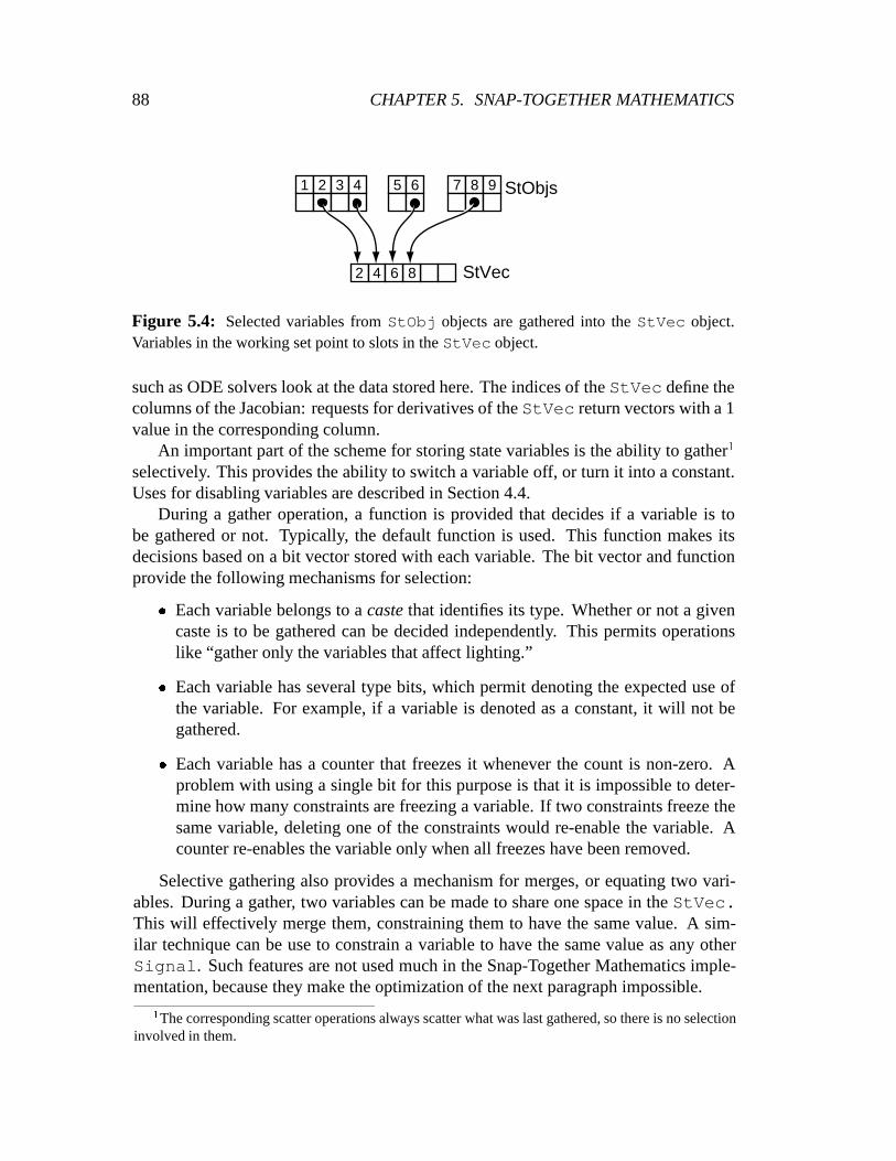
88 CHAPTER 5. SNAP-TOGETHER MATHEMATICS
1 2
2
3 4
4
7 8
8
95 6
6
StObjs
StVec
Figure 5.4: Selected variables fromStObj objects are gathered into theStVec object.Variables in the working set point to slots in theStVec object.
such as ODE solvers look at the data stored here. The indices of theStVec define thecolumns of the Jacobian: requests for derivatives of theStVec return vectors with a 1value in the corresponding column.
An important part of the scheme for storing state variables is the ability to gather1
selectively. This provides the ability to switch a variableoff, or turn it into a constant.Uses for disabling variables are described in Section 4.4.
During a gather operation, a function is provided that decides if a variable is tobe gathered or not. Typically, the default function is used.This function makes itsdecisions based on a bit vector stored with each variable. The bit vector and functionprovide the following mechanisms for selection:
� Each variable belongs to acastethat identifies its type. Whether or not a givencaste is to be gathered can be decided independently. This permits operationslike “gather only the variables that affect lighting.”
� Each variable has several type bits, which permit denoting the expected use ofthe variable. For example, if a variable is denoted as a constant, it will not begathered.
� Each variable has a counter that freezes it whenever the count is non-zero. Aproblem with using a single bit for this purpose is that it is impossible to deter-mine how many constraints are freezing a variable. If two constraints freeze thesame variable, deleting one of the constraints would re-enable the variable. Acounter re-enables the variable only when all freezes have been removed.
Selective gathering also provides a mechanism for merges, or equating two vari-ables. During a gather, two variables can be made to share onespace in theStVec.This will effectively merge them, constraining them to havethe same value. A sim-ilar technique can be use to constrain a variable to have the same value as any otherSignal . Such features are not used much in the Snap-Together Mathematics imple-mentation, because they make the optimization of the next paragraph impossible.
1The corresponding scatter operations always scatter what was last gathered, so there is no selectioninvolved in them.
5.4. THE SNAP-TOGETHER MATH LIBRARY 89
An important special case of a function block is one that has each of its inputsconnected to the sameStObj. This is a very common case, used often for graphicalobjects where the function blocks each compute some attribute. Because all of theinputs are connected to variables, the Jacobian of the inputs of the block is the identitymatrix, possibly with some columns missing. By exploiting this, the matrix multiplyto compute the block’s Jacobian can be considerably faster.This leads to substantialspeedups in many applications, as these direct-connected blocks are very common,and very often constitute the majority of the “wide” input blocks, which are the mostexpensive to compute.
Partitioning, as introduced in Section 4.3.3, reorders theelements of theStVec sothat variables in a common partition are next to one another,facilitating solving eachsubset independently. Partitioning is done only when a gather operation is performed,not each time the linear system is solved. This is done because re-ordering the statevector would confuse the process of differential equation solving.
Because the partitioning algorithm does not actually look at the values ofJ , theydo not need to be computed when finding the initial matrix to partition. In fact, ratherthan using the real values of the matrix, it can be better to use binary values whichrepresent that the matrix element might be non-zero, ratherthan that it is non-zero forthe current value of the state vector. This is easily achieved by having eachPortprovide a method which works like thegrad(int) method, but does a logical orinstead of a linear combination of its input vectors. For objects that do not provide thisoptional method, the gradient may be used instead.
5.4.4 Caching in Snap-Together Math
As hinted at in Section 5.4.1, caching is an important tool for enhancing performance inSnap-Together Mathematics evaluations. Whenever a value orderivative is computedby a function block, or otherPort type that implements caching, it is stored insidethe block in case the result is used again. Each time a value orderivative is requested,the block first decides if its cached value is valid; if it is, it avoids re-computation andsimply returns the cached value.
The Snap-Together Mathematics toolkit employs a simple cache validation scheme.A single global timestamp is used. Whenever any of the inputs (state variables) arechanged, this timestamp is incremented. A block must recompute if its internal times-tamp is older than the global timestamp. This scheme is very simple but has the obviousproblem that it invalidates much more than needs to be. Changing a single value inval-idates all caches in the entire system.
In the context of the differential approach, invalidating all the caches simultane-ously is not as catastrophic as it might seem since the variables are all updated simul-taneously with each ODE solver call for evaluation of the differential optimization.Schemes that do substantially better require some combination of substantial amounts

90 CHAPTER 5. SNAP-TOGETHER MATHEMATICS
of graph traversal, explicitly representing links bidirectionally, doing numerical andsparse data structure comparisons, or exploiting knowledge about the particular prob-lem. For most applications, such complication is not warranted as, at best, it serves onlyto reduce the constants on the linear complexity portions ofthe differential approach.
5.4.5 The Differential Solver
The Snap-Together Mathematics toolkit encapsulates the abstractions of the differentialapproach in a set of classes that implement the techniques ofthe previous chapters. Anobject is used to represent the differential optimization problem, storing informationabout the controls and the variables they effect. This object is called a constraint engineor ConstEngine.
The ConstEngine class has fields that contain anStVec and a list ofStObjthat are to be gathered for computations. AConstEngine object also stores infor-mation to define the objective function for the differentialoptimization, such as a listof Signals that make upg:
The controls for the differential optimization problem arestored in aConstEngineby a list ofController objects.Controllers are objects that specify desiredderivatives for connectors, as discussed in the next chapter. The Snap-Together Math-ematics class for a controller specifies aSignal to control, a controller type, andseveral parameters.
Solving the differential optimization problem, e.g. usingthe techniques of Chapter3 and Chapter 4, is executed by a method of theConstEngine class. This is theonly part of the system in which constraint solving needs to be done. This methodis implemented in a manner that interfaces with the ODE solver implementations ofthe underlying mathematics toolkit. TheConstEngine class also interfaces withnon-linear iterative solvers.
Snap-Together Mathematics is built on top of an object-oriented mathematics toolkitthat I wrote. The toolkit includes an object-oriented framework for defining ODE prob-lems and solvers. The classIntegrand represents an ODE problem by defining asingle method that defines a function to compute_
q given q and t: An ODESolverobject stores an integrand and an initial condition and offers a method to step timeforward. TheConstEngine class is a subtype ofIntegrand .
When used as anIntegrand to solve a differential optimization problem, aConstEngine must first load theq vector provided by the ODE solver into itsStVec. Loading the state allows the solver to try different values for the state inthe process of taking an ODE step. TheConstEngine keeps all of the intermediateresults of the solving process, such as the Lagrange multipliers, as internal fields.

5.4. THE SNAP-TOGETHER MATH LIBRARY 91
5.4.6 The Whisper/Snap-Together Math Interface
While Snap-Together Mathematics is a C++ toolkit, an interface is provided to it asan extension to the Whisper interpreter described in Appendix A. The extension addsseveral new data types to Whisper, as well as many new primitive functions.WhSTMprovides a convenient way to access to the functionality of the Snap-Together Mathe-matics, and can be used on its own to develop simple applications completely in Whis-per. The Whisper/Snap-Together Mathematics interface, called WhSTM,shows howthe functionality of Snap-Together Mathematicscan be provided in a more convenientform, and will be used in later portions of the thesis.
WhSTMprovides primitive Whisper data types for most the Snap-Together Mathe-matics classesPort , FBlock , StObj , Signal , andConst . Other classes, gener-ated by primitives written in C++ are generally treated by the more generic class thatis appropriate. For example, a summation block, which is notanFBlock because itallows variable numbers of inputs, simply appears as aPort in Whisper. No facilityfor defining new subtypes of Snap-Together Mathematics classes is provided in Whis-per. WhSTMdefines 88 primitives, including creation functions for 30 different typesof function blocks.
WhSTMsupports automatic promotion of types as needed. Any function requiringa Port can take anything that is a subtype, includingFBlock andStObj types,even though Whisper has no subtyping mechanism. Real numbersare also promotedto Port where necessary; a constant valued port object is automatically created.
The constructor forSignal takes aPort and an index. It permits specifying theindex either as an integer or as a string name if the block being connected to suppliedthe optional names for its outputs. If the index is omitted, it is assumed to be 0. Thisallows aPort to be promoted to aSignal when needed.
Function block creation routines all optionally take initial values for the signal in-put. The convenience of this, coupled with the automatic promotions, is demonstratedin this simple example
(set b (plus-block (times-block (signal point-port 2) 5)(signal point-port ’y)))
that computes the sum of 5 times thez value of a 3 output port representing a Cartesiancoordinate and itsy value. The ease with which functions can be built in Whisper willbe used in the Bramble toolkit, described in Chapter 7. A moreextensive example ofusingWhSTMto build function graphs is described in Section A.2.
The Whisper interface does not provide constraint engines orODE solvers as basictypes. However,WhSTMdoes have default instances of these objects, so that commandslike

92 CHAPTER 5. SNAP-TOGETHER MATHEMATICS
(add-const (controller sig ’= 2.0))
implies the use of the “built-in” constraint engine, and
(rk4-step .1)
uses the built-in 4th order Runge-Kutta solver instance to step the default constraintengine forward a time step. Other packages further extending Whisper can alter thedefaults. This will be used extensively in Bramble.

Chapter 6
If you don’t know where you’re going, you will wind upsomewhere else.
— Yogi Berra
Controllers
The previous three chapters provided the machinery required to implement the dif-ferential approach. This machinery permits specifying desired derivatives for func-tion outputs. Appropriate changes to the state of the objects are computed from thesederivatives. In this chapter, we consider how to specify thederivatives in order to creategraphical interaction techniques.
With the differential approach, graphical objects are manipulated by specifying howparticular attributes of the objects should change. Graphical objects provide their at-tributes as output connectors. A connector serves as a control when its behavior isspecified. The specification of the derivative of a connectoris encapsulated into anobject called acontroller. These objects are plugged into any connector output just asdependency inputs are. A controller can look at the output itis connected to and theexternal world (e.g. input devices) in order to produce a desired derivative value for theconnector.
The capabilities of a controller are limited: they can specify only a rate of change.Objects move by having controllers attached to their connectors over a period of time,continuously specifying derivative values which are converted by the differential opti-mization to derivatives of the object parameters.
The basic building blocks of graphical interaction techniques are controllers andconnectors. For the purposes of interaction, the set of graphical objects appears as aset of connectors, any of which can serve as controls by having a controller attached tothem. The chapter begins by showing how basic methods such asdragging are createdby attaching controllers to connectors for periods of time.Subsequent sections explainhow the continuous model of time is coupled with events and describes the details ofthe controllers themselves. Some details of creating complex controllers that switchcontrols on and off are discussed in the chapter’s final section.
93

94 CHAPTER 6. CONTROLLERS
Line State Vectorx1 y1 x2 y2
left right center length angle
l θx y x y x y
dist.
d
Line State Vectorx1 y1 x2 y2
left right center length angle
l θx y x y x y
Ruler
Figure 6.1: A schematic “wiring diagram” of two line segments with an attachment constraintbetween their endpoints. For the purposes of defining manipulations, these objects appear as aset of connectors awaiting controllers to be plugged into them.
6.1 Example Interactions
To show how the machinery of the differential approach applies to manipulating graph-ical objects, we consider some concrete examples. For theseexamples, our model willconsist of 3 graphical objects: two line segments, and an attachment object that is con-nected to one endpoint of each line segment. A schematic of the data structures is givenin Figure 6.1.
6.1.1 Specifying Values
A basic operation is to specify a value for a connector, for example to specify a positionfor an endpoint of a line segment. This cannot be done directly with the differentialapproach: only rates of change can be specified. In order to achieve a desired value,we must specify the derivative over a period of time, and waitfor the object to achievethe desired value.
TheGoTowards controller makes a connector’s value move towards a target.Ateach instant, it computes a derivative that moves the value towards the desired goal,as will be discussed in more detail in Section 6.3. AGoTowards controller doesnot specify its attached connector’s value. However, by pushing its value in the rightdirection, over time the connector will reach its target unless something impedes itsprogress. In order to specify a target value, we place aGoTowards and wait for the

6.1. EXAMPLE INTERACTIONS 95
value to reach its target.If the GoTowards controller is left attached after the attached connector reaches
its target, the controller will continue to drive the value towards the target, holding itin place. This is how constraints are created. Because theGoTowards continuallypushes toward the goal, the constraint will be restored if itdrifts. TheGoTowardscontroller, therefore, include constraint stabilizationlike that proposed by Baumgarte[Bau72].
To create a constraint, a controller must be applied to some connector. The at-tachment object which simply provides the connector is not ageometric constraint byitself. However, a geometric connection constraint objectwould be a version of the at-tachment object that createdGoTowards 0 controllers on its connectors when it wasplaced, and removed these controllers when it was removed.
6.1.2 Dragging
To drag an object, we can permit the user to specify where a particular point on itshould be positioned. When the mouse button is pressed to graba point on an object, adifferential controller is attached to the output that computes the position of the point.This controller guides the point to follow the mouse. When thebutton is released, thecontroller is removed from the output connector of the dragged point. The addition ofan optimization objective term with the mouse position to provide manipulation of agraphical object is first presented in [KWT88].
The Follow controller provides derivative values that cause its attached con-troller to move towards tracking a moving target. It is similar to aGoTowards , withthe exception that rather than having a fixed target, it has a moving target. This be-havior could be created with aGoTowards controller that periodically has its targetvalue updated. However,Follow controllers can sometimes provide better trackingbehavior by using information about the motion of its target. In the case of trackingan input device, where derivative information is difficult to estimate for lack of a goodpredictive model, aFollow controller is typically implemented as aGoTowards .More details about theFollow controller are provided in Section 6.3.
For many reasons, it is unlikely that the point being draggedwill track the cursorexactly. When the cursor moves quickly, it might take the system a few steps for thedragged object catch up, and even then, if the cursor moves far during the step, the twowill separate. Also, the rates at which graphical objects can move is sometimes limitedby how well the ODE solver can solve for the motion; if the object moves too quickly,the ODE solver will be unable to accurately compute its motion. Faster steps and betteralgorithms can reduce the separation, however the mouse might still separate from theobject being dragged if the motion is restricted by a constraint.
When the cursor and dragged point diverge, it is important to provide visual feed-back to connect them. Typically, a line is drawn between the cursor and the point being

96 CHAPTER 6. CONTROLLERS
Figure 6.2: A small line is used to connect the mouse pointer to the objectbeing dragged.This feedback is important because the cursor location willdiverge from the location of theobject because of lag, integration error, or restrictions on the object’s motion.
dragged, as shown in Figure 6.2. Metaphorically the cursor is connected to the draggedpoint with a rubber band. This metaphor is a pretty accurate one for the spring attractiontechniques introduced in Section 3.5.1.
The generality of the differential approach is apparent in the simple example ofdragging. Graphical objects provide point position aspects. The dragging behavior canbe plugged into any objects’ output. The differential solving process will compute howto control the objects’ parameters in order to achieve the desired motion. If a differentpointing device, for example a 3D tracker, is available, it too could be plugged in to thesame places.
6.1.3 Constrained Dragging
The ability to mix constraints and controls is important to the effective use of con-straints. The constraints permit the user to drag objects without violating any previ-ously established relationships. User defined persistent constraints can provide manyservices, including helping to avoid redundant work, helping to explore a constrainedspace, or helping to construct compound objects.
Because constraints are easy to attach and detach, they can be used with drag-ging controls to define interaction techniques. In additionto creating aFollow orGoTowards controller to cause the mouse to be tracked, additional constraints aresimultaneously added. These constraints are removed when the dragging controller isremoved.
For an example, consider rotating a graphical object. To create a rotation, the objectcould be dragged subject to a constraint that nails the position of its center in place.Dragging points on the object will then cause the object to rotate, assuming the objecthas that degree of freedom. Dragging might also cause the object to stretch, if thedragging motion is not circular about the center of rotation. This can be combatted bykeeping the cursor on a circular track or by using another constraint to keep the sizeconstant. In the latter case, some mechanism that makes the dragging constraint breakrather than the others will be required. The dragging control must be subject to theother constraints. Techniques for achieving this are discussed in Section 3.5.
The ability to combine constraints and controls allows a setof building blocks to be

6.2. CONTINUOUS TIME 97
Mouse Down Event
Mouse Up Event
Follow Controllers Created
Follow Controllers Removed
Object Moves
Figure 6.3: A timeline of an interaction in the differential approach. The arrow symbolizesthe flow of time. At discrete instants, such as when the mouse events are received, the setof differential controllers is altered. The effects of these over time causes changes in objectconfigurations.
provided for constructing interaction techniques. For example, it provides a constraint-based strategy for developing 3D manipulation techniques,as discussed in Chapter8. The basic idea is that enough constraints are provided so that the input device issufficient to fully determine the motion. This strategy is not unlike what we employ inthe real world where we use things such as jigs and braces to help us manipulate hardto handle objects.
6.2 Continuous Time
As illustrated by the above examples, object configurationsare altered by having con-trollers specify their behaviors over a period of time. The state of objects cannot bechanged instantaneously. Instead, it changes over time, the way an object in the realworld does. This is quite different than traditional methods for constructing interac-tive systems, where the state of objects is updated at discrete instants corresponding toevents or polling increments.
In concept, time in the differential approach continuouslymoves forward. Whiletime progresses, any active differential controllers are causing the objects they affectto change. At discrete instants, such as a window system event, controllers may becreated, destroyed or altered, however, the state of objects is not changed. To changethe configuration of an object, a controller must be created and time must pass so thatthe object can adjust itself accordingly. A time line of sucha process is depicted inFigure 6.3.
Since a controller can be plugged into any connector at any time, placing a controllercan be asynchronous with the placement of other controllers. This makes it easy to

98 CHAPTER 6. CONTROLLERS
Mouse Down Event
Mouse Up Event
Follow Controllers Created
Follow Controllers Removed
Object Moves
Figure 6.4: A timeline of interaction in the differential approach, as actually implemented.The arrow symbolizes the flow of time. Time is discretized into steps. A discrete event isdeferred until the end of the step it occurs in.
perform concurrent operations, such as allowing for asynchronous two-handed input.In practice, we can only approximate the continuous flow of time discretely. As
discussed in Section 3.3, we must treat the ordinary differential equations describingobject trajectories as a sequence of steps in order to solve them. During each step, timeis advanced a small amount. By making these steps small enough, the user is given theillusion of continuous motion.
As implemented in the differential approach, events are deferred until the end of thestep, as depicted in the timeline of Figure 6.4. If the duration of the steps is very small,the delays will not have an effect. If avoiding this lag is crucial, the approach can bemodified slightly to trade total number of steps for reduced lag. For example, whenan event occurs, the current step could be aborted and later restarted after the eventis processed. Also, time may be stopped during periods when no objects are movingand user events are expected. For example, in a standard direct manipulation system,when the user is not dragging an object, nothing is moving so differential time may bestopped and the system may spend its full effort responding to events. An event mayneed to start time, for example if it initiates a dragging operation.
After each step, the system must redraw the displays. For theprototypes of thisthesis, screen update always redraws the entire display. Other systems might attemptto speed redraw by selectively updating only objects that have changed. I have nottaken such an approach because:
1. Selective redisplay is more difficult with the differential approach since many ob-jects may be moving at once. In fact, the system must be able todetermine whenselective redraw is appropriate, and when it would simply befaster to redraw theentire view.
2. Selective redraw is difficult to implement for 3D applications when using a Z-

6.2. CONTINUOUS TIME 99
buffer hidden surface removal algorithm, because the stateof the Z-buffer mustbe restored when objects are removed from the display.
3. The differential approach has been based on the assumption that fast drawinghardware is available.
6.2.1 Differential Time and Clock Time
The time in the differential approach is advanced at each ODEsolver step. There is noassurance that the “clock” in the differential approach, that is the time that passes fromsolver steps, will correspond to wall-clock real time. In fact, making differential andreal time correspond would be difficult: a system would have to be able to accuratelypredict how long (in real time) it will take to do the computations required for each step,and make sure the proper amount of differential time advances on each step. This rulesout the possibility of the system adaptively controlling time steps when things growdifficult, and would require complicated synchronization when the real world clockand the differential time differ.
Rather than coupling differential time and real time, we instead let the clocks float.The differential “clock” can be thought of as a dimensionless quantity: it’s mapping to“wall clock” time is unknown, and unimportant. Whether the clock moves quickly andvelocities are low, or the clock moves slowly and velocitiesare high, the same effectscan be achieved. It becomes impossible to express controls in terms of real time, forexample to say that an object moves across the screen at 3 inches per second, or thata point reaches its target in 250 milliseconds. However, other imprecisions also makethis impossible, both spatially (how far is 3 inches when theuser can scale the windowor run on a different monitor) and temporally (how can we be sure that in that 250milliseconds the system will not have to swap or process a higher priority job). Whilemulti-media systems researchers, such as [DNN+93], are beginning to study with suchreal-time issues, the differential approach, like most interactive graphics systems, is notconcerned with real-time performance. Coupling with real time is left for future workin Section 10.3, but a simple approach would take a step as fast as possible and thenwait for the real time clock to catch up.
6.2.2 Breakdown of Interactivity
The differential approach relies on being able to provide a large number of steps persecond. This is needed both to provide the illusion of continuous motion to the user, andto insure events are processed without too much lag since they are deferred to the end ofa step. As the introduction to this thesis states, modern computers continue to provideincreasing amounts of graphical and numerical processing capabilities. However, eventhough the capabilities of computers may continue to grow exponentially, the types of

100 CHAPTER 6. CONTROLLERS
problems that users are interested in tackling may similarly grow without bound. Asthe task grows, the amount of computation required to support differential interactionalso grows. At some point, processing each step requires toomuch time and the qualityof interaction suffers. This is calledinteractive breakdown.
It is difficult to determine precisely the rate at which interactive breakdown oc-curs. Even when the motion appears jerky, it can sometimes beacceptable, dependingon the user and the problem. For some applications, high frame rate is crucial, forexample when the motion is needed to help the user comprehendthe behavior of ob-jects. Similarly, event delay lag is most bothersome when the user is generating manyevents in rapid succession or that are time critical, such asselecting a moving object.As described in Section 6.2, event processing lag can be reduced at the expense ofthroughput.
As the complexity of the problem goes up, so does the time required to do each step.The immense scale of the objects that people design – a modernjet airplane may havemillionsof components[Hei93] – makes keeping interactive rates impractical for someproblems. However, the limitations of the human cognitive and perceptual abilitiesmake it unlikely that a user would want to operate a model of that scale interactively.The prototype implementations show that models of reasonable complexity can be han-dled on the current generation of computers. Performance ofthe prototypes is discussedin Appendix B.
6.3 Basic Controllers
Controllers are objects which attach to connectors and specify values for their deriva-tives. The examples of Section 6.1 briefly introduced some types of controllers. Here,we examine these controllers in more detail, introduce a more complete set of con-trollers, and discuss how they compute the derivative values.
Since a controller’s sole function is to provide a derivative value, deciding whatvalues to specify is the critical issue in designing a controller. This is complicated bythe fact that interface elements are traditionally not defined by derivatives, but rather bypositions. Another issue in picking velocities is that simulation time is not coupled toreal time in a meaningful way, as discussed in Section 6.2.1.This makes it impossibleto specify velocities in terms of apparent velocities, although this would be attractiveto insure that the user can follow the motion. However, the more relevant speed limitis typically given by the ODE solver, as discussed in Section3.3.
The simplest controller provides a constant derivative value. TheseConstantcontrollers are rarely used because attributes typically do not move at fixed veloci-ties regardless of other factors, and determining specific velocity constants is difficultbecause time and space do not precisely correspond to real-world quantities. In thecases where they are used,Constant controllers are typically given values which

6.3. BASIC CONTROLLERS 101
are found empirically to produce a desired rate in certain situations. The more com-mon controllers do not inherently specify a time, but rathera target and provide thecontroller with flexibility in choosing the velocity that achieves it.
More useful controllers examine the value of the connector they are attached toin order to select a derivative value. The two basic varieties of such controllers areGoTowards andFollow . Each of these picks derivative values to make its attachedconnector achieve a target value. The difference is that aGoTowards has a fixedtarget, whileFollow has a moving target such as a motion path or an input device.An important distinction is that aFollow may be able to use information about themotion of its target in order to track better.
A GoTowards controller picks its control velocity to get its value to thedesiredtarget. The value of the velocity must be related to the distance of the control fromthe target. There are several ways to choose the value. One isto pick a velocity thatgets the control to its target in a set amount of time. The amount of time must be longenough to encompass a sufficient number of solver steps, and not too fast such thatODE solver inaccuracies cause the control to overshoot its target.
An alternate method of choosing the velocity for anGoTowards controller is tomake it a scaled factor of the displacement. This creates spring-like attraction. Whenthe control is far away it moves quickly, facilitating coarse positioning. As it gets close,it moves more slowly for precise positioning. One drawback of this technique is thatit is hard to achieve target exactly: when the control is veryclose, its velocity is verylow. One solution used in the prototypes is to switch betweenspring attraction andthe constant rate scheme described above. When a control getssufficiently close to itstarget, its velocity is chosen so that it would achieve the goal exactly in a step. Thisworks well because for these small displacements, the approximations that the ODEsolver makes may be sufficiently accurate.
An important attribute ofGoTowards controllers is that they implicitly incorpo-rate feedback. That is, they are continually adjusting the velocities to correct for anyerrors. If numerical drift or some other problem causes a control to make a turn for theworse, the error will be corrected in subsequent steps. Because of this, constraints willalmost always use aGoTowards controller rather than aConstant controller withconstant derivative 0.
An approximation to aFollow controller can be created with aGoTowardscontroller whose target is periodically updated. However,Follow controllers notonly build in this continual update, but provide an opportunity to incorporate knowledgeof the target’s trajectory to improve tracking. AFollow controller effectively drivesits value towards where its target will be, rather than whereit is. In order to do this, thetime derivative information of the target must be known. In practice, we rarely havegood enough predictive models of input devices for this to work; however, it is usefulfor tracking key-framed motion paths, as described by [WW90].
102 CHAPTER 6. CONTROLLERS
6.4 Switching Controllers
The controllers we have discussed so far continuously perform the same simple taskwhile plugged in. In this section we consider some more complex controllers thatswitch themselves on and off based on the values of the connector they are attachedto and some measures of how hard they are working. In effect, these complex con-trollers simply plug and unplug more basicGoTowards controllers as needed. Thesebehaviors are encapsulated as new controller types because: they are widely useful, soa simple encapsulation is handy; they can continuously watch the values, potentiallyswitching more often than just at step boundaries; and they will look at internal solverquantities, the Lagrange multipliers, that we might prefernot to expose to system com-ponents outside of the solver.
By being clever about when controls are switched on and off based on the valueof the connector they are attached to, a variety of interesting behaviors can be cre-ated. One behavior that this allows creating is an inequality constraint or boundary ona value. Switching of equality constraints is a standard technique for implementinginequality constraints, and is referred to as theactive setmethod by the numerical anal-ysis literature as it keeps a subset of all the constraints active at any given time. For thedifferential approach, we use similar techniques to createother behaviors as well. Thissection begins by describing three different variations ofactive set techniques, and thendiscuss some of the challenges in implementing them correctly.
6.4.1 Bounding
Placing boundaries or inequalities on aspect values is often useful, for example when arange of values is illegal, or only an approximate range is known. ABound controlleris created by enabling aGoTowards controller whenever the value has moved pastthe boundary. TheGoTowards controller is used to move the value back within theboundary. When the output is within the legal region, the boundary constraint doesnothing. The other major complication is that the boundary constraint should neverpull the value further into the violated region, as depictedin Figure 6.5. That is, ifanother controller is trying to pull the value out of the illegal region, the boundarycontroller should not fight it. This case must be handled within the differential solver,as discussed in Section 6.4.4.
Inequality constraints operate by first being violated and using aGoTowards tofix themselves. If a value is moving towards a boundary, theGoTowards does notenable until after it has violated the boundary. One solution to this problem is that ifsuch a violation is detected, back time up until the value is exactly at the boundary. Thisprocedure is often done for physical simulation of collisions, as discussed in [Bar92b].Such backing up could be used with the differential approach, and is discussed morefully in Section 6.4.5.

6.4. SWITCHING CONTROLLERS 103
Figure 6.5: The point is bound to remain inside the rectangle. Left: whenthe point is inan illegal position aGoTowards controller pulls it back to the boundary of the legal region.Right: if some other controller will pull the point back intothe legal region, aGoTowards
controller that attempts to pull the point to the boundary ofthe legal region would pull againstthe other controller, and is therefore disabled.
6.4.2 Snapping
One of the fundamental issues in direct manipulation is precision: how can exact val-ues be specified when they are required. This problem arises in many situations, forexample when attempting to establish a precise geometric relationship in a drawing,when picking a small object, or when attempting to hold an object steadily in placewith a noisy input device. One solution that has been employed to provide precision indirect manipulation is known gravity fields or snapping.
Gravity fields were first introduced in Sketchpad[Sut63]. Interesting points have agravity field that draws the cursor in when it is close. The cursor follows the pointingdevice, however, when it is close to an interesting locationit “snaps” precisely there.Many varieties of snapping have been used to help in direct manipulation. The mostcommon are grids, which snap the cursor to points on a grid. Another important varietyis object gravity, in which the cursor is drawn towards the graphical objects.
Just as we rely on tools such as straight-edges, rulers, and compasses to aid a pencilin drawing a precise drawing, gravity or snapping serves as atool for creating precisegraphical manipulations. Rather than having to manipulateobjects to exact positions,the user can simply get them close, and the gravity takes the job of precisely position-ing the cursor. This allows drawings to be created with more precision than the inputdevice has, or to have precision even if the input device is noisy. Interface issues insnapping, such as providing feedback so the user can be confident that the correct re-lationship is being established and selecting among many close-together snap targets,can be handled, as shown in theBriar drawing program of Section 9.1.
One obvious way to incorporate snapping with differential manipulation is to usethe snap target as the goal for dragging. This approach was used in theBriar drawingprogram, described in Section 9.1. One complication is thatsince the dragged object

104 CHAPTER 6. CONTROLLERS
does not follow the cursor exactly, the object may not establish the relationship that thecursor does. This can be combatted with feedback to inform the user when the draggedpoint establishes the relationship that the cursor has, andby making the snapping persistlong enough to allow the dragged point to catch up with the cursor.
It is also possible to use the differential approach to implement snapping. A con-troller is connected to drive the output to a precise value when the output gets close. Ifanother controller attempts to pull the connected attribute from its target, the snappingcontroller is disabled. An analogy for this is pushing a marble around on a groovedtable. When the marble is close to a groove it falls into the groove, and will roll aroundinside of it until pushed hard enough that it escapes from theslot.
A Snap controller is implemented using a variant of the active set technique usedfor Bound controllers. By default, the controller is inactive. If thevalue of its at-tached connector gets within a specified distance of the snapping target, the controlleris activated and switches on aGoTowards controller to drive the connector to thetarget value. If the magnitude of the Lagrange multiplier for the GoTowards everexceeds a limit value, the controller is pulling too hard against other controllers andmust be deactivated.
The key intuition behindSnap controllers is that the Lagrange multiplier is a mea-sure of how hard a control is pulling. Since the “pull” of a controller is actually deter-mined by the product of the Lagrange multiplier and the gradient of the control function,the magnitude of this vector is actually used to determine the amount of effort the con-troller is applying. One difficulty withSnap controllers is that the parameters thatdetermine their behavior, most specifically the limit magnitude, must be determinedempirically.
A Snap controller can be attached to any object output, not just positions. Forinstance, aSnap controller on a line segment’s orientation could make a segment thatwas easy to place into a precisely horizontal configuration.The differential implemen-tation provides more flexibility than traditional methods for implementing snapping.We therefore call the differential snappinggeneralized snapping.In Section 8.4.1 wediscuss some applications of generalized snapping.
6.4.3 Click Stops
Another way to combat the precision problem with direct manipulation is to require avalue to have one of a discrete set of values, for example to create a grid for dragging.This is easy to do with the traditional implementations of direct manipulation, whichoften use integer representations anyway. However, the differential approach operateson continuous values. One way to implement an interaction that limits a value to adiscrete set isclicking.
Clicking is a variant of snapping that effectively constrains a connector output tohave a discrete value, either from a finite set, or to be an integer or multiple.Click

6.4. SWITCHING CONTROLLERS 105
1 2
λ
1 2
λ
1 2
λ
(a) (b) (c)
Figure 6.6: Clicking forces a value to be in a discrete set. The value, in this case the horizontalposition of the circle, is constrained to have the value 1 or 2. Grey arrows represent the pullof the mouse control, black arrows represent the pull of theClick controller. Initially (a) ithas value 1, so aGoTowards controller pulls to maintain this value as the mouse attemptsto drag it with a pull labeled�: At some point, the mouse pulls hard enough so that the pullvector’s magnitude exceeds a limit value causing the controller to advance to the next clickstop (b), causing the point to attain the next value in the set(c).
controllers work by constraining the output to have a value in the set. If the constraintis pulling too hard, the value is changed to another element in the set, as illustrated inFigure 6.6.
6.4.4 Implementing Active Set Methods
The Bound , Snap, and Click controllers all operate by switching simplerGoTowards controllers on and off. They are all variants of the active set methodscommonly used for realizing inequality constraints. Active set algorithms are detailedin standard textbooks such as [GMW81] and [Fle87]. The difficult part of such algo-rithms is determining which constraints to enable and disable, a combinatorial problem.The simple method discussed here tries a few guesses at the correct set, and then givesup, selecting a solution that fails to satisfy all the requirements. The solver will be likelyto provide an acceptable interactive behavior. We will, therefore, begin by examiningthe active set problem in the context of the differential approach, and then describeda simple algorithm. While the simple technique does guarantee the correct answers tothe problems, it has the following advantages:
� The methods always fail in ways that can be corrected later.
� The methods are easy to implement as extensions to the existing differential op-timization.
� The methods do not access any of the matrices, except by calling the differentialoptimization. Therefore, as with the differential optimization techniques, we canuse any linear system solver.

106 CHAPTER 6. CONTROLLERS
(a)
qa=0
(b)
qa=0
(c)
qa=0
Figure 6.7: An inequality constraintqa
> 0 keeps the block above the floor. The inequalityis implemented by switching an equality constraintq
a
= 0 on and off. When the block isabove the floor (a), the equality constraint is inactive. If the block is on or under the floor (b),the constraint pushes the block towards being on the floor, counteracting any controls that arepulling the block downwards. However, if other controls attempts to pull the block above thefloor (c), the control used for the inequality would pull downward, causing sticking. Therefore,it is deactivated.
Recently, an inequality solver specifically designed for interactive systems was de-veloped by David Baraff [Bar94]. The algorithm was designedfor implementing phys-ical simulations of collisions, a problem very similar to implementing graphical manip-ulation with the differential approach. Baraff’s algorithm could be used in computingthe differential optimization. Application of this algorithm to implementing the dif-ferential approach is left as a topic for future study (Section 10.3). However, withoutsignificant work, such algorithms do not have many of the advantages of the iterativesolvers discussed in Section 4.3.2, such as the ability to exploit sparsity.
Active Set Methods in the Differential Approach
To introduce the basic idea of an active set method, considerthe simple example ofFigure 6.7. The example has a single state variable,q
a
that measures the block’s heightabove the floor. An inequality constraint is used to keep the block above the floor,q
a
> 0: An active set method implements this inequality by switching the equalityconstraintq
a
= 0; or in differential termsqa
GoTowards 0; on and off as needed.If the block is above the floor, the inequality constraint does nothing. It isinactive.
The more interesting case is when the block either sits on thefloor, or has fallen belowthe floor. In this case, theGoTowards controller is activated to either push the blocktowards sitting exactly on the floor, or to prevent the block from sinking underneath

6.4. SWITCHING CONTROLLERS 107
the floor. When the constraint works to keep the block above thefloor, its Lagrangemultiplier will be positive, that is, the constraint is pushing upwards.
Consider a case where the block is sitting on the floor, with the constraint activated.Suppose another control, such as connection to the mouse, attempts to pull the block offthe floor. TheGoTowards controller will attempt to keep the block on the floor, witha negative Lagrange multiplier pulling downwards. In essence, the inequality constraintwill be sticky. The solution to this is to disallow negative Lagrange multipliers. Whenone is found, the constraint must be deactivated.
When there are multiple inequality constraints coupling objects, deciding whichLagrange multipliers to deactivate becomes more complicated. Consider the exampleof Figure 6.8. Two keep the two blocks stacked, one inequality constraint keeps block Babove the ground, while the other keeps block A above block B.The former constraintis implemented by switching the equalityq
b
= 0 on and off, the latter by switchingq
b
� q
a
= h: For each solution of the Lagrange multipliers, the solver must determinewhich of the two constraints should be activated. If a control is used to pull blockA upwards and both constraints are active, the equality constraints would maintainthe stacked configuration, causing the blocks to stick in place by pulling downwardon them. Since the inqualities can only push upwards, we might deactivate the onespulling downwards (e.g. both of them). However, deactivating all of the constraintspulling in illegal directions is unnecessary, and wrong. Ifthere is a soft control pullingB downwards, that constraint should stay active.
The process of determining the active set is iterative: the solver must determinewhich ways the constraints are pulling, deactivate any constraints pulling in illegaldirections, reactivate any constraints that should not have been disabled, and repeat.Determining the correct active set can be difficult, and might require many attempts.
If the correct active set is not found, there are two types of errors possible for anyparticular constraint. Either a constraint that should be active is deactivated, or a con-straint that should be inactive is activated. This latter case is extremely problematic.Consider what would happen in the example of Figure 6.7: the user would not be ableto lift the block off the floor. If the algorithm made this error in one step, it would makethe same error in subsequent steps since the configuration does not change1.
Deactivating too many constraints is less of a concern. Consider the example ofFigure 6.8. If both constraints are deactivated, the lower block will not be preventedfrom moving downward for the step. However, in the next step,the algorithm couldcorrect for this error. It is unlikely to make an error activating the constraint becausethe block will be separated from the upper block, which is what caused the confusion.
If we resign ourselves to not always being able to find the correct active set, wemust at least make sure to always err on the side of deactivating too many constraints.Such an algorithm is simple to devise. An example algorithm is presented in the next
1Assuming the algorithm is deterministic and it bases decisions solely on the configuration, whichthe differential methods do.

108 CHAPTER 6. CONTROLLERS
qb=0
(a)
qa-qb=hqa-qb=h
qb=0
(b)
qa-qb=h
qb=0
(c)
qa-qb=h
qb=0
(d)
Figure 6.8: Multiple blocks are kept stacked on the floor by inequality constraints. (a) Oneconstraint keeps block B above the floor, the other keeps block A above block B. (b) If acontrol pulls upwards on block A, the active constraints impose equalities that cause the blocksto stick in place. (c) Removing all inequalities that are pulling downward in (b) would causethe constraint on block B to be erroneously removed. If another control were pulling down onit, no constraint would keep B above the table. (d) The correct solution reenables constraint B.
section.It is important to notice that excess deactivations are onlya problem when there
are many interacting inequality constraints. There are interesting applications, suchas collision simulation, where this occurs. In such applications, these errors might beproblematic. However, there are other potentially more significant sources of errorsin such applications, such as improperly handling the piecewise continuous nature ofthe ODEs, as discussed later in this section. In Section 8.4.2, we will look at using thedifferential approach for collisions, and consider the problems.
An Active Set Algorithm
The basic outline of a simple active set technique is as follows:
1. Select an initial active set by activated any inequality constraints that may be ac-tive. Candidate constraints are those whose values either violate their boundariesor are within a tolerance of the boundaries.
2. Select some deactivated constraints that are potentially active and reactivate them.
3. Solve for the Lagrange multipliers.

6.4. SWITCHING CONTROLLERS 109
4. Deactivate any constraints with negative Lagrange multipliers.
5. If the active set was changed, return to step 2.
The simplest method omits step 2. This leads to a method that meets the requirementthat it will always err on the side of having too few active constraints. It also is guar-anteed to terminate because on each iteration the size of theactive set must decrease,since there is no step inside the iteration that adds constraints. It has the disadvantagethat it often removes too many constraints.
A constraint is a candidate for reactivation in step 2 if the derivative of the functionis negative. A constraintf
i
(q) > k is a candidate for reactivation ifrf
i
�_q < 0:
Implementing reactivation can be complicated. The method must not to cycle, thatis to infinitely loop among several active sets. A method thatI have used to preventlooping is to permit a given constraint to be reactivated at most once. While this fallsfar short of a reliable inequality solver, it gets correct solutions on many problems onwhich the simpler method fails, for example the problem of Figure 6.8.
6.4.5 Piecewise Continuous ODE Solving
Solving the ODE is difficult because the derivatives are continually changing. In Sec-tion 3.3, we were concerned about them changing due to the functions being non-linear.However, the derivatives might also change discontinuously when the set of controlschange. Such ODEs are calledpiecewise continuousas they consist of continuouspieces between breaks. Note that the discontinuities are inthe derivatives, not in thevalues. Methods for solving piecewise continuous ODEs are discussed in an appendixof [Bar92c].
An ODE solving technique such as Runge-Kutta attempts to fit acontinuous func-tion (a polynomial) to the ODE over a step. If the ODE is discontinuous, this may beproblematic. Even if multiple smaller steps are taken to fit the function with piecewisepolynomial segments, methods that take fixed step sizes are not likely to have theirdiscontinuities match the discontinuities in the derivatives.
Many of the discontinuities are avoided in the differentialapproach, since eventsthat change the set of controls are deferred until the ends ofsteps. The ODEs aretherefore step-piecewise continuous, or continuous within the steps. This means thattechniques such as Runge-Kutta are acceptable, because they will not see the disconti-nuities. Techniques that require continuity between steps, such as Predictor Correctormethods, may have more problems.
Active set methods may change the set of controls during a step, causing a dis-continuity in the derivatives. This is potentially problematic. However, the alternativewould involve finding the precise time that the controls switch and adapting the stepsizes so that the step boundaries occur exactly at this instant.

110 CHAPTER 6. CONTROLLERS
The most severe symptom of not finding discontinuities is that the system can re-spond to changes only after they happen. For example, an inequality constraint acti-vates after it is violated. Therefore, there will be a brief instant when the constraint isviolated. Subsequent steps will move to a it valid state. Theill-effects of an ODE solvermisfitting a continuous polynomial will similarly be repaired by subsequent steps. Ifsuch error is unacceptable, cleanup steps can be used.
Piecewise ODE solving by backing up can be used with the differential approach.I have instead used the approach of letting later steps correct for any errors caused byviolations. There are many reasons to prefer such an approach:
� The general root finding problem of determining when to back up to is difficult.
� The ill-effects of adaptive step sizes, as described in Section 3.3.1 are applicable- possibly even more so as adjusting the step size requires a potentially timeconsuming root finding operation.
� When there are many changes close together in time, a backing-up system cantake only tiny steps between them. In a cleanup afterwards approach, many canbe cleaned up simultaneously.
� With the cleanup approach, objects not affected by the discontinuity continue tomove as they otherwise would. If the step size were adapted, all of the objectswould slow down whenever any discontinuities occurred.
For certain applications, such as collision simulation, having instants of violated in-equalities will be unacceptable, and piecewise ODE methodswill be required.
Chapter 7
But the ancient debate on emergence, whether indeedwholes may have properties not intrinsic to the parts, isbesides the point. The fact is, that parts have propertiesthat are characteristic of them only as they are parts ofwholes; the properties come into existence in the interac-tion that makes the whole.
— Richard Levins and Richard LewontinThe Dialectical Biologist,p 273
A Graphics Toolkit
To this point, we have introduced the machinery of the differential approach, the meth-ods for its realization, and the structure of a general purpose implementation. In thischapter, we consider how the approach can be encapsulated tosupport the constructionof graphical editing applications. Graphical applications typically share a wide varietyof functionality, so their construction is often facilitated by the creation of toolkits thatencapsulate the common needs. This chapter discusses such atoolkit built on top ofthe differential approach.Brambleis an object-oriented graphics toolkit, built on theinfrastructure of the previous chapters.
Bramble has much in common with other object-oriented graphics toolkits designedto support direct manipulation graphical editors, such as Garnet [MGD+90], Inventor[SC92], GROOP [KW93], and Alice [PT94]. Bramble’s primary distinction is that itis designed on top of the differential approach. The major consequences of this are:
� The differential approach is used to create almost all graphical manipulations.
� Graphical objects have connectors that compute their various attributes, and oftenprovide these standardized connectors in lieu of specific interaction code.
� Snap-Together Mathematics is used to connect objects together and to connectinteractive controls to objects.
� Bramble provides support for application features such as geometric constraintsthat are easy to create with the differential approach, but difficult to implementin standard toolkits.
� Bramble’s control flow is dictated by the differential approach. The model of anODE solver with events interleaved between steps, as described in Section 6.2,
111

112 CHAPTER 7. A GRAPHICS TOOLKIT
provides a centralized main loop that calls application code when needed. Thedifferential approach allows continuous motion direct manipulation to fit nicelyinto such a scheme. callback style architecture as mechanisms exist that permitdirect manipulation to fit in such a scheme.
Bramble not only shows how the machinery of the differentialapproach can beapplied to the construction of graphical applications, butalso how the approach’s ma-chinery can be encapsulated and hidden from the applications programmer. My goalsin constructing Bramble were:
� To make it possible to quickly prototype a number of applications to illustrateand explore the differential approach. The emphasis is on speed of constructionand extensibility, rather than on industrial strength tools. Much of this goal waspragmatic: I needed to construct enough examples to supportthe conjectures ofthis thesis in a reasonable amount of time.
� To support a variety of applications. It was important that Bramble could sup-port both 2D and 3D applications. While the focus is on graphical editors andmodelers, Bramble also supports other applications such asobject viewers andvisualization tools.
� To support the basic services of graphical applications typically provided bytoolkits.
� To facilitate building applications that provide the features that the differentialapproach supports, such as geometric constraints.
� To facilitate experimenting with interaction techniques and evaluating them incontext within applications.
� To show how the architectural features of the differential approach could impactapplications architecture. In particular, the approach can enable increased mod-ularity, since Snap-Together Math provides a common connection mechanismbetween parts, and separation of manipulation and representation aids encapsu-lation.
� To show that the machinery of the approach can be sufficientlyencapsulated. Theapplication programmer does not need to see the mathematicsin order to makeuse of the approach’s features. Bramble is designed to let developers programwith the familiar abstractions of graphical applications.They see the abstrac-tions of the approach only when defining new interaction techniques. Brambleprogrammers never need see the inner workings of the solver.

7.1. THE BRAMBLE APPLICATION MODEL 113
7.1 The Bramble Application Model
The flow of control in Bramble is dictated by the differentialapproach, as describedin Section 6.2. Time flows forward as the ODE solver steps forward, continuouslyevolving the state of the objects. By continuously viewing the world as it evolves, wecan see objects move according to their controls. At discrete instants, such as when anevent occurs, changes to the objects in the world can be made.However, such eventsare instantaneous impulses: all changes to the configurations of objects must happenvia the passage of time by the ODE solver.
The differential approach’s model of time is significant in toolkit design for tworelated reasons:
1. It provides a uniform “main loop” for all applications.
2. It provides a way to incorporate simultaneous, continuous actions such as drag-ging into an event driven architecture. Events can asynchronously begin andend continuous motion actions, concurrency is handled by the solver: there is noneed for multi-threading or other time sharing mechanisms to achieve concurrent,asynchronous actions.
These two elements make it practical for Bramble to use eventcallbacks as its soleapplication control mechanism. A Bramble application doesnot contain a “main” loop,but rather, after the application concludes its initial setup, it simply call a functiondefining a standard loop that runs the ODE solver, keeps the views of the world upto date, and calls appropriate fragments of application code when needed. Code to becalled is specified in hooks, variables that can be bound to fragments of code that areaccessed at defined times. Hooks are discussed in more detailin Section 7.6.
The overall structure of Bramble is shown in the schematic ofFigure 7.1. Brambleis built on top of the Silicon Graphics GL graphics library [Sil91] and the Snap-TogetherMath toolkit, discussed in Chapter 5. Bramble itself contains no solver code and doesnot even provide access to the solver’s internal structures. Bramble also includes theWhisper embedded interpreter, described in Appendix A. The symbiosis of Brambleand Whisper will be discussed in Section 7.1.1.
A Bramble application consists of two parts:
� Code implementing any custom classes.
� A program that is run to execute the application. This program typically sets upthe application, doing tasks like opening windows, creating initial objects andwidgets, and defining hooks. After initialization, the program starts the differen-tial process’ time flowing. Once time is started, application code is only executedwhen a hook is called.

114 CHAPTER 7. A GRAPHICS TOOLKIT
Snap Together Math (includes differential solver)
Whisper interpreter toolkit
Application Application Application Application Application
Bramble
Standard Objects Application Specific Objects
Object Management
Application Support windows widgets standard interaction techniques
GL
Figure 7.1: The pieces of the Bramble toolkit. Bramble is built on top of Snap-TogetherMath and the Whisper interpreter. It contains a variety of pre-defined object classes, supportfor managing sets of graphical objects, and other miscellaneous pieces needed by graphicalapplications. A Bramble application typically consists ofa Whisper driver program and (op-tionally) C++ definitions of new object types.
The major pieces of Bramble are akin to other similar toolkits. Each is affected bythe use of the differential approach:
Object Management – Bramble’s mechanisms for managing sets of objects, discussedin Section 7.3, provide access to the features relevant to the differential approach,such as keeping track of state variables and connectors. Allobjects, even win-dows and widgets, can have state and connectors.
Standard Object Types – Bramble’s standard object types, discussed in Section 7.5provide a wide range of connectors to support graphical manipulation.
Hooks – Bramble provides a set of hooks that aim to be sufficient to specify a range ofinteraction techniques. These are chosen to provide a convenient set of opportu-nities to alter the controllers and objects of the differential approach. Bramble’shooks are discussed in Section 7.6.
Windows and Widgets – Bramble’s windows can contain views of the world that areautomatically kept consistent, and many of the supported widgets, such as sliders,are designed to manipulate their targets using the differential approach. Thesefeatures are described in Section 7.7.

7.1. THE BRAMBLE APPLICATION MODEL 115
Standard Interaction Techniques – Bramble contains many basic graphical manip-ulation techniques in its library, all of which are defined with the differentialapproach. Picking and snapping services are tuned towards the selection of con-nectors for manipulation.
This chapter will discuss these various pieces of Bramble, following a discussion of animportant part of Bramble’s structure, and a simple exampleof how Bramble is used.
7.1.1 Whisper and Bramble
The Whisper embedded interpreter, described in Appendix A, is an important part ofBramble. An embedded interpreter is a useful feature for graphical applications as itprovides support for features such as saving and loading user data files and user exten-sions. However, Whisper plays an even more significant role inBramble. Internally,the Whisper interpreter’s implementation is used by Bramblefor support, and exter-nally, much of the application programming in Bramble is done in Whisper.
As discussed in Section 2.3, using an embedded interpreter in a graphics toolkit isa common technique. However, the differential approach removes some of the draw-backs. The speed-critical computations occur as part of themathematics; all standardpieces can be written in the compiled host language. The centralized main loop pro-vided by the ODE solver also interacts nicely with the embedded interpreter. Mostapplication behavior is defined by hooks. Bramble’s hook mechanism, discussed inSection 7.6, permits pointers to C++ functions, text fragments of Whisper code, andWhisper closures to be dynamically assigned.
Like other similar languages, Whisper has a runtime support system for memoryand object management. Bramble also uses these facilities for its needs. The advan-tages are twofold: first, it provides Bramble with a dynamic,memory managed objectsystem; and second, it means that Bramble’s objects are easily accessible from the in-terpreter.
The majority of Bramble application programming is done in Whisper. Brambleis designed such that applications are constructed by extending the generic default ap-plication. Constructing applications in the extension language is, therefore, sensible.Application programming in Whisper has many advantages:
� The interpretive nature of Whisper leads to faster turnaround than the staticallycompiled C++ environment.1
� The interactive loop of the interpreter provides a useful debugging environment,whereas the complexity of the entire C++ system makes using the standard C++debuggers awkward.
1This is more a statement about the C++ programming environment at the present time than aboutBramble.

116 CHAPTER 7. A GRAPHICS TOOLKIT
� Whisper’s abstraction mechanisms, notably first-class functions and dynamic ob-jects, are useful in the design of interactive systems.
� Many of the details of the system are hidden from a Whisper programmer. Forexample, window management and refresh, and the solver internals are hidden.In fact, there are no mechanisms provided in Whisper to accessinternal solverdata structures. The language does not even have vector or matrix constructs!
There is nothing thatmustbe done in Whisper. However, almost all application pro-grammingcanbe done in whisper.
Bramble is actually wired into the Whisper interpreter as an extension. The C++“main” of a Bramble application is a Whisper read–eval–printloop, typically that canselect files to read from the command line. For my work, there is a single Whis-per/Bramble executable and each application differs only by the Whisper program usedto run the application. For many applications, however, a different version of the inter-preter, with custom sets of extensions wired in, would be more desirable.
The interpreter-based organization of Bramble emphasizesthat it meets its goals ofinsulating the application from the mathematics. The differential optimization is com-pletely encapsulated inside theConstEngine object as described in Section 5.4.5.Nowhere in the Bramble toolkit source code or applications is there mention of theinternals of the solver process.
7.2 A Simple Example
In order to introduce the basic concepts of Bramble, a simpleexample will be presented.This example is designed to be similar to that used to introduce the Inventor toolkit. Inthe Inventor book [Wer94], a program called “hello cone” is given as a first introductionto Inventor. Here is the same program, one that displays a cone in a window, writtenwith Bramble:
(1) (set my-view (make-view ”Hello Cone”))(2) (set my-cam (make-la-camera))(3) (view-cam my-view my-cam)
(4) (set c (make-cone))(5) (c (set material shiny-red-material))
(6) (go)
This simple example brings out the basic notions of Bramble.A program placesgraphical objects in the world, and does not worry about lower level details such as howthey are drawn or how the windows are managed. The first line creates a window that

7.2. A SIMPLE EXAMPLE 117
Figure 7.2: The simple “Hello Cone” program in Bramble.
views Bramble’s world. Line 2 creates a default “lookat” camera, and line 3 specifiesthat the view created on line 1 should look at the world through the lens of this camera.
Lines 4 and 5 of the program create the cone object, and changes its color to red.The color is changed by setting the property of the cone object that specifies the surfaceproperties to be a predefined material that is shiny red. Thisunusual syntax for access-ing object fields is described in Appendix A. Notice that whenthe cone is created, it isby default created in the world and is therefore visible to viewers of the world.
The “action” of the program takes place in the last line. Thego routine beginsthe interactive loop which is in the toolkit proper. In differential terms, time is started.Steps are continually taken, and in between any events are handled. The interactiveloop runs continuously until either the program is killed, or a flag is set.
The simple 3D example receives a lot of a 3D interface from Bramble’s defaults, asshown in Figure 7.2. By default, Bramble creates a number of interface elements suchas the ground plane, some lights, and the shadows dropped vertically onto the groundas if the sun were at high noon. These defaults can easily be overridden. In a sense, theBramble program simply modifies the default application andruns it.
The most obvious difference between this program and the Inventor equivalent isthat it is written in Whisper, not C++. This difference can be emphasized by adding theline
(add-key dev-esckey k-any k-down(lambda (v) (set bramble-going nil)))
which attaches a procedure that sets a flag to the escape key. This flag signals thegoroutine to stop the interactive loop and return. Since thereis no code after the callto go , Bramble will return to an interactive Whisper prompt. This allows a user tointeractively alter the program. The differential interactive loop can be restarted withanother call to thego routine.

118 CHAPTER 7. A GRAPHICS TOOLKIT
To get elements of a standard 3D interface, some standard keydefinitions can beread by replacing lines 1 through 3 with
(read std-world.wh)(set v (make-standard-view ”Hello Cone”))
at the top of the file. The Bramble standard 3D interface, described in Section 7.8binds the mouse buttons to routines that permit objects to begrabbed and dragged andthe viewpoint to be controlled.
With the 3D interface, we would notice that when we grab the cone in the simpleprogram, it does not move. The primitive cone from the library is a rigid body thathas no degrees of freedom. To make it movable, we place the cone in a transformationgroup with the lines
(set g (make-qs-group))(add-to-group g c)
somewhere after the cone is created, but beforego. Themake-qs-group functioncreates an empty group that can rotate and scale (qs stands for quaternion and scale).
We might want to have the cone begin pointing upwards. Since this will require anon-differential change (i.e. we want it to instantaneously appear in the right orienta-tion), we cannot use the differential machinery. This meanswe must actually directlyaccess and modify the state variable of the object. This is done by
(set-qvar (get-q g) ’sy -1)
that sets thesy (scale in y) variable of the group to -1. We might then want to preventthe object from scaling as it is manipulated, which can be accomplished by
(freeze-scale g)
which is a special operation for groups.The cone can now be grabbed and dragged using the standard Bramble mousepole
manipulation technique, as described in Section 7.8. We will now add some otherfunctionality that uses Bramble to operate the differential machinery. Suppose that wewant to have the top of the cone fly towards the left. This is accomplished by taking aconnector that computes the position of the top of the cone and attaching a controllerto it. Since the cone object has a predefined “top” connector,this operation is as easyas
(controller (signal (c top) ’x) ’= 5)
that finds the x coordinate output of the top connector of the cone and creates a con-

7.2. A SIMPLE EXAMPLE 119
troller that drives it towards the value 5. We might want to instead bind this operationto a key so it happens only when we’re ready
(add-key dev-gkey k-none k-down(lambda (v) (controller (signal (c top) ’x) ’= 5))).
Notice how this example maps exactly to the abstractions of the differential approach.We manipulate an object by attaching controllers to its connectors. The actual changeitself happens as time passes after the discrete instant when the controller is created.The manipulation is done completely in terms of the connectors of the objects, withoutregard for what parameters inside make them actually change.
Suppose we want to make a chain of cones. Here, we add a second cone and connectit to the first.
(set c2 (make-cone))(set g2 (make-q-group))(add-to-group g2 c2)(pt-eq (c bottom) (c2 top))
The important thing to notice from this example is that we were able to create theconnection by talking in terms of geometric or graphical objects, not mathematics. Theconstraint is created to connect the bottom of one cone and the top of the other.
The lack of mathematics in the last example is a result of us being fortunate that thecones had the connectors we desired. However, adding a new connector is easy enough.Suppose we wanted to add a new “horizontal” connector to the cone that measured ifthe cone was horizontal (i.e. that the y coordinate of its topand bottom are equal, asBramble’s coordinate systems defines the y axis to mean height). This can be done as
(c (bind horiz (minus-block (signal top ’y)(signal bottom ’y))))
This code fragment uses the Whisper/Snap-Together Mathematics interface to create aSnap-Together Mathematics output that computes a new attribute calledhoriz . Theattribute is computed by subtracting the height of the bottom of the cone from the top.A function block is used to perform the subtraction. Whisper scoping rules cause thecode fragment that creates the block to be executed in the cone’s environment, so thattop andbottom refer to the cone. The code fragment stores stores the function blockas a field in the cone object’s environment permitting other objects to access it to useit as a connector. This code fragment could be written as a procedure that could beapplied to other cones

120 CHAPTER 7. A GRAPHICS TOOLKIT
(define add-horiz (a-cone)(a-cone (bind horiz (minus-block (signal top ’y)
(signal bottom ’y)))))
These connectors could be used just as any others, for example
(add-horiz c2)(controller (c2 horiz) ’= 0)
7.3 Bramble’s World
The focus of Bramble is on building object-oriented graphical applications. One ofBramble’s central roles is to help maintain the set of objects that are being presentedto the user. In Bramble, there is a single, implicit “world” in which all objects exist.By default, when objects are created they are placed in the world. The concept ofthe world is implicit in Bramble, unlike Inventor which requires explicit creation of“scene graphs.” The advantage of this is simplicity, although the ability to have multiplesimultaneous worlds is sacrificed.
The world provides a uniform 3D coordinate system for all objects. The world isalways 3D, even for 2D applications. In such applications, objects ignore the thirddimension. This has a small cost, for example in doing transformations. The benefitsinclude avoiding redundant code and the ability to place 2D objects in 3D worlds. Theunderlying GL graphics toolkit takes a similar approach.
In Bramble, the programming model is not of screens that are continuously redrawn.Instead, the model is of a time continuous world into which objects are placed andmanipulated. Images on the screen provide views of this world.
7.3.1 The Bramble Object System
The mechanisms that support state variables, connectors, and other object managementare implemented at a general level. This permits all major object types in Bramble,including windows and widgets, to support features that areusually associated withgraphical objects, such as having state and connectors.
All major types of objects in Bramble are subclasses of the typeIDObj . Having acommon base allows common functionality to be shared among all types of objects. Forexample, each object has the ability to be named, and is assigned a unique ID numberthat serves as a soft pointer (hence the nameIDObj ). EachIDObj has a field thatallows its major subtype to be determined dynamically. An object manager keeps trackof all IDObj s created. The major subclasses ofIDObj are:

7.3. BRAMBLE’S WORLD 121
Drawable – a graphical object in world space. This includes not only theuser createdscene objects, but lights, cameras, hierarchy elements, and world space interfaceelements such as 3D widgets.
IDrawable – a special object that exists in screen space, rather than in world space.Effectively, these objects are attached to lenses of cameras.
View – an object representing a view of the world on the screen. It isbasically apairing of a camera and a window, with added responsibilities for determiningdrawing parameters.
DistinguishedPoint – an important type of connector that represents a specificpoint on some object.
Imagepoint – a special type of connector that represents the position on the screenof a point.
SubWin – a subwindow of a screen window. Subclasses include widgets like buttonsand sliders.
Frame – the “physical” GL window on the screen. May contain severalSubWins,one of which may be aView.
Material – a set of surface properties.
Demon– a special object that performs its hooks when triggering events occur.
One of the key ideas behind Bramble’s object management is that each IDObj con-tains a Whisper environment. In Whisper, environments serve as a dynamic objectsystem (see Appendix A). Using Whisper environments as an object system for C++has several advantages:
� It provides easy access to the object from Whisper.
� By defining methods as values in the Whisper object, they can bedynamicallyaltered.
� Fields and methods can be added and removed dynamically as needed.
� Objects can inquire about which fields and methods other objects contain.
� Whisper environments, to a certain extent, are automatically memory-managed.
The dynamic nature of objects is important: fields and methods may be added in re-sponse to user actions. It also allows experimentation withapplication behavior: ob-jects can be interactively modified while the application isrunning.

122 CHAPTER 7. A GRAPHICS TOOLKIT
Any IDObj can have state variables and connectors. The base class handles man-agement of these differential features. It also permits objects to create differential con-trollers or employ function blocks. These are automatically removed when the objectis deleted. Object deletion is also handled by the base classusing lists of hooks. Thispermits an object to define work that must be done when the object is removed. Dy-namic definition of deleters, very much in contrast to the static C++ notion of a deletermethod, is a very useful feature.
Memory management can be a difficult task in an interactive system. Brambleuses a variety of manual techniques to automatically managememory without usinga garbage collector. Bramble contains mechanisms to deal with the inverse garbagecollection problem. An inverse garbage collector activates when an object must bedeleted, for example in response to a user command, and insures other objects thatrefer to it are appropriately altered or deleted. A garbage collector does not provide thisbehavior. In fact, in a system that was simply garbage collected, the object would not bedeleted until all references to it were removed. Interconnection of objects is pervasivein and central to the differential approach, so handling inverse garbage collection isimportant in Bramble. The mechanism used to handle this problem is to have eachobject maintain lists of other objects that should be notified or deleted when the objectis deleted.
7.3.2 Graphical Objects
The graphical objects in Bramble’s world are derived from the classDrawable . Thisclass requires only a few methods. Subclasses ofDrawable define a draw methodthat needs only to operate in the object’s local coordinate frame. Objects may also pro-vide other functionality. For example, most objects will define at least a few connectorsso they can be manipulated, and will allocate a state vector to store their configuration.Other examples of optionalDrawable functionality include ray intersection, bound-ing box computation and generation of external representations. Almost all methodsapply in local coordinates. Hierarchy mechanisms perform required conversions auto-matically.
Bramble keeps all of the instances ofDrawable on a list. The list of “the stuff”is Bramble’s notion of a scene. Only one list is kept by the program. Selective draw-ing can effectively provide multiple scenes. Although the list is a flat representation,hierarchies are supported by the grouping mechanism, described in Section 7.5.3.
The graphical objects are not unlike their counterparts in other object-oriented graph-ics toolkits. One difference in Bramble is that each object class does not have to providemethods for interaction. An object need only provide connectors that the more generalmanipulation techniques can connect to. “Object-centric”styles of interaction are pos-sible with Bramble. For example, an application can have each object define methodswhich are called by a dispatcher that receives events. Intermediate styles, for example

7.4. CONNECTORS IN BRAMBLE 123
having an object use hooks to alter general manipulation techniques, are also possible.Another distinction of Bramble’s graphical objects is thatthey must also manage
state and connectors in ways that permit the differential approach to manipulate theobject. Bramble’s object system provides a uniform place for objects to keep a statevector. Once a graphical object registers that it has a statevector, Bramble automati-cally insures that the variables are managed correctly.
Connectors are handled in a less uniform manner. In Bramble,a connector is simplya Snap-Together MathematicsPort that an object stores in a way that other objectscan gain access to it. Standard mechanisms exist for certainimportant types of connec-tors, as discussed in Section 7.4.
7.4 Connectors in Bramble
In Bramble, a connector is simply a Snap-Together MathematicsPort that an objectexposes in a way that other interested objects can gain access to it. The most commonway to do this is for the object to place thePort in a field of its kept environment.Objects are free to create any types of connectors they want.Objects often providespecial purpose connectors tuned to compute their specific types of attributes. Manyspecific examples are given in Section 8.1.
The most important type of connector in Bramble is thedistinguished point.ADistinguishedPoint represents a particular point on a graphical object. Theprimary output of aDistinguishedPoint object is its position in space, but in-stances usually provide other attributes, such as surface normals and tangents, whenthey are known.
Distinguished points are first class Bramble objects unto themselves, that also hap-pen to bePort objects as well. By being a realIDObj a distinguished point can:
� be accessed by standard object naming and reference techniques;
� store state, permitting the point to be moved around on the object;
� define hooks to specify its behavior;
� have other connectors associated with it, for example, to compute the position ofits shadow on the floor or wall.
To standardize access, each object keeps a list of its distinguished points. Similarly, aglobal list of all distinguished points is kept to aid in suchtasks as picking and snapping.Registry in this global list is automatically handled by theDistinguishedPointcreation process, and permits points to be found by name or bylocation.
The position and orientation of a distinguished point are not simply a function ofthe graphical object the point is on, but also the transformations applied to the object.

124 CHAPTER 7. A GRAPHICS TOOLKIT
However, the hierarchy mechanisms automatically handle these transformations. Apoint must provide only methods for computing its connectors in the object’s localcoordinate frame. Jacobians are also composed for points inhierarchies.
Standard subclasses ofDistinguishedPoint include:
Fixed Points that are a fixed position in the object’s local coordinate system.
Point on Point that connect directly to a set of object variables that represent a posi-tion.
Free Points that store their position in the object’s local coordinate space as their ownstate vector. Constraints are often used to keep such pointsin the volume of oron the surface of an object.
Different types of objects may also define special types ofDistinguishedPoint .For example, a parametric surface might define a type of pointthat stores its parametervalues as state. Such a point can slide along the surface, or the parameters can be frozento create a fixed point.
7.5 Graphical Objects
Bramble supports a wide range of graphical objects. Many standard subtypes ofDrawable are provided, and new application-specific types can be defined.
7.5.1 Standard Object Types
Bramble predefines a variety of basic object types, along with standard connectors withwhich to manipulate them. For example, the 2D set includes lines, circles, rectangles,ellipses, and polygons. A general parametric curve class allows the definition of newobject types by simply providing the parametric function. Connectors and a drawingfunction are defined automatically from this as described inSection 8.1.1.
Most of the standard 3D objects are defined as rigid bodies that must be placedinside of groups to be moved. Most standard shapes, such as cones, tori, cylinders, andspheres are provided. Polyhedra can be defined in several ways, including readers forseveral data file formats.
A planar mirror is provided as a 3D rigid object. In terms of its geometry, the mirroris simply a rigid square. However, the mirror’s draw function calls other objects’ drawfunction with a new transformation that draws the object on the mirror’s surface tosimulate reflection. Mirrors define special connectors thatpermit the reflections to bedirectly manipulated.
Geometric constraints are represented byDrawable objects which create asso-ciated controllers on some of their connectors. For example, a connection constraint

7.5. GRAPHICAL OBJECTS 125
would take twoDistinguishedPoint position connectors, and compute the dif-ference as a connector. When created, it would also create aGoTowards controlleron the distance connector to maintain the constraint. The objects that represent con-straints may provide drawing methods that provide feedbackto the user. Bramble in-cludes many basic constraint objects in two and three dimensions, including point con-nection, distance, collinearity, normal or tangent alignment, and parallel. Inequalityconstraints in the basic set include constraints to keep points inside many of the basicshapes. All of these constraints operate generically on object connectors so they canbe attached to many types of objects.
7.5.2 Defining New Object Types
Many applications will need special purpose object types not included in the standardset. For example, the planar mechanisms simulator of Section 9.2 defines special ob-jects for mechanical parts such as motors, linkage rods, andsliders. Often these objectsare simply slight variations on the standard toolkit objects. For example, a linkage rodis simply a line segment that is drawn in a different way and has its length constrainedto be fixed at creation.
Most of the standard functionality ofDrawable objects can be implemented inWhisper, allowing new types of objects to be dynamically defined. For example, thefollowing code defines a new type ofDrawable that is a simple 2D line segment.
(1) (defun make-line (x1 y1 x2 y2)(2) (let* ((obj (wh-drawable 'line))(3) (q (make-stobj 4)))(4) (set-qvar q 0 x1 y1 x2 y2) (5) (caste-vars q vc-sceneobj)(6) (brobj-add-vars obj q)
; procedure to create a line ; create an empty object; make a 4 place state vector; put initial values into state; declare type of variables; install variables in object
(16) obj))
(12) (bind-in (get-env obj) drawf(13) (lambda (draw-flags)(14) (prog (move (val q 0) (val q 1)) (15) (draw (val q 2) (val q 3)))))
(9) (bind-in (get-env obj) length(10) (dist2d-block (signal q 0) (signal q 1) (11) (signal q 2) (signal q 3)))
(7) (point-on-vars-2d obj 0 1)(8) (point-on-vars-2d obj 2 3)
; define draw method; function of draw params; use GL move/draw commands; to draw line
; define a length connector; compute with distance block
; return created object
; create point connectors; one for each endpoint
This defines a procedure that creates an instance of the new type, given initial po-sitions for its endpoints. It first creates an “empty” object(line 2) and a state vector

126 CHAPTER 7. A GRAPHICS TOOLKIT
(line 3) that contains space for 4 variables. The object represents the line by the po-sitions of the endpoints, so the initial values can be placeddirectly into the variables(line 4). Lines 5 and 6 declare the type of the variables and install them into the object.Lines 7 and 8 createDistinguishedPoint connectors for the endpoints. Theseconnectors can obtain their values directly from variablesin the state vector. Lines 9through 11 create a length connector by computing the distance between the two end-points. Lines 12 through 15 define a draw method for the line segment. The methodtakes a single argument, the drawing mode, that it ignores since it uses the defaults.
To facilitate the creation of new 2D objects types, Bramble provides a specialdefine-shape function, detailed in Section A.2.1. It provides a concise syntax forspecifying how the shape is drawn and placing connectors on it. The syntax permitsintermediate variables to be specified for convenience and internal constraints on theobject to be defined.
7.5.3 Groups
Bramble supports object hierarchies with itsGroup class. AGroup is a subclassof Drawable which contains a list of other objects and a transformation to apply tothem. Like the hardware and graphics library it has been built on, Bramble presentlysupports only linear transformations. EachGroup has a connector that computes itstransformation matrix from its state variables. DifferentGroup types define differentfunctions, for example to employ a quaternion or an Euler angle representations forrotation.
TheGroup class automates the process of building graphical hierarchies.Groupobjects manage the hierarchy for their member objects. For example, the membersneed only draw in their local coordinates as the group ensures that the proper trans-formations are applied before the object draws itself, permitting the graphics hard-ware to handle the transformation hierarchy. Making sure that the correct results occurwhen position or surface orientation connectors are computed is more complicated.TheDistinguishedPoint class handles this automatically.
Bramble’s grouping mechanisms make it simple to build hierarchies. Adding anobject to a group requires simply
(add-to-group group obj)
and everything is configured correctly. Similarly the ungrouping operation
(remove-from-group group obj)
does all of the required hierarchy management. One complication with ungroupingis that when the transformation is removed, the child objectmight jump in space. Toprevent this, each object keeps a matrix that contains any previously applied transfor-

7.5. GRAPHICAL OBJECTS 127
mation. This matrix is calledleftStuff since it represents what was to “the left” ofthe object when it was drawn.2 When an object is removed from a group, the group’stransformation is premultiplied into the object’sleftStuff matrix. This way theobject does not jump when ungrouped. TheleftStuff matrix is inserted into thematrix stack as each object is drawn.
Each different type ofGroup needs only to define its function that computes itsmatrix from its state variables. Some auxiliary information, denoting which variables,if any, correspond to rotation, translation, scaling, or center may also be provided.Bramble’s standard set ofGroup types include rigid body transformations (translateand rotate) with both quaternions and Euler angles, rotate/translate/scale transforma-tions, and a slider transformation that restricts objects to translate along a vertical linefrom the normal of a given point.
7.5.4 Cameras and Lights
A camera in Bramble is not just a 3D element. It is used for all transformations be-tween the world coordinate system and screen coordinates. Like aGroup , a BrambleCamera’s primary distinction is a function that maps from its state variables to atransformation matrix. In the case of aCamera, however, this transformation is fromworld space to screen space. The inverse of this matrix is used to draw the camera, forexample when another camera is looking at it.
The computer graphics literature is filled with many camera models. However,Bramble does not need to support a huge variety because the differential approachmakes them unnecessary. As best exemplified by Blinn’s work on spacecraft fly-bys[Bli88b], alternate formulations of a camera model are usedto provide parameterswhich serve as convenient controls for the user. With the differential approach, a singlecamera model can be used with a variety of interactive controls. By mixing and match-ing controls, the user can specify camera positions as conveniently as with special pur-pose formulations. The through-the-lens camera controls of Section 8.1.4 provide abuilding block from which many camera manipulations can be created, including thoseof Blinn’s paper as well as the more common LOOKFROM/LOOKAT model.
Bramble provides a small number of standard camera transforms. Orthographictransformations are provided to produce 2D images, as well as front, top, or side viewsof 3D scenes. The most common models in computer graphics define camera positionby a rotation about the eye point. Models differ in how they represent the rigid bodyconfiguration of the camera. Bramble provides camera representations based on quater-nions and Euler Angles. Usually, the quaternion representation is used because of itsattractive mathematical properties, but an Euler angle representation is also available,mainly for expository purposes.
2I use the postmultiply or function application notation, where the point to be transformed is writtento the right of the list of matrices.

128 CHAPTER 7. A GRAPHICS TOOLKIT
A common representation of the orientation of a camera in computer graphics is tostore a “look at” point that is to appear in the center of the image. A camera parameter-ized by LOOKFROM/LOOKAT is provided by Bramble. However, the functionalityis typically obtained by employing a Quaternion camera and athrough-the-lens con-trol, because the representation has better mathematical properties. The primary useof theLookAtCam is when the configuration of the camera is going to be staticallyconfigured in a program, rather than manipulated. In such a case, the programmer willtype the numbers that configure the camera, and therefore will require an easy to typerepresentation.
Like cameras, lights are represented by graphical objects within the scene. ALightobject is a special type ofDrawable that has an extra method which initializes thegraphics hardware to use the light. Lights provide information for optional shadowgeneration as a special connector which denotes the “bulb position” in homogeneouscoordinates to allow for distant light sources.
Bramble supports several types of light sources, corresponding with the capabilitiesof the GL graphics library and some of the renderers used. TheBramble light classesare: point lights, distant lights, directional spot lights, and ambient light. As graphicalobjects in the scene, point and spot light sources can be manipulated and transformedas other graphical objects. This allows placing lights in “fixtures,” like the Luxo lampof Section 1.1. Special connectors for manipulating lightswill be described in Section8.1.5.
7.6 Hooks
Bramble’s interaction model most closely resembles a dispatcher or notifier model[FvDFH90] where an application registers callback procedures with a centralized dis-patcher that calls the appropriate procedures at the appropriate times. Bramble uses thismodel for most application behavior, permitting an application to specify functionalityand then delegate the flow of control to the main ODE solver loop.
The callback mechanism in Bramble is through Whisperhooks. Like their LISPnamesakes, Whisper hooks are variables that can be given procedural values that arecalled at appropriate times. In Bramble, the hook mechanismallows either a pointer toa C++ function or a whisper closure. Often a variable stores alist of hooks to be called,rather than just a single hook.
By defining behavior with hooks, rather than hard-coded routines, the behavior ofan application can be dynamically altered. A goal in the design of Bramble was toprovide a sufficient set of hooks such that all post-setup application behavior can bedefined with hooks. This is more practical with the differential approach because timecontinuous activities are taken care of by the passage of time, so manipulation actionsare discrete events that can be tied to hooks. Only in extremely rare cases do hook
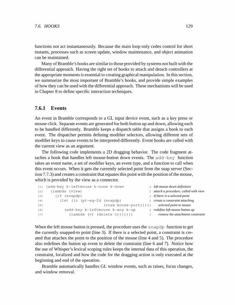
7.6. HOOKS 129
functions not act instantaneously. Because the main loop only cedes control for shortinstants, processes such as screen update, window maintenance, and object animationcan be maintained.
Many of Bramble’s hooks are similar to those provided by systems not built with thedifferential approach. Having the right set of hooks to attach and detach controllers atthe appropriate moments is essential to creating graphicalmanipulation. In this section,we summarize the most important of Bramble’s hooks, and provide simple examplesof how they can be used with the differential approach. Thesemechanisms will be usedin Chapter 8 to define specific interaction techniques.
7.6.1 Events
An event in Bramble corresponds to a GL input device event, such as a key press ormouse click. Separate events are generated for both button up and down, allowing eachto be handled differently. Bramble keeps a dispatch table that assigns a hook to eachevent. The dispatcher permits defining modifier selectors, allowing different sets ofmodifier keys to cause events to be interpreted differently.Event hooks are called withthe current view as an argument.
The following code implements a 2D dragging behavior. The code fragment at-taches a hook that handles left mouse-button down events. The add-key functiontakes an event name, a set of modifier keys, an event type, and afunction to call whenthis event occurs. When it gets the currently selected point from the snap server (Sec-tion 7.7.3) and creates a constraint that equates this pointwith the position of the mouse,which is provided by the view as a connector.(1) (add-key k-leftmouse k-none k-down(2) (lambda (view)(3) (if (snapdp)(4) (let ((c (pt-eq-2d (snapdp) (5) (view mouse-port))))(6) (add-key k-leftmouse k-any k-up(7) (lambda (v) (delete c)))))))
; left-mouse down definition; attach a procedure, called with view; if there is a selected point; create a constraint attaching; selected point to mouse; redefine left-mouse button up; remove the attachment constraint
When the left mouse button is pressed, the procedure uses thesnapdp function to getthe currently snapped-to point (line 3). If there is a selected point, a constraint is cre-ated that attaches the point to the position of the mouse (line 4 and 5). The procedurealso redefines the button up event to delete the constraint (line 6 and 7). Notice howthe use of Whisper’s lexical scoping rules keeps the internaldata of this operation, theconstraint, localized and how the code for the dragging action is only executed at thebeginning and end of the operation.
Bramble automatically handles GL window events, such as raises, focus changes,and window removal.

130 CHAPTER 7. A GRAPHICS TOOLKIT
7.6.2 Object Hooks
Event hooks are defined on a per-application basis. By default, an event handler doesnot provide different behavior based on the object being referenced. However, it isoften useful to provide behavior on a per-object basis. Sometoolkits, such as Inventor[SC92], dispatch events directly to objects to facilitate the diversity of object behavior.
To support diversity of object behavior, Bramble permits objects to specify hooksthat are called when certain operations are performed on them. Most of these, such asthe save hook, the draw hook, or the deleter hook are primarily useful for dynamicallycreating a new class of graphical object, as shown in Section7.5.2. Certain applicationspermit objects to define specific event hooks and perform the dispatching themselves.For example, the Showoff application, described in Section9.7, permits each objectto define a method to be called when the right mouse button is clicked on it. Theapplication defines the right mouse event handler to determine which object should benotified of the event, and to call the appropriate hook.
One set of standard event handling hooks that is particularly useful for defininginteractive behaviors with the differential approach is the grab/ungrab pair. Unlike theexample code of the previous section, the standard built-indrag handlers permit objectsand specific points to specify hooks that are called before a dragging operation is begunand after it has ended. This is often used to apply constraints that should act during thedragging. Some examples of how this is used are provided in Section 8.3.6.
Object hooks can be defined on a per instance basis, permitting individual instancesto each have their own behavior. Because hooks can be defined dynamically, the be-havior of an object can be altered while the program runs.
7.6.3 Demons
A Demon is a special class of object that causes hooks to be called when certain condi-tions occur. The common condition for aDemon is that a signal is within a thresholdof a desired value. EachDemon can define three main hooks:
do which is called when the condition the demon is looking for occurs. The demonremoves itself after calling this hook.
fails which is called if the demon is removed before its condition is satisfied.
done which is called when the demon is removed.
Demons have an optional timeout which causes them to be removed after a specifiednumber of steps, whether or not their conditions have been achieved.
Demons are useful for creating a variety of behaviors. One use of aDemon isto create a non-persistent constraint by removing aGoTowards controller after itachieves its goal. For example, to make example of Section 7.2 non-persistent so that

7.7. OTHER APPLICATION COMPONENTS 131
the cone can be freely manipulated after its top reaches the left edge of the table, wecould
(set cl (controller (signal (c top) ’x) ’= 5))((demon) (bind done (lambda (x) (delete cl)))
(bind tolerance .2)(bind lifetime 50)(bind possessed cl))
In this example, after creating the controller, a demon is created that “possesses” it.When the controller gets within tolerance of its target, or when the demon’s specifiedlifetime of 50 steps times out, the demon’s done hook is called, deleting the controller.Demons are also often used to remove constraints that are unable to be satisfied, per-mitting the application to give up.
7.6.4 Other Hooks
Much of the behavior of an application is defined by hooks. Most of these hooks areused for tasks not particular to the differential approach.For example, eachViewdefines a hook that draws the background of the image when its screen is cleared. Anyof these hookscouldcontain code that alters the set of controllers. However, a smallset seems useful for defining interaction techniques. The set includes:
sub-step-hook is called before each call to the differential solver (e.g. each substep ofthe ODE solver). This hook could be used to create active set methods, althoughhooks do not have access to solver internals to access the Lagrange multipliers.
step-hook is called after each step. One common use of the step-hook is for peri-odically altering aGoTowards controller to achieve the effect of aFollowcontroller.
add-obj-hook is called each time a new graphical object is added to the system. Thiscan be used to permit automatic registering of new connectors.
redraw-hook is called each time a view is redrawn. This is called once per view perstep as all views are updated each step in Bramble. This is often used to providefeedback to the user by drawing an overlay.
7.7 Other Application Components
Most of Bramble is concerned with providing support for the graphical objects whichthe user will actually place into models. However, there areother supporting objects,such as windows and buttons, which applications require andBramble supports. Many

132 CHAPTER 7. A GRAPHICS TOOLKIT
other toolkits provide similar support for these things; relevant aspects of how they arehandled in Bramble will be mentioned briefly. The emphasis inthe development ofthese objects is in providing tools which will allow these parts of applications to bebuilt quickly, so that more effort can be concentrated on thedevelopment of graphicalmanipulation techniques with the differential approach.
7.7.1 Windows, Views, and Widgets
Bramble contains an object type called aFrame which represents a window systemwindow object. A frame can contain many subwindows. One of these subwindowsmay be aView where Bramble draws a depiction of the current state of the graphicalobjects. EachView has an associated camera and attributes which determine howthe image is rendered. There can be many views at once, but each must have its owncamera and frame.
Frames andViews are first class objects in Bramble. In fact,Views always haveconnectors that provide the position of the mouse relative to the coordinate frame ofthe window. This simplifies attaching other connectors to the mouse.
A Frame can contain other subwindows besides aView . These are used to pro-vide buttons and other widgets around the edges of theView . All behavior of thewidgets is defined by hooks, including the widget’s appearance. These subwindowhooks include methods for drawing, handling mouse clicks, and a “tick” function thatis called periodically. Like the graphical objects, the predefined subwindow widgetsare designed to automatically update themselves to maintain a consistent view of thevalues that they access. The provided set includes:
Buttons that watch the value of a Whisper variable, and update automatically.
Radio Buttons that watch a variable and allow its value to be selected from aset.
Differential Sliders that can attach to connectors and create controllers in response tomouse clicks. These sliders permit not only dragging a connector’s value, butalso nailing or bounding it, as discussed in Section 8.2.1.
Color Sliders that create a set of differential sliders for RGB values along with feed-back for what the color is.
Text Elements that allow static display of information.
A special type of widget is provided to help watch the status of an object’s statevector. TheVarWatcher is a separate window that contains sliders for each variablein a particular state vector. The special sliders depict thegather state of the variablesas well as permitting their values to be displayed and controlled. VarWarchers areparticularly useful for debugging. A programmer can monitor an object’s state with asingle function call.

7.7. OTHER APPLICATION COMPONENTS 133
7.7.2 External Representations
Bramble provides rudimentary features for reading and writing representations of mod-els outside of Bramble. For example, save and load is handledusing Whisper, the savedrepresentations are Whisper programs that recreate the model. Applications augmentobjects to write Whisper code to recreate themselves when reloaded. Objects havehooks that are called during the save process, allowing applications to specify this be-havior.
Other external file representations are handled by Bramble.Scene descriptions forrenderers, including Renderman [Ups89] and Rayshade [Kol91], can be generated, aswell as PostScript pictures. In each case, objects define a hook that is called wheneverthe object needs to be written to a file. By defining this behavior as a hook, applicationscan alter the way that objects are written on either a per class, or even a per instancebasis. Bramble also has support for writing bitmapped images of views to disk.
7.7.3 Picking and Snapping
Picking is a fundamental operation in any graphical editor.Bramble contains methodsfor easily using the standard Iris GL pick by redraw mechanism. Picking by ray castingis also supported for object classes that provide a ray intersection routine.
The most commonly used picking mechanism is cursor snapping. Cursor snappingcontinuously locates the cursor near important points in the view. It is used to aid inobject selection and precision cursor positioning. Cursorsnapping was first introducedin Sketchpad [Sut63], and has since been further extended tobetter support precisionmanipulation (as in Snap-Dragging [Bie89]), infer constraints (as in Briar [GW94]), orprovide feedback to the user as to the range of available options [Hud90].
In Bramble, cursor snapping is handled separately from the event process. Themodel for cursor snapping is also continuous, but in practice it is updated only at theend of each step. Event actions can inquire about the state ofsnapping at any time. Asingle Whisper call returns the object currently snapped to.The snap server actuallykeeps a list of targets that are near the mouse, to permit hysteresis and cycling betweenobjects that are close to one another. At present, the Bramble snap server snaps only toexistingDistinguishedPoint connectors. It has been designed to be extendedto support the range of snapping seen in Snap-Dragging [Bie90, BS86].
Facilities are provided to control the scope of snapping, permitting techniques suchas Semantic Snapping [Hud90]. By using either a hook or status bits in each potentialtarget, the snap server is able to cull objects based on criteria other than being closeto the mouse. One common use of this is to limit snap-targets to legal choices for thecurrent operation. Bramble automatically provides the user with feedback of the snap-ping state. Applications can provide more than just the cursor feedback, for examplehighlighting objects that are snapped to.

134 CHAPTER 7. A GRAPHICS TOOLKIT
Constraint inferencing from snapping is supported by Bramble. By using snap-server accesses in object creation and manipulation event handler hooks, augmentedsnapping [GW94] can be implemented easily. Augmented snapping, discussed in Sec-tion 9.1, automatically generates constraints from snapping operations in order to makethe positioning operation of the snap persistent. For example, the dragging handler ofSection 7.6.1, might be extended to(1) (add-key k-leftmouse k-none k-down(2) (lambda (view)(3) (if (snapdp)(4) (let* ((p (snapdp))(5) (c (pt-eq-2d p (view mouse-port))))(6) (add-key k-leftmouse k-any k-up(7) (lambda (v) (8) (prog (delete c)(9) (if (snapdp)(10) (pt-eq-2d p (snapdp))))))))))
; left-mouse down definition; attach a procedure, called with view; if there is a selected point; store selected point ; attach point to mouse; redefine left-mouse button up; now also infers constraint; remove the attachment constraint; if there's a point to connect to ; infer a constraint
The code has two differences from the earlier example. First, the point that is beingdragged is stored in line 4. Secondly, when the mouse button is released, line 9 checksto see if the cursor is snapped to a point. If it is, a constraint is created in line 10 thatconnects it to the point that was dragged. In Section A.2, a code fragment demonstratesthe addition of augmented snapping to the creation of a line segment by rubber banding.
7.8 The Bramble Standard 3D Interface
Bramble provides a standard set of objects and connectors tosupport basic 3D inter-action. The goal is to provide a fast and easy interface for 3Dexperimentation. Thebasic interface, shown in Figure 7.3, has a particular stylederived from systems builtin the CMU Animation Lab over the past few years. Applications can use or ignorethese interface elements.
An important part of Bramble’s 3D interface is a floor called thegroundplaneandan optional back wall. This reference object defines the coordinate system and gives theuser a reference frame called a stage[HZR+92]. To further aid the user’s perception of3D objects, Bramble can draw shadows on these reference objects. These plane shad-ows can be easily generated with the available hardware using techniques describedin [Bli88a]. Bramble’s shadows can either be simple drop shadows that are directlybelow the objects as if the light was the sun at high noon, or shadows computed fromthe positions of the light sources.
A Follow controller couples the motion of a connector to the motion ofan inputdevice. Any connector which represents a position in 3–space could be connected to a3D input device. Bramble’s standard 3D input device is a virtual device that uses the

7.8. THE BRAMBLE STANDARD 3D INTERFACE 135
Figure 7.3: ThePoint Tinkertoysapplication demonstrates Bramble’s standard 3D interface.The user manipulates the point objects using the mousepole.A groundplane and shadows areprovided to help depth perception. This application is discussed in Section 9.6.
mouse along with a special graphical object called themousepole.3 The mousepole isa vertical line which extends from the floor to the mouse position. The line is used toprovide feedback of the 3D cursor location. As the mouse is moved, the pole tracks it,with the top point moving parallel to the groundplane. When a mouse button that hasbeen designated as the “elevator” button is held down, the pole top moves in a verticalplane instead of a horizontal one. The tip of a mouse pole can be tracked by a controller.
A standard 3D interface package can be loaded from any Bramble application. Itprovides a standard set of key bindings and object manipulation techniques includ-ing mousepole manipulation of scene objects, virtual trackball-like manipulation ofthe viewpoint by grabbing the corners of the groundplane, and viewpoint panning bygrabbing the center of the groundplane.
In addition to its standard 3D interface, Bramble provides support for developingother types of 3D interactions. Objects provide a variety ofconnectors which serve asbuilding blocks for creating interaction techniques. Manyof these will be described inChapter 8.
3Although the mousepole is unpublished to date, I credit it toAndy Witkin.

136 CHAPTER 7. A GRAPHICS TOOLKIT

Chapter 8
The material object of observation, the bicycle or therotisserie, can’t be right or wrong. Molecules aremolecules. They don’t have any ethical codes to followexcept those people give them. The test of the machine isthe satisfaction it gives you.
— Robert PirsigZen and the Art of Motorcycle Maintenance,p 146
Interaction Techniques
The differential approach allows a range of interaction techniques to be created bydefining connectors which compute interesting attributes of objects, attaching con-trollers to these connectors at the proper times to cause theobject which they dependon to move, and by using combinations of these controllers tocreate more complicatedbehaviors. This chapter discusses these topics in that order.
Throughout this chapter, the differential approach will beapplied to specific interac-tion problems. In many cases, we will simply recreate previous interaction techniqueson top of the new abstractions, often in a way that allows themto be extended, general-ized, or at least implemented with fewer of the typical hassles. Several of the interactiontechniques, however, would be difficult or impossible to create without the approach.
8.1 Attributes to Control
An important feature of the differential approach is the flexibility it provides in the typesof attributes that can be controlled. In this section, we provide examples of attributeswhich potentially make interesting connectors to control.All of these examples areavailable in Bramble’s standard library.
One consideration is that some attributes work better than others, either from amathematical or user interface perspective. While developing methods for determiningthe effectiveness of an attribute as a control is left for future work in Section 10.3, hereare some intuitions developed from experience:
1. Simpler functions work better.
2. One constraint should remove one degree of freedom. It it much better to usemultiple equations than to combine multiple constraints into a single equation.
137

138 CHAPTER 8. INTERACTION TECHNIQUES
For example, it is better to havex = 0 andy = 0 thanx2 + y
2
= 0:
3. The derivatives should not vanish when the constraint is met. This often relatesto 2. In the example, the derivatives ofx
2
+ y
2 are 0 whenx = 0 andy = 0:
4. Normalizations throw away information, and therefore should be avoided.
5. Controls with physical analogies are easier to explain tothe user and to under-stand the mathematical behavior.
6. Controls that are positional (e.g. compute a position in space) are easier to con-nect to input devices and to understand.
Each of these issues will be discussed in the specific examples to which they apply.
8.1.1 2D Object Controls
The most basic attributes are the positions of points on 2D objects. These can be di-rectly controlled by attaching their values to the mouse’s position. Since the systemmust be able to compute points in order to draw the object, thefunctions required formanipulation are known. Often, points are placed at interesting points such as the cen-ter of an object, in addition to places distributed around the object.
Thedefine-shape function in Bramble, detailed in Section A.2.1, provides amechanism for defining 2D objects. It demonstrates how the same information used todraw an object is used to control it.
For parametric curves, the simplicity of the differential approach is especially ap-parent. A parametric curve is defined by a function
fx; yg = f(u;q): (8:1)
This function computes the position of a point of the curve, given a value for the freeparameter and the parameters defining the configuration. Theability to compute thisfunction is necessary to draw the curve. Just as we draw the curve by specifyingu val-ues for specific points, we can create connectors to manipulate the curve by specifyingu values. Using the parametric function for a connector requires the derivatives of thefunction that can be obtained easily and automatically. Even if the function is providedonly as a black box that can be evaluated, the derivatives canbe estimated numericallyusing finite differences.
The use of connectors from the parametric function providesan automatic and uni-form methods for providing interfaces. All that is requiredto define an object type is theparametric function. Connectors can be placed along the length of the object, permit-ting the user to grab the object at various points. Each type of object is manipulated inexactly the same way: the user can grab any point on it and pullit. All parameters of the

8.1. ATTRIBUTES TO CONTROL 139
CarnegieMellon
Aritsotle PhysicsGravity = 0.0Damping = 0.0RK4 Solver
L: Grab M: Hook R: Create
Figure 8.1: A simple curve editor showing a variety of parametric curve types. New types canbe defined simply by providing the parametric function used to draw the objects. All objectsare manipulated uniformly: pulling a point on the objects causes all of the object’s parametersto be adjusted accordingly.
object are affected, not just their translations. The mass matrix metric of Section 3.4.1provides a uniform metric for curves as well, as first demonstrated in the FF system byWitkin [Wit89b]. A later implementation that I wrote is shown in Figure 8.1, and waspresented in [GW91a]. These systems both permitted the definition of new types ofobjects at compile time by specifying a parametric functionto a symbolic mathematicspackage that automatically generated the code for the object. A later version, describedin Section 9.4, permits new functions to be defined dynamically.
For a specific object, the uniform interface may not be betterthan a hand-craftedone. However, it may not always be practical or possible to devise good interfacesfor all object types. For a parametric curve in the differential approach, interfaces donot need to be defined for each object type. Given the parametric function used todraw the object, the code to compute the connectors can be automatically generated.In fact, to add a new curve type to a drawing editor, all that needs to be provided by theprogrammer is the parametric function and a little auxiliary information such as howfinely to sample the curve and initial values for the parameters. Everything else can begenerated automatically. A prototype system, described inSection 9.3, even adds anicon creating instances of the object to the program’s interface.
A connector for a particularu value provides a point on the curve that can control

140 CHAPTER 8. INTERACTION TECHNIQUES
Figure 8.2: A crowbar point is computed by an offset of the normal to a point on the curve.The crowbar provides a handle to control the normal of the point that is positional, and thereforecan be directly coupled to the pointing device.
the parameters. If the connector storesu as a modifiable state variable, the point canslide along the curve as well as to move the curve. We call sucha point that can slidearound on its parent objects abead.
Normals and tangents can also be computed for points on 2D curves. The functionsto compute them can be determined automatically from the parametric function usedto draw the curve by symbolic differentiation. One way to present the position of thenormal or tangent to the user is by showing a “crowbar” point that is a point offset froman original point on the curve by the tangent or normal, as shown in Figure 8.2. Thisattribute provides a connector that can be grabbed just as a point on the curve can. It iscomputed by simply adding the tangent and position attributes together.
8.1.2 2D Geometric Relationships
A wide variety of attributes express geometric relationships among objects. Very often,these relationships can be expressed as functions of a number of points, permittingmodularity: any point provided by any type of object can be plugged in. There isno need for special types of controls for each object variety. Attributes that computegeometric relationships are typically used as constraintswith their values held constant,rather than being directly controlled by the user.
The most basic 2D geometric relationship is attachment or coincidence of twopoints. An attribute for attachment is computed by subtracting the positions of thetwo points. The distance between two 2D points is also a useful attribute. However,using a single distance constraint driven to a driven value does not function well as anattachment constraint. This case violates two of the rules for attributes: it uses a sin-gle constraint to remove two degrees of freedom; and the derivatives vanish when theconstraint is met. An attachment constraint that uses a subtraction for each coordinatefunctions much better.
Collinearity of three points is a useful constraint. In 2D, it is straightforward tocreate by computing an attribute that is the area (determinant) of the triangle formed

8.1. ATTRIBUTES TO CONTROL 141
by the points, or the distance of one point to the line formed by the other two. Drivingeither of these two attributes to zero creates the collinearity.
The simplest implementation of a point-on-curve constraint uses an implicit for-mula for the curve. While this works for a small class of objects such as circles, analternative approach can be used for the general case of parametric curves. A “bead”point on the curve is created by creating a new point connector allowing its free param-eter to be a variable. This bead is attached to the point that is to lie on the object. Thepoint is therefore attached to the object, but free to move along its length.
Relative orientations of objects can be controlled by attributes involving dot prod-ucts. For example, driving the dot product of two vectors to zero makes them per-pendicular. Such a control might also simply drive the length of one (or both) of thevectors to 0, also achieving the desired dot product value. To avoid this, the vectors aretypically normalized before the dot product. Inverse trigonometric functions typicallyhave singularities in their derivatives making angle computations using them difficultto use in defining connectors, so it is difficult to place constraints on absolute angles.
The constraint that two line segments, or four points, are parallel can be expressedas the normal of one segment dotted with the other segment’s direction vector must bezero.
An attribute that computes the depth of a point into a half-plane is computed bytaking the dot product of the normal to the half-plane with the difference vector of thepoint and a point on the dividing line. This signed distance is useful for creating pointinside polygon constraints, which are easily created for convex polygons by a conjunc-tion of point half-plane constraints, or to make point-outside-polygon constraints, aswill be described in Section 8.4.2.
8.1.3 3D Objects and Constraints
As in 2D, point positions are the main connectors for manipulating 3D objects. Pointsin 3D can define not only their positions, but also their normals and two tangent vectorsto define a coordinate frame.
The position of a point is not only a function of the object it is part of, but also, thetransformation hierarchy “above” the object. Surface geometry must be similarly trans-formed. The same transformation applied to points is applied to tangent vectors, andthe inverse transpose is applied to the normal vector. Rather than compute the deriva-tives of the inverse transform,DistinguishedPoint connectors transform theirtangent vectors and then take the cross product. Types ofDistinguishedPointdo not compute normal vectors themselves.
The basic 2D constraints also transfer to 3D. Nailing a point, attaching points, andcontrolling distances are equally simple. A collinearity constraint is more problematic.The constraint removes two degrees of freedom. Point to linedistance with driven toa zero value has the same problems as a 2D distance constraintdriven to zero. Point

142 CHAPTER 8. INTERACTION TECHNIQUES
to line distance is a useful constraint for expressing that apoint is on a cylinder with anon-zero radius. A better way to constrain a given point to lie on a line is by creatinga connector with a free parameter inside it that specifies a position on the line, andconstraining this connector to be coincident with the givenpoint. The “bead” connectorcan be computed byup
1
+(1�u)p
2
: Such an approach uses two constraints to removethe two degrees of freedom (actually, it uses three constraints, but adds an extra degreeof freedom sliding along the line, so the net result is two constraints).
Aligning two coordinate frames requires 6 constraints: 3 toco-locate the origins,and 3 to equate the orientations. A related constraint aligns the positions and the normalvectors of two coordinate frames. This uses five individual constraints: 3 for position,and two that compute the dot product of the normal vector of one point with both tangentvectors of the other. The constraints express a contact-like relationship that allows theobjects to slide along one another as if in contact. Such a constraint is best representedby attributes that compute the dot products of one point’s normal vector with the otherpoint’s tangent vectors.
Expressing that the two planes are parallel, as in the last paragraph, can be donein two ways: by maximizing the dot product of the normals, or by driving the dotproducts of the normal of one point and the tangent vectors ofthe second to zero. Theformer has the advantage that its sign can be used to insure that the normals face thesame direction. However, it is a single constraint that removes two degrees of freedom.Therefore, it does not work well to maintain that the planes remain parallel. It can beused to establish the correct relative orientations initially, and the other formulation canbe subsequently used when the planes are close to parallel. Several of the systems I haveconstructed use this strategy: a demon (see Section 7.6.3) switches between a normaldot product controller used to get the orientations close initially, and the normal/tangentdot products used to maintain the relative orientations.
Various point-on-object constraints can be represented byusing the implicit formu-lation of the object. Constraining a point to lie on a plane, cone, cylinder or a spherecan be easily achieved using an implicit representation. Surface beads permit point-on-surface relations for parametric surfaces.
8.1.4 Camera Controls
The problem of specifying a viewing transformation or virtual camera configuration isa central problem for 3D graphics. Previous work on the problem of camera control isdiscussed in Section 2.4.2. My work on using the differential approach for the problemof camera control was first presented in [GW92], and a video accompanying the paper[Gle92b] demonstrates the interaction.
Computer graphics viewing models are defined by linear transformations in homo-geneous coordinates. That is, a viewing transformation is defined by a4 � 4 matrix,

8.1. ATTRIBUTES TO CONTROL 143
and the position that a point appears in the image is given by
p = h(Vx); (8:2)
wherex is the world-space point that projects top,V is a homogeneous matrix repre-senting the combined projection and viewing transformations, andh is a function thatconverts homogeneous coordinates into 2-D image coordinates, defined by
h(x) =
�
x
1
x
4
;
x
2
x
4
�
; (8:3)
where thexi
’s are components of homogeneous pointx. The matrixV is some functionof the camera model parameters.
A perspective camera transformation can be thought of as rigid body camera objectthat exists in the same world space as the objects it views, just as a camera in the realworld. If there are other views in which the camera object is visible, the camera canbe manipulated as any other object in the scene. The transformation of the camera intoworld space can be found by inverting the viewing transform without the perspectiveprojection. Because matrix inversion is difficult to differentiate, simply creating a con-nector for the inverse transformation given the camera transformation is impractical.However, the function for the inverse transformation can beprovided easily for manycamera models. Rather than inverting the entire camera matrix that is the compositionof several simpler pieces, the pieces are inverted and composed to create the inversecamera transform. Often the pieces are primitive transformations that are easy to in-vert. Providing the inverse transform for cameras permits connectors on a camera forattributes such as the tip of the lens or the top of the camera.Such points are not onlyuseful for dragging, but also for expressing constraints such as the camera is alwaysrelatively right side up.
Rather than controlling a camera by its position in the world, it is often useful tocontrol it by manipulating what is seen in its image. We call such controlsthrough-the-lenscontrols. The most basic through-the-lens control is an attribute that computesthe position where a point in the world projects onto the film plane of the camera (theimage seen through the camera). Equation 8.2 is used to compute an attribute thatserves as the control. These controls are independent of thevariety of camera model.Any viewing transformation can be controlled, although Equation 8.2 may be replacedby some other function if a non-standard camera model is used.
It is important to realize that the image position of a point depends on both thecamera and the point’s position in the world. A through-the-lens control can be usedto affect either, or both, depending on which object’s parameters are free to change.Through-the-lens controls are a particularly important type of attribute because theyprovide a way to couple the 3D world to the space of 2D input devices, permittingmanipulation of 3D objects and viewpoints by pointing to screen positions.

144 CHAPTER 8. INTERACTION TECHNIQUES
A single through-the-lens control does not specify enough information to usefullycontrol a 3D object or camera transformation by itself. Withthe many degrees of free-dom involved, the 2 controls of a through-the-lens point areunderdetermined, and gooddefault behaviors are difficult to specify with the optimization objectives. Typically,other constraints are used in coordination with through-the-lens controls to provide de-sired behaviors. Many examples will be given in Section 8.2.
The same constraint relationships applied to points on 2D objects can also be ap-plied to through-the-lens controls. For example, an attribute might measure the distancebetween two image points. Placing constraints to keep through-the-lens point controlswithin in a region, for example on the screen, is often useful.
Through-the-lens controls are the most basic element ofappearance-based manip-ulation. Such an approach permits the user to control a 3D world by specifying whatis seen in a picture of it. It is useful because images are 2D and therefore map nicelyto common input devices, and also because often an image is the goal of a graphicalapplication.
8.1.5 Manipulating Lights and Materials
The configuration of lighting and material properties can also be controlled by a va-riety of attributes. Like cameras, lights are typically objects in the scene and can bemanipulated as such. This is especially useful for point andspot light sources. Withboth types of lights, connectors for the position of the bulbis the most obvious control.For spotlights, points on the aperture, both in the center and around the rim, are usefulnot only for direct grabbing, but also for use in the shadow manipulation techniques ofthe next section.
Light intensity and material surface properties are parameters that can be repre-sented in the state vector. This permits their values to be constrained.
One appearance-based method for controlling lights and material properties is todirectly manipulate the color of points in the image, for example by attaching a point’scolor to a set of sliders. Techniques for manipulating pointcolors are presented forchanging material surface colors in [HH90] and for changinglight colors in [SDS+93].Using the differential approach to control point colors permits these techniques, butalso can be used to alter other parameters that affect apparent colors such as surfaceorientations and light positions.
The equation that computes the color that a particular pointappears must be knownto the system so it can draw it. A shading model computes the color from the surfacegeometry, lighting, and surface properties. The color thata point appears is the resultof a physical process which has been modeled to varying degrees of accuracy [Hal89].Modeling and rendering systems most often use simpler models. The parameters tothese models serve as the controls which are used to specify surface properties. There-fore, a user interested in the colors in an image must understand this model, even though

8.1. ATTRIBUTES TO CONTROL 145
it is merely a historical artifact of computer graphics research.The most commonly used shading model [FvDFH90, Sil91] divides lighting into
three components, diffuse, specular, and ambient parts. A surface is specified by threecolors which define how the surface reflects each of these components. The color of apoint is
c = c
a
� i
a
+ c
d
� i
d
+ c
s
� i
s
; (8:4)
where the asterisk denotes component-wise multiplication,ca
, cd
; andcs
are the surfacecolor properties, andi
a
, id
; andis
are the intensities of each type of light at the point.Each is typically represented as a 3-vector containing RGB color values.
If we know how much light is available at a point(ia
; i
d
; i
s
), we can manipulatethe color of the point in order to control the surface properties, (c
a
; c
d
; c
s
). This ismost interesting when we control the colors of multiple points which share the sameparameters. In the special case of fixed lighting and geometry, all of the apparent colorsare linear functions of the surface properties. This is exploited by the system describedin [SDS+93].
The amount of light which strikes a point can be computed by summing the contri-butions of each light source. The amount of ambient light,i
a
; is merely a scene-wideconstant. For other varieties of light, the contribution ofeach light source is summed.The amount of diffuse illumination given by
i
d
=
X
i2lights
i
i
(^n �
^
l
i
); (8:5)
and the specular illumination by
i
s
=
X
i2lights
i
i
(^n �
^
h)
shi
; (8:6)
whereii
is the intensity of light sourcei, ^n is the point’s unit normal vector,^li
is thenormalized vector from the point to the light, and where^
h is the normalized vector thatbisects the vectors from the point to the eye and light, andshi is a parameter whichcontrols the highlights size.
Controlling the colors of points is useful in controlling the lighting. Manipulatingthe color of a point can alter the intensities of the lights that contribute. This providesa way of achieving desired color effects when multiple colored lights are used, as instage lighting. Colors can even be used to control the geometry of lighting. Alteringthe color can cause a face to turn to towards or away from a light, or cause a light tomove so it provides the proper amount of illumination.
Using the lighting equation as a control has a great deal of potential, but, it is prob-lematic. Even simple lighting models are complicated expressions of many parameters.More complicated lighting models may not even be expressible as closed form differ-entiable expressions.

146 CHAPTER 8. INTERACTION TECHNIQUES
Even in the simple shading model used by the Iris hardware andin Bramble, manyterms of the equation do not function well as controls. In particular, the specular com-ponent of lighting is particularly problematic. The amountof specularity at a point isgiven by Equation 8.6. Most obviously, it involves an exponentiation which gives itvery non-linear behavior with rapidly changing derivatives. Also, it involves normal-izing a quantity twice in computing the normalized half angle vector. Although thismakes it difficult to use color control to position specular highlights, the techniques ofthe next section can handle such tasks by treating specular highlights as the reflectionof the light source.
8.1.6 Shadows and Reflections
We treat reflections and shadows in a similar manner: we compute where the imageof a particular point appears on a particular surface. Shadows are the simpler case. Apoint is the shadow of another if the two points and the light source are collinear. Thisis typically implemented by creating a bead on the ray from the light source through theshadowing point. The bead can either be attached to some point that is to be shadowedor constrained to lie on the surface of the shadowed object. An additional constraintcould be added that insures that the occluding object is between the shadow and thelight source.
The explicit use of the ray between the light and the shadow also serves as a mecha-nism to display the shadowing. With available graphics hardware, general inter-objectshadows cannot be drawn efficiently, so drawing the line serves as a feedback device,as shown in Figure 8.3. Manipulating the shadows can controlthe position of the light,the shadowing object, or both.
When the shadow is cast onto a planar surface, its position canbe computed directly.The general projection matrix can be used to compute where the shadow ray hits a plane.This is a simple computation, given by
p = h(Sx); (8:7)
whereh is given by Equation 8.3, the function which converts from homogeneouscoordinates,x is the position go the point to be projected, andS is the projection matrix.In [Bli88a], the matrices are derived for projection from point and distant light sourcesonto a ground plane. More generally, the matrix can be computed for a light sourcepoint l in homogeneous coordinates onto a plane(P
a
x + P
b
y + P
c
z + P
d
= 0) by1
S(l;P) =
2
6
6
4
P
b
l
y
+ P
c
l
z
+ P
d
l
w
�P
b
l
x
�P
c
l
x
�P
d
l
x
�P
a
l
y
P
a
l
x
+ P
c
l
z
+ P
d
l
w
�P
c
l
y
�P
d
l
y
�P
a
l
z
�P
b
l
z
P
a
l
x
+ P
b
l
y
+ P
d
l
w
�P
d
l
z
�P
a
l
w
�P
b
l
w
�P
c
l
w
P
a
l
x
+ P
b
l
y
+ P
c
l
z
3
7
7
5
:
(8:8)
1Thanks to Pat Hanrahan for lending us this very useful matrix.

8.1. ATTRIBUTES TO CONTROL 147
Figure 8.3: Lights and objects are manipulated by controlling a shadow.Because inter-objectshadows cannot be drawn with the available graphics hardware, a line is used to connect thelight, the shadowing point, and its image.
The shadow matrix is useful for drawing shadows using the standard renderingpipeline, as described by Blinn [Bli88a]. We merely concatenate the shadow matrix andthe viewing transform, and redraw the scene in a dimmed grey color. Simply drawinga dark color on the ground plane fails when the shadows go off the rectangular stagesurface and seem to float in space. I have used two methods to give the illusion ofdimming. One is to draw the shadows using a dither pattern andthe sky color, whichis chosen to be darker than the ground color. An alternate approach is to choose theground and sky colors such that turning a particular bit off in the ground color dims it,but does not affect the sky color. Shadows are then drawn using a write mask so thatonly this one bit is affected.
Positions of shadow beads can be computed using equation 8.7and directly con-strained and controlled. A system can permit the user to grabshadow points and to dragthem. This permits not only the interaction techniques of [HZR+92], but manipulationof lights as well.
The spot caused by a spotlight onto the reference planes is also useful. Drawing thisspot in a bright color, using techniques like those used for shadows, gives an indicationof where the spotlight is aimed. This ring is an important part in some lighting effects.A spotlight can be manipulated by controlling the projections of aperture points on theground. This is used in the Luxo lamp example of the introduction.
The same projection techniques apply to mirrors as well as toshadows. We use thesame matrix, except that we place the projection point at thevirtual eyepoint rather atthe light source. The virtual eyepoint is the place where a viewer would have to standto see the reflected image through the surface if the surface were transparent [Ups89],as

148 CHAPTER 8. INTERACTION TECHNIQUES
ne
ev
object
p
Figure 8.4: An observer with eye pointesees the reflection of an object at pointp on a shinysurface with unit normal vector^n: The virtual eyepointev is where the eye would be located tosee the image of the object atp if the surface were transparent.
shown in Figure 8.4. The position of this point is computed by
e
v
= e+ 2((e� p) �^n)
^n; (8:9)
Wheree is the position of the eyepoint,p is the position of the surface point on themirror, and^n is the surface normal at the point. Although there is potentially a dif-ferent virtual eyepoint for each surface point, all points on a planar surface share thesame virtual eyepoint. Explicitly computinge
v
is preferable to other reflection formu-lations as it provides a geometric position as an intermediate result that can be examined(guideline 6).
Computing the virtual eyepoint allows the projection matrix of Equation 8.8 to beused to compute the transformations that place reflections on a planar mirror. This al-lows reflections to be drawn using the rendering pipeline. Toprovide proper occlusionsin a z-buffer, we draw the objects slightly above the surfaceof the mirror, with a heightequal to the inverse of the distance from the mirror so that closer objects occlude onesfurther from the mirror. Also, because all the objects in thereflections are flat, theirnormals are invalid, so lighting calculations cannot be done. The positions of points inplanar mirrors can serve as controls to manipulate the mirror, the reflected point, andeven the camera.
The analogy of techniques for manipulating shadows and reflections extends to non-planar surfaces as well. Although there is no way to efficiently draw these reflectionswith available graphics hardware, a line connecting object, image, and virtual eyepointserves for feedback. Similarly, enforcing collinearity between these three points per-mits using the manipulation of one to control the others. An example of this is shownin Figure 8.5.
Reflection techniques can be used to position specular highlights on surfaces. Thelight source is placed such that it is seen in the reflection ona surface point. By slidingthe point as a bead around on the surface, the highlight can bepositioned. This can beused to position the light source or to alter the surface geometry.
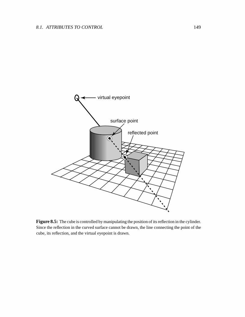
8.1. ATTRIBUTES TO CONTROL 149
virtual eyepoint
surface point
reflected point
Figure 8.5: The cube is controlled by manipulating the position of its reflection in the cylinder.Since the reflection in the curved surface cannot be drawn, the line connecting the point of thecube, its reflection, and the virtual eyepoint is drawn.
150 CHAPTER 8. INTERACTION TECHNIQUES
8.1.7 Free Form Curves and Surfaces
Free-form curves and surfaces are traditionally a difficultproblem for interface design.Typical approaches to creating such objects require devising representations that aresufficiently expressive, are convenient for the user to manipulate directly, and havegood mathematical properties. This typically leads to interfaces like the control pointsof B-Splines, that sacrifice usability. Some of the difficulty stems from the fact that therepresentations also serve as the parameterizations of theobjects. Because of this, itwould seem that the differential approach would be a naturalsolution.
For many types of curve and surface representations, the differential approach canbe applied. For many types of parametric surfaces such as B-splines and NURBS,the positions of points are simple functions of the parameters that can be computed asconnectors and manipulated differentially. Several of theapproaches in the literatureare variants of this, using different schemes for computingparameters changes. Forexample, Welch, Gleicher, and Witkin [WGW91], Welch and Witkin [WW92], Fowler[Fow92], and Hsu et al.[HHK92] all use various constrained optimization techniquesto map manipulation of points on surfaces to the underlying parameters. This permitsthe objects to be manipulated by controlling points on them,rather than control points.In some cases, users may prefer to use control points to manipulate curves or surfaces.Since the positions of the control points can be computed from the curve or surface,control points can be provided even if another representation is used. This allows, forexample, to use Bezier control points to manipulate a B-Spline curve.
Unfortunately, the differential approach of this thesis isinsufficient for adequatelyaddressing the issues in manipulating free form curves and surfaces for many reasons:
� free form objects have too many degrees of freedom;
� free form objects require global control for effective manipulation. Such controlcan be provided only with attributes that compute properties of the entire surface,or large regions of it;
� free form objects often need fine detail local control, requiring adaptive subdivi-sion;
� many of the constraints that are used to sculpt free form objects’ are specializedcases that can be handled more effectively for the large numbers of degrees offreedom.
In short, the methods of this thesis do apply to the manipulation of curves and surfaces,as we showed in [WGW91], but, by themselves, the methods do not address many of thedifficult issues and more specialized methods apply. Controlling free form curves andsurfaces is a very important problem, and is therefore well studied. Some interestingoptimization-based approaches are explored by Celniker and Gossard [CG91] and byWelch and Witkin [WW92] and [WW94].

8.2. STRATEGIES FOR INTERACTION 151
8.2 Strategies for Interaction
The previous section described a large number of attributesthat can be computed andprovided as connectors on objects. With the differential approach, we can control theobjects by attaching controllers to the connectors. In thissection, we consider somestrategies for determining what controllers to attach to which connectors at what time.
8.2.1 Presenting the Abstractions to the User
The most obvious way to employ the differential approach is to provide the abstractionsto the user as directly as possible. At an extreme, the user could be presented with aschematic representation, like the diagrams of Section 1.3.3. While this graph editingapproach has been attempted in systems such as the SPAR Modeling Testbed [FW88],Condor [Kas92] and ThingLab [Bor86], I do not believe it is inthe spirit of directmanipulation, and prefer to hide such representations fromthe user.
The direct application of the differential approach gives the user a palette of con-nectors to which controllers can be applied. Connectors that represent positions canbe controlled by attaching them to the mouse. Non-geometricvalues can be controlledwith sliders or similar widgets. To specify multiple controls, the user might either nailconnectors to their current values, or place goal points forconnectors to seek.
Presenting the abstractions directly to the user has a number of benefits. It permitsthe user to select controls that are applicable to their problem, and to mix and matchcontrols as needed. It maximizes flexibility over what the user can do. Such a directapproach is a useful strategy for testing out new types of controls, as shown in the scenecomposition program of Section 9.7. By utilizing efficient mechanisms for selection, alarge array of attribute types can be provided for control.
The advantages of this direct application are also its most serious problem. Thequestion of how to present the controls to the user can be difficult, especially as thenumber of types that are available grows. The interface musthelp the user understandthe potential choices and to find the controls that are applicable to their task. Whilethe flexibility of a range of controls is useful, it also meansthat a user might needto spend time deciding which control to use and how to employ it. A system mustshow the user what is being controlled and explain the behavior of the objects. Theissues of scalability also arise as the user adds more controls, creating more complicatedbehaviors and worse performance.
One variety of direct application of the differential approach is the “live world.” Alive world is an environment where just about any point can begrabbed and manip-ulated. In such an application, objects, shadows, reflections, lights, or just about anyother entity can be grabbed and dragged. This provides a uniform interface for a widevariety of tasks. However, it still does not solve the problems. A user must be madeaware of what can be dragged and what cannot. Some mechanism for specifying what

152 CHAPTER 8. INTERACTION TECHNIQUES
cursor position feedback
slider handle
persistent target
upper bound mark
lower bound mark
Figure 8.6: A differential slider. Left: feedback shows not only the value specified by speci-fying dragging, but also the actual value of the attached connector. Middle: theGoTowards
controller used to drive the connector toward the specified value can be retained after draggingis completed to nail the value in place. The persistent valueis displayed by the diamond. Right:users can place boundary constraints with the sliders. Upper and lower bounds are displayedas greyed regions.
might change when a point is grabbed is important for controlling things like shadows,where many things might be affected by a single control. Somemechanism for permit-ting the user to specify the desired behavior in under-constrained cases, for example bypermitting grabbable points or objects to be nailed in place, needs to be provided.
Differential Sliders
To present controllers and connectors the user directly there needs to be a mechanismfor controlling any connector output, even ones whose output is simply a dimensionlessscalar value. The mechanism must permit the user to specify the various controllertypes, and provide values for those types that require them.Bramble has a widget calleddifferential sliderthat is a variant of a standard slider designed to control a connectorwith the differential approach. A basic differential slider is shown in Figure 8.6. Betterdesigns that are more self-revealing and easier to use are certainly possible.
A standard slider converts the position of the mouse into a value for its attachedparameter. For the differential approach, such a slider cannot be attached to a con-nector since the value cannot be set directly. To create a basic differential slider, aGoTowards controller is connected to drive the value towards what is specified bythe mouse, rather than directly specifying new values for its attached parameter whendragged. Because the connector’s value may not perfectly track that of the mouse, bothvalues are displayed to the user.
The ability to nail a slider’s value in place is useful feature for a differential slider.

8.2. STRATEGIES FOR INTERACTION 153
Such a facility can be implemented by simply retaining theGoTowards controllerbeyond the completion of the dragging operation. With the Bramble differential slider,this is done by holding a modifier key as the dragging button isreleased. Key pressescan be used to create controllers that drive the slider to itsminimum, maximum, ormiddle value.
A differential slider can be used to apply other controllersas well. For example, theBramble slider can place boundaries on the value by pressingthe third mouse buttoneither above or below the present value. The slider displaysthe current boundaries, asshown in Figure 8.6. Snaps can also be placed on the slider’s value. The slider mustdisplay where the snaps are and provide feedback for when theslider is snapped.
8.2.2 Drawing or Modelling with Constraints
Drawing or modelling with constraints can be seen as a variant of directly providingthe abstractions of the differential approach to the user. In such an approach, a userdeclaratively specifies relationships among parts of the model. Differentially, this en-tails creatingGoTowards controllers for selected attributes that compute the rela-tionships. Often, this is coupled with dragging: the user can drag pieces of the drawingeither by placing and dragging positional constraints, or dragging the model subject tothe constraints.
The idea of using constraints in interactive drawing and modeling dates back toSketchpad[Sut63], the earliest system. Since then, there has been considerable interestin the approach of declaratively specifying parts of the drawing. Some of the advan-tages of the constraint-based approach are:
� the user can specify what is most convenient, in any order;
� the constraints can give structure to the model, potentially embedding the seman-tics of the thing being modelled;
� the constraints can be used to specify exact relationships in the model precisely;
� the constraints are persistent so they maintain previouslyestablished relation-ships to avoid redundant work in reestablishing them after editing.
Many difficult issues have limited the success of constraint-based systems for draw-ing. Not only must a system be able to solve constraint satisfaction problems, but itmust make it easy for users to specify, debug, and edit constrained models. Constraintschange the nature of interaction in a graphical application. Without them, actions onlyaffect the objects to which they refer. For example, dragging an object in a traditionaldrawing program moves only the object. With constraints, this locality is lost: alter-ing one object may cause other objects to be affected. This global nature of constraintoperations is at the core of many of the difficult issues in employing constraints.

154 CHAPTER 8. INTERACTION TECHNIQUES
Without user specified constraints, graphical objects havefixed behaviors. For in-stance, an ellipse in a drawing program behaves like an ellipse. The system designercan design a good, usable behavior which the user can learn and apply to all ellipses.When user specified constraints among objects are introduced, the situation changes.To begin with, the behaviors can become more complicated because of interactionsamong objects. Each combination of objects and constraintswill have its own behav-ior. These behaviors are specified by the user in terms of the constraints; the user iseffectively programming.
As in more traditional programming, complexity in the constrained behavior of agraphical model becomes a problem when it has bugs, e.g. whenthe behavior is notwhat is desired or expected. The most obvious form of bug is when the constraintsforce the model into a configuration that is not what the user desires, or the constraintsprevent the user from achieving a desired configuration. Another class of constraintbug stems from bad constraints where solutions cannot be found, either because ofconflicting specifications or solver failures.
Because constraint errors occur, interactive graphical applications which provideconstraints to users must deal gracefully with bad situations, such as conflicting or re-dundant constraints. Underdetermined models must also be handled, as it is impracticalto expect the user to specify all possible degrees of freedom. Because of the potentialfor errors, it is crucial to aid the user in understanding thecomplex behaviors of con-strained models.
The differential approach helps with some of the issues in creating constraint-basedapplications. Continuous motion facilitates understanding the behavior since users areable to employ their perceptual skills to help understand change. The methods forimplementing the differential approach handle under and over determined cases. Thedynamic implementation of the differential approach can serve as a backbone to pro-viding a constraint-based system where users can experiment with their models in orderto comprehend and debug them.
The Briar drawing program, described in Section 9.1, buildson the differential ap-proach to provide a strategy that addresses other issues in constraint-based tools aswell. By using constraints only to maintain existing relationships during direct manip-ulation, Briar is able to avoid problems with conflicting or unsolvable constraints andunpredictable selection of constraint solutions. A key to making systems like Briar pos-sible is the ability to enforce constraints during continuous-motion, direct-manipulationdragging, as provided by the differential approach.
Although many modern constraint-based systems, such as Briar, show promise inaddressing the issues of the approach, it is not certain thatthe issues can be sufficientlyresolved to become the standard and dominant tools. In particular, issues of scalabilitymay be the ultimate Achilles heel for constraint-based drawing and modelling.

8.2. STRATEGIES FOR INTERACTION 155
8.2.3 Building Interaction Techniques
In the previous sections, we discussed how the abstractionsof the differential approachcan be presented directly to the user. In this section, we consider leaving them in thehands of the interaction technique designer. The idea is to use combinations of con-trols in ways that define desirable behaviors for traditional direct manipulation styleinteractions.
The typical way the differential approach is employed is to use a control to pro-vide interactive dragging, but to define other constraints so the correct behavior oc-curs. Rather than having the user define the constraints, theinterface designer canchoose them. Objects or handles are predefined and can be given carefully designedbehaviors.
For the designer of direct interaction techniques, the differential approach providesa new set of abstractions. The approach can lead to techniques that could not have beenimplemented using traditional techniques. Other times, the abstractions are applied tomore conventional interactions. In fact, most of the examples given later are simplyrecreations of existing interaction techniques. The approach may be most practicalfor prototyping interaction techniques: the technique canbe designed using the toolsof the differential approach, permitting it to be quickly defined and evaluated. Thenthe mathematics can be re-derived to compile the interaction technique into a moretraditional implementation.
Because controls are used in predefined combinations, many of the most seriousdrawbacks of the differential approach and constraint-based systems are avoided:
� the number of controls is a small constant that does not grow as the model be-comes larger;
� the combination of controls can be checked to insure that they are well behavedbefore being handed to users;
� the behavior of objects is explicitly designed, rather thanjust coming about as abyproduct of placing constraints. This can leave the specification of interactivebehaviors in the hands of the “trained professionals.”
Many of the same arguments are given for the design of the Siriconstraint-based pro-gramming language [Hor93]. Siri uses constraint techniques within objects to helpdefine their behavior, but uses more conventional methods for inter-object communi-cation.
There are two main ways that the differential approach is used for defining inter-active behaviors. One is to define types of objects that behave as desired. The other isto define handles that have particular functionality. This latter, more common categorytypically involves creating a number of constraints in addition to the mouse attachmentduring a dragging operation. Many examples are given later in this chapter.

156 CHAPTER 8. INTERACTION TECHNIQUES
Figure 8.7: A 3D image overlaid on top of a corresponding real image. Our goal is to placethe virtual plant on the real table. In each image, there is a table (denoted by the white rectanglefor the graphics image). Initially, the images do not correspond because the virtual camera isnot in the same place as the camera used to create the real image.
To define the behavior of a object that will be manipulated using the traditionaldirect manipulation interface of dragging the position of asingle point at a time, thedifferential approach offers advantages. First, constraints can be used internal to theobject to define relationships that must be maintained as theobject is dragged. Sec-ondly, by providing a way to implement the dragging, it spares the object designer theeffort of mapping from position values to parameter values.It also permits a uniformmechanism to be used to drag all points on all objects.
8.2.4 A Concrete Example: Aligning a Camera to an Image
We now consider a very specific interaction technique as an example, and discuss howit can fit in with the strategies of this section. The problem is to align a synthetic imageof a 3D scene with a real image by configuring the virtual camera creating the syntheticimage. We assume that both the real scene and the synthetic scene each have a table ofidentical size in them. An example is shown in Figure 8.7.
With through-the-lens controls and the differential approach, the correspondenceproblem can be solved easily. Through-the-lens controls are used to drag the cornersof the virtual table to their corresponding positions in theimage, causing the camera tobe moved. Each control is locked as it is placed. Manipulating the positions of the fourcorners of the table causes the virtual camera to be placed ina position where the two

8.2. STRATEGIES FOR INTERACTION 157
Figure 8.8: The synthetic and real images are registered by successively dragging the cornersof the table to their corresponding positions in the image.
images correspond. This process is shown in Figure 8.8.
The registration task is an excellent example of the benefitsof the differential ap-proach. It solves an important and useful task that would be extremely difficult withtraditional interaction techniques. In order to define the interaction technique withoutthe differential approach, the mathematics to determine the camera configuration fromthe corners of the rectangle would have to be derived. While such a derivation is possi-ble, it would be extremely difficult to do in a robust manner asit is an overdeterminedproblem. With the differential approach, it is a straightforward combination of four 2Dpoint controls. The method over-determines the solution, specifying eight controls fora camera which has only seven degrees of freedom. However, the methods of Chapter3 can handle these over-determined cases.
The table registration required the use of four through-the-lens point controls. Thosecontrols could have been specified either by the user, or by aninteraction techniquedesigner building a mechanism for the particular task of image registration. If the ab-stractions of the differential approach were directly provided to the user, the registrationtask would require the user to freeze the position of the table in the world, enable thecamera to be controlled, select through-the-lens positioncontrols for each corner of thetable, and then drag these controls. In a more constraint-based interface style, theremight be a command for dragging points with through the lens controls, which the usercould successively apply to each corner of the table.
Because image registration is an important task, an interaction technique designermight want design an interface for it. For example, the designer might create the virtualtable as a special object that when its corners are grabbed, the system knows to applya through-the-lens control on the point to manipulate the camera, and to leave thesecontrols locked in place even after they’ve been manipulated. The user would see acommand to create the alignment table, and would directly manipulate table corners,but the abstractions of the differential approach would be hidden, serving simply as atool for the interaction technique designer.

158 CHAPTER 8. INTERACTION TECHNIQUES
8.3 Sources of Constraints
The basic idea behind each of the strategies of the previous section is to provide con-straints so that manipulation operations like dragging have the desired effects. Themajor difference in the strategies is how these constraintswere specified, whether theywere provided by the interaction technique designer or by the user. In this section, weconsider what constraints can be useful for manipulation, and how they are used in con-junction with dragging to create interaction techniques. This section is organized by“sources” of constraints, the kinds of things that specify constraints on manipulation.
The general problem in manipulation will be to handle the underdetermined natureof dragging. Our input devices will undoubtedly specify farfewer degrees of freedomthan the model contains, or even than typical objects contain. For example we mightcontrol an articulated figure with a 6 degree of freedom tracker or control a 3D positionwith a mouse.
The large number of degrees of freedom problem is especiallyimportant in 3Dmanipulation. Unlike in the real world, the objects we manipulate with a 3D user in-terface can float freely in space, and therefore have extra degrees of freedom. Theproblem of 3D manipulation is to somehow control these degrees of freedom with thelimited input devices we have. One approach to this problem is to develop better inputdevices. For the work in this thesis, I have considered only the mouse. However, thedifferential approach is input-device-independent, and even with better input devices,the constraint-based approach applies – in the real world westill use constraints formanipulation even with our dextrous hands.
When we encounter an object with many degrees of freedom in thereal world weemploy a variety of tactics to manipulate it. We use manipulators in parallel, for ex-ample by coordinating our hands or fingers, or we create constraints, either by using anextra hand or finger or by using interactions between objects. For example, we mightturn 3D problems into a 2D one by placing the objects on a flat surface, or for morecomplex manipulations we might build a jig to limit the objects’ behaviors to make iteasier to achieve the desired manipulations.
However, we normally design our objects so that they don’t have as many degreesof freedom. The behaviors of most objects we manipulate are constrained by theirrelationships with other objects or their structure constrains them to move only in thecorrect fashion. For example, operating a door requires only one degree of freedom(its hinge) or two (its knob and hinge) and car steering wheels and levers rotate only inuseful ways.
These real world tactics for manipulation all rely on constraints on object motion tosimplify the manipulation problem. The sources of these constraints vary: they comefrom the mechanical structure of the object, interactions among objects, conventionson the uses of objects, or from other hands or fingers. In this section, we will use thesame approach to address the problem of manipulation in interfaces. The general idea

8.3. SOURCES OF CONSTRAINTS 159
for creating an interaction technique will be to provide a sufficient set of constraints sothat control of a single point defines a desired behavior. Fordefining 3D interactiontechniques using the mouse, we will attempt to define a sufficient set of constraints sothat the two degrees of freedom specified by a through-the-lens control are sufficientto control the 3D object.
8.3.1 Intrinsically Constrained Problems
For some manipulation tasks, the object being manipulated is intrinsically constrainedsufficiently. For example, even in a 3D world, dragging a point along a fixed plane,such as the floor, is a 2D problem. So, if a point is by definitionin a fixed plane, it issufficiently constrained so that a 2D input device can be usedto control it. An exampleof such a point would be shadows on the floor. This is part of thereason for the interestin shadow manipulation.
8.3.2 Artificial Constraints
A common way to create interactions is to create synthetic constraints based on someuser command. For example, based on the state of a modifier keyor a command mode,the system might constrain object motions to rotate about a particular axis or translatein a particular direction.
An example 3D interaction technique using artificial constraints is the mousepole,introduced in Section 7.8. The mousepole allows the user to position a point in 3Dusing the mouse by constraining the point to lie in the plane parallel to the ground. Theray cast from the mouse position defines a unique point on thisplane. Depressing abutton switches the mousepole to operate in a plane perpendicular to the ground. Wedraw a vertical pole from the point to the ground in order to indicate height, hence thename mousepole.
The advantages of these artificial constraints are that theycan be applied to anyobject and are easy to create. However, it is easy to make suchinterfaces complicatedby including large numbers of modes, modifier keys, and commands. It can be difficultto make such interfaces self-revealing. Using a standard ofartificial constraints on allobjects has the advantage of uniformity, but has the problemthat it does not permitobjects to special behavior.
8.3.3 Object Semantic Constraints
The graphical objects that we manipulate often have structure or semantics that maydictate how they should behave when manipulated. This behavior can often be ex-pressed as constraints, sometimes corresponding to the mechanical structure of the ob-ject, and sometimes to the intended purpose or conventions of use of the objects. For

160 CHAPTER 8. INTERACTION TECHNIQUES
example, the Luxo lamp of the introduction has many pieces each with many degreesof freedom. However, the mechanical structure of the lamp significantly reduces thedegrees of freedom in the lamp, making it much easier to control.
Many of the objects we must manipulate have only a few degreesof freedom: use-less motions are constrained away. There are many example ofobjects whose behavioris sufficiently constrained so that one or two controls are sufficient, for example, steer-ing wheels, airplane yokes, doors, levers, or the handle of aslot machine. There aresome implied assumptions in these manipulations, for example when the handle of aslot machine is grabbed, we assume that we are attempting to pull the lever, not movethe machine.
Sometimes, the constraints on objects stem not from the objects’ mechanical struc-ture, but rather from conventions on how they are used. For example in moving a pieceof furniture, we are most typically interested in sliding italong the floor or turning it,not necessarily lifting it or flipping it over. In such cases,it is conceivable to buildinterfaces which imbue the objects with the constraints that cause the more commonbehavior, and require some less direct method for other manipulations. In analogy tothe real world, I can push the furniture around on my floor, butto lift it or flip it, I needto get some extra help. The desire to perform non-standard manipulations also existsfor mechanically constrained objects, for example, we might want to rip the head offthe Luxo lamp.
Often, the manipulation task provides sufficient information to adequately constrainobjects so that simple point manipulations suffice. For example, positioning a pictureon a wall or a lamp on a desk are both 2D problems. Pulling the arm of a slot ma-chine is a one dimensional problem if the model behaves like aslot machine. I callthe strategy of attempting to use the natural constraints ofthe task to create interactiontechniquesmanipulation from structure.Such constraints are called “context specificconstraints” by [Hou92]. These constraints that arise fromthe structure of the modelare advantageous because they only restrict the user from performing operations whichare typically undesirable, they are often already inherentin the parameterization of themodel, and they are easily understood by the user.
There are many issues in employing manipulation from structure in realistic sys-tems. For one, it requires that the system have some knowledge of what the objectsare, and how they should behave — a collection of polygons might look like a paintingwhich should remain hung on a wall to the user, but the system must not only knowhow paintings are to behave, but also how to identify them. The structure of the modelmust be created in a manner that has the proper semantics. Whenmanipulating suchmodels, it can be difficult to know if the model is sufficientlyconstrained such that2D manipulations will provide enough control. While the differential approach doesnot directly address these problems, it does make it far easier to explore manipulationfrom structure by providing a vocabulary with which the semantic constraints can beexpressed and by mapping controls to whatever parameters are used to represent the

8.3. SOURCES OF CONSTRAINTS 161
models.
8.3.4 Handles
Handles are particular points associated with objects thatcan be grabbed. Handles areoften given specific meanings as to the manipulation that they perform. For example,in a typical Macintosh direct manipulation interface, a graphical object has particularhandles that cause it to be scaled.
Handle behavior can be defined by associating each handle with a set of constraintsthat are applied to the object as the object is manipulated. For example, to create theMacintosh-style scale handles, the position of the opposite corner of the object mustbe pinned down while the handle is dragged. Bramble’s grab and ungrab hooks werespecifically designed to help define handle behaviors with constraints.
8.3.5 Widgets
Although building the constraints required for manipulation into each graphical ob-ject has many attractions, it does have some serious drawbacks. Most obvious is thatbehavior must be built into each object, and that each objectmust have sufficientlywell-designed behavior so that it is manipulable and that the constraints are apparentto the user.
An alternative to giving every object a behavior is to define special objects whichhave behaviors and to manipulate the other objects by attaching them to thesewidgets2.These widget objects can be specially designed to have desirable and self-revealingbehaviors. A widget can be thought of as a tool for providing aspecific type of ma-nipulation. Widgets have become ubiquitous in graphical interfaces. Most graphicaluser interfaces now have users specifying values with widgets such as sliders, dials,and buttons.
With the differential approach, connections are bidirectional. If a widget displays avalue, it can also serve to control the value. The functions that map from the screen po-sition of the input device to the values stored by the widget do not need to be provided,only the forward direction functions required for drawing.This is exemplified in thefuel gauge widget example shown in Figure 8.9. The complete code for this exampleis presented in Section A.2.1, but a simplified version is defined using the Brambledefine-shape function:
2The definition of widget here is slightly different than thatof [CSH+92]
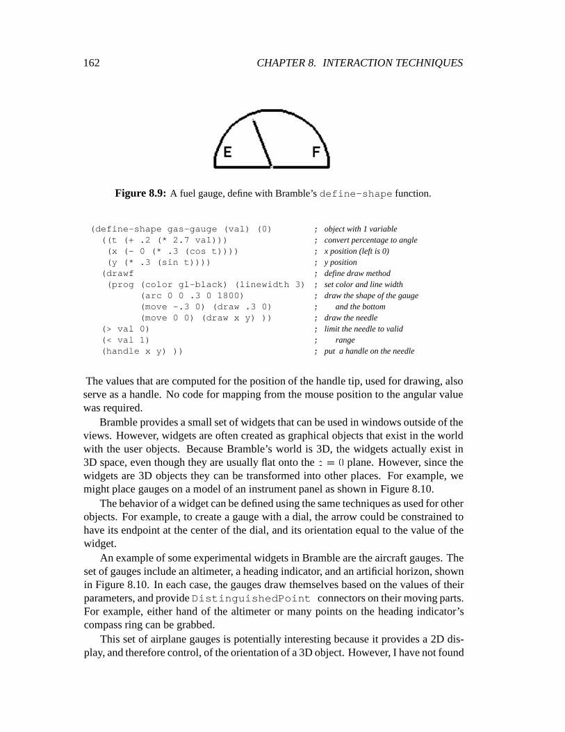
162 CHAPTER 8. INTERACTION TECHNIQUES
Figure 8.9: A fuel gauge, define with Bramble’sdefine-shape function.
(define-shape gas-gauge (val) (0) ((t (+ .2 (* 2.7 val))) (x (- 0 (* .3 (cos t)))) (y (* .3 (sin t)))) (drawf (prog (color gl-black) (linewidth 3) (arc 0 0 .3 0 1800) (move -.3 0) (draw .3 0) (move 0 0) (draw x y) )) (> val 0) (< val 1) (handle x y) ))
; object with 1 variable; convert percentage to angle; x position (left is 0); y position; define draw method; set color and line width; draw the shape of the gauge; and the bottom; draw the needle; limit the needle to valid; range; put a handle on the needle
The values that are computed for the position of the handle tip, used for drawing, alsoserve as a handle. No code for mapping from the mouse positionto the angular valuewas required.
Bramble provides a small set of widgets that can be used in windows outside of theviews. However, widgets are often created as graphical objects that exist in the worldwith the user objects. Because Bramble’s world is 3D, the widgets actually exist in3D space, even though they are usually flat onto thez = 0 plane. However, since thewidgets are 3D objects they can be transformed into other places. For example, wemight place gauges on a model of an instrument panel as shown in Figure 8.10.
The behavior of a widget can be defined using the same techniques as used for otherobjects. For example, to create a gauge with a dial, the arrowcould be constrained tohave its endpoint at the center of the dial, and its orientation equal to the value of thewidget.
An example of some experimental widgets in Bramble are the aircraft gauges. Theset of gauges include an altimeter, a heading indicator, andan artificial horizon, shownin Figure 8.10. In each case, the gauges draw themselves based on the values of theirparameters, and provideDistinguishedPoint connectors on their moving parts.For example, either hand of the altimeter or many points on the heading indicator’scompass ring can be grabbed.
This set of airplane gauges is potentially interesting because it provides a 2D dis-play, and therefore control, of the orientation of a 3D object. However, I have not found

8.3. SOURCES OF CONSTRAINTS 163
Figure 8.10: Gauges serve as both displays and controls of the plane’s configuration. Al-though they are 2D objects, the gauges can be placed anywherein the 3D scene.
the airplane gauges to be a useful interaction technique forcontrolling 3D objects.
8.3.6 3D Widgets
Traditional 2D widgets can be applied to 3D interfaces. To avoid the drawbacks of suchan approach, [CSH+92] introduces the notion of 3D widgets as tools in the object’sspace.
The differential approach offers a mechanism for defining the behavior of 3D wid-gets, which is a central difficulty in their design[ZHR+93]. With our approach, wedefine the behavior of a 3D widget with a set of constraints that sufficiently restrict itsbehavior so that a through-the-lens control can be used. These constraints are appliedwhile the widget is operated.
Figure 8.11 shows some example 3D widgets modelled after theones presented in[CSH+92] and [SC92]. The “jack” widget on the left is used to translate an object alongan axis. Pulling a tip of the jack causes the widget and its attached object to move inthe direction shown by the arrow. When a handle is grabbed by pressing the mousebutton, the object is constrained so it can only translate along the axis, and a through-the-lens control is applied to the handle. When the mouse is released, the constraintsare removed. Similar techniques are used to create widgets for rotation about a pointor axis, or to scale either uniformly or along an axis. Bettergraphic design can makethe widgets more self-revealing.
Widgets to control the viewpoint, such as a virtual sphere, can also be created withthe differential approach. The exact virtual sphere technique of [CMS88] is harder tocreate using the building blocks provided because the sphere that the user grabs is inscreen space, rather than in object space. This has a number of disadvantages as it losesthe kinesthetic coupling between dragging and the visible behavior. The arcball methodof [Sho92] makes this problem worse by introducing a scalingfactor to simplify the
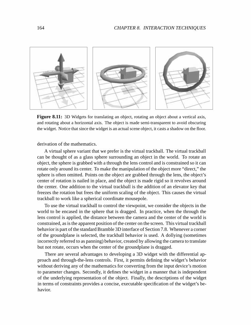
164 CHAPTER 8. INTERACTION TECHNIQUES
Figure 8.11: 3D Widgets for translating an object, rotating an object about a vertical axis,and rotating about a horizontal axis. The object is made semi-transparent to avoid obscuringthe widget. Notice that since the widget is an actual scene object, it casts a shadow on the floor.
derivation of the mathematics.
A virtual sphere variant that we prefer is the virtual trackball. The virtual trackballcan be thought of as a glass sphere surrounding an object in the world. To rotate anobject, the sphere is grabbed with a through the lens controland is constrained so it canrotate only around its center. To make the manipulation of the object more “direct,” thesphere is often omitted. Points on the object are grabbed through the lens, the object’scenter of rotation is nailed in place, and the object is made rigid so it revolves aroundthe center. One addition to the virtual trackball is the addition of an elevator key thatfreezes the rotation but frees the uniform scaling of the object. This causes the virtualtrackball to work like a spherical coordinate mousepole.
To use the virtual trackball to control the viewpoint, we consider the objects in theworld to be encased in the sphere that is dragged. In practice, when the through thelens control is applied, the distance between the camera andthe center of the world isconstrained, as is the apparent position of the center on thescreen. This virtual trackballbehavior is part of the standard Bramble 3D interface of Section 7.8. Whenever a cornerof the groundplane is selected, the trackball behavior is used. A dollying (sometimesincorrectly referred to as panning) behavior, created by allowing the camera to translatebut not rotate, occurs when the center of the groundplane is dragged.
There are several advantages to developing a 3D widget with the differential ap-proach and through-the-lens controls. First, it permits defining the widget’s behaviorwithout deriving any of the mathematics for converting fromthe input device’s motionto parameter changes. Secondly, it defines the widget in a manner that is independentof the underlying representation of the object. Finally, the descriptions of the widgetin terms of constraints provides a concise, executable specification of the widget’s be-havior.
8.3. SOURCES OF CONSTRAINTS 165
8.3.7 Discussion
The differential approach lets us define and implement a variety of strategies for ma-nipulating objects. The strategies are not mutually exclusive, for example we mightattach a widget to a part of a constrained object (particularly if it is not sufficientlyconstrained) or use modifier keys to alter the behavior of a widget. As we experimentwith different strategies, we find that they all have advantages and drawbacks. Here,we discuss some considerations.
User provided vs. designer provided: Making the user responsible for providingconstraints may give the user more flexibility, but might also make them expend moreeffort as they specify behavior in addition to geometry. It also exposes them to the rangeof problems inherent in specifying behavior. Interface designers are (hopefully) betterat devising good interactive behaviors, but cannot tailor designs to specific operations.If the objects to be manipulated will be used often, or replicated many times, it becomesworthwhile to spend effort in building behavior into them. This might be done by theuser, the interface designer, or by someone else who is simply an object designer.
Smart objects vs. smart tools: Do we put lots of behavior into the objects, so thatthey can be manipulated with simpler tools, or do we develop better tools so that ourobjects need less behavior? An extreme case of the former would be an interface whereevery object had sufficiently well defined behavior so that any point could simply begrabbed with a though-the-lens control. An extreme case of the latter would be tohave uniformly simple objects, for example ones that are being subject to the standardtranslate, rotate, scale transformations, and provide a set of widgets or commands whichoperate on them.
Context-sensitive vs. context-free: Is object behavior uniform, or do different ob-jects (or even parts of objects) behave differently? Tailoring behaviors to objects hasadvantages, as discussed by [Hou92], but uniformity does too.
Bounded scope vs. unlimited connection: Permitting arbitrary relationships amongobjects can simplify manipulation by restricting unwantedbehaviors, but when manyobjects interact, their coordinated behaviors become complicated as longer chains ofcausality are possible. Strategies which manipulate single (or a small number of) ob-jects, such as widgets, have the advantage of keeping their simple behavior as the en-vironment scales, but may grow tedious to use as the user mustconsider an increasingnumber of objects and interactions.

166 CHAPTER 8. INTERACTION TECHNIQUES
8.4 Employing Switching
In Section 6.4, controllers that operated by switching simpler controllers on and offwere presented. In this section, we examine how these switching controller might beused.
8.4.1 Generalized Snapping
In Section 6.4.2, a controller for snapping to values was developed to aid in providingaccurate direct manipulation. TheSnap controller causes a connector to be driven to aparticular value when it approaches that value. Because thecontroller can be attachedto any connector, it provides a general method of snapping and its use is, therefore,referred to as generalized snapping.
Generalized snapping can be used to recreate the typical cursor snapping by repre-senting the cursor as a differentially controlled object and creatingSnap controllersthat drive it towards desired snap targets.
Other behaviors can be created by placingSnap controllers on connectors otherthan those that are being directly manipulated. Because controller handling happensasynchronously in parallel with manipulation, precise relationships can be establishedaway from where the cursor is. For example, if users often desire line segments to beaccurately vertical, that is when something appears vertical it should be vertical,Snapcontrollers for the values�=4 and3�=4 can be placed on the angle connectors of eachline segment. If a line segment is brought near being vertical as it is dragged, the con-figuration of the line segment would “snap” to a configurationwhere it was vertical.While this small jump may violate the continuous motion, it isusually small and pre-dictable enough that it is permissible, especially when proper feedback is provided toexpress what snapping operation has occurred.
With generalized snapping, the snapping can occur away fromthe dragging action.For example, if the line segment of the preceding paragraph was attached to some link-age mechanism, the user might be controlling the line segment by manipulating someother part of the mechanism, as shown in Figure 8.12. This makes it even more crucialto provide proper feedback to the user to denote when something is snapped. Becausethe focus of attention is possibly away from the snap, for example at the dragging site,auditory cues might be useful as well.
The generalized snapping technique has many drawbacks thatneed to be resolved.First, it does not revert objects to their original configuration when unsnapped. Sec-ondly, it needs to be connected to mechanisms that handle multiple snap targets. To dothis properly might require the ability to determine whether two constraints conflict.Third, because the differential approach only drives connectors towards particular val-ues, there is no guarantee that the snap controller accurately reaches its target. Finally,the snap controller has a number of potentially sensitive parameters that must be fine-

8.4. EMPLOYING SWITCHING 167
Figure 8.12: Generalized snapping can occur away from the dragging action. As the userdrags the linkage mechanism, the left line segment gets snapped to the vertical position. Be-cause such snapping can take place away from the focus of attention, it is important to provideproper feedback.
tuned to provide the correct “feel.”
8.4.2 Collisions
Non-interpenetration is a useful constraint on objects. Such a constraint causes objectsto collide and contact one another when they touch, rather than to simply pass through.A collision is the initial impact between two objects, whichmay remain in contact withone another afterwards.
With the differential approach, it is possible to create non-interpenetration con-straints using inequalities. While the methods are not as sophisticated as the specialpurpose collision simulation methods reviewed in Section 2.2.3, they are simple tobuild with the abstractions of the differential approach, and are sufficiently effective tobe interesting.
A particularly simple case of collision avoidance is used inbox-and-arrow diagramcreation, an application discussed in Section 9.3. The particular constraint we wouldlike to enforce is that two axis-aligned rectangles do not overlap. This can be expressedas a disjunction: if at least one of the following inequalities hold, then the rectanglesdo not overlap:
x
1
+ s
x
< x
2
� s
x
(8.10)
x
1
� s
x
> x
2
+ s
x
y
1
+ s
y
< y
2
� s
y
168 CHAPTER 8. INTERACTION TECHNIQUES
y
1
� s
y
> y
2
+ s
y
;
wherex andy are the coordinates of the center of each rectangle, ands is the size. Eachclause represents one of the possible ways for the rectangles to be separated, either 1 isabove 2, below 2, left of 2, or right of 2. Alternatively, the disjunction can be expressedas a maximum operation of the four terms.
The differential approach permits conjunctions of constraints to be handled easily,however disjunctions are more difficult. Enforcing the disjunction is not a problemwhen it is true, as each term can be checked until one that is true is found. However,when none of the expressions of the disjunction is true, a choice must be made. As withinequalities, when the constraint is violated it will be activated in order to “pull” it backto the admissible region. In the case of the disjunction, at least one of the expressionsmust be chosen and used as a constraint. Even though all of theinequalities are violated,all cannot be enabled because they would conflict.
The strategy for handling disjunctions of inequalities will be to select one of theinequalities to enable when the disjunction is violated. Because we are not backingup the instant where the disjunction began to fail (see Section 6.4.5), we must resortto enabling a violated inequality and permitting it to pull the configuration back to alegal configuration. The difficulty is selecting the inequality, which must be done bya heuristic. Although we would like to pull things out the same way they went in, thelack of history makes it impossible to do exactly.
A heuristic used for the simple rectangle overlap problem isto pick the inequalitythat is least violated. This technique is used for object non-overlap in the box andarrow diagram editor program of Section 9.3. The heuristic fails in two cases depictedin Figure 8.13. First, if the overlap is near a corner, an object may be pushed out tothe side, rather than the way that it came in. Second, if the ODE solver step moves theobject too far through the second object, it might be closer for the object to push outthe opposite side that it came in from.
The basic rectangle non-overlap can be extended to the general case of rigid (e.g.rotatable) convex polygons. The basic element of a non-overlap constraint for two suchobjects is a point outside of polygon constraint. This is created by a disjunction, theremust be at least one edge of the polygon that the point’s distance inside the half-planedefined by the edge is positive. A point outside polygon constraint can be created witha similar heuristic as the rectangle non-overlap, with similar selection problems.
Two convex polygons do not overlap if and only if all the points on each are outsideof the other. This makes it easy to break the polygon collision problem into point out-side of polygon problems. What a polygon collider must do is find points that are insidethe other polygon, called contact points, and enable constraints to push them outside.It will always be sufficient to choose at most two contact points, as this will establisha dividing edge between the polygons. After being selected,each of the contact pointschooses an edge to be pulled out through. The heuristic must make sure that the pointsboth exit through the same edge, even if they are on differentobjects.

8.4. EMPLOYING SWITCHING 169
1
2
3
1
2
3
Figure 8.13: A disjunction of inequalities constrains two axis-alignedrectangles from over-lapping. Because the selection of a direction to pull the block out is made without knowledgeof the direction it came in, two types of errors may be caused.If the overlap is in a corner, thedistance out the side may be less than the distance back out the top, as shown in the sequenceon the left. Also, if the object moves too quickly it may pass through the other object, as shownin the sequence on the right.

170 CHAPTER 8. INTERACTION TECHNIQUES
Figure 8.14: Mechanisms that can simulated using the simple collisions methods of the dif-ferential approach. The left shows a set of sawtooth “gears”jammed with a square block, andthe right shows a block feeder.
While this simple method for collisions is not perfect, it is extremely simple to im-plement, and achieves good enough performance to allow someinteresting mechanismsto be created with it. Two examples are shown in Figure 8.14. Since these methodswere developed, techniques to permit robust simulation of collisions interactively havebeen developed by David Baraff [Bar94].

Chapter 9
The philosopher’s have, in many ways, tried to interpretthe World. The point, however, is to change it.
— Karl Marx11th thesis on Feurbach
Example Applications
This chapter describes some sample applications built withthe differential approachand the tools developed in the previous chapters. The purpose of discussing these ap-plications is threefold:
� to show how the interaction techniques developed with the differential approachcan be fit in the context of a realistic application.
� to show that the differential approach is viable.
� to show some of the range of the tools, particularly the Bramble toolkit, givingevidence of how the differential approach can be used to makesuch tools moregeneral.
All of the example applications discussed, except for the Briar drawing program,were constructed using the Bramble toolkit.
9.1 A Drawing Program
Although constraint-based techniques have been used sinceSketchpad [Sut63], the ear-liest drawing program, they have not been generally successful. Many difficult issueshave limited the success of constraint-based systems for drawing. Not only must asystem be able to solve constraint satisfaction problems, but it must make it easy forusers to specify, debug, and edit constrained models. TheBriar1 drawing program at-tempts to address all of these issues. The issues of constraint-based drawing that Briaraddresses apply more generally to interfaces built with thedifferential approach. Briaris discussed in detail in [GW94] and [Gle92a], and illustrated in Figure 9.1.
A major goal in the development of Briar was to build a system with constraintsthat provided users with the fluent interface that they have come to expect from direct
1It is called Briar because, like the plant it is named for, things stick together inside of it.
171

172 CHAPTER 9. EXAMPLE APPLICATIONS
D
T
BG O
0
V 90
M rule
H 0.25
A 0.75
Figure 9.1: Briar editing a constrained drawing.

9.1. A DRAWING PROGRAM 173
manipulation drawing programs. The techniques in Briar aimto add at least some of theadvantages of constraints without detracting from what hasmade direct manipulationdrawing programs so successful. In short, they aim to make Briar a direct manipulationdrawing program augmented with constraints, not a drawing program with a primar-ily constraint-based interface. The interface feels similar to other direct manipulationdrawing programs which provide snapping except that once snapped, things can sticktogether.
The basic idea behind Briar is to enhance an existing, successful, direct-manipulationdrawing technique with constraints. Briar separates the task of initially establishingrelationships in drawings from that of maintaining them during subsequent editing.It uses snap-dragging, a successful non-constraint-basedtechnique introduced in Gar-goyle [BS86], for initially establishing relationships indrawings. By augmenting snap-dragging, Briar obtains the constraint specification with little or no additional effortfrom the user. The methods of the differential approach allow the constrained draw-ings to be be manipulated directly; as the user drags an object, constraint techniquesadjust other objects to maintain relationships.
Combining snap-dragging with constraint techniques significantly changes the na-ture of the constraints. Unlike most previous constraint-based approaches that rely onsolving methods to initially satisfy the relationships, constraint methods in Briar areused only to maintain relationships during dragging. This permits using the differ-ential approach, as objects move only during continuous-motion dragging. The pri-mary benefits of using constraints only to maintain constraints during dragging parallelthose that motivated the differential approach in Section 1.2: we can avoid solvingnon-linear equations from arbitrary starting points; we need not select configurationsin under-constrained cases, and we can aid the user in the problem of understandingstate transitions by always providing continuous motion.
In Section 8.2.2 discusses many of the challenges in creating constraint-based draw-ing editors. The differential approach addresses some of these. Briar includes tech-niques designed to address many others including how to specify constraints, how toedit them, and how to display them to the user. These issues arise in a wide range ofapplications. This section describes Briar in detail to illustrate some possible solutionsto these problems.
9.1.1 Augmented Drawing Tools
Briar’s approach only uses constraint techniques after relationships are already estab-lished. To establish the relationships initially, we use techniques such as grids, gravity,and snap-dragging [BS86] that have been employed by non-constraint based drawingprograms. To avoid giving the user the extra work of specifying both the constraintsand an initial solution, Briar providesaugmented snap-dragging.Augmented snap-dragging is a variant of snap-dragging that has been extended to specify persistent con-

174 CHAPTER 9. EXAMPLE APPLICATIONS
straints as well as positions. The basic idea is that the cursor placement operations ofsnap-dragging contain information about why an object was positioned where it was,and therefore they can also provide a constraint specification in addition to positionalinformation. The technique can also aid traditional constraint-based drawing programswhich require good starting points to prevent long jumps that are hard for solvers tomake and users to understand.
Ours is not the first attempt to spare users from additional effort required to explic-itly specify constraints. Previous systems have attemptedto infer relationships afterdrawing operations by looking at the resulting drawing, as in automatic beautification[PW85], sequences of drawings, as in Chimera’s snapshot mechanism [KF93], or at atrace of user actions, as in Metamouse [MKW89]. Because this information typicallydoes not specify the relationships unambiguously, these systems relied on heuristicsor asked the user to resolve the ambiguity, as in Peridot [MB86] and Druid [SKN90].Our approach provides positioning methods which unambiguously specify constraints,eliminating the need for inferences. We simply augment drawing tools to specify con-straints as well.
In Briar, augmented snap-dragging is the only method for specifying constraints. Itprovides a uniform method for creating a variety of constraints, such as controlling dis-tances, positions and orientations. Other systems which infer constraints from snappingeither have a limited vocabulary of constraints, such as theManhattan gridding rulesof the interface builder of [HY91], or use other methods to specify the complete setof constraints, as in Intellidraw [Ald92] and DesignView [Com92]. Rockit [KLW92]also infers gridding constraints from drawing actions, butdoes not avoid ambiguity, ac-tually averaging multiple possibilities. Chimera [Kur93]has both snap-dragging andconstraints, but does not integrate the two.
Here is the basic idea behind snap-dragging. When drawing, itis difficult to posi-tion a pencil precisely without using some form of aid. Similarly, it is difficult to drawprecisely with a mouse or other pointing device unaided. Computer software can pro-vide tools for precise placement by drawing from a software-positioned cursor2 ratherthan using the pointing device location. The software cursor’s location is influenced bythe position of the pointing device, but determined by a function which helps the userposition elements precisely.
The uniform grid is the most common function for mapping pointer location to cur-sor position. It displaces the cursor to points on an equallyspaced rectangular grid.“Gravity” is another cursor positioning function. When the pointer is brought suffi-ciently close to an interesting element in the scene, the cursor snaps to it. The idea ofgravity has existed for a long time, having been demonstrated as early as Sketchpad[Sut63]. snap-dragging [Bie89, BS86] enhances the usefulness of gravity. The cursorsnaps not only to the edges of objects, but also to interesting points in the scene such
2This differs from the original snap-dragging terminology [Bie89] where the position of the hardwarepointing device is known as the cursor and the software cursor is known as the caret.
9.1. A DRAWING PROGRAM 175
as intersections and vertices of objects. The ability to snap to intersections enables theuse of traditional drafting compass-and-straight edge constructions.
Since cursor placement operations contain information about why an object waspositioned where it was, they can also provide a constraint specification. Suppose theuser, while dragging an object, moves the pointer near another object so that the cursor,and the point being dragged, snap to the second object. This may have been an accident,but the user might have been trying to achieve this relationship. We provide the userwith the option of making the relationship persistent, so ifit was intentional it can bepreserved during subsequent editing. We call the extensionof snapping to specify arelationship in addition to a positionaugmented snapping.
When a new relationship is established by snapping, the system acknowledges it bydisplaying a symbol indicating the constraints that the snapping operation implies. Theuser can accept the new constraint, by pressing a key to make it persistent, or ignoreit. If this automatic constraint generation process works well, the user will want toaccept most constraints so the option of making this the default should be provided.3
In such a mode, it must be easy for the user to reject an action as an accident. In Briar,a key is used to toggle new relationships between the accepted state, in which they aremade into persistent constraints, and the ignore state, in which the symbols are removedbefore the next drawing operation begins.
Snap-Dragging provides two basic operations for positioning points in two dimen-sions: snapping the cursor to a point, such as a vertex, and snapping the cursor to anobject’s edge or curve. These operations correspond directly to the constraints “points–coincident” and “point–on–object” respectively. The two constraint types work witheach object type that Briar supports. The set of objects presently includes lines, circles,ellipses, and rectangles.
Relations other than contact are created in snap-dragging throughalignment ob-jects: objects that are not part of the drawingper se,but exist only to be snapped to.The original snap-dragging work includes several types of alignment objects, each cor-responding to types of relationships which are useful in drawings. For example, thedistance from a point can be specified by placing an alignmentcircle around that point.Other alignment objects include slope lines, angle lines, and distance lines. The use-fulness of alignment objects is further enhanced by making them easy to place. In fact,heuristics can often automatically place alignment objects where needed.
The two simple snapping operations combined with alignmentobjects allow a userto establish a wide variety of relationships. The simple mapping from snaps to con-straints extends to a variety of constraints. For instance,snapping to an intersection isa conjunction of the simpler constraints. By using the simple constraints with alignmentobjects, the relationships specified by snapping to these objects can be made persistent.For example distance-from-point constraints are created by snapping to an alignmentcircle. The Gargoyle editor [Bie89] shows how snap-dragging can be used to create
3In our experience, the automatic constraint generation is so good that we make it the default.

176 CHAPTER 9. EXAMPLE APPLICATIONS
(a) (b)
(c) (d)
(e) (f)
Figure 9.2: Feedback mechanisms display exactly what is snapped to. Thecursor changesshape depending on whether it is snapped to a curve or edge (a,b), or a point such as an endpointor intersection (c,d). The object snapped to is brightly lit. If several objects are close together,the one desired can be selected by cycling (e,f). Color is used for feedback when available.
most of the relationships which are needed in drawings. Augmented snap-draggingextends this to inferring a similarly complete set of constraints.
Hidden state is a fundamental problem in the interface between man and machine;therefore, feedback is an important aspect of any user interface [Nor90]. To makeaugmented snap-dragging work, feedback is crucial. Our feedback mechanisms (Figure9.2) ensure that the snapping state is not hidden from the user, by highlighting the objectsnapped to and changing the cursor’s shape to show if it is snapped, and whether it issnapped to a point or an edge. Good feedback makes snapping easier to use becausethe user never needs to guess what relationships the system is establishing, or whichrelationships can be made persistent when the snapping operation is complete. Theother benefits of snapping feedback [Hud90] also apply as snapping shows the userwhat can be snapped to, not just what is snapped to.
There are many advantages to augmented snapping as a front-end to a constraintsystem. Augmented snapping is opportunistic, creating constraints where it can. Con-straints are specified with little additional user effort beyond what is required to ini-tially establish them. The constraint creation process is quite transparent so it does notinterfere with the user’s drawing process. Since snap-dragging is used for all draw-ing operations, including dragging and creating new objects, constraint creation is al-ways available. Augmented snapping still provides the userwith the snapping interface

9.1. A DRAWING PROGRAM 177
(a) (b) (c) (d)
Figure 9.3: Alignment circles help create an equilateral triangle. Briar places 3/4 inch align-ment circles around points of interest. Snapping to the circle created with the initial mousepoint sets the length of the first line (A). Snapping to the intersection of the circles createdaround the ends of the newly created line segment constrainsthe point to be 3/4 inches fromeach endpoint (b). Snapping the final segment in place leavesthree lines constrained to beconnected with their endpoints 3/4 inches apart (c). The system can maintain these constraintsas as the user drags pieces of the triangle (d).
which has proved successful in systems without constraints, so that constraints need notbe used if they are not convenient for a particular drawing operation. Briar augmentssnap-dragging, which by itself is an extremely powerful drawing tool.
Removing Ambiguity
If multiple objects coincide when snapping, it might not be clear which object to snapto. If we are only using snapping for positioning, the ambiguity is irrelevant: only thetarget location is important. However, with persistent relations this distinction becomessignificant. If the two coincident points are later separated, the correct attachment re-lationship must be maintained.
Feedback, along with snap-dragging’s cycling mechanism, solves the problem ofambiguity. Feedback mechanisms clearly show the user whichobject is being snappedto and what relationships are being established. If these are incorrect, the user can clickthe cycle button and the system will snap to the next object within gravity range.
A related problem is that the user might construct a model in amanner which doesnot convey the desired constraints. As an example, considerthe equilateral triangleconstruction (Figure 9.3) which is used to demonstrate snap-dragging [BS86]. In thisexample, alignment circles of3=4 inch are used to create an equilateral triangle. Theuser has specified a triangle with all sides equal to3=4 inch, not a triangle whose equalsides can be scaled as well as rotated and translated. The program only knows what theuser has specified and, therefore, cannot guess another option.
Briar does not attempt to guess the user’s intent. Instead, it tries to keep the auto-matic generation process predictable, to use feedback to remind the user exactly whatthe system has been told, and to provide tools which convey the desired relations di-rectly. Since our goal is to extract constraints without extra work, it is wrong to requireusers to expend extra effort to use constructions which create the correct constraints.

178 CHAPTER 9. EXAMPLE APPLICATIONS
Therefore, we must make it as easy as possible for the user to convey what is reallyintended.
The scalable equilateral triangle problem is solved using amechanism from snap-dragging. Rather than specifying that the alignment circles, and therefore the resultingtriangle, have size3=4 inch, a length measurement tool is employed. The first linesegment is drawn and then measured. Circles are then createdwith radius equal to thelength of the line segment. In Briar, this construction requires only one more mouseclick than to construct the fixed sized triangle. Angle and slope measurement toolscould also be provided to express other relationships.
As we find relationships that are needed in drawings but are difficult to express di-rectly with current tools, we can develop new tools to expandthe set of relationshipsthat are easily specified. Expanding the vocabulary by adding a wider assortment oftools only makes modeling easier to a point, after which the larger number of tools be-comes unmanageable. User experience with Gargoyle [Bie89]shows that the standardset of snap-dragging tools are sufficient to create a wide array of drawings.
Another complication in augmenting snap-dragging is that if the constraints alreadyimply that two objects are related, there is no reason to snapthem together. Suppose theuser is dragging a point. Gravity snaps the cursor to nearby objects. If another objectis connected to the point, it will always be nearby and it might be snapped to. Since itis already connected, this would create a redundant constraint, or require to the user tocycle in order to snap to another object. Filtering the set ofobjects that can be snappedto eliminates this nuisance.
However, recognizing that a relationship is implied by a setof geometric con-straints can require difficult geometric proofs as some complicated mechanism mightimply additional relationships. From our experience, it appears that handling the sim-ple cases—not snapping to the object being dragged, checking for existing connectionconstraints, applying basic geometric identities, etc.—filters out the vast majority ofredundant snaps. Avoiding redundant snaps is an optimization; it is not critical to thecorrect functioning of snapping. However, not filtering allredundant snaps means thatthe solving techniques must be robust in handling redundantconstraints.
9.1.2 Constrained Direct Manipulation
Briar uses augmented snap-dragging to initially establishconstraints and then uses themethods of the differential approach to maintain these constraints during subsequentediting.
With constrained direct manipulation, objects are draggedas with standard directmanipulation, except that relationships are maintained among them. In Briar, directmanipulation does not break persistent constraints, that is, dragging is subject to theconstraints. This allows the drawing process to be incremental: each new relationshipadded to a drawing does not disturb previously established ones. The existence of a

9.1. A DRAWING PROGRAM 179
direct manipulation facility means that all parts of the model do not need to be specifiedby constraints. If it is difficult to devise a way to describe an aspect of a drawing withconstraints, direct manipulation can be used instead.
Dragging parts of drawings allows the user to experiment with the constrainedmodel. This interactive animation is a useful tool for understanding and debuggingconstraints. It also opens up the possibility ofdynamic drawings:models which arecreated to be dragged and played with. Such drawings containunconstrained degreesof freedom, so they exhibit motion when their parts are dragged. The use of constraint-based approaches to animate drawings dates back to Sketchpad [Sut63] and special pur-pose techniques for interactively simulating mechanisms have been developed [Kra90,RK77, End90]. Differential constraint systems are also well suited for such mechanicalsimulation and animation tasks as well as interaction. Section 9.2 describes a specialpurpose application for mechanism sketching.
The facility with which we handle constraints opens the possibility of using con-straints to aid in manipulation. Most constraints are used to represent structure in thedrawing. However, temporary constraints that are easy to create and destroy are usefulfor making drawings easier to control. We call such constraints, which are meant to beshort-lived, “lightweight” constraints.
Dragging is one example of a lightweight constraint. It is achieved by temporarilyconstraining the point being dragged to follow the mouse. Another useful lightweightconstraint is thetack. A tack hold a particular point in place. It acts as an extra hand,making it easy to stretch or rotate an object. Nailing a pointat a particular point inspace is a common facility in constraint-based systems. Making it easy to place andremove the nails easily enables new uses for them. For example, tacks can performthe tasks that anchors do in traditional snap-dragging [Bie89], specifying the center ofrotation and scaling.
9.1.3 Displaying And Editing Constraints
A constrained drawing has more state that must be displayed to the user than a non-constrained one does. A system must convey to the user not only the geometry of themodel, but also its constraints. The user must be able to editthis structural informationas well as the geometry. Previous constraint-based systemshave used three types oftechniques for displaying constraints to users: textual languages, diagrammatic repre-sentations, and graphical cues drawn directly on the model.
Textual languages for describing constraints, such as thatemployed in Juno [Nel85],have the advantage that they are editable. Unfortunately, they are distinct from thedrawing and can be difficult to connect. Schematic representations of constraints, suchas that presented by Borning [Bor86], are similar in that theconstraint display is sepa-rate from the drawing.
Visual representations, such as in Converge [Sis91], CoDraw [Gro89], and Viking

180 CHAPTER 9. EXAMPLE APPLICATIONS
(a) (b) (c) (d)
Figure 9.4: Snap-Dragging provides a basis for visual representation of constraints. The twobasic constraints, point-on-object and point-to-point, are drawn as an empty square and a filleddiamond (a) respectively. Other constraints are represented using the basic ones and alignmentobjects, for example, distance-between points (b), points-aligned (c), and orientation (d). Thinwedges as seen in (b), emphasize distance constraints. Color is used for constraint displaywhen available.
[Pug92], superimpose constraints directly on the drawing.The connections betweenthe relationships that will be maintained and the objects they affect are shown to theuser. This is particularly dramatic when the model is movingsubject to the constraints,such as when it is being dragged.
Constraint representations that are superimposed on drawings do have drawbacks.Each type of constraint must be displayable in a manner that makes clear both whatthe constraint is and what it effects. This can be particularly difficult in systems witha large palette of constraints. Visual representations canalso be difficult to edit. Thetendency of constraints to cluster is one source of this difficulty.
A Visual Representation of Constraints
Augmented snap-dragging provides a graphical method for specifying constraints. Oneof its features is that it provides a uniform method for describing a wide variety of rela-tionships. It can also be used as a representation for displaying constraints, providingan equally uniform visual language for displaying constraints that is the same as thatused to specify them.
Augmented snap-dragging specifies all relationships by oneof two basic types ofsnapping operations. The graphical depictions of these twotypes of snaps becomesa way to depict the constraints the snaps create. Alignment objects are also part ofrelationships and therefore they must also be made persistent, unlike traditional snap-dragging. The snapping symbols and alignment objects provide a graphical represen-tation for a wide variety of constraints. Some examples are shown in Figure 9.4.
One factor which complicates visual display and editing of constraints is the ten-dency of constraints to cluster, often being in exactly the same place. The semanticsof constraints can be tuned lessen this problem. For example, rather than using binaryrelations to connect points to each other, linked points areplaced into an equivalenceclass. If a set of points has been made equivalent, just the equivalence class needs to
9.1. A DRAWING PROGRAM 181
be shown, not the potentially large number of equality relationships all piled on top ofeach other.
Editing Constraints
Ease of editing constraints is important; relations shouldbe as easy to break as to make.Users may change their minds as to what relationships shouldbe in the model, or maysimply have made a mistake in specifying the constraints. Using a visual representationalleviates only part of the difficulty in deleting constraints: before being able to point ata constraint, the user must know which constraint or constraints to delete. To addressthis, we allow users to remove constraints by referring to the desired effects, not tothe constraints themselves. In fact, Briar provides no mechanisms for users to pointdirectly to constraints.
A direct method of removing constraints by referring to the objects they influenceis to “rip” them. When an object is grabbed for dragging, holding down a modifierkey causes the grabbing operation to “grab hard,” removing any constraints on thepoint grabbed. However, this method is often undesirable asit may remove too manyconstraints.
Another technique for deleting constraints without pointing at them is to allow theuser to temporarily disable constraint maintenance. In this mode, the user can ma-nipulate the objects as if they did not have any constraints on them. When constraintenforcement is re-enabled, constraints which the user has broken are discarded. Feed-back as to which constraints are broken and the ability to usesnapping operations toreassemble things help make this a useful technique for editing constraints. A similarmechanism for destroying unwanted constraints is providedby Chimera [KF93], wherethe user can create a new “snapshot” of the drawing which shows the constraint broken.
9.1.4 Lessons from Briar
Briar was constructed as a testbed for ideas and techniques for constraint-based draw-ing. It was developed in the autumn and winter of 1990, beforemost of the work in thisthesis. Briar was built with a predecessor to Snap-TogetherMathematics. It employeda conjugate-gradient solver directly to handle under- and over-constrained cases, as de-scribed in Section 3.6, and a “Briar-style” two pass solver for soft controls, as describedin Section 3.5.1.
Briar is an important demonstration of the differential approach because:
� it provides an example that shows the approach is viable;
� it shows that many of the difficult issues in using the approach can be addressed;
� the techniques that it introduced, such as augmented snapping, can be applied toother applications;

182 CHAPTER 9. EXAMPLE APPLICATIONS
� it provided me with experience of what services constraint-based graphical edi-tors required, which influenced the design of subsequent toolkits;
� it showed how Snap-Together Mathematics could be incorporated into an appli-cation, which led to alterations in the design of Snap-Together Mathematics;
� it inspired the Bramble toolkit because building a graphical editor without sig-nificant support to leverage off of was too much work;
� it emphasized many of the features required for the mathematical techniques,such as continuous motion and redundancy handling;
� it provided an interface that permitted creating larger, constrained models thattaxed the performance of implementations, providing inspiration and test casesfor exploring performance enhancements.
9.2 A Planar Mechanisms Sketcher
Creating drawings of mechanisms is a common use of a constraint-based drawing pro-gram. Not only do the constraints help accurately place objects to create the mech-anism, but they also keep the mechanism together as it is manipulated. This permitsthe user to play with the mechanism to experiment with its behavior. Because mech-anism creation was such a popular use of Briar, the first Bramble application was aspecial purpose drawing program designed especially for drawing and experimentingwith planar linkage mechanisms. TheMechToyapplication is illustrated in Figure 9.5.
Mechtoy defines a number of special purpose graphical objecttypes. Linkage rodsare line segments drawn to appear more like what is commonly used to draw mecha-nisms. The length of the rods are constrained like the rigid elements that they model.The point equality constraints used to connect pieces are drawn as hexagonal bolts tolook more like a mechanical object. The ground points that provide fixed locations forpivot points are drawn using the standard symbol from mechanics texts.
Special adjuster objects permit altering the geometry of mechanisms. When anadjuster is dropped onto a linkage rod, the length of the rod is unfrozen. Deleting theadjuster re-freezes the rod’s length.
Several MechToy object types have points that are nailed in place except whenthey are grabbed. For example, ground points are normally locked in place, permittingattached objects to pivot around them. However, if the user grabs the ground point, itis temporarily freed so it can be moved during dragging.
Special variants of objects permit creating a variety of mechanical contraptions.Sliders are line segments that have their endpoints nailed in place, and a floating beadthat is limited to sliding along the line’s length. Motors are special variants of line

9.2. A PLANAR MECHANISMS SKETCHER 183
Figure 9.5: TheMechtoyapplication is specifically designed for drawing and animating pla-nar linkage mechanisms. This picture shows a mechanism being animated, with smoke trailstracing the motion.

184 CHAPTER 9. EXAMPLE APPLICATIONS
segments that have one endpoint nailed in place. When a buttonis pressed, a softcontrol is placed on the motor’s orientation that causes it to rotate. Motors permitmechanisms to be animated.
Smoke trails are objects that can be drag-and-dropped on points in the mechanism.They remember a history of the point’s position, and displayit in a non-obtrusive fash-ion as a decaying trail of dots, as seen in Figure 9.5.
Mechtoy uses augmented snapping to infer constraints on objects as they are cre-ated. If an object is created in a position snapped to another, the two are bolted together.This permits mechanisms to be sketched very rapidly. Mechanism can easily be disas-sembled by deleting parts, such as the bolts between parts.
9.3 A Box-and-Arrow Diagram Editor
Another major use of a constraint-based drawing program is to create diagrams witharrows connecting the pieces. Constraints are particularly useful in such an applicationbecause they permit the structure of the drawing to be retained as the pieces are moved.This can save a considerable amount of work of reestablishing connections after eachedit.
Diagrams are an important enough class of drawings that a market for specific toolsfor creating diagrams exists. Such tools can maintain connections without a generalpurpose solving mechanism because of the simplicity of the specific constraint problem.Simple dependencies suffice for keeping boxes and arrows attached. One of the manysuccessful commercial examples is Visio[Sha93]. Visio is aparticularly interestingexample because it permits users to define new types of objects and connections usinga spreadsheet interface.
A simple diagram editor calledBoxerhas been built with Bramble and is shown inFigure 9.6. Boxer provides a few basic object types, each providing connectors at pointsaround their periphery. Boxer objects automatically display text inside themselves, al-though text-editing is not supported4. The objects are constrained to be axis aligned.They can be created and placed using a drag-and-drop interface from the palette pro-vided at the top of the window. The drag-and-drop interface permits users to selecticons from the palette and drag them onto the drawing area. The technique, which isalso used in Visio, avoids separate modes for object creation.
Connecting lines are specified by providing two points on boxer objects. Arrowscan be placed at either end. The connecting lines and arrows look at the normals ofthe points they are attached to in order to attach at a proper angle. The connectingarrows are drawn as Bezier segments to have a smooth appearance yet approach theirdestinations with the correct orientations.
4Text handling facilities are conspicuously absent from Bramble.

9.4. A CURVE MODELLER 185
Figure 9.6: TheBoxerdiagram editor is designed for creating box and arrow diagrams.
Boxer was the first Bramble application to employ non-interpenetration constraints,as described in Section 8.4.2. Boxer objects are constrained not to overlap. As an objectis dragged, it pushes other objects out of the way, just as physical objects would. Thecollision mechanism treats all boxer objects as rectangles. The simple collisions havebeen useful for a variety of purposes, including moving stacks of objects and clearingspace around an object by pushing neighboring objects away.
Boxer is designed to be extended easily. It defines a Whisper function calledinstall-shape that installs a new shape in the interface, adding a drag-and-dropicon to the top area of the screen. Theinstall-shape function takes the outputprovided bydefine-shape (Section A.2.1), or the functions to create instances anddraw icons can be created by hand.
9.4 A Curve Modeller
TheNewFFprogram shown in Figure 9.7 is an application designed to permit exper-imenting with 2D parametric curves and constraints. It is named after Andy Witkin’soriginal parametric curve manipulation program [Wit89b].Like Witkin’s original FFsystem, and several generations of successors described in[WGW90], [GW91b], and[GW91a], NewFF provides a variety of curve and constraint types, and offers easyaddition of new types.
As discussed in Section 8.1.1, all that is required to add a new type of parametriccurve is the parametric function used to draw the curve. NewFF is distinguished from

186 CHAPTER 9. EXAMPLE APPLICATIONS
Figure 9.7: ThenewFFcurve modeller allows experimenting with a variety of typesof para-metric curves and constraints.
its ancestors by permitting new types to be defined dynamically while the applicationis running. The parametric function is given as a Whisper expression, and a new curvetype is defined, including an icon for creating instances. A small amount of auxiliaryinformation is also required to specify the sampling of the curve, and initial values forthe parameters. Because the dynamic addition of curve typesinterprets the functionusing Whisper, performance (especially for redraw) is poor.Therefore, new curve typesare best added at compile time. A Mathematica program automatically generates C++code for new Bramble object types from parametric functions.
The standard creation mechanism in the curve modeller simply creates an instanceof the object with its default initial values for the parameters. The initial values can bedefined in terms of an initial point value. When NewFF creates an object instance, itsets these parameters equal to the position of the mouse. Certain objects in NewFF havemore sophisticated creation mechanisms. For example, linesegments and circles arecreated with rubber banding and augmented snapping to inferconnection constraintson the object.
The curve modeler allows a variety of constraints to be placed on objects. All con-straint types attach to points, and therefore can be connected to any object. Availableconstraints include connection, distance, collinearity,and parallel-ness of four points.
9.5. A COLLISION SIMULATOR 187
Figure 9.8: ThePolyapplication for experimenting with planar collision simulation.
9.5 A Collision Simulator
A simple application to experiment with the planar convex polygon collision con-straints of Section 8.4.2 has been built with Bramble and is shown in Figure 9.8. ThePoly application permits several types of polygonal objects, such as blocks and saw-tooth gears, to be created with a drag and drop interface. Allobjects automatically areconstrained not to overlap other objects and to remain abovethe floor. Gravity, imple-mented by a soft controlling pulling downwards, can optionally be placed on objects.
A major use of Poly is to create mechanisms, so some features to facilitate this areprovided. Using the drag and drop interface, the user can nail points in place, freezeobjects, or place a torque source at the center of the object (e.g. turn it into a motor).All of the Bramble functionality, including the objects andconstraints from MechToy,can be used in creating Poly models.
9.6 3D Construction Toys
Simulating Tinkertoys5 was one of the original motivating applications for the creationof the constraint technology that the differential approach is built on. The idea is tocreate a graphical modeling environment where pieces can beconnected together tobuild more complicated objects that have interesting behaviors. Tinkertoys, with piecesthat can be plugged into one another to create mechanical connection, was an direct
5Tinkertoy is a registered trademark of PlaySchool, Inc.

188 CHAPTER 9. EXAMPLE APPLICATIONS
Figure 9.9: ThePtinkerapplication permits the user to build simple models from point objectsand constraints.
metaphor for constraint-based modeling. The freedom and flexibility needed to playwith Tinkertoy models had served as a touchstone for evaluating 3D interfaces.
One of the earliest applications built with the original snap-together math imple-mentation was a simple Tinkertoys like system which provided a simpler set of objectsthat could be attached with point-to-point or distance constraints. Although this ap-plication was called Tinkertoys at the time[WGW90], it modelsa simpler set of con-structions. A version constructed with Bramble is shown in Figure 9.9.Tinkeror PointTinkertoys recreates the functionality of the original, allowing a user to create simpleobjects, connect them with distance constraints, and manipulate them with the mouse-pole.
Point objects in PTinker are denoted by small tetrahedra. Points that have fixedpositions in space, called “Ethernails,”are denoted by cubes. Distance constraints areshown as lines between point objects. The interface permitsspecifying distance con-straints by selecting two points to connect. When connected,the distance can be con-strained either to be a unit distance or to simply maintain the distance between thepoints.
TheToysapplication, depicted in Figure 9.10, is a more ambitious simulation of tin-kertoys. Toys includes pieces designed to mimic their counterparts in a real Tinkertoysset. The sizes and colors of the objects are reproduced in thesimulation. Connectingpieces by plugging rods into holes on the yellow connector objects is modelled using

9.6. 3D CONSTRUCTION TOYS 189
Figure 9.10: The Tinkertoys simulation permits users to create objects out of pieces modelledafter the real tinkertoys.
constraints.In order to test if the abstractions of Bramble were sufficient to create the range of
behavior desired in a complicated application, no new functionality in the toolkit wasadded. Toys is written entirely in Whisper. The application provides a complete 3D sys-tem, with a tuned interface. This was important to show that such an application couldbe constructed with the tools, but also to provide a realistic testbed for interface ideas.The interface for Tinkertoy simulation provides a variety of interface challenges. Theapplication must provide for the fluent manipulation of 3D objects, easy specificationof constraints, and quick control of the view. Because the application is designed to befun, it would be unacceptable if the interface was not fluent and expressive. Personally,I think the Toys application is a success —I enjoy playing with it.
9.6.1 Tinkertoy Pieces
Toys models most of the objects in a Tinkertoy set. The dimensions and colors ofthe real parts are reproduced. The rods and connector spoolsare made from standardcylinder primitives. The dots for the holes on connector spools are created by using

190 CHAPTER 9. EXAMPLE APPLICATIONS
a Bramble function that marks aDistinguishedPoint with a circle in its tan-gent plane. The connector spools use aDistinguishedPoint on their surfacefor drawing, but each hole also has a corresponding point inside the cylinder that isused for connection. This is required to model the fact that the rod pushes into thehole.
Connections between pieces are specified by picking an end ofa rod and a hole. Thepieces then “self-assemble” to establish the connection. The self-assembly is phasedinto several stages. First, the pieces orient themselves, then they fly together, and fi-nally, the piece pushes into the hole (rods actually do go inside the holes). The phasingwas created for purely aesthetic reasons, and is implemented by demons that wait untilone phase is complete before beginning the next. To make the connection operationseem more natural, Toys attempts to move only one object in order to establish theconstraints. Heuristics are used to decide which object to move. The system prefers tomove pieces that have not been connected yet, and prefers to freeze connector spoolsinstead of rods. If both the rod and its target have other connections, neither is frozen.
The Tinkertoy interface permits objects to be grabbed and dragged using the mouse-pole, and the view to be controlled using a virtual trackballby grabbing the ground-plane. Rods are plugged into the holes on the connector pieces. Once connected, therod can rotate is the hole.
To aid in picking, Tinkertoys provides semantic snapping sothat only valid objectscan be picked when various operations are to be performed. For example, when plug-ging a rod into a hole, only unattached rod ends and empty holes are snapped to. Forunplugging, only rod ends that are plugged into holes are seen by the snap server.
9.6.2 Performance of Tinkertoys
Simulating Tinkertoys provides difficult performance goals. Because of the complexbehavior of the 3D models, rapid refresh rates are important. However, tinkertoy mod-els have large numbers of constraints. Each rod into hole connection requires 5 con-straints. The total number of constraints to simulate can grow large very quickly. Forthe Toys application I set a specific performance goal: on themachine in our lab (an SGIIndigo 2 Extreme), the program should achieve acceptable performance on objects thatwere as complicated as those that could be built with the small set of real Tinkertoys.The small jar of Tinkertoys contains roughly a dozen rods anda half-dozen connectors.
Meeting the performance goals for Toys pushed the limits of Bramble. The ob-jects in Tinkertoys were all standard cylinders, quaternion transformations, and frame-alignment constraints. Because these are often used objects, they were carefully opti-mized. However, users of Toys quickly assembled models thatwere large enough thatthatO(n
2
) linear system solving dominated the performance. Therefore, a number ofimplicit constraint methods were created to enhance the performance of Toys. All ofthe methods use only standard Bramble features.

9.6. 3D CONSTRUCTION TOYS 191
The implicit constraint methods in Toys exploit the fact that connected pieces formrigid bodies. Technically, a rod that plugged into a connector’s hole has a degree offreedom to rotate around its axis. However, since the rod is symmetric, this degree offreedom is invisible to the user. Toys can, therefore, treatthe two pieces as a singlerigid body. Rather than having two objects and 5 constraints, the system need onlysimulate a single rigid object. If the other end of the rod is plugged into another con-nector, the degree of freedom can be manipulated by the user.Therefore, Toys can useimplicit constraint techniques for at most one connection per rod. Another case wherethe symmetry of a rod permits implicit constraints is when a rod is connected to theground. In such a case, the rod can be frozen.
When a connection between two parts is accomplished by an implicit constraint,the connection must work the same way that it would if normal techniques were used.All connections must appear the same to the user; they are specified and deleted inthe same ways. This creates several complications. For example, when a connectionis deleted, there are no constraints to delete if the constraints are implicit. Instead,disconnection must ungroup the two objects. This is implemented by having phantomconnection objects that represent implicit constraints. The phantom objects specify adeleter hook that performs the ungrouping. The phantom objects are also convenientfor implementing save and load.
Creating a connection with an implicit constraint also poses a challenge as the con-straint must self-assemble first. This is accomplished by initially creating the connec-tion with regular constraints. A demon waits for the connection to be made. Whenthe two pieces are connected, the demon converts the connection to use implicit con-straints. If the demon fails by timing out, it does not convert the connection. In fact,it takes a precaution against the constraint never being satisfied by adding additionaldamping.
To demonstrate the benefits of the implicit constraint methods in Toys, we considerbuilding an example object. The merry-go-round object, shown in Figure 9.11, is amodel that is shown in the instructions to the real Tinkertoyset. It is made of foursmall rods, four medium rods, a long rod, four connector spools, and a slider connector.These pieces have a total of 93 variables. Toys running on an SGI Indigo 2 Extremetakes approximately 50 milliseconds to redraw the display with these pieces, whetherthey are attached or not.
Without the automatic implicit constraint techniques, themerry-go-round requires85 constraints6. Dragging this merry-go-round with the mousepole takes approxi-mately 320 milliseconds per 4th order Runge-Kutta step. This provides a frame rate oflittle more than two frames per second. This performance is unacceptable. However,using the implicit constraint methods, the merry-go-roundonly requires 40 constraints,and has a much smaller number of variables. The frame rate forthis model is over 6frames per second, as each Runge-Kutta step requires only approximately 100 millisec-
6The slider is implicitly connected to the vertical pole.
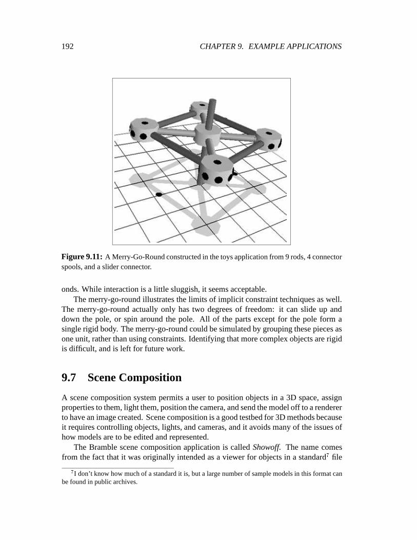
192 CHAPTER 9. EXAMPLE APPLICATIONS
Figure 9.11: A Merry-Go-Round constructed in the toys application from 9rods, 4 connectorspools, and a slider connector.
onds. While interaction is a little sluggish, it seems acceptable.The merry-go-round illustrates the limits of implicit constraint techniques as well.
The merry-go-round actually only has two degrees of freedom: it can slide up anddown the pole, or spin around the pole. All of the parts exceptfor the pole form asingle rigid body. The merry-go-round could be simulated bygrouping these pieces asone unit, rather than using constraints. Identifying that more complex objects are rigidis difficult, and is left for future work.
9.7 Scene Composition
A scene composition system permits a user to position objects in a 3D space, assignproperties to them, light them, position the camera, and send the model off to a rendererto have an image created. Scene composition is a good testbedfor 3D methods becauseit requires controlling objects, lights, and cameras, and it avoids many of the issues ofhow models are to be edited and represented.
The Bramble scene composition application is calledShowoff.The name comesfrom the fact that it was originally intended as a viewer for objects in a standard7 file
7I don’t know how much of a standard it is, but a large number of sample models in this format canbe found in public archives.

9.7. SCENE COMPOSITION 193
format called OFF. Showoff is not an application in the traditional sense, but rather, itis a framework for building demonstrations of interaction techniques for scene compo-sition problems. Unlike other applications, Showoff does not create windows or fill thescene with graphical objects. Instead, it defines Whisper functions that make it easy forscripts to do these tasks. For instance, it defines a functionthat automatically createsa framed view, complete with a standard camera and buttons along the side to set var-ious viewing modes. Showoff creates commands for finding andmanipulating objectaspects.
Showoff’s main role is for testing and demonstrating attributes and interaction tech-niques for 3D applications. The typical showoff script creates some objects to providea sample scene, sets up some initial controls and constraints, and begins the interactiveloop. Showoff binds keys and menus to commands for many standard interaction tech-niques. For example, mouse buttons can be used to grab a pointwith the mousepole orthrough-the-lens with either soft or hard constraints.
Showoff has been the primary vehicle for experimentation with controls for posi-tioning objects, lights and cameras. A wide variety of controls are provided for theuser, or the script, to mix and match. Figures 8.3, 8.5, 8.10,and 8.8 are all scenes fromShowoff demonstrations.
Showoff provides few features aside from those used to manipulate scene objects.For example, the interface does not help the user create objects, they must be created bywriting Whisper code. However, Showoff does contain an extensive set of commandsthat allow the differential approach to be applied to the problem of scene compositiondirectly. Showoff presents the user with a large range of controls, including most ofthe attributes of Section 8.1, that can be applied as needed.Controls are combined bylocking: any control can have its value nailed in place. The idea is that the user willemploy a set of constraints and controls that conveniently described the image to becreated.
Showoff does not address the difficult problem of determining how to present a widerange of controls to a user. A sufficient number of controls are available in Showoffthat accessing them is a problem. Showoff uses a haphazard combination of menus,keys, and buttons to specify operations. The interface is “designed” to maximize thenumber of controls made available to the user, even at the expense of usability.

194 CHAPTER 9. EXAMPLE APPLICATIONS

Chapter 10
There are two times in his life when a man should notspeculate: when he can afford to, and when he cannot.
— Mark Twain
Evaluation and Future Work
In this thesis, I have presented a differential approach to graphical interaction: a sys-tematic approach to realizing graphical manipulation based on numerical constrainttechniques. In this concluding chapter, I will review the contributions of the thesis,evaluate the work in light of the goals, and suggest some directions for future work.
10.1 Contributions
The central contribution of this thesis is to develop and demonstrate an approach forrealizing graphical manipulation based on numerical constraint techniques. The thesisextends previous work in interactive physical simulation into a general approach forgraphical manipulation with contributions in the following general areas:
� abstractions for graphical interaction;
� numerical constraint techniques for graphical applications;
� implementation techniques for numerical computations;
� software architecture for graphical applications;
� interaction techniques;
� graphical applications.
This section reviews the specific contributions of the thesis.I feel that the biggest contribution of the thesis is not any of the individual pieces, but
rather, how all the pieces can be fit together. To create the differential approach requiresa new set of abstractions that define graphical manipulationas constrained optimization,mathematical methods to solve the constraint problems, implementation methods toaddress the practical issues in employing mathematics in interactive systems, and asoftware architecture to enable applying the approach and building applications. Onlywith all of these pieces can novel interaction techniques and applications be created.Here we discuss the specific contributions in more detail.
195

196 CHAPTER 10. EVALUATION AND FUTURE WORK
10.1.1 New Abstractions for Graphical Manipulation
At the core of the differential approach is a view of graphical manipulation as a con-straint solving problem. Interaction techniques are created from connectors, controllers,and the passage of time.
� Equation solving as a general abstraction of graphical manipulation: the dif-ferential approach treats graphical manipulation as an equation solving problem.Previous work has used numerical equation solving and optimization for inter-active control in specific cases and non-interactive control of geometric objectswith general constraints. However, no one has previously explored numericaloptimization methods as a general mechanism for implementing graphical ma-nipulation.
� Connectors and controllers as basic abstractions for building graphical ma-nipulation techniques: the concise set of abstractions provided by the differen-tial approach are quite different than any previous ones. They can be combinedand composed. One key feature of the interactive controls inthe differential ap-proach is that they are combinable: if we can control A, and wecan control B,then we can control A and B simultaneously.
� Application of numerical constraint solving to interaction technique design:interaction techniques are described by sets of controls and constraints that areenabled and disabled at appropriate times. This leads to concise, directly ex-ecutable descriptions of classes of interaction techniques that have been diffi-cult to specify, such as 3D widgets. Freeman-Benson’s Kaleidoscope ’91 system[FBB92] defined interaction techniques and widgets by dynamically switchingsets of constraints and previous work such as Olsen and Allan[OA90] and theGarnet system [MGD+90] have used constraints to describe the behavior of 2Dwidgets. However, by employing numerical techniques, the differential approachpermits a richer set of constraints including inequalities, to be used to specifywidgets in a way that automatically defines its inverse mapping from input tovariable.
� A method for describing interactions independent of the underlying repre-sentations of the graphical objects:interaction techniques are defined in termsof the objects’ attributes. The equation solving mechanisms map changes to theunderlying parameters.
10.1.2 Numerical constraint methods for graphical applications
The use of numerical constraint techniques for graphical applications began with therelaxation techniques used in Sketchpad[Sut63]. More recently, there has been inter-est in the related methods of non-linear constrained optimization, non-linear equation

10.1. CONTRIBUTIONS 197
solving, and physical simulation. The problem solved by thedifferential optimiza-tion is very similar to the problems solved at the core of these methods. The solutiontechniques discussed in this thesis are variants of standard mathematical techniques forsolving relatively standard problems.
The methods used in the differential approach are the methods used for interactivesimulation. The techniques described in [WGW90] have been extended by applyingsome standard mathematical techniques, such as damping (Section 3.2.1). This thesisbrings these methods to the domain of user interface design and construction. Previouswork attempting to apply numerical controls to the design ofinteractive systems hasbeen plagued by starting from inferior mathematical foundations.
� Demonstrations of the practicality and utility of the differ ential approach:the running systems show that general controls for graphical manipulation canbe implemented, and perform acceptably on existing computers.
� Application of damping to constraints in interactive graphics: the differen-tial approach uses damping methods (Section 3.2.1) to provide stability in ill-conditioned cases, and to handle over-determined cases. These singular caseshave plagued many previous systems. Damping methods are well known inthe optimization community, and have been applied to similar domains, suchas animation and robotics. This thesis introduces the use ofselective damping toachieve constraint-hierarchies.
10.1.3 Implementation Techniques for Numerical Computations inInteractive Systems
Another contribution of this thesis is the methodology for solving the numerical com-putations required for constraint approaches in a manner that addresses the issues ofinteractive systems. The work of this thesis refines the earlier work on interactive phys-ical simulation.
� Snap-Together Mathematics:the work described in Chapter 5 is a descendantof earlier tools for dynamic function composition and derivative evaluation. Thebasic ideas behind Snap-Together Mathematics, such as explicit representation ofexpression graphs, compile time definition of new function blocks using a sym-bolic math system, and sparse-vector-passing, forward mode, automatic differ-entiation remain from its earliest ancestor described in [WK88]. Several details,such as how variables are handled, have been refined with evolution. The currentimplementation is the first to be incorporated into a higher level toolkit, and thefirst to exploit the generality in a range of applications. Snap-Together Mathe-matics and its ancestors are very different from most other automatic differen-tiation tools which focus on large, dense problems statically defined at compiletime[BGK93].

198 CHAPTER 10. EVALUATION AND FUTURE WORK
� An encapsulation of numerical constraints:Snap-Together Math’s simple pro-tocol for connector outputs, combined with its objects for constraints and con-straint engines, provide facilities for defining (and solving) constraints on equa-tions without seeing the underlying mathematics. TheConstEngine class hasbeen used with other solvers, such as Newton-Raphson.
� Generalization of performance methods for numerical constraints in inter-active systems:the performance methods of Chapter 4 have they been used inprevious systems. However, the work of this thesis shows howall can be inte-grated in a general fashion. In particular, the scatter–gather mechanism of Snap-Together Mathematics, coupled with variable selection mechanisms and variablemerging mechanisms provides a generalized substrate for speeding numericalcomputations through switching between explicit and implicit constraints andpartitioning.
10.1.4 Software Architecture for Graphical Applications
This thesis described Bramble, an object-oriented toolkitbased on the differential ap-proach. The main contributions of Bramble are:
� A graphics toolkit encapsulating numerical constraint methods: Brambleencapsulates the differential approach in a manner that provides services insidethe abstractions of an object-oriented graphics toolkit. In fact, Bramble per-mits building graphical applications with constraints without referring to any-thing other than the typical abstractions of an object-oriented graphics toolkit.This is important because designers of interactive systemsseem to be resistantto learning about mathematical techniques.
� Demonstrations of the impact of the differential approach on application ar-chitecture: by providing generalized methods for mapping between controls andparameters and by permitting connectors to be attached without knowing whatis behind the connector, the differential approach fostersmodularity, parameterindependence and common code. This is seen in Bramble since objects, con-straints, and interaction techniques can all be created independently and hookedtogether as needed.
� A graphics toolkit that facilitates providing general constraints and controlsto users: Bramble aids applications in providing constraints and multiple con-trols to the user. Previous toolkits have used constraints as an internal abstractionto aid the programmer, but Bramble’s focus is providing themas a user level ser-vice.

10.1. CONTRIBUTIONS 199
� Use of a time continuous input model in a graphics toolkit: the differentialapproach provides a continuous model of time, with events integrated as instan-taneous impulses. For a graphics toolkit, the model allows simultaneous asyn-chronous actions to be handled without explicitly programming them into eachevent handler or providing for multi-threaded flow of control. A fundamental dif-ference between this strategy and standard approaches is that handlers for con-tinuous actions such as dragging are instantaneous event handlers, they do notremain active over the duration of the operation, for example from mouse downto mouse up.
� An object oriented graphics toolkit specifically designed for prototyping of2D and 3D applications and techniques.Much of the rationale for Bramble isbased on the intention of its use for prototyping a variety ofinteractive graph-ical applications. This led to exploring a different point in the design space ofinterface toolkits. Because the art of toolkit design, especially for 3D, is stillevolving, explorations of new points in the design space arestill useful. Inter-estingly, other 3D-only graphics toolkits with emphasis onrapid prototyping,including UGA [CSH+92], MR [SLGS92], Alice [PT94], and VB2 [GBT93],have independently made some similar choices.
10.1.5 New Interaction Techniques
In order to demonstrate the differential approach, this thesis presents a variety of in-teraction techniques, many of which are novel enough to be considered contributions.Without user testing, it is in many cases difficult to claim that these are clear improve-ments over previous methods. In fact, some of the new techniques may be unusablein practice. However, I think that a few are interesting. Also, I think the differentialapproach will lead to many new good interaction techniques because it permits provid-ing the advantages of direct manipulation, such as continuous feedback and kinestheticcoupling, to a broader class of interactions and objects.
� Through-the-lens camera controls:these techniques permit manipulating vir-tual cameras and graphical objects by controlling and constraining points in theimage seen through the cameras lens. The methods can be used to address im-portant problems in computer graphics, such as the image registration problemof Section 8.2.4.
� Generalized snapping:(Section 8.4.1) the snapping controller permits any at-tribute of a graphical object to be snapped to precise values, even if they are awayfrom the cursor.
� Interactive manipulation of color to control object and light geometry: theuse of the lighting model equation as a control permits manipulating light color,

200 CHAPTER 10. EVALUATION AND FUTURE WORK
light position, surface colors, and surface geometry. Previous systems containspecial case code for such techniques for controlling lightcolors and surfaceproperties.
� Generalization of interactive control of reflections: the methods of Section8.1.6 permit constraining and directly controlling the positions of reflections onplanar and curved mirrors. The only previous technique was restricted to manip-ulating object translations by dragging reflections in planar surface[HZR+92].The reflection controls also provide a generalization of thespecular highlightpositioning methods of Poulin and Fournier[PF92], permitting the positions ofspecular highlights to be constraints, and to control the geometry of the objectsin addition to that of the light source.
� Generalization of the use of shadows as controls:Section 8.1.6 introducedtechniques to constrain and control object geometry and light positions by con-trols placed on shadows on both plane surfaces and other objects. This permitsa generalization of the Brown interactive shadow widgets[HZR+92] and Poulinand Fournier’s positioning of lights by moving shadows[PF92].
� Scene composition by mixing and matching controls:(Section 9.7) whilesome of the scene composition controls have appeared as special purpose hard-coded controls, no previous system has allowed interactively specifying and com-bining constraints and controls for camera positioning, lighting specification, andobject manipulation.
� Augmented snap-dragging:Briar (Section 9.1) introduces an extension of pre-vious constraint inferencing techniques that permits automatic generation of avariety of geometric constraints from drawing operations.Conversely, the draw-ing methods of snap-dragging [BS86, Bie89], are augmented to also specify con-straints.
� Techniques for displaying and editing constraints in a constraint-based draw-ing program: Briar (Section 9.1) introduces a number of novel methods fordisplaying and editing constraints in a drawing program. Itintroduces a visualsyntax for displaying constraints “in-place” in a manner that parallels their defi-nitions, and two methods for deleting constraints.
10.1.6 Graphical Applications
The primary contribution of the applications described in this thesis is to demonstratethe viability of the differential approach, and the flexibility of the implementation. Al-most all of the applications are re-implementations of other applications using the tech-niques of the differential approach.

10.2. EVALUATION 201
� An interactive Tinkertoys application: the Tinkertoys application permits in-teractive assembly and experimentation with 3D objects mimicking the real toys,including their kinematic behavior. Previous systems, such as those by Surles[Sur92c] and Schroeder [SZ90], either do not provide for interactive editing ofthe objects or they do not permit the simulation of the kinematic behavior.
� User defined shapes with constrained behaviors:thedefine-shape facil-ity in Bramble permits end users to dynamically define new types of shapes in a2D drawing program, and have these objects be manipulated without specifyingthe inverse transformations. Some systems, like the commercial drawing pack-age Visio [Sha93], permit users to define shapes with equations, but do not allowthese shapes to be manipulated except by directly controlling the parameters, anddo not allow the use of constraints in defining shapes.
10.2 Evaluation
This thesis takes a step towards the goal of improving the quality and range of inter-active graphical applications, by providing a substrate onwhich interaction techniquesand applications can be built.
10.2.1 Basic Questions
The central premise of this thesis is that the differential approach can provide an im-plementation of direct manipulation that uses numerical constraint methods to mapcontrols to object parameters in a systematic fashion, and that several issues in directmanipulation interfaces can be addressed by such an approach.
The differential approach does provide a way to implement direct manipulation,as shown by the recreations of other direct manipulation interfaces using the approach.The approach uses a single numerical solver to map a wide variety of controls to a widevariety of objects. This thesis presents a sufficient set of mathematical and implemen-tation techniques to realize the approach, as illustrated by the prototype implementa-tions. These prototypes show that the methods have acceptable performance on currentcomputers. Traditional direct manipulation operations take only a few milliseconds ofcomputation per frame, and reasonable sized constraint problems can be handled atinteractive rates (performance of the prototypes is discussed in Appendix B).
The examples show that the differential approach is interesting. The approach cancreate desired interfaces, often in ways that are more flexible and general than tradi-tional implementations. The approach also permits the creation of new interfaces thatwould be difficult or impossible to create with conventionalmeans. For example, de-spite the utility of methods like the image alignment technique of Section 8.2.4, usersare typically provided with controls less suited for the task because of the difficulty

202 CHAPTER 10. EVALUATION AND FUTURE WORK
in deriving the mapping from the controls to the underlying parameters. While thespecial-case example of the table controls for image alignment might have been derivedby hand, the more general approach of mixing and matching though-the-lens controlscould not have been. In fact, without the view that anything that can be computed canbe a control provided by the differential approach, techniques like through-the-lenscamera control might never have been dreamed of.
10.2.2 Evaluating Abstractions
The abstractions for creating interfaces provided by the differential approach havemany desirable properties:
� the set of abstractions is small;
� they provide concise definitions for many interaction techniques;
� they describe manipulation without reference to the underlying parameterization;
� they can be combined and composed;
� they allow modularity by permitting objects, constraints,and controls to be de-fined independently and hooked together as needed;
� they map directly to the data structures in the implementation;
� they foster a view of manipulation that helps lead to novel interaction techniques.
The abstractions have their problems and limitations, which will be surveyed in Section10.2.7.
10.2.3 Evaluating Differential Techniques
Mathematical and numerical methods are crucial to the differential approach. Withoutmethods that solve the constrained optimization problems in a manner that meets thedemands of interaction, an approach to graphical manipulation based on constrainedoptimization is impossible. The prototypes show that methods exist that permit thedifferential approach to be realized. Section 1.1.4 introduced a number of goals for themethods. Here, we review them:
1. Flexibility in the types of controls: the methods permit the use of arbitrarydifferentiable functions over continuous valued variables as controls. The rangeof controls discussed in Section 8.1 illustrates this flexibility. In practice, therange of controls is limited by numerical considerations.

10.2. EVALUATION 203
2. Freedom to combine controls arbitrarily and dynamically: the solver handlesarbitrary numbers of simultaneous controls, without concern for what they are.This allows controls to be combined arbitrarily. In contrast to many other meth-ods, there are no restrictions on acyclic dependencies or existence of a proceduralsolving plan. Adding a new control requires only passing more equations to thesolver. The flexibility in combining controls is an essential part of the approach.
3. Keep the good properties of direct manipulation: the differential approachallows the creation of interfaces with the good features of direct manipulationsuch as rapid feedback, continuous motion, and kinestheticcorrespondence.
4. Choose the “best” solution in under-determined cases, and find a “reason-able” answer if there is no exact solution: in underdetermined cases, the opti-mization objective defines the “best” solution. The dampingmethods of Section3.2.1 handle overdetermined situations, providing robustness in ill-conditionedcases, allowing for redundant controls, and blending conflicting controls.
5. Provide freedom in picking representations independent from user concerns:because controls are defined in terms of object attributes, rather than their inter-nal parameters, programmers have the freedom to select representations basedon other concerns.
6. Allow a standard procedure for defining new controls that minimizes theamount of difficult mathematical work in defining a new type of control:to serve as a control, a function must compute its value and the derivatives ofits value with respect to its variables. The derivatives canbe computed usingautomatic methods given the attribute’s function, which must be known anyway.
7. Allow a solving mechanism that is general purpose and encapsulatable: thesolving mechanism for the differential approach works on a set of functions, vari-ables, and controllers that specify desired derivative values. Therefore it appliesto problems of controlling differentiable functions of continuous variables. Snap-Together Mathematics encapsulates the solving mechanism,providing the solveras a black box object whose details are hidden from the programmer using thetoolkit. Bramble demonstrates this: it does not even provide the application pro-grammer with the ability to look at solver internal data structures.
8. Work in a variety of domains: the approach is not specific to any particulardomain. A wide range of graphical applications can make use of it.
9. Be fast and scale well:as detailed in Appendix B, the prototype implementa-tions show that the methods can provide sufficient performance on the presentgeneration of computers. TheO(n
2
) computational complexity is a potential

204 CHAPTER 10. EVALUATION AND FUTURE WORK
problem. At the present time, models with 50-100 simultaneous constraints canbe handled.
10. Not require sophisticated numerical techniques:the methods only require nu-merical algorithms to solve easy forms of standard numerical problems. Stan-dard algorithms from textbooks were sufficient for the prototype implementa-tions. Fancier numerical algorithms, such as an efficient sparse singular-valuedecomposition solver or a better ODE solver, may improve performance.
10.2.4 Evaluating the Interaction Techniques
This thesis provides tools for creating graphical interaction techniques. The tools donot necessarily lead to better interfaces, in fact, the tools give interface designers newways to create bad interfaces, for example by applying controls “behind the users back.”However, the differential approach would not be interesting if it only permits the cre-ation of bad interfaces.
The differential approach can be used to create good interaction techniques. Al-though no formal evaluations were done, the techniques demonstrated with the ap-proach include several time-tested standard interfaces, as well as some interfaces thatapply direct manipulation to problems that it previously could not be applied to.
Using the differential approach to recreate existing interaction techniques is notnecessarily overkill: the methods provide a new way to definethese techniques in arepresentation-independent fashion and permit the techniques to be coupled with otherconstraints. The approach can also make implementation easier as it does not requirethe programmer to derive the mappings from controls to parameters.
A more exciting use of the differential approach than recreating existing interfacesis creating of new interaction techniques and constraint-based interfaces. I believe thatthe differential approach can often lead to interesting newtechniques for graphicalmanipulation tasks. The approach has the benefits that:
1. it preserves the continuous motion animation and rapid feedback properties gen-erally desired in graphical interfaces;
2. it permits the creation of controls directly relevant to the users task;
3. it speeds experimentation with new control types as the mathematics does notneed to be derived for each new one;
4. it speeds experimentation by allowing controls to be combined.
The image registration interface of Section 8.2.4 exemplifies all these points. It pro-vides an interface to an important problem, for which conventional interactive controlsare not convenient. The through-the-lens controls are directly relevant to the task, as

10.2. EVALUATION 205
they permit directly specifying where in the image a point inthe 3D scene should ap-pear. The creation of the through-the-lens control required knowing only functionsthat were needed for drawing1. Initial experimentation with the alignment techniquemerely required applying 4 through-the-lens controls. Since through-the-lens controlswere already available in the toolkit, the only new code required to create the interactiontechnique was code to place the video image as the screen background.
The image alignment technique would have been very difficultto create with tra-ditional approaches for implementing direct manipulation. Deriving the mapping fromcontrols to camera parameters is extremely difficult, as canbe seen in the photogram-metry literature mentioned in Section 2.4.2. The more general approach of mixing andmatching controls, used in Showoff (Section 9.7), would be impossible because suchderivations must be done for every new combination of controls.
Unfortunately, the range of interaction techniques that I have developed with thetools of this thesis is not as extensive as I had hoped. Much more of the effort of thethesis research went into tool building. Through-the-lenscontrols were the biggestsuccess. Most other techniques, such as generalized snapping, the scene compositioncontrols such as shadows and reflections, and 3D widgets werenot explored sufficientlywell to make persuasive evaluations of. The success of colorcontrols, something I hadhigh hopes for initially, was thwarted by technical problems. Numerical issues causethe lighting equations not to serve well as controls. Further exploration of these controlsmay find solutions to these difficulties, especially now thatthe solver has dampingcorrectly implemented.
Generalized snapping, described in Section 8.4.1, is another interaction techniquesthat I was unable to explore sufficiently. Some issues are described in Section 10.3.
10.2.5 Evaluating the Architecture and the Prototypes
The prototype implementations described in this thesis consist of a few major parts.Code sizes listed are for C++ source files, with comments, notcounting headers.
� Math and Data Structures Library — (5K lines of C++ in 22 files) My C++math and data structures library includes various basic mathematical elementssuch as matrices, vectors, and ODE solvers as well as more general data structuressuch as lists, queues, and hash tables.
The math library has been used extensively over the past 5 years in a variety ofapplications. Particularly good design features were the object-oriented encap-sulation of sparse matrices and ODE solvers. The code is veryportable, and runson a range of machines from notebook PCs to high performance workstations.
1Arguably, the viewing transformations are in the graphics toolkit, and therefore not known to the ap-plications programmer. However, under this argument, through-the-lens controls are also in the toolkit,so their functions are not known to the programmer.

206 CHAPTER 10. EVALUATION AND FUTURE WORK
It is significant to note that despite the more than 50,000 lines of C++ code in thecomplete system, for reasonable sized problems, the majority of time is spent ina few inner loops of the routines in the library. A fast and robust implementationof basic mathematical data types such as vectors and matrices is crucial to thedifferential approach. Fortunately, such routines are nothard to create and canbe nicely encapsulated in a manner that allows reuse.
� Snap-Together Math Library — (3K lines of C++ in 16 files, several hundredautomatically generated by BlockMaker, 300 lines of Mathematica to implementBlockMaker) The Snap-Together Mathematics library is discussed in Chapter 5.It supports function composition and evaluation, the differential solver, and anumber of predefined function blocks.
Snap-Together Mathematics has proven to work really well. The tool has evolvedsince the earliest versions, but the basic design is the same. Sparse sparse vectorpassing, global time-stamps, and the minimal protocol haveall remained. Thelibrary has been used for a number of applications besides Bramble, includingSpacetime motion control, physical simulation, and statistical data fitting.
The biggest successes of Snap-Together Mathematics are theplaces where it isthe simplest, such as the minimal protocol and the global time-stamp cache val-idation. Better support for features like partitioning andrepresentation switch-ing should be easy to add. One design flaw is that Snap-Together Mathematicsobjects, in particular function blocks, are a bit “heavy.” That is, they can beexpensive to create and destroy.
� Whisper Interpreter — (9K lines of C++ in 18 files, 3K of which were gener-ated semi-automatically by EMACS macros to implement primitives for Snap-Together Mathematics and GL, 800 lines for an interface to animage processinglibrary) The Whisper interpreter is a C++ library for embedding in interactiveapplications. The library contains interfaces for Snap-Together Mathematics,the GL graphics library, and a small image processing library. There are ap-proximately 400 built-in primitives and 20 predefined types, not including whatBramble adds.
Whisper has been a very useful tool for the research describedin this thesis. Ithas been particularly pleasant to program in and to use as a basis for Bramble.Because it was designed for embedding, it provided the rightset of functional-ity to the systems it was put into. It is extremely easy to extend. The simpledynamic object systems is particularly well suited for the kinds of exploratoryprogramming done in an experimental toolkit like Bramble.
� Bramble — (40K lines of C++: including 15K lines of C++ for basic parts in-cluding some automatically generated code, 5K lines C++ forthe 2D library in-cluding automatically generated code for a variety of objects, 7K lines C++ for

10.2. EVALUATION 207
the 3D library, 7K lines of automatically generated function blocks, 700 lines ofWhisper library code) Bramble is the C++ interactive graphics toolkit describedin Chapter 7.
Bramble has been an interesting testbed for the developmentof the differentialapproach. It has facilitated experimentation with the variety of interaction tech-niques and applications discussed in the thesis. I think thedesign of Brambleis quite solid. However, the implementation itself was hastily put together, andshows signs of its unusual evolution, for example before Whisper, other mecha-nisms for many of the object services had to be provided and remnants of thesestill haunt Bramble.
The abstractions of Bramble were sufficient to create a variety of applicationswithout bypassing the approach. This is best illustrated byToys which containsmany features, but is written entirely in Whisper. Bramble ismissing many of thefeatures of standard toolkits, such as text handling. This makes it hard to buildcomplete applications.
� Applications — (230 lines of Whisper forBoxer , 800 lines of Whisper forMechtoy , 500 lines of Whisper forPoly , 500 lines of Whisper forShowOff ,several hundred lines Whisper forShowoff demos, 900 lines of Whisper forTinkertoys ) The complaint with the applications is that there are too few,that they are too small, and not “complete” enough. They do demonstrate thedifferential approach. However, there is much more to a graphical applicationthan manipulating graphical objects. I have been disappointed by my inability tofind a “killer” 3D application.
I believe that the architectural organization of the systemworks out very well. Snap-Together Mathematics provides a good degree of separation between the solver and theclient application. It also allows objects to be defined independently, yet still connectedtogether, by providing a common protocol.
Besides Snap-Together Mathematics, the most significant architectural decision inBramble was the use of Whisper. I believe that this is a good strategy. The dynamicobject system is extremely useful in a graphics toolkit. Thefacility for rapid prototyp-ing is extremely useful in an experimental system. The embedded interpreter approachalso facilitated additions to the toolkit: each new featureor object type did not requireextensive installation into all of the applications. Instead, each new feature simply de-fined new primitive function calls that could be called as needed from applications, oreven interactively from the interpreter prompt. The same functionality might have beenattainable if a development environment such as LISP or Scheme were used, however,such environments did not offer the floating point performance of C++, the ease oftransporting executables, the availability of graphics and numerics packages, nor weregood compilers available at the time that the project was begun.

208 CHAPTER 10. EVALUATION AND FUTURE WORK
As in the process of constructing any system of this size, a lot of design decisionswere made along the way. Some of the best design decisions that I made were (in noparticular order):
� the simple protocol for Snap-Together Mathematics;
� using an embedded interpreter in the toolkit;
� using the Whisper object system for graphical objects;
� half sparse matrices;
� using a conjugate-gradient solver;
� the scatter gather handling of state variables.
Some of the worst design decisions I made were:
� using the simple GL event model of handling events globally,rather than han-dling events on a per-window or per-object basis. Also, GL does not time-stampevents, nor record the mouse state when an event occurs. Thiscauses problemswhen event handling is delayed as the mouse may move between when the eventhappens and when the event is processed;
� having a single world, rather than explicit scene graphs like Inventor [SC92].This makes it impossible to edit multiple documents, and difficult to show dif-ferent data in different views.
� creating my own widget library. Many toolkits containing basic widgets suchas buttons and sliders are available. Using these would havegiven more attrac-tive looking widgets, and probably some richer functionality such as file-selectordialogs.
10.2.6 Experience with the Implementations
Because of the large overhead of making tools available to others, an explicit decisionwas made in the research plan for this thesis not to make the tools available to others.
After many requests, I have made the Snap-Together Mathematics library publiclyavailable by anonymous FTP access. Because I did not offer support or documentation,I suspect that few people have made extensive use of it. A small number have reportedsuccessful experiments built with Snap-Together Mathematics. One CMU undergrad-uate student was able to build a portable 2D version of Point Tinkertoys that ran underthe X window system, without learning anything about the constraint mathematics. I

10.2. EVALUATION 209
also know of at least three re-implementations of Snap-Together Mathematics by re-searchers who had access only to the papers. These researchers were able to build 3Dconstraint demonstrations.
Bramble was not offered to others because of the amount of support it would require.Because of this, I cannot make any claims about how “usable” Bramble is. Personally,I find Bramble a joy to use. Part of this may be attributable to the fact that I designedBramble based on my personal tastes and program developmentstyle. The interpre-tive environment and high level language of Whisper extremely appealing comparedto C++. However, I believe that a good part of Bramble’s attraction is how well theabstractions fit the needs of graphical application development.
Other than myself, the main users of the applications in Chapter 9 have been peo-ple who have “taken over the drivers seat” during demos. Thishas allowed informalassessments of how users react to interaction techniques created with the differentialapproach. Such users are atypical: since they are only playing with the applications fora few minutes, their usage patterns are different than thoseof users’ attempting to solvereal problems. For example, many people permitted to use thesystems immediately totry to torture the solver by making impossible connections to see what happens.
Response to the applications has been very positive. Few complain about the lagbetween the pointer and the object being dragged. In fact, many comment on how theylike the feel of it. Some things, such as dragging the spiral of Section 8.1.1 generallyrequire a little practice before people can achieve the effects that they intend. However,almost everybody has been able to figure it out without instruction. There is little elseto compare these systems to in terms of usage.
I am consistently impressed by how quickly people learn to use the mousepole aftergetting past the initial issue of using multiple buttons on the mouse simultaneously. Ingeneral, people seem to like the Bramble standard 3D interface. Part of this may beattributed to relative novelty of interactive 3D graphics,and to the attention to aestheticdetails such as the use of shadows and the selection of colors.
10.2.7 Limits and Drawbacks
The drawbacks of the differential approach, as seen in this thesis, fall into three cate-gories:
1. fundamental limitations or drawbacks of the approach;
2. limitations and drawbacks of the techniques that should be resolved by futurework;
3. artifacts of the prototype implementations.
The fundamental limitations of the approach are:

210 CHAPTER 10. EVALUATION AND FUTURE WORK
� The differential approach is time continuous.Things do not happen instanta-neously. While this is generally a feature, some times we wantobjects to jumpto their destinations, for example, when a new object is created.
� The differential approach only is applicable to continuously valued parame-ters and attributes. The numerical methods do not apply to discrete data. Somealternate mechanisms, such as propagation constraints, must be used.
� The methods do not scale as well as those for other approaches.Without re-stricting the problems, the complexity bound ofO(n
2
) seems to be unavoidable.
Some major limitations that I think can be addressed in future work are:
� scalability: While O(n
2
) is the limiting factor, methods to reducen and theconstants can allow solving larger problems. Implicit constraint methods canpotentially enhance scalability considerably, as demonstrated in the Tinkertoysapplication. Also, it is unclear how large the number of controls a system musthandle. For predefined objects and interaction techniques,the number of controlswill be a (usually small) fixed number (e.g. it will not grow with problem size).However, with a constraint-based interface, a user may create arbitrary numbersof controls. But, this number may not be unbounded as eventually, the limits ofhow much simultaneous behavior a user can comprehend may be reached.
� precision: Methods for more precisely achieving the user’s goals will facilitatemany applications. Generalized snapping is a first attempt.
� generality: As described in Section 8.1, mathematical considerations cause somefunctions to work better as controls than others. Some formal characterizationfor which controls which and what do not would further simplify the constructionof interfaces.
� real-time: Adding a coupling to real (e.g. wall-clock) time would increase theexpressibility of the abstractions. Interface designers would gain control over thetime constants involved in the approach.
� integration: The differential approach applies only to the continuous motiondragging parts of applications. Therefore, integration with other techniques, suchas propagation constraints, to handle other parts of applications is essential.
� hierarchy: The methods for differential constraints provide only two levels ofconstraint hierarchy. The work of Borning et al.[BFBW92] shows the usefulnessof more levels.
Many of the problems in the prototypes are artifacts of the implementations, ratherthan problems with the approach. They fall into three general categories:

10.3. DIRECTIONS FOR FUTURE WORK 211
� Bad design decisions:Several bad design decisions were listed in Section 10.2.5.
� Artifacts of evolution: The prototypes evolved from earlier versions, so in manyplaces there are leftovers from early versions. Bramble’s property sheets andSnap-Together Mathematics’s confusing mechanisms for soft controls and gen-eralized snapping are two examples.
� Incompleteness:The prototypes were built in time to finish a thesis, so manyfeatures that are not essential to the points of the thesis have been omitted, suchas text-handling in Bramble.
10.3 Directions for Future Work
This section discusses some topics to extend the differential approach, make effectiveuse of it, or repair its deficiencies.
For this thesis, a number of prototype implementations wereconstructed. An en-tire class of future work involves the creation of more “industrial strength” tools andapplications that can be widely distributed. For Snap-Together Mathematics, this maymainly involve completion of some partially implemented features, documentation andsupport. However, for Bramble, it is probably not worthwhile to go through the effortof making a distributable tool since too many design decisions were made with a “getit done for the thesis” attitude. This section focusses on future work on the differentialapproach more generally, rather than on the specific artifacts of the toolkit.
10.3.1 General Issues
The differential approach’s model of time does not correspond with real time. Thislimits what can be expressed with the approach. For example,it makes it impossible tospecify desired rates in a meaningful way. Some mechanism for correlating simulationtime and real time would be a useful addition to the approach.However, it would re-quire tackling a number of difficult technical issues in synchronization, especially withthe variability of the solving methods. This issue will alsobe increasingly importantin future multi-media applications. Faster processors might help with synchronizationissues since programs will have the possibility of finishingtheir work quickly and thenwaiting for synchronization. However, such “busy waiting,” is not the most effectiveuse of processor cycles, and fails to handle cases where the fast processor’s performanceis needed to handle larger problems.
Future high-performance computers will make the lack of real-time coupling diffi-cult because things may happen too fast. It will be importantto provide the interfacedesigner with some control over the time constants of the interactions.

212 CHAPTER 10. EVALUATION AND FUTURE WORK
The approach lacks a good characterization for what makes a function work wellas a control. The rules of thumb from Section 8.1 need to be formalized. If the char-acterization could be sufficiently codified it would allow aneven more automated toolfor creating new controls to be created.
Precision in manipulation is another issue for the differential approach. Even forSnap andClick controllers (Section 6.4), the exactness of solving is limited be-cause controllers only get to specify velocities at sampledincrements. For greater pre-cision, controllers might need to be given some informationabout step size. This isalso important for better tracking of input devices as it would permit better prediction.Enhancing mouse tracking, for example by predictive filtering, is another area for study.
The lag between pointing device and dragged object needs to be better understood.In applications where the lag is detrimental, it might be reduced by techniques suchas predictive tracking. Developing predictive tracking strategies for input devices willbe generally useful, not only for the differential approach, but also for things such asremote collaboration.
10.3.2 Mathematical Techniques
The weakest link in the mathematical techniques is the way that over-constrained sys-tems are handled. Many of the deficiencies of the damping techniques are listed in Sec-tion 3.2.1. An alternate method of dealing with the ill-conditioned or singular matricesmight be found. To date, I have not found any that retain the performance characteris-tics of the methods discussed in this thesis on well-conditioned problems.
A primary drawback of the damping methods as described in this thesis is that theyalso affect constraints that are not ill-conditioned. Thisdrawback can be avoided byusing methods, such as the one presented by Nakamura[Nak91], that adaptively set theamount of damping. These methods are expensive, as they effectively must solve thesystem to determine its condition. Another strategy would perform some potentiallyexpensive computation to determine if there are bad constraints, and applying the damp-ing methods only in these cases. The hope would be that the expensive computationswould not be needed often or could be computed incrementally.
Alternate methods for handling over-constrained matrices, such as singular valuedecomposition, have better numerical properties than damping, but would require workto make them as efficient. Similarly, more reliable methods for handling inequalities,such as those of Baraff [Bar94], could be applied if efficiency concerns were addressed.
Another deficiency of the methods presented in Chapter 3 is that they offer fewopportunities for levels of importance of controls (hierarchies in the terminology ofBorning et al[BFBW92]). Soft controls provide two levels of constraints, but requirebetter methods to give them the degree of control of hard controls. Extending differen-tial techniques to support more levels of hierarchy would beuseful.
The methods of the differential approach are designed to work with the lowest com-

10.3. DIRECTIONS FOR FUTURE WORK 213
mon denominator of general functions, avoiding special cases and anything beyond theminimal information about the functions. Each of these restrictions could be relaxedto create methods that better handled important special cases. For example, specialmethods for articulated figures exist. Also, more information about functions, such ashigher derivatives and intervals, could also be used.
The techniques provided for handling inequality constraints are really a hack, andwould be improved by using numerical methods better suited for this task. Findingmethods with suitable performance characteristics could be challenging.
10.3.3 Numerical Techniques
As computers become faster, the size of the problems that canbe handled at interactiverates will increase. This means even more of the computationtime will be spent inthe complexity limiting step of solving the linear systems.Selecting appropriate algo-rithms will be increasingly important. Other conjugate-gradient solvers, such as thosefrom [PS82] might apply. In particular, some of these methods may better handle ill-conditioned or singular matrices, allowing less use of damping techniques. Dynamicselection among multiple solvers, as done in Converge[Sis90], may also provide betterperformance, particularly when the problem can be partitioned.
The best weapon against the computational complexity of solving the linear systemswill be to reduce their size while giving the user the illusion that the entire problem isbeing solved. There are many possibilities for new implicitconstraint mechanisms.For example, representations of objects could be dynamically switched to maximizethe number of constraints that are represented cheaply. Algorithms similar to multiple-output multi-way local propagation solvers, like [San94],could implicitly solve asmany constraints as possible. Techniques that divide the problem based on numeri-cal results are possible. For example, Sistare[Sis90] partitions constraints empirically.The solver attempts to solve the constraints on a small subset of the objects. If theseobjects do not have sufficient degrees of freedom, more objects are added to the subset.
Better methods for solving the ODEs would enhance the stability of the constraintsand permit a wider class of controls. Making use of knowledgeabout the expectedbehavior of the objects should provide information that canbe used to adapt the stepsize of the solver. Finding ways of making adaptive step sizes unobtrusive to the usermight be required to make them acceptable.
The simple caching mechanisms of Snap-Together Mathematics are reasonable forthe experiments conducted so far with the differential approach. Cache analysis showsvarying performance of the global cache validation scheme.A better caching scheme,perhaps based on incremental attribute evaluation[Hud91], might be more efficient.However, as problem sizes grow, the cost of the Snap-Together Mathematics compu-tations will become smaller relative to that of solving the linear system. Therefore,extensive optimizations are unwarranted. Better support for switching representations

214 CHAPTER 10. EVALUATION AND FUTURE WORK
would be another improvement in the Snap-Together Mathematics implementation.
10.3.4 Interface Toolkits
The differential approach addresses only a part of the problem addressed by moderninterface toolkits. If the differential approach is to be used in a complete toolkit, it mustbe made to integrate cleanly with existing approaches. Employing propagation solversfor discrete data inside the differential approach seems toprimarily be an engineeringproblem. However, incorporating the differential approach, with its different model oftime, into a conventional event-driven toolkit poses difficult questions such as how tointegrate discrete state changes into the continuous flow oftime.
The ways that the Whisper interpreter supports Bramble bringinteresting questionsas to the architecture of graphics toolkits. Fast turnaround is only one of the reasonsfor the widespread acceptance embedded interpreters in graphics toolkits. However,much of the utility of the Whisper/Bramble connection is thatmany of the services thatBramble must provide, such as object management and on-the-fly definition of behav-iors are similar to those provided by the run-time support for a modern programminglanguage. An interesting strategy might be to design run-time support specifically forinteractive graphical applications.
10.3.5 Interaction Techniques and Applications
While the differential approach has many flaws that may be addressed with future re-search, the techniques and tools are evolved enough that they can be used to createnovel interaction techniques and applications. The invention of new graphical tech-niques will be the real payoff of the approach. Developing new interaction techniquesmay require finding new attributes of objects to constrain and control, new combina-tions of these controls, and new ways to present the controlsand constraints to users.
Generalized snapping is a feature of the differential approach that has not beensufficiently explored. There are many issues in making it into a successful interactiontechnique, such as how to provide adequate feedback to the user and how to determinethe many parameters. However, I think it is still a promisingtechnique.
The availability of a variety of controls and the ability to combine these controls asconstraints opens up a new domain of questions about how to select, specify, display,and edit the controls and constraints. Some tasks, like scene composition, seem particu-larly appropriate for interfaces that give palettes of controls to users. I think the strategyof manipulation from structure is a promising way to help make these tasks easier bybuilding more constraints into the system before the user has to specify anything.
Good controls might also serve to facilitate manipulation when the “user” is somecomputational mechanism automatically controlling the graphical objects. For exam-ple, an automatic picture composition system like those described by Feiner[Fei93]
10.4. FINAL REMARKS 215
might be easier to develop in terms of controls like “point the light at this object” ratherthan directly altering the underlying parameters of the objects.
The ability to handle controls asynchronously may help explore multi-input deviceinteraction techniques. In general, the approach may serveto help incorporate newinput mechanisms as it decouples the input device from the objects being controlled.
There are many questions which must be addressed before constraint-based inter-faces for drawing and modelling can be successful. Constraints must be made easyto display, debug, understand, and edit. While restricted problems, such as permittingusers to define the behaviors of individual objects, simplify these issues, they do notremove them.
The techniques for specifying, displaying, and editing constraints introduced inBriar also deserve to be examined in more detail. Future workmust address issues inextending the techniques to larger classes of constraints,scaling them to larger models,and applying them in 3D.
10.3.6 Usability Evaluation
This thesis provides little in the way of formal evaluation of the differential approach.Because the new interaction techniques were meant only as examples of the differentialapproach, not as wide-ranging solutions to interface problems, it was not appropriateto study the usability of these techniques. However, because some show promise asinteraction techniques, more formal evaluation may be useful.
Much of the lag between pointing device and target object in the differential ap-proach can be reduced with better tracking. However, many users report enjoying this“spring” behavior. A study to evaluate the usability of the spring dragging might be in-teresting. Similarly, the usability of constraint-based graphics has never been formallystudied. Such a study might determine people’s abilities touse multiple simultaneouscontrols, or help understand how complicated a constrainedmodel might be created bya user before comprehensibility is sacrificed.
10.4 Final Remarks
This thesis has provided an approach to implementing directgraphical manipulationthat uses the numerical and graphical performance of modernprocessors. The approachviews manipulation as an equation solving or constrained optimization problem, allow-ing interactions to be defined in terms of objects’ attributes, rather than their represen-tations. To implement the approach, mathematical techniques for solving the optimiza-tion problems had to be selected and implemented in a way thataddresses the issues ofinteractive systems. This implementation permitted encapsulating the mathematics ina manner that allowed the construction of a graphics toolkitthat hid the mathematics of

216 CHAPTER 10. EVALUATION AND FUTURE WORK
the approach from the applications programmer. With the approach and the prototypeimplementations, a number of interaction techniques and applications were created.
Direct graphical manipulation has been widely successful,and future systems of-fer new possibilities and issues for these interfaces. As decreasing cost makes highperformance computers more widely available, graphics tools will have a wider poten-tial audience. Many of these users will require more fluent and transparent interfacesfor types of tools now only used by experts. New classes of applications, such as vir-tual reality, offer whole new classes of issues. New users and new applications willchallenge interface designers. The ad-hoc methods traditionally used to devise manip-ulation techniques will hinder the development of new interfaces. This thesis has offersan alternative that can provide a substrate for future direct manipulation interfaces.

Appendix A
The world is your exercise book, the pages on which youdo your sums. It is not reality, although you can expressreality there if you wish.You are also free to write nonsense, or lies, or to tear thepages.
— Richard BachIllusions,p. 127
The Whisper Programming Language
An important tool in the development of the differential approach has been a simpleinterpreter for a language calledWhisper.Whisper serves four main purposes in thiswork:
1. An embedded interpreter is important for interactive systems to realize featuressuch as saving and loading of models and configuration files.
2. The language runtime provides useful tools for system construction, such as adynamic object system and dynamic function definition.
3. The language provides a convenient notation for describing interaction tech-niques in this thesis.
4. The interpreter permitted avoiding many of the problems with the programmingenvironment available to develop this work, such as slow turnaround and baddebuggers.
Whisper is not directly connected to the differential approach. However, it is dis-cussed here for several reasons. Foremost, the language is discussed enough so that areader can understand the examples written in Whisper in various sections of the thesis.
The Whisper interpreter is specifically designed for being embedded into applica-tions. The primary design goal were simplicity and extensibility, even at the expense ofperformance. Although performance of the interpreter is poor, the ease of extensibilityallows adding speed critical code as new primitives writtenin the host language, C++.New data types can also be added easily to the interpreter. Once the core interpretivelanguage was built, extensions were created to provide access to the Iris GL graphicslibrary, Snap-Together Mathematics, an image processing library (that is not used inthis thesis), and Bramble.
217

218 APPENDIX A. THE WHISPER PROGRAMMING LANGUAGE
A.1 Whisper Basics
Whisper is a lexically scoped variant of LISP, like scheme. Whisper is very similar toother languages in this family. A basic introduction to programming in such a languageis provided by Friedman and Felleisen [FF87]. Rather than providing yet another tuto-rial for such languages, we instead look at the differences between Whisper and morecommon dialects that are relevant to the code examples in thethesis.
Like other LISP dialects, Whisper has dynamic types. All dataare tagged with theirtype, and the types can be determined for any object. Whisper’s type system is extensi-ble at compile time only. The basic set of types provided by Whisper includes integers,floating point numbers, strings, pairs, points (3 floating point numbers), closures, built-in primitive functions, clocks (special objects for timing) and environments. Types forbasic Snap-Together Mathematics classes are provided, as well as for Bramble objects.Almost all Bramble objects have the Whisper typeIDObj , but the subtypes can easilybe determined.
Whisper’s special forms for setting variable values are different from most LISPdialects. Whisper provides aset function that sets the value of a variable. If thevariable is defined in the current scope, it is simply reboundto the new value. If thevariable is not defined, it is created as aglobal variable. Thedefun function used todefine a function is simply shorthand forset. Thebind function acts like set, but italways sets a variable in the most local scope.
Whisper is lexically scoped. Variable bindings are determined by the code thatsurrounds them in the program text. For example,
(let ((a 5))(defun f (x) (+ x a)))
defines a function that adds 5 to its argument. Anenvironmentis the object that em-bodies a scope, that is, it is a pairing of variable names and values. Environments arehierarchical, that is, each environment refers to the environment it was defined in. Un-bound references are deferred up the chain of environments until the global scope isreached.
One important feature of Whisper is that it permits treating environments as firstclass objects. Many dialects of Scheme, such as MIT Scheme [HtM93], do this as well,and the introductory programming text by Abelson and Sussman [AS85] provides anintroduction to the use of first-class environments. Whisper’s syntax and operations forfirst-class environments is different from Scheme’s.
Theenvironment special function returns a reference to the current environmentthat can be passed around as any other data element. For example,

A.1. WHISPER BASICS 219
(set e (let ((a 5)(b 6))
(environment)))
sets the variablee to an environment that bindsa andb. Various operations can beperformed on environments, including adding additional bindings, inquiring as to theircontents, combining two environments, and printing the contents of an environment.
The two most important operations that can be performed are to evaluate an expres-sion within an environment, and to bind a value in an environment. To add a bindingto an environment, a special version of thebind primitive function is used that takesan extra argument for environment, for example,
(bind-in e c 10)
which would add the bindingc = 10 to the environment defined in the previous exam-ple. A similar version ofeval is provided,
(eval-in e (+ a b))
which for the example would return 11. Whisper provides the syntax
( env expr
1
expr
2
: : : expr
n
)
to evaluate expressionsexpr1
throughexprn
in succession inside of the scope of en-vironmentenv: The value of the evaluation of the last expression is returned. Thisconstruction violates lexical scoping, for example,
(let ((a 1)(b 2))
(e (+ a b)))
with e defined as in the above example evaluates to 11, not 3. This cancause an im-portant distinction between the use ofbind andbind-in . For example,
(let ((a 10))(bind-in e f a)(e (bind g a))
creates bindings forf andg inside ofe, however,f will be bound to 10, whileg willbe bound to 5, because its binding statement was evaluated inside ofe.
First class environments function as Whisper’s object system. Fields and methodsare stored as bindings in the environment. The object creator makes an environmentand binds variables to their initial configurations. While there is no explicit mechanism

220 APPENDIX A. THE WHISPER PROGRAMMING LANGUAGE
to provide inheritance or delegation, such functionality can be provided in the creatorfunctions.
A BrambleIDObj is not an environment, however each object carries an environ-ment around. Theget-env function returns the environment carried by anIDObj .Whisper syntax permits using the evaluation notation for Bramble objects as environ-ments, so
( IDObj expr)
is a shorthand notation for
((get-env IDObj) expr).
A.2 Some Examples
In this section, we take a few examples of code fragments fromWhisper programs toexplain various features of the language, and how they are used with Snap-TogetherMathematics and Bramble.
This first example defines a function that builds the functionblock graph for theline segments shown in Figure 5.1. The line segment is returned as a Whisper object,that is, as an environment. Notice that an environment is made first and then the in-termediate values are defined in a different environment. This way the environmentthat will represent the line segment does not contain the intermediate values, only theconnectors.(defun make-line () (let* ((q (make-stobj 3)) (e (environment))) (let* ((c (cos-block (signal q 2))) (s (sin-block (signal q 2))) (lc (times-block c (signal q 3))) (ls (times-block s (signal q 3)))) (bind-in e left-x (plus-block lc (signal q 0))) (bind-in e left-y (plus-block ls (signal q 1))) (bind-in e right-x (plus-block lc (signal q 0))) (bind-in e right-y (plus-block ls (signal q 1)))) e))
;;state vector w/3 spaces;empty "object" to put things in;make blocks to compute ; intermediate results
;make connectors; put the blocks directly into; the object
Calling this procedure returns an environment that contains 6 bindings: 4 for theconnectors, 1 for the state vector and an extra binding that is a reference to itself. Touse these objects to create the wiring of Figure 5.1, given a function to perform the

A.2. SOME EXAMPLES 221
attach operation which would take 4 connectors as inputs andcreate the function blocktree:
(set rod1 (make-line))(set rod2 (make-line))(set nail (attach (rod1 left-x) (rod1 left-y)
(rod1 right-x) (rod1 right-y)))
Attach would return an object (a Whisper Environment) that contained two connectors.It might be defined as follows:
(defun attach (x1 y1 x2 y2)(let ((c1 (minus-block x1 x2))
(c2 (minus-block y2 y2)))(environment)))
The following code fragment is a more expanded example of constraint inferencingusing Bramble’s snapping than the one given in Section 7.7.3. It is a Bramble eventhandler that is used to draw lines with rubber banding and automatic inference of con-straints.(1) (add-key dev-rightmouse k-none k-down (2) (lambda (v) (3) (let* ((s (snapdp)) (4) (p (if s (where s) (cursor-mapw view))) (5) (l (make-2d-line (p-x p) (p-y p) (6) (p-x p) (p-y p))) (7) (d (pt-eq-2d (l end1) (v mouse-port)))) (8) (if s (pt-eq-2d (l end2) s)) (9) (add-key dev-rightmouse k-any k-up (10) (lambda (v) (11) (let ((s (snapdp))) (12) (delete d) (13) (if s (pt-eq-2d (l end1) s))))))))
; define button down handler ; ; get snap point ; start drag at snap or mouse ; create object at start ; ; connect one end to mouse ; if snap, infer constraint ; define button up handler ; ; get snapped point ; delete drag constraint ; if snap, infer constraint
This fragment is a call toadd-key , the Bramble primitive for defining key han-dling events. The first three arguments specify that this call is to define the right mousebutton press (down) event with no modifier keys. The last argument to the call is aclosure that is to be called with one argument when the event occurs. The argumentspecifies the view that the event occurs in.
Lines 2-12 define the procedure that is called when the right mouse button is pressed.First, a number of local variables are bound to various quantities useful in the operation:s is bound to the current state of the snap-server;p is bound to either the position ofs , if there is a point snapped to, or to the position of the cursor; l is bound to a newly

222 APPENDIX A. THE WHISPER PROGRAMMING LANGUAGE
created line segment, created with both endpoints atp; and a constraint is created con-necting one endpoint ofp to the position of the mouse in the current view and storedin d.
Line 7 performs a constraint inference. If the cursor is snapped to a point whenthe line is created, the end of the line is connected to that point with a point equalityconstraint.
Lines 8-12 redefine the event handler that is called when the right mouse button isreleased. Because of Whisper’s lexical scoping, this code isexecuted in the environ-ment created by the key down handler and has access to those local variables. It firstdeletes the constraint that was connecting the line segmentto the cursor. If the cursorwas snapped to a point when the button release occurs, the line segment is attached tothis point in line 12.
A.2.1 The Define-Shape Syntax
A special facility is provided in Bramble to facilitate the creation of 2D shapes. Theprocess is inspired by the shape spreadsheets in the Visio drawing program [Sha93],but has greater utility because it permits placing constraints inside objects and usingany point as a handle. Thedefine-shape special function takes a description ofa shape and automatically generates two functions: one thatcreates instances of theobject, and another that draws a prototype version of the shape suitable for displayingin an icon. Thedefine-shape primitive is special because it does not evaluate itsarguments in the standard way.
The syntax ofdefine-shape are as follows:
(define-shape name variables defaults lets command
1
command
2
: : :)
where:
name is a string that names the type;
variables is a list of state variable names;
defaults is a list of initial values for each variable;
let is a list of let pairs to define internal variables;
command is a pairing of commands and data.
For example, a simple rectangle can be defined by:

A.2. SOME EXAMPLES 223
(define-shape rectangle (w h) (.5 .25)((w2 (/ w 2))
(h2 (/ h 2))(mw (- 0 w2))(mh (- 0 h2)))
(spath ( (w2 h2) (mw h2) (mw mh) (w2 mh) )))
All shapes are defined in their local coordinates, so the rectangle only has 2 state vari-ables, width and height. Default values for these are provided. The let list defines 4local variables. Thespath command defines a list of vertices that are connected todraw a polygon, with handle points placed at each vertex. Thecommand is equivalentto separate commands to define a drawing function and handle points. Literally, thedefinition used for drawing is also used for manipulation.
Thedefine-shape mechanism makes extensive use of Whisper first-class en-vironments to make the concise specification possible. Eachvariable declaration andlet list clause defines a new symbol in the objects local environment. Each of these isbound to a signal: when thedefine-shape is executed, it is run in a special envi-ronment that shadows all of the basic arithmetic operationswith their Snap-TogetherMathematics block generating counterparts. Because the drawing routines do not exe-cute during thedefine-shape , they can do normal arithmetic.
Other commands permit more general drawing commands, explicit specification ofhandle points, and generation of constraints on the object.The fuel-gauge widget ofpage 162 demonstrates many of the features ofdefine-shape . Here we present amore complete version:

224 APPENDIX A. THE WHISPER PROGRAMMING LANGUAGE
(1) (define-shape gas-gauge (sz theta) (.35 0) (2) ((l (* (one-way sz) .9)) (3) (t (+ .2 (* 2.7 theta))) (4) (x (- 0 (* l (cos t)))) (5) (y (* l (sin t))))
(6) (drawf (prog (color gl-white) (arcf 0 0 sz 0 1800) (7) (color gl-black) (linewidth 3) (8) (arc 0 0 sz 0 1800) (9) (move (- 0 sz) 0) (draw sz 0) (10) (icon-font) (11) (cmov (* l -.9) (* l .2)) (fmprstr 'E) (12) (cmov (* l .8) (* l .2)) (fmprstr 'F) (13) (move 0 0) (draw x y) ))
(14) (> theta 0) (15) (< theta 1) (16) (handle x y))
; draw function; white arc for back; black border; arc border; bottom border; set text font; place labels; for E and F; draw needle;; limit to legal values; ; create handle on needle
; 2 params; local variables; size; angle (in radians); positon of needle
The gas gauge has 2 parameters, one for the size of the gauge, and one for its currentvalue. The let clause of thedefine-shape defines a number of intermediate vari-ables using arithmetic operations. One special operation isone-way that defines thatcontrols on its output should not effect its input. Theone-way function block returnsthe value of its input, but always returns a zero derivative.For the gas gauge, the one-way is used so that dragging the needle of the gas gauge does not change the size of thegauge. Thedrawf command defines a code fragment that is used to draw the gauge.The list of statements are calls to the GL graphics library. The > and< commandsdefine constraints, and thehandle command creates aDistinguishedPointconnector at the specified position on the object, which in the example is the tip of thegauge’s needle.
Theinstall-shape function is defined by certain applications to automaticallyinstall an icon for creating shapes defined withdefine-shape . It simplifies usingdefine-shape in an application. Theinstall-shape function takes the valuesreturned bydefine-shape and creates an icon and the proper handlers for creatingnew instances of the shape.
Appendix B
The real purpose of scientific method is to make sure Na-ture hasn’t misled you into thinking you know somethingyou don’t actually know.If you get careless or go romanticizing scientific informa-tion, Nature will soon make a complete fool out of you.It does it often enough anyway when you don’t give it op-portunities.
— Robert PirsigZen and the Art of Motorcycle Maintenance,p. 94
Performance of the Implementations
This appendix provides some empirical tests measuring the performance of the proto-type implementation. The absolute performance numbers are, in a sense, not importantas the hardware and the implementation are continually changing. These benchmarksare provided to:
� Provide empirical evidence of the scaling properties of thetechniques, as ana-lyzed in Section 4.2.
� Give some idea of the scale of problems solvable with currently (circa 1993)available hardware.
� Provide some intuition for where the performance bottlenecks are.
Understanding the performance of a program running on a modern, high-performanceworkstation is a difficult task. Complicated factors such asmemory hierarchy orga-nization interact in complex ways. For example, different problems may distributethemselves differently along the lines of the data cache. Although we have attemptedto design benchmarks that reduce these types of effects, anynumbers must be viewedwith some caution.
The benchmarks were run on a Silicon Graphics Indigo 2 workstation, except wherenoted. The machine had a 150MHz R4400 processor and 32 megabytes of main mem-ory. All of the problems fit into main memory on the machine, sono paging occurred.The clock accuracy on the workstation is 10 milliseconds. Where greater precision isreported, it was found by averaging over enough trials that the extra digit remains stableas more trials are run. Some of the simpler benchmarks were run on a Silicon GraphicsPersonal Iris 4D/25, with a 20MHz R3000 processor, 16 megabytes of main memory,
225

226 APPENDIX B. PERFORMANCE OF THE IMPLEMENTATIONS
Figure B.1: A sample run of the synthetic benchmark withm = 50 andn = 25: Lines areused to denote pairs of points with a control placed between them. Each step, the controls pushthe points closer to one another.
and small instruction and data caches. Current generation personal computers providesignificantly better performance than this older machine. Where figures are providedfor this machine, they will be explicitly noted.
B.1 A Synthetic Benchmark
In order to evaluate the performance and scalability of the solver, a contrived problemwas developed that can be arbitrarily scaled. The problem isdesigned to mimic real-istic problems in which the constraints may have random structure. An instance of theproblem can be defined for any number of variablesm and constraintsn: The problemplacesm=2 points on the plane and placesn controls, each connecting 2 points. Acontrol computes the distance between the points and has aGoTowards controllerplaced on it.
A synthetic workload generator creates instances of the problem. It randomly dis-tributes the points in a 10x10 square. Pairs of points are selected to have the distancecontrols placed on them. The workload generator insures that there are no duplicatecontrols, but makes no other checks on the distribution of the constraints. An examplerun is shown in Figure B.1.
Generating arbitrarily sized synthetic workloads for the solver that are reliable mea-sures of performance is difficult. The speed of the solver depends almost as much on thestructure of the constraint problem as it does on its size. This can create a bias basedon the density of constraints in variables. For example, consider an example with 2constraints. If there are only 3 variables, no matter how the2 constraints are placed,the constraints will be in a single partition. However, if there are 4 variables, the con-straints might not access any common variables, so the solver will partition the matrix.As the number of variables goes up, the probability of this goes up as well. This canlead to the counterintuitive result that for a fixed number ofconstraints, larger numbersof variables might actually be faster to solve. For randomlygenerated problems of thesame size, there can be substantial differences in solving time based on how “hard” thesystem is to solve: if one set of constraints is more tightly connected than another.

B.1. A SYNTHETIC BENCHMARK 227
0
0.5
1
1.5
2
2.5
3
0 50 100 150 200 250 300 350
tim
e p
er
tria
l (s
eco
nd
s)
number of constraints n
Figure B.2: Results of the synthetic benchmark. The ordinate enumerates the number ofcontrols, the abscissa is the time required to run 5 4th orderRunge-Kutta steps. Error barsrepresent the range of time for each value. The central ticksmark the mean values for thetrials. m = 400 variables were used in all trials.
To run the trials, 5 constraint configurations and 5 initial positions were generatedfor each problem size. This leads to 25 different trials per problem size. Each trialwas run for 5 Runge-Kutta 4 steps (that is, the differential optimization was solved 20times). Each trial was duplicated a small number of times.
Graphing the results of running the trials for a fixed number of variables and varyingnumber of constraints yields an expected result, as shown inFigure B.2. The error barsrepresent the range of time for each problem, while the ticksand line graph show themean value. The graph shows the expected quadratic performance, but also shows awide variance of times for a given problem size. Some of this variance can be attributedto how different randomly generated constraint sets can be partitioned.
A similar experiment fixed the number of constraints, but varied the number ofvariables. The results shown in Figure B.3 are inconclusive: the effects of problem“hardness” are more significant than the number of variables. This is sensible becausethere are very few parts of the algorithm that areO(m); and all of these have very smallconstants. While theO(n
2
) is able to dominate the problem hardness, theO(m) termsare not.

228 APPENDIX B. PERFORMANCE OF THE IMPLEMENTATIONS
0.3
0.4
0.5
0.6
0.7
0.8
300 320 340 360 380 400 420 440 460 480 500number of variables n
tim
e p
er
tria
l (s
eco
nd
s)
Figure B.3: Results of the synthetic benchmark for 150 constraints and avarying number ofvariables.
In absolute terms, if we require 5 Runge-Kutta steps per second, an Indigo 2 canhandle approximately 200 point distance constraints on 400variables. This, of course,leaves no time for redraw. More realistically, if we wanted to leave half of the time fordrawing and other system functions, the benchmarks could handle approximately 150constraints. The absolute performance numbers are not really what is important hereas they depend heavily on the implementation, the machine, and the problem.
To understand the performance of the benchmarks, a number oftrials were run witha version of the benchmark driver compiled with thepixie profiling tool available onthe Iris. Pixie provides detailed information about where aprogram spends it time byinstrumenting the code. Pixie’s output is not hierarchical, so only low level procedurescan be accurately monitored.
Table B.1 shows the results of running a number of trials through pixie. The tabledisplays the time in percent that the program spent in the most used basic blocks. Thetop two lines of the table are important: a very large part of the program’s runningtime is spent in two lines of code. These two lines of code are the half-sparse matrixtimes vector and half-sparse matrix transpose time vector inner loops. This is not sur-prising because these form the inner loops of theO(n
2
) part of the algorithm, so asthe number of constraints grow, the percentage of time in these loops also grows. ThelinComb function computes the linear combination of vectors, and isused to com-pute the gradients of function blocks. ThecgradI procedure actually executes theconjugate-gradient solver, but its time does not include time spent in the proceduresit calls, including the matrix vector multiply functions, and dot , a function that com-putes the dot product of two vectors. All calls todot in this program occur inside of

B.2. APPLICATION BENCHMARKS 229
procedure % time,n = 150 % time,n = 200 % timen = 250
HSpMat::multT 27.01 28.66 29.96HSpMat::mult 18.62 21.21 23.04linComb 8.39 6.49 4.84cgradI 5.08 6.49 6.58dot 4.16 4.76 5.22
Table B.1: Profiling results for the synthetic constraint benchmark. Numbers represent thepercent of total running time spent in the basic procedure blocks. A few of the most timeconsuming parts of the program are shown.
the conjugate-gradient solver.
B.2 Application Benchmarks
To provide a more realistic evaluation of the absolute performance of the prototypesrunning on the Iris, the performance of various Bramble applications was measuredon a number of examples. In each case, the example object was created beforehand.The timings are measured only while the solver is running with all of the controls, forexample during dragging or while a mechanism is being drivenby motors.
B.2.1 Direct Manipulation Interaction Techniques
Traditional direct manipulation interaction techniques involve a small number of con-trols, usually the same number as the degrees of freedom of the input device. Whenimplemented in the differential approach, these direct manipulation techniques usuallyrequire some slightly larger number of controls, but still asmall constant.
Table B.2 describes the performance of Bramble while executing some of the directmanipulation methods discussed this thesis. All of the techniques require short enoughperiods of time such that solving will not be the bottleneck in interactive performance.Redraw, which must be done in a conventional direct manipulation implementation aswell, is more likely to limit the frame rate. Statistics are also provided for the PersonalIris.
B.2.2 Constrained Models
One use of the differential approach is to permit the user to specify an arbitrary num-ber of controls, in order to provide a constraint-based interface. Here we discuss theperformance for constraint benchmarks using Bramble applications with constraint-based interfaces. The important concern here is how large a model can the user create

230 APPENDIX B. PERFORMANCE OF THE IMPLEMENTATIONS
Indigo 2 times per Personal Iris times percontrols RK4 step redraw RK4 step redraw
dragging a spiralSection 8.1.1 2 .001 .01 .01 .053D Jack WidgetSection 8.3.6 2 .003 .02 .03 .11Image AlignmentSection 8.2.4 8 .009 .02 .06 .07
Table B.2: Performance of various direct manipulation techniques on two different comput-ers. Time is in seconds per 4th order Runge-Kutta step, and for complete redraw of the viewwindow.
before performance becomes unacceptable. The frame rate atwhich direct manipula-tion becomes unacceptable seems to vary by application, task, and user. However, theexperiments here show that the prototype implementations can permit the direct ma-nipulation of models with dozens of interactive controls, and this number can be raisedsubstantially using the methods of Section 4.4.
A set of benchmarks was run with the MechToy application. Forthe first set oftests, a number of 5 bar linkages were animated by enabling their motors. An exampleis shown in Figure B.4. Because the mechanisms are all independent, we would expectthat the performance would be linear. Even though the MechToy program does notuse partitioning, the conjugate-gradient solver does partitioning automatically for thisproblem. The expected linear behavior is evidenced in the performance of the system,plotted in Figure B.5. For the case of 9 mechanisms (the most that fit easily on thescreen), the Runge-Kutta 4 steps averaged 56 milliseconds,each call to the conjugate-gradient solver averaged 8 milliseconds, and each Jacobianconstruction averaged 3milliseconds. Redrawing averaged 46 milliseconds.
The next mechanism example is more tightly coupled: all the pieces are intercon-nected to form a single 4 bar linkage. As the motor rotates, each “truss” rocks backand forth. No matter how big the mechanism, it only has a single degree of freedom.As more parallel trusses are added, the number of variables and constraints grow. Apicture of the mechanism with 5 trusses is shown in Figure B.6. Performance figuresare given in Table B.3, and graphed in Figure B.7 This exampleshows that even withcompletely connected constraints, models with around 100 constraints are practical ona machine such as the Indigo 2.

B.2. APPLICATION BENCHMARKS 231
Figure B.4: MechToy animating 9 5-bar linkage mechanisms. Each mechanism is indepen-dent of the others, although mechtoy simulates them simultaneously..
0.00
0.02
0.04
0.06
0.08
0.10
0.12
1 3 5 7 9 11 13 15Number of Linkages (1/8 # constraints)
Sec
onds
per
4th
Ord
er S
olve
r S
tep
Figure B.5: Performance of MechToy simulating a number of 5 bar linkagessimultaneously.The number of constraints is 8 times the number of linkages.

232 APPENDIX B. PERFORMANCE OF THE IMPLEMENTATIONS
Figure B.6: A 4-bar linkage with 5 parallel trusses.
number of seconds per frames/sectrusses vars consts step cgrad jac draw 1 step 2 steps
1 19 18 .013 .002 .001 .015 35.4 25.12 37 36 .029 .005 .002 .022 19.8 12.93 55 54 .048 .008 .002 .029 12.9 84 73 72 .068 .012 .003 .038 9.6 5.85 91 90 .093 .017 .004 .044 7.3 4.36 109 108 .121 .023 .005 .051 5.5 3.47 127 126 .159 .031 .005 .062 4.7 2.6
Table B.3: Performance figures for MechToy simulating a mechanism withvarying numbersof parallel trusses. Columns denote the time for an average 4th order Runge-Kutta step, solvingthe linear system with conjugate-gradient, forming the Jacobian, and redrawing the entire view.4 calls tocgrad and Jacobian formation are required for each step. The rightmost columnsshow the frame rates using 1 and 2 solver steps per redraw.

B.2. APPLICATION BENCHMARKS 233
0.00
0.05
0.10
0.15
0.20
1 2 3 4 5 6 7number of trusses
time
(sec
onds
)
stepredraw
Figure B.7: Performance running the simulation of the truss mechanism.O(n
2
) solving timequickly grows to dominate theO(m) drawing time.

234 APPENDIX B. PERFORMANCE OF THE IMPLEMENTATIONS

References 235
References
[AGL87] William Armstrong, Mark Green, and Robert Lake. Near-real time control ofhuman figure models.IEEE Computer Graphics and Applications, pages 52–61,June 1987.
[Ald88] B. Aldefeld. Variation of geometries based on a geometric-reasoning method.Computer Aided Design, 20(3):117–126, April 1988.
[Ald92] Aldus Corporation. Intellidraw. Computer Program, 1992.
[Alp93] Sherman R. Alpert. Graceful interaction with graphical constraints.IEEE Com-puter Graphics and Applications, pages 82–91, March 1993.
[AS85] Harold Abelson and Gerald Sussman.Structure and Interpretation of ComputerPrograms. MIT Press, 1985.
[Bar86] Paul S. Barth. An object-oriented approach to graphical interfaces.ACM Trans-actions on Graphics, 5(2):142–172, April 1986.
[Bar89] David Baraff. Analytical methods for dynamic simulation of non-penetratingrigid bodies. InComputer Graphics(Proc. SIGGRAPH), volume 23, pages 223–232. ACM, July 1989.
[Bar90] David Baraff. Curved surfaces and coherence for non-penetrating rigid bodysimulation. InComputer Graphics(Proc. SIGGRAPH), volume 24, pages 19–28. ACM, August 1990.
[Bar91a] David Baraff. Coping with friction for non-penetrating rigid body simulation. InComputer Graphics(Proc. SIGGRAPH), volume 25, pages 31–40. ACM, July1991.
[Bar91b] Joel Bartlett. Don’t fidget with widgets, draw! Technical report, DEC WesternResearch Laboratory, May 1991.
[Bar92a] David Baraff.Dynamic Simulation of Non-Penetrating Rigid Bodies. PhD thesis,Department of Computer Science, Cornell University, March1992. Appears astechnical report 92-1275.
[Bar92b] David Baraff.Dynamic Simulation of Non-Penetrating Rigid Bodies. PhD thesis,Cornell University, March 1992. Appears as Department of Computer ScienceTechnical Report 92-1275.
[Bar92c] Ronen Barzel.Physically-Based Modeling for Computer Graphics. AcademicPress, 1992.
[Bar94] David Baraff. Fast contact force computation for nonpenetrating rigid bodies. InComputer Graphics (SIGGRAPH ’94 Proceedings), pages 23–34, July 1994.

236 References
[Bau72] J. Baumgarte. Stabilization of constraints and integrals of motion in dynamicalsystems. Computer Methods in Applied Mechanics and Engineering, 1:1–16,1972.
[BB88] Ronen Barzel and Alan H. Barr. A modeling system basedon dynamic constaints.Computer Graphics, 22:179–188, 1988. Proceedings SIGGRAPH ’88.
[BD86] Alan Borning and Robert Duisberg. Constraint-basedtools for building userinterfaces.ACM Transactions on Graphics, 5(4):345–374, October 1986.
[BDFB+87] Alan Borning, Robert Duisberg, Bjorn Freeman-Benson, Axel Kramer, andMichael Woolf. Constraint hierarchies. InProceedings OOPSLA, pages 48–60,October 1987.
[Ben89] M. Benyon. Evaluating definative principles for interaction in graphics. In R. A.Earnshaw and B. Wyvill, editors,New Advances in Computer Graphics: Pro-ceedings of CG International ’89. Springer Verlag, 1989.
[BFBW92] Alan Borning, Bjorn Freeman-Benson, and Molly Wilson. Constraint hierar-chies.Lisp and Functional Programming, 5:223–270, 1992.
[BG88] Nathaniel Borenstein and James Gosling. UNIX Emacs:A retrospective. InProceedings of the ACM SIGGRAPH Symposium on User InterfaceSoftware andTechnology, pages 95–101, 1988.
[BGK93] Christian Bischoff, Andreas Griewank, and PeyvandKhademi. Workshop re-port on first theory institute on computational differentiation. Technical ReportANL/MCS-TM-183, Argonne National Laboratory, December 1993. Abstractsfrom the workshop held at Argonne May 24-26,1993.
[Bie86] Eric Bier. Skitters and jacks: Interactive 3d positioning tools. InProceedings ofthe 1986 Workshop on Interactive 3d Graphics, pages 237–249, October 1986.
[Bie89] Eric Bier. Snap-dragging: Interactive geometric design in two and three dimen-sions. Technical Report EDL-89-2, Xerox Palo Alto ResearchCenter, 1989.
[Bie90] Eric Bier. Snap-dragging in three dimensions.Computer Graphics, 24(2):193–204, March 1990. Proceedings 1990 Symposium on Interactive3D Graphics.
[Bli88a] James Blinn. Me and my (fake) shadow.IEEE Computer Graphics and Appli-cations, pages 82–86, January 1988.
[Bli88b] Jim Blinn. Where am I? What am I looking at?IEEE Computer Graphics andApplications, pages 76–81, July 1988.
[BMB86] Norman Badler, Kamran Manoocherhri, and David Baraff. Multi-dimentionalinput techniques and articulated figure positioning by multiple constraints. InProceedings of the 1986 Workshop on Interactive 3d Graphics, pages 151–170,October 1986.

References 237
[BMW87] Norman Badler, Kamran Manoocherhri, and Graham Walters. Articulated figurepositioning by multiple constraints.IEEE Computer Graphics and Applications,pages 28–38, June 1987.
[Bor81] Alan Borning. The programming language aspects of ThingLab, a constraint-oriented simulation laboratory.ACM Transactions on Programming Languagesand Systems, 3(4):353–387, 1981.
[Bor86] Alan Borning. Defining constraints graphically. InProceedings CHI 86, pages137–143, April 1986.
[Bro86] Frederick Brooks. Walkthough – a dynamic graphics environment for simulat-ing virtual buildings. InProceedings of the 1986 Workshop on Interactive 3dGraphics, pages 9–22, October 1986.
[Bru86] Beat Brudelin. Constructing three-dimensional geometric objects defined by con-straints. InProceedings of the 1986 Workshop on Interactive 3d Graphics, pages111–129, October 1986.
[BS86] Eric Bier and Maureen Stone. Snap-dragging.Computer Graphics, 20(4):233–240, 1986. Proceedings SIGGRAPH ’86.
[BW92] David Baraff and Andrew Witkin. Dynamic simulation of non-penetrating flex-ible bodies.Computer Graphics, 26(2):303–308, July 1992. Proceedings Sig-graph ’92.
[CFV88] U. Cugini, F. Folini, and I Vicini. A procedural system for the definition andstorage of technical drawings in parametric form. In D. A. Duce and P. Jancene,editors,Eurographics ’88, pages 183–196. Elsevier Science Publishers, 1988.
[CG91] George Celniker and David Gossard. Deformable curveand surface finite-elements for free-form shape design. InComputer Graphics (Proceedings SIG-GRAPH 91), pages 257–266, 1991.
[CMS88] Michael Chen, S. Joy Mountford, and Abigail Sellen.A study in interactive 3Drotation using 2D input devices.Computer Graphics, 22(4):121–130, August1988. Proceedings SIGGRAPH ’88.
[Com88] PHIGS+ Committee. Phigs+ functional description,revision 3.0. ComputerGraphics, 22(3):125–215, 1988.
[Com92] Computervision Corporation. DesignView. Computer Program, 1992.
[Cor89] Thomas H. Cormen.Introduction to Algorithms. MIT Press, 1989.
[Cra86] John Craig.Robotics: Mechanics and Control. Addison-Wesley, 1986.
[CSH+92] D. Brookshire Conner, Scott Snibbe, Kenneth Herndon, Daniel Robbins, RobertZeleznik, and Andries van Dam. Three-dimensional widgets.In Proceedings ofthe 1992 Workshop on Interactive 3D Graphics, pages 183–188, March 1992.

238 References
[CW92] George Celniker and William Welch. Linear constraints for deformable b-splinesurfaces. InProceedings of the 1992 Symposium on Interactive 3D Graphics,pages 165–170, March 1992.
[DER86] J. S. Duff, A. M. Erisman, and J.K. Reid.Direct Methods for Sparse Matrices.Oxford University Press, Oxford, UK, 1986.
[DGZ92] Steven Drucker, Tinsley Gaylean, and David Zeltzer. CINEMA: a system forprocedural camera movements. InProceedings of the 1992 Symposium on Inter-active Computer Graphics, pages 67–70, 1992.
[DNN+93] Roger B. Dannenberg, Tom Neuendorffer, Joseph M. Newcomer, Dean Rubine,and David B. Anderson. Tactus: toolkit-level support for synchronized interac-tive multimedia.Multimedia Systems, 1:77–86, 1993.
[End90] Eric Enderton. Interactive type synthesis of mechanisms. Master’s thesis,University of California, Berkeley, April 1990. Also appears as Report No.UCB/CSD 90/570.
[Eng86] Douglas Englebart. The augmented knowledge workshop. InACM Conferenceon the History of Personal Workstations, pages 73–83, January 1986.
[ETW81] Kenneth B. Evans, Peter P. Tanner, and Marceli Wein.Tablet-based valuators thatprovide one, two, or three degrees of freedom.Computer Graphics, 15(3):91–97,August 1981.
[FB93] Bjorn Freeman-Benson. Converting an existing user interface to use constraints.In Randy Pausch, editor,Proceedings of the ACM SIGGRAPH Symposium onUser Interface Software and Technology, pages 207–215, 1993.
[FBB92] Bjorn Freeman-Benson and Alan Borning. Integrating constraints with an objectoriented language. InProceedings ECOOP ’92, 1992.
[FBMB90] Bjorn Freeman-Benson, John Maloney, and Alan Borning. An incremental con-straint hierarchy solver.Communications of the ACM, 33(1):54–63, January1990.
[Fei93] Steven Feiner. Knowledge-based design of 3D graphics and virtual worlds. InProceedings Graphics Interface, pages 51–52, 1993.
[FF87] Daniel Friedman and Matthias Felleisen.The Little Lisper. MIT Press, 1987.
[FFD93] Mingxian Fa, Terrence Fernando, and Peter Dew. Direct 3D manipulation tech-niques for interactive solid modelling. InProceedings Eurographics, pages 237–248, 1993.
[Fle87] Roger Fletcher.Practical Methods of Optimization. John Wiley and Sons, 1987.

References 239
[Fow92] Barry Fowler. Geometric manipulation of tensor-product surfaces. InProceed-ings, Interactive 3D Workshop, 1992.
[FP88] N. Fuller and D. Prusinkiewicz. Geometric modellingwith euclidean construc-tions. In M. Magnenant-Thalmann and D. Thalmann, editors,New Trends inComputer Graphics: Proceedings of CG International ’88. Springer-Verlag,1988.
[FvDFH90] James D. Foley, Andries van Dam, Steven K. Feiner,and John Hughes.ComputerGraphics: Principles and Practice. Addison Wesley, second edition edition,1990.
[FW88] Kurt Fleischer and Andrew Witkin. A modeling testbed. In Proc .GraphicsInterface, pages 127–137, 1988.
[Gan84] Sundaram Ganapathy. Decomposition of transformation matrices for robot vi-sion. InInternational Conference on Robotics, pages 130–139, March 1984.
[Gas93] Marie-Paule Gascuel. An implicit formulation for precise contact modeling be-tween flexible solids.Computer Graphics, 27:313–320, August 1993. Proceed-ings Siggraph ’93.
[GBT93] Enrico Gobberti, Jean-Francis Balaguer, and Daniel Thalmann. VB2: An archi-tecture for interaction in synthetic worlds. In Randy Pausch, editor,ProceedingsUIST ’93, pages 167–178, 1993.
[Gen79] Donald Gennery. Stereo-camera calibration. InProc. DARPA Image Under-standing Workshop, pages 101–107, 1979.
[GL89] Gene Golub and Charles Van Loan.Matrix Computations. The Johns HopkinsUniversity Press, 1989.
[Gle92a] Michael Gleicher. Briar - a constraint-based drawing program. InSIGGRAPHVideo Review, volume 77, 1992. CHI ’92 Formal Video Program.
[Gle92b] Michael Gleicher. Through-the-lens camera control. In SIGGRAPH video review86, 1992.
[GMW81] Phillip Gill, Walter Murray, and Margret Wright.Practical Optimization. Aca-demic Press, New York, NY, 1981.
[Gol80] Herbert Goldstein.Classical Mechanics. Addison Wesley, 1980.
[Gos83] James Gosling.Algebraic Constraints. PhD thesis, Carnegie Mellon University,May 1983.
[Gri89] Andreas Griewank. On automatic differentiation. In M. Iri and K. Tanabe,editors,Mathematical Programming: Recent Developments and Applications,pages 83–108. Kluwer Academic, 1989.

240 References
[Gro89] Mark Gross. Relational modeling: A basis for computer-assisted design. InMaclcolm McCullough, William J. Mitchell, and Patrick Purcell, editors,TheElectronic Design Studio (Proc. CAAD Futrues ’89), pages 123–146. MIT Press,1989.
[GW91a] Michael Gleicher and Andrew Witkin. Differential manipulation.Graphics In-terface, pages 61–67, June 1991.
[GW91b] Michael Gleicher and Andrew Witkin. Snap together mathematics. In EdwinBlake and Peter Weisskirchen, editors,Advances in Object Oriented Graphics1: Proceedings of the 1990 Eurographics Workshop on Object Oriented Graph-ics. Springer Verlag, 1991. Also appears as CMU School of Computer ScienceTechnical Report CMU-CS-90-164.
[GW92] Michael Gleicher and Andrew Witkin. Through-the-lens camera control.Com-puter Graphics, 26(2):331–340, July 1992. Proceedings Siggraph ’92.
[GW93] Michael Gleicher and Andrew Witkin. Supporting numerical computations ininteractive contexts. In Tom Calvert, editor,Graphics Interface, pages 138–145,May 1993.
[GW94] Michael Gleicher and Andrew Witkin. Drawing with constraints. The VisualComputer, 11(1), November 1994. to appear.
[Hah88] James Hahn. Realistic animation of rigid bodies.Computer Graphics, 22:299–308, 1988. Proceedings SIGGRAPH ’88.
[Hal89] Roy Hall. Illumination and Color in Computer Generated Imagaery. Springer-Verlag, New York, 1989.
[HBP+93] Ralph Hill, Tom Brinck, John Patterson, Steven Rohall, and Wayne Wilner. TheRendezvous language and architecture.Comminications of the ACM, 36(1):62–67, January 1993.
[Hei93] Jeff Heisserman. Boeing computer services. Personal Communication, 1993.
[HH88] Tyson Henry and Scott Hudson. Using active data in a UIMS. In Proceedings ofthe ACM SIGGRAPH Symposium on User Interface Software and Technology,pages 167–178, 1988.
[HH90] Pat Hanrahan and Paul Haeberli. Direct WYSIWYG painting and texturing on3D shapes. In Forest Baskett, editor,Computer Graphics (SIGGRAPH ’90 Pro-ceedings), volume 24, pages 215–223, August 1990.
[HHK92] Willaim M. Hsu, John F. Hughes, and Henry Kaufman. Direct manipulation offree-form deformations.Computer Graphics, 26(2):177–182, July 1992. Pro-ceedings Siggraph ’92.

References 241
[HHN90] Tyson R. Henry, Scott E. Hudson, and Gary L. Newell. Integrating gesture andsnapping into a user interface toolkit. InProceedings of the ACM SIGGRAPHSymposium on User Interface Software and Technology, pages 112–121, October1990.
[Hil91] Ralph D. Hill. A 2-d graphics system for multi-user interactive graphics basedon objects and constraints. In E. Blake and P. Weisskirchen,editors,Advances inObject Oriented Graphics 1: Proceedings of the 1990 Eurographics Workshopon Object Oriented Graphics, pages 67–92. Springer Verlag, 1991.
[Hor91] Bruce Horn. Siri: a symbolic reduction interpreterfor object oriented constraintprogramming. Technical Report CMU-CS-91-152, CMU School of ComputerScience, June 1991.
[Hor92] Bruce Horn. Constraint patterns as a basis for object oriented programming. InProceedings OOPSLA ’92, pages 218–233, October 1992.
[Hor93] Bruce Horn. Constrained Objects. PhD thesis, School of Computer Science,Carnegie Mellon University, 1993. Appears as CMU SCS technical report CMU-CS-93-154.
[Hou92] Stephanie Houde. Iterative design of an interface for easy 3D direct manipulation.In Proceedings CHI ’92, pages 135–142, May 1992.
[HtM93] Chris Hanson and the MIT Scheme Team. Mit Scheme. online reference manual,October 1993.
[Hud90] Scott E. Hudson. Adaptive semantic snapping – a technique for semantic feed-back at the lexical level. InProceedings CHI ’90, pages 65–70, April 1990.
[Hud91] Scott Hudson. Incremental attribute evaluation: Aflexible algorithm for lazyupdate.ACM Transactions on Programming Languages and Systems, 13(3):315–341, 1991.
[Hud92] Scott Hudson. Adding shadows to a 3D cursor.ACM Transactions on Graphics,11(2):193–199, April 1992.
[HY91] Scott E. Hudson and Andrey K. Yeatts. Smoothly integrating rule-based tech-niques into a direct manipulation user interface builder. In Proceedings of theACM SIGGRAPH Symposium on User Interface Software and Technology, pages145–153, November 1991.
[HZR+92] Kenneth Herndon, Robert Zeleznik, Daniel Robbins, D. Brookshire Conner,Scott Snibbe, and Andries van Dam. Interactive shadows. InProceedings ofthe 1992 ACM SIGGRAPH Symposium on User Interface Software and Technol-ogy, pages 1–6, November 1992.

242 References
[IC87] Paul Issacs and Michael Cohen. Controlling dynamicssimulation with kine-matic constraints, behavior functions and inverse dynamics.Computer Graphics,21(4):215–224, 1987. Proceedings SIGGRAPH ’87.
[Iri91] Masao Iri. History of automatic differentiation and rounding error estimation. InAndreas Griewank and George Corliss, editors,Automatic Differentiation of Al-gorithms: Theory, Implementation and Application, pages 3–16. SIAM, January1991.
[Joh63] Timothy E. Johnson. Sketchpad III: A computer program for drawing in threedimensions. InConference Proceedings, Spring Joint Computer Conference.IEEE Computer Society, 1963. Reprinted in Herbert Freeman,ed, Tutorial andSelected Readings in Interactive Computer Graphics, 1980,pp20–26.
[Jue91] David W. Juedes. A taxonomy of automatic differentiation tools. In AndreasGriewank and George Corliss, editors,Automatic Differentiation of Algorithms:Theory, Implementation and Application, pages 315–329. SIAM, January 1991.
[Kas92] Michael Kass. CONDOR: constraint-based data flow.Computer Graphics,26:321–330, July 1992. Proceedings SIGGRAPH ’92.
[Kau91] Henry Kaufman. Constraint techniques for interactive physically-based model-ing. Master’s thesis, Brown Unversity, July 1991.
[KF93] David Kurlander and Steven Feiner. Inferring constraints from multiple snap-shots.ACM Transactions on Computer Graphics, 12(4), October 1993.
[KLW92] Solange Karsenty, James A. Landay, and Chris Weikart. Inferring graphical con-straints with Rockit. InHCI’92 Conference on People and Computers VII, pages137–153. British Computer Society, September 1992.
[KNK89] Nami Kim, Tsukasa Noma, and Tosiyasu L. Kunii. PictureEditor: A 2D pictureediting system based on geometric constructions and constraints. In R. A. Earn-shaw and B. Wyvill, editors,New Advances in Computer Graphics: Proceedingsof CG International ’89, pages 193–207. Springer Verlag, 1989.
[Kol91] Craig Kolb. Rayshade. Computer Program, 1991.
[KP88] Glenn Krasner and Stephen Pope. A cookbook for using the Model–View–Controller user interface paradigm in smalltalk-80.The Journal of Object Ori-ented Programming, pages 26–49, August/September 1988.
[KPC93] John Kawai, James Painter, and Michael Cohen. Radioptimization – goal basedrendering. InComputer Graphics (SIGGRAPH ’93 Proceedings), pages 147–154, 1993.
[Kra90] Glenn A. Kramer. Solving geometric constraint systems. InProceedings AAAI-90, pages 708–714, 1990.

References 243
[Kur93] David Kurlander.Graphical Editing by Example. PhD thesis, Columbia Univer-sity, 1993.
[KW93] Larry Koved and Wayne Wooten. GROOP: an object-oriented toolkit for ani-mated 3D graphics. In Andreas Paepcke, editor,OOPSLA ’93 Conference Pro-ceedings, pages 309–325, October 1993.
[KWT88] Michael Kass, Andrew Witkin, and Demetri Terzopoulis. Snakes: Active contourmodels.International Journal of Computer Vision, 321–331, 1988.
[Lel88] Wm. Leler. Constraint Programming Languages: Their Specification andGen-eration. Addison-Weseley, 1988.
[LGL81] V. C. Lin, D. C. Gossard, and R. A. Light. Variationalgeometry in C.A.D.Com-puter Graphics, 15(3):171–177, 1981. Proceedings SIGGRAPH ’81.
[Low80] David Lowe. Solving for the parameters of object models from image descrip-tions. InProc. DARPA Image Understanding Workshop, pages 121–127, 1980.
[Mac90] Anthony Maciejewski. Dealing with the ill-conditioned equations of motion forarticulated figures.IEEE Computer Graphics and Applications, May 1990.
[Mal91] John Harold Maloney.Using Constraints for User Interface Construction. PhDthesis, University of Washington, 1991. Appears as Computer Science TechnicalReport 91-08-12.
[MB86] Brad A. Myers and William Buxton. Creating highly-interactive and graphicaluser interfaces by demonstration.Computer Graphics, 20(4):249–258, 1986.Proceedings SIGGRAPH ’86.
[McG89] Chris McGlone. Automated image-map registration using active contour modelsand photogrammetric techniques. InProceedings of the SPIE, Volume 1070,January 1989.
[MCR90] Jock Mackinlay, Stuart Card, and George Robertson.Rapid controlled movementthrough a virtual 3d workspace.Computer Graphics, 24(4):171–176, August1990.
[Mer50] Mildred P. Merryman.Children’s Stories, chapter “Quack!” said Jerusha, pages117–136. Whitman Publishing Co., Racine, WI, 1950.
[MGD+90] Brad A. Myers, Dario Guise, Roger B. Dannenberg, Brad Vander Zanden, DavidKosbie, Ed Pervin, Andrew Mickish, and Phillipe Marchal. Comprehensive sup-port for graphical, highly-interactive user interfaces: The Garnet user interfacedevelopment environment.IEEE Computer, November 1990.
[MKW89] D. L. Maulsby, K. A. Kittlinz, and I. H. Witten. Metamouse: Specifying graph-ical procedures by example.Computer Graphics, 23(3):127–136, July 1989.Proceedings SIGGRAPH ’89.

244 References
[Mof59] Francis H. Moffitt. Photogrammetry. International Textbook Company, 1959.
[MW88] P.M. Moore and J. Wilhelms. Collision detection and reponse for computer ani-mation. InComputer Graphics(Proc. SIGGRAPH), volume 22, pages 289–298.ACM, August 1988.
[Mye90] Brad Myers. A new model for handling input.ACM Transactions on InformationSystems, 8(3):289–320, July 1990.
[Mye93] Brad Myers. State of the art in user interface software tools. In H. Rex Hartsonand Deborah Hix, editors,Advances in Human-Computer Interaction, volume 4,pages 110–150. Ablex Publishing, 1993. Appears as CMU School of ComputerScience technical report CMU-CS-92-114.
[Mye94] Brad Myers. Challenges of HCI design and implementation. Interactions, pages73–83, January 1994.
[Nak91] Yoshiko Nakamura. Advanced Robotics: Redundancy and Optimization.Addison-Wesley, 1991.
[Nel85] Greg Nelson. Juno, a constraint based graphics system. Computer Graphics,19(3):235–243, 1985. Proceedings SIGGRAPH ’85.
[NKK+88] T. Noma, T. L. Kunii, N. Kin, H. Enomoto, E. Aso, and T. Yamamoto. Draw-ing input through geometrical constructions: Specification and applications. InM. Magnenant-Thalmann and D. Thalmann, editors,New Trends in ComputerGraphics: Proceedings of CG International ’88. Springer-Verlag, 1988.
[NO86] Gregory M. Nielson and Dan R. Olsen. Direct manipulation techniques for 3dobjects using 2d locator devices. InProceedings of the 1986 Workshop on Inter-active 3d Graphics, pages 175–182, 1986.
[Nor90] Donald Norman.The Design of Everyday Things. Doubleday, 1990.
[OA90] Dan R. Olsen and Kirk Allan. Creating interactive techniques by symbolicallysolving geometric constraints. InProceedings of the ACM SIGGRAPH Sympo-sium on User Interface Software and Technology, pages 102–107, 1990.
[OA92] James R. Osborn and Alice M. Agogino. An interface forinteractive spatialreasoning and visualization. InProceedings CHI ’92, pages 75–82, May 1992.
[Ous91] John K. Ousterhout. An X11 toolkit based on the Tcl language. In1991 WinterUsenix Conference Proceedings, 1991.
[Pau81] Richard Paul.Robot Manipulators: Mathematics, Programming, and Control.MIT Press, Cambridge, MA, 1981.
[PB88a] Cary Phillips and Norman Badler. Jack: A toolkit formanipulating articulatedfigures. InProceedings of the ACM SIGGRAPH Symposium on User InterfaceSoftware and Technology, pages 221–229, 1988.

References 245
[PB88b] John Platt and Alan Barr. Constraint methods for flexible models. ComputerGraphics, 22:279–288, 1988. Proceedings SIGGRAPH ’88.
[PB91] Cary Phillips and Norman Badler. Interactive behaviors for bipedal articulatedfigures. InComputer Graphics (Proceedings SIGGRAPH 91), pages 359–362,1991.
[PF92] Pierre Poulin and Alain Fournier. Light from highlights and shadows. InPro-ceedings of the 1992 Symposium on Interactive Computer Graphics, pages 31–38, 1992.
[PFTV86] William Press, Brian Flannery, Saul Teukolsky, and William Vetterling. Numer-ical Recipes in C. Cambridge University Press, Cambridge, England, 1986.
[Pla92] John Platt. A generalization of dynamic constraints. CGVIP: Graphical Modelsand Image Processing, 54(6):516–525, November 1992.
[PS82] Christopher Paige and Michael Saunders. LSQR: an algorithm for sparse linearequations and sparse least squares.ACM Transactions on Mathematical Soft-ware, 8(1):43–71, March 1982.
[PT94] Randy Pausch and The University of Virginia User Interface Group. Personalcommunication, 1994.
[Pug92] David Pugh. Designing solid objects with interactive sketch interpretation. InProceedings of the 1992 Symposium on Interactive Computer Graphics, pages117–126, March 1992.
[PW85] Theo Pavlidis and Christopher Van Wyk. An automatic beautifier for drawingsand illustrations.Computer Graphics, 19(3):225–234, 1985. Proceedings SIG-GRAPH ’85.
[RK77] A. J. Rubel and R. E. Kaufman. Kinsyn III: A new human-engineered systemsfor interactive computer aided design of planar linkages.Transactions of theASME: Journal of Engineering for Industry, pages 440–448, May 1977.
[Ros86] Jarek Rossignac. Constraints in constructive solid geometry. InProceedings ofthe 1986 Workshop on Interactive 3d Graphics, pages 93–110, October 1986.
[Rub91] Dean Rubine.The Automatic Recognition of Gestures. PhD thesis, School ofComputer Science, Carnegie Mellon University, 1991. Appears as CMU SCStechnical report CMU-CS-91-202.
[San94] Michael Sannella. The SkyBlue constraint solver and its applications. In Pas-cal Van Hentenryck and Vijay Saraswat, editors,Principles and Practice of Con-straint Programming. MIT Press, 1994. to appear.
[Sap93] Mark Sapossnek.Virtual Prototyping: An Interactive Approach to GeometricTolerance Design and Analysis. PhD thesis, Carnegie Mellon University, 1993.

246 References
[SB91] Wolfgang Sohr and Beat Bruderlin. Interaction with constraints in 3D model-ing. InSymposium on Solid Modeling Foundations and CAD/CAM Applications,pages 387–396, June 1991.
[SB92] Michael Sannella and Alan Borning. Multi-Garnet: Integrating multi-way con-straints with garnet. Technical Report 92-07-01, Department of Computer Sci-ence, University of Washington, 1992.
[SC92] Paul S. Strauss and Rikk Carey. An object-oriented 3dgraphics toolkit.ComputerGraphics, 26(2):341–349, July 1992. Proceedings SIGGRAPH ’92.
[Sch59] K. Schwidefsky.An Outline of Photogrammetry. Pitman Publishing Corporation,first english edition, 1959.
[Sch83] Ben Schneiderman. Direct manipulation: A step beyond programming lan-guages.IEEE Computer, pages 57–69, August 1983.
[SDS+93] Chris Schoeneman, Julie Dorsey, Brian Smits, James Arvo, and Donald Green-berg. Painting with light. InComputer Graphics (SIGGRAPH ’93 Proceedings),pages 143–146, 1993.
[SG86] Robert W. Scheifler and Jim Gettys. The X window system. ACM Transactionson Graphics, 5(2):79–109, April 1986.
[Sha93] Shapeware Inc. Visio. Computer Program, 1993.
[She94] Jonathan Shewchuck. An introduction to the conjugate gradient method withoutthe agonizing pain. Technical Report CMU-CS-94-125, School of ComputerScience, Carnegie Mellon University, 1994.
[Sho85] Ken Shoemake. Animating rotations with quaternioncurves.Computer Graph-ics, 19(3):245–254, July 1985. Proceedings SIGGRAPH ’85.
[Sho92] Ken Shoemake. ARCBALL: a user interface for specifying three-dimensionalorientation using a mouse. InProceedings Graphics Interface ’92, pages 151–156, May 1992.
[Sil91] Silicon Graphics Inc.Graphics Library Programming Guide, 1991.
[Sis90] Steven Sistare.A Graphical Editor for Three-Dimensional Constraint-BasedGeometric Modelling. PhD thesis, Harvard University, 1990.
[Sis91] Steven Sistare. Interaction techniques in constraint-based geometric modeling.In Proceedings Graphics Interface ’91, pages 85–92, June 1991.
[SKN90] Gurminder Singh, Chun Hong Kok, and Teng Ye Ngan. Druid: A system fordemonstrational rapid user interface development. InProceedings of the ACMSymposium on User Interface Software and Technology, pages 167–177, October1990.

References 247
[SKvW+92] Mark Segal, Carl Korobkin, Rolf van Widenfelt, Jim Foran, and Paul Haeberli.Fast shadows and lighting effects using texture mapping.Computer Graphics,26(2):249–252, July 1992. Proceedings Siggraph ’92.
[SLGS92] Chris Shaw, Jiadong Liang, Mark Green, and Yunqi Sun. The decoupled simula-tion model for virtual reality systems. InProceedings CHI ’92, pages 321–328,May 1992.
[SM88] Pedro A. Szekely and Brad A. Myers. A user interface toolkit based on graphicalobjects and constraints. InOOPSLA ’88 Proceedings, pages 36–45, September1988.
[SMFBB93] Michael Sannella, John Maloney, Bjorn Freeman-Benson, and Alan Borning.Multi-way versus one-way constraints in user interfaces: Experience with theDeltaBlue algorithm.Software—Practice and Experience, 23(5):529–566, May1993.
[Sof93] Softimage Inc. Softimage creative environment. Computer Program, 1993.
[Sur92a] Mark Surles. Interactive modeling enhanced with constraints and physics – withapplications in molecular modeling. InProceedings of the 1992 Symposium onInteractive Computer Graphics, pages 175–182, March 1992.
[Sur92b] Mark C. Surles. An algorithm for linear complexityfor interactive, physically-based modelling of large proteins.Computer Graphics, 26(2):221–230, 1992.Proceedings SIGGRAPH ’92.
[Sur92c] Mark C. Surles.Techniques for Interactive Manipulation of Graphical ProteinMolecules. PhD thesis, University of North Carolina at Chapel Hill, 1992. Ap-pears as TR93-016.
[Sut63] Ivan Sutherland.Sketchpad: A Man Machine Graphical Communication System.PhD thesis, Massachusetts Institute of Technology, January 1963.
[SZ90] Peter Schroeder and David Zeltzer. The virtual erector set: Dynamic simulationwith linear recursive constraint propagation.Computer Graphics, 24(2):23–31,March 1990. Proceedings 1990 Symposium on Interactive 3D Graphics.
[TBGT91] Russell Turner, Francis Balaguer, Enrico Gobbetti, and Daniel Thalmann.Physically-based interactive camera motion using 3d inputdevices. In N. M.Patrikalakis, editor,Scientific Visualiztion of Physical Phenomena: Proceedingsof CG International 1991, pages 135–145, Tokyo, 1991. Springer-Verlag.
[TTA91] Konstantinos Tarabamis, Roger Tsai, and Peter Allen. Automated senor planningfor robotic vision tasks. InProceedings of th 1991 IEEE International Confer-ence on Robotics and Automation, pages 76–82, April 1991.
[Ups89] Steve Upstill.The Renderman Companion. Addison-Wesley, 1989.

248 References
[Ven93] Dan Venolia. Facile 3D manipulation. InProceedings INTERCHI ’93, pages31–36, 1993.
[VL89] John M. Vlissides and Mark A. Linton. Unidraw: A framework for buildingdomain specific graphical editors. InProceedings of the 1989 ACM SIGGRAPHSymposium on User Interface Software and Technology, November 1989.
[VW82] Christopher J. Van Wyk. A high level language for specifying pictures. ACMTransactions on Graphics, 1(2):163–182, April 1982.
[vWJB85] J. J. van Wijk, F. W. Jansen, and W. F. Bronsvoort. Some issues in designing userinterfaces to 3d raster graphics.Computer Graphics Forum, 4:5–10, 1985.
[VZ88] Bradley T. Vander Zanden. Constaint grammars in userinterface managementsystems. InProc. Graphics Interface, pages 176–184, 1988.
[VZ89] Bradley T. Vander Zanden. Constraint grammars – a newmodel for specifyinggraphical applications. InProceedings CHI ’89, pages 325–330, April 1989.
[VZMGS91] Brad Vander Zanden, Brad A. Myers, Dario Guise, and Pedro Szekeley. Theimportance of pointer variables in constraint models. InProceedings of the ACMSIGGRAPH Symposium on User Interface Software and Technology, pages 155–164, November 1991.
[VZMGS94] Brad Vander Zanden, Brad Myers, Dario Guise, and Pedro Szekely. Integrat-ing pointer variables into one-way constraint methods.ACM Transactions onComputer Human Interaction, 1(2), June 1994.
[Wam86] Charles W. Wampler. Manipulator inverse kinematicsolutions based on vectorformulations and damped least-squares method.IEEE Transactions on Systems,Man, and Cybernetics, 16(1):93–101, January 1986.
[Wan92] Leonard Wanger. The effect of shadow quality on the perception of spatial re-lationships in computer generated imagery. In David Zeltzer, editor,ComputerGraphics (1992 Symposium on Interactive 3D Graphics), volume 25, pages 39–42, March 1992.
[Wav94] Wavefront Inc. Kinemation and dynamation. Computer Programs, 1994.
[Wel93] Chris Welman. Inverse kinematics and geometric constraints for articulated fig-ure manipulation. Master’s thesis, Simon Fraser University, September 1993.
[Wer94] Josie Wernecke.The Inventor Mentor. Addison-Wesley Publishing Company,1994.
[WFB87] Andrew Witkin, Kurt Fleischer, and Alan Barr. Energy constraints on parame-terized models.Computer Graphics, 21(4):225–232, July 1987.

References 249
[WG87] Dennis Wixon and Michael Good. Interface style and eclecticism: Moving be-yond categorical approaches. InProceedings of the Human Factors Society –31st Annual Meeting, pages 571–575, 1987.
[WGW90] Andrew Witkin, Michael Gleicher, and William Welch. Interactive dynamics.Computer Graphics, 24(2):11–21, March 1990. Proceedings 1990 Symposiumon Interactive 3D Graphics.
[WGW91] William Welch, Michael Gleicher, and Andrew Witkin. Manipulating surfacesdifferentially. InProceedings, Compugraphics ’91, September 1991.
[Whi88] R. M. White. Applying direct manipulation to geometric construction systems.In M. Magnenant-Thalmann and D. Thalmann, editors,New Trends in ComputerGraphics: Proceedings of CG International ’88. Springer-Verlag, 1988.
[Wil87] Jane Wilhelms. Using dynamic analysis for realistic animation of articulatedbodies.IEEE Computer Graphics and Applications, pages 12–27, June 1987.
[Wit89a] Andrew Witkin. Personal Communication, 1989.
[Wit89b] Andrew Witkin. Physcially-based modeling: Past,present future. InSIGGRAPHPanel Proceedings, pages 203–205, 1989. Part of panel chaired by Demetri Ter-zopoulis and John Platt.
[WK88] Andrew Witkin and Michael Kass. Spacetime constraints. Computer Graphics,22:159–168, 1988. Proceedings SIGGRAPH ’88.
[WKTF88] Andrew Witkin, Michael Kass, Demetri Terzopoulos, and Kurt Fleischer. Phys-ically based modeling for vision and graphics. InProc. DARPA Image Under-standing Workshop, pages 254–278, 1988.
[WO90] Colin Ware and Steven Osborne. Exploration of virtual camera control in virtualthree dimensional environments.Computer Graphics, 24(2):175–184, March1990. Proceedings 1990 Symposium on Interactive 3D Graphics.
[Wol88] Stephen Wolfram.Mathematica. Addison Wesley, 1988.
[WR87] Catherine G. Wolf and James R. Rhyne. A taxonomic approach to understandingdirect manipulation. InProceedings of the Human Factors Society – 31st AnnualMeeting, pages 576–580, 1987.
[WW90] Andrew Witkin and William Welch. Fast animation and control of non-rigidstructures.Computer Graphics, 24(4):243–252, August 1990. Proceedings SIG-GRAPH ’90.
[WW92] William C. Welch and Andrew Witkin. Variational surface modelling.ComputerGraphics, 26(2):157–166, July 1992. Proceedings SIGGRAPH ’92.

250 References
[WW94] Will Welch and Andrew Witkin. Free form shape design using triangulated sur-faces. InComputer Graphics (SIGGRAPH ’94 Proceedings), pages 247–256,July 1994.
[ZCW+91] Robert C. Zeleznik, D. Brookshire Conner, Matthias M. Wloka, Daniel G.Aliaga, Nathan T. Huang, Philip M. Hubbard, Brian Knep, Henry Kaufman,John F. Hughes, and Andries van Dam. An object-oriented framework for theintegration of interactive animation techniques. In Thomas W. Sederberg, editor,Computer Graphics (SIGGRAPH ’91 Proceedings), volume 25, pages 105–112,July 1991.
[ZHR+93] Robert Zeleznik, Kenneth Herndon, Daniel Robbins, NateHuang, Tom Meyer,Noah Parker, and John Hughes. An interactive 3d toolkit for constructing 3dwidgets. Computer Graphics, 27:81–84, August 1993. SIGGRAPH ’93 videopaper.