a cusum approach for online change-point detection … · a cusum approach for online change-point...

A CUSUM approach for online change-pointdetection on curve sequences

Nicolas Cheifetz1,2, Allou Same1, Patrice Aknin1 and Emmanuel de Verdalle2

1- Universite Paris-Est, IFSTTAR, GRETTIA2- Veolia Environnement Recherche & Innovation (VERI)

Abstract. Anomaly detection on sequential data is common in manydomains such as fraud detection for credit cards, intrusion detection forcyber-security or military surveillance. This paper addresses a new CUSUM-like method for change point detection on curves sequences in a contextof preventive maintenance of transit buses door systems. The proposedapproach is derived from a specific generative modeling of curves. Thesystem is considered out of control when the parameters of the curvesdensity change. Experimental studies performed on realistic world datademonstrate the promising behavior of the proposed method.

1 IntroductionThis study is motivated by the predictive maintenance of pneumatic doors intransit buses. Such a task has led us to detect changes on a sequence of complexobservations. In this context, each observation is a multidimensional trajec-tory (or curve) representing the couple (air pressure of actuators, door position)during an opening/closing cycle of a door.

Change point detection on a sequence of observations is generally formulatedas a sequential hypothesis testing problem consisting in detecting earlier theoccurrence of a change with a low false alarm rate [1]. A large amount ofdetection rules has been proposed in the literature [1], [2] to address this issuebut these approaches are very often based on multivariate sequential data. Thispaper deals with the problem of on-line change detection on a sequential datawhere each observation consists in a multivariate curve. For this purpose, agenerative model inspired from the Hidden Process Regression Model [3] hasbeen used to represent multivariate curves. Based on the resulting curves density,an on-line CUSUM-like detection approach is derived.

The next section gives a brief review of the CUSUM and Generalized Like-lihood Ratio (GLR) detection algorithms. In the third section, we describe thegenerative model used for the modeling of multivariate curves and the sequen-tial strategy proposed to detect changes from curves sequences. An experimenton both synthetic and real data related to the monitoring of pneumatic doorsystems is detailed in section 4.

2 Review of CUSUM-like algorithms for multivariate dataLet us suppose that data are multivariate observations x1, . . . ,xt, . . . sequentiallyreceived. The classical CUSUM algorithm [2] consists in deciding about which

399

ESANN 2012 proceedings, European Symposium on Artificial Neural Networks, Computational Intelligence and Machine Learning. Bruges (Belgium), 25-27 April 2012, i6doc.com publ., ISBN 978-2-87419-049-0. Available from http://www.i6doc.com/en/livre/?GCOI=28001100967420.

of the following hypotheses to choose when the parameters θ0 and θ1 are known:(H0) xi

iid∼ p(xi; θ0) ∀i = 1, . . . , t(H1) xi

iid∼ p(xi; θ0) ∀i = 1, . . . , p− 1xi

iid∼ p(xi; θ1) ∀i = p, . . . , t

(1)

where p is the change time point. The detection statistic is then written as:

gt = max2≤p≤t

log(p(x1, . . . ,xp−1; θ0)× p(xp, . . . ,xt; θ1)

p(x1, . . . ,xt; θ0)

)= max

2≤p≤t

t∑i=p

log p(xi; θ1)p(xi; θ0) . (2)

The change time tA (or alarm time) is defined by: tA = inf{t : gt ≥ h

}. The

optimality of this detection rule has been proved in both the asymptotic case [4]and the non-asymptotic case [5].

The Generalized Likelihood Ratio (GLR) test [1] can be considered when theparameter θ1, after change, is unknown. In contrast to the CUSUM detectionstatistic (eq. (2)) that can be recursively written, the GLR rule does not have arecursive formulation [1].

This paper considers that θ0 and θ1 are unknown. In a perspective of onlinechange-point detection from a curve sequence, the next section begins with thespecification of a probability density function for multivariate curves.

3 Sequential change point detection approach for multidi-mensional curves

3.1 Generic regression model for multivariate curvesThe curve modeling approach described here is inspired from the Hidden ProcessRegression Model initiated in [3]. Originally, this model was dedicated to thedescription of mono-dimensional curves presenting some changes in regimes. Asthe multidimensional curves (related to the door opening/closing cycles) studiedin this paper are themselves subject to changes in their regimes, we proposean extension of the latter model to deal with multidimensional curves. Let(x1, . . . ,xt

)be a curves sequence, where xi =

(xi1, . . . , xim

)and xij ∈ Rd, d ≥ 1.

Each trajectory xi is associated with a time vector t =(t1, . . . , tm

), where

t1 < . . . < tm. Moreover, we assume that at each time point tj , the variable xij

follows one of K polynomial regression models of order r. That is to say xij isgenerated by:

xij = βzij·Tj + εij (3)

where εij ∼ N (0,Σzij) is a d-dimensional Gaussian noise with covariance ma-

trix Σzij, matrix βzij

is the d × (r + 1) polynomial coefficients and Tj =(1, tj , . . . , (tj)r

)T is the covariate vector. The difference between this extensionand the original model for monodimensional curves [3] remains in the specifica-tion of the parameter βzij

which is a matrix in our situation.The hidden variable zij (∀i = 1, . . . , t and ∀j = 1, . . . ,m) is assumed to

be generated independently by a multinomial distribution M(1, π1(tj ;a), . . . ,πK(tj ;a)) where πk(t;a) is a logistic function of time. The logistic transforma-tion allows to model dynamical changes between segments with flexibility.

400


The parameter θ=(a,β1, ...,βK ,Σ1, ...,ΣK

)of this model is estimated by

maximizing the log-likelihood through the Expectation-Maximization algorithm[6]. The pseudo-code of this method is provided in Algorithm 1. As in the uni-variate case, parameter a is updated through a multi-class Iterative ReweightedLeast Squares (IRLS) algorithm [7]. Therefore, the algorithm 1 is the multidi-mensional version of the EM algorithm introduced by Chamroukhi [3].

Algorithm 1: Pseudo-code for Multivariate RHLP. EM(x, r, K)Input: Observation matrix x of size t, degree r of the polynomial, number K of

segments for each curve and eventually θ(0)

1 q ← 0 // Random initialization of θ(0) if not provided2 while Non convergence test do3 for (i, j, k) ∈ {1, . . . , t} × {1, . . . ,m} × {1, . . . ,K} do

4 τijk(q) ←

πk(tj ;a(q)) · N(xij ;βk(q) ·Tj ,Σk

(q))

∑K

l=1 πl(tj ;a(q)

)· N(xij ;βl(q) ·Tj ,Σl

(q)) // E-step

5 // M-step6 a(q+1) ← arg max

a

m∑j=1

K∑k=1

(t∑i=1

τijk(q)

)· log πk

(tj ;a

)// IRLS

7 for k ∈ {1, . . . ,K} do

8(βk

(q+1))T←[ m∑j=1

(t∑i=1

τijk(q)

)Tj TT

j

]−1[ m∑j=1

Tj

(t∑i=1

τijk(q)xij

)]

9 Σk(q+1) ←

∑t

i=1

∑m

j=1 τijk(q) [xij − βk(q)Tj

][xij − βk(q)Tj

]T∑t

i=1

∑m

j=1 τijk(q)

10 q ← q + 1

Output: Estimated model parameter θ

0 2 4 6 8

0

0.2

0.4

0.6

0.8

1

Air pressure (bar)

Doo

r po

sito

n

The regressive segments

0 0.5 1 1.5 2 2.502468

Air

pres

sure

(ba

r)

Time (sec)

Projection by dimension

0 0.5 1 1.5 2 2.50

1

Doo

r po

sito

n

Time (sec)0 0.5 1 1.5 2 2.5

0

0.2

0.4

0.6

0.8

1

Time (sec)

Pro

babi

lity

Segmentation over time

Fig. 1: Density estimation of ten defect-free bivariate curves (left), projection bydimension (middle) and logistic probabilities (right) during a closing motion. Thedegree of polynomial regression is set to 4 and the number of regimes is set to 3,corresponding to 3 physical operating steps.

401


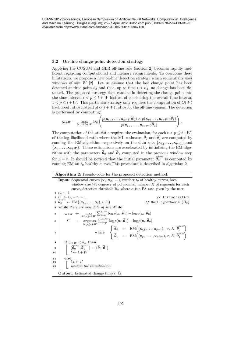
3.2 On-line change-point detection strategyApplying the CUSUM and GLR off-line rule (section 2) becomes rapidly inef-ficient regarding computational and memory requirements. To overcome theselimitations, we propose a new on-line detection strategy which sequentially useswindows of size W [2]. Let us assume that the last change point has beendetected at time point tA and that, up to time t > tA, no change has been de-tected. The proposed strategy then consists in detecting the change point intothe time interval t < p ≤ t+W instead of considering the overall time interval1 < p ≤ t+W . This particular strategy only requires the computation of O(W )likelihood ratios instead of O(t+W ) ratios for the off-line version. The detectionis performed by computing:

gt+W = maxt<p≤t+W

log(p(xtA

, . . . ,xp−1; θ0)× p(xp, . . . ,xt+W ; θ1)p(xtA

, . . . ,xt+W ; θ0)

).

The computation of this statistic requires the evaluation, for each t < p ≤ t+W ,of the log likelihood ratio where the ML estimates θ0 and θ1 are computed byrunning the EM algorithm respectively on the data sets {xtA

, . . . ,xp−1} and{xp, . . . ,xt+W }. These estimations are accelerated by initializing the EM algo-rithm with the parameters θ0 and θ1 computed in the previous window stepfor p = t. It should be noticed that the initial parameter θ

init

0 is computed byrunning EM on t0 healthy curves.This procedure is described in algorithm 2.

Algorithm 2: Pseudo-code for the proposed detection method.Input: Sequential curves (x1,x2, . . . ), number t0 of healthy curves, local

window size W , degree r of polynomial, number K of segments for eachcurve, detection threshold hα where α is a FA rate given by the user

1 tA ← 12 t ← tA + t0 − 1 // Initialization3 θ

init

0 ← EM((xtA , . . . ,xt), r,K

)// Null hypothesis (H0)

4 while there are new data of size W do5 gt+W ← max

t<p≤t+W

∑t+Wi=p log p(xi; θ1)− log p(xi; θ0)

6 t∗ ← arg maxt<p≤t+W

∑t+Wi=p log p(xi; θ1)− log p(xi; θ0)

7 where

θ0 ← EM(

(xtA , . . . ,xp−1), r, K, θinit

0

)θ1 ← EM

((xp, . . . ,xt+W ), r, K, θ

init

1

)8 if gt+W < hα then9 (θ

init

0 , θinit

1 )← (θ0, θ1)10 t← t+W

11 else12 tA ← t∗

13 Restart the initialization

Output: Estimated change time(s) tA

402


4 Experimental studies

Opening and closing operations have a similar behavior ; in this article, we onlyreport results related to door closing operations. The dataset has been recordedin July 2011 on a 18-meters articulated bus. Two variables were recorded: thepressure inside door pneumatic actuators and the door position. A samplingfrequency of 100Hz was adopted. The resulting curves length was m = 204.

The number of curves needed to learn θinit

0 was set to 10 and the windowsize W was set to 5 curves. We have observed that the window size does notaffect the detection quality but can slow down the process if too large.

Relevant hyperparameters embedded in the density estimation model, aredetermined using a physical prior i.e. K = 3, which corresponds to the threesteps during the door operation (Fig. 1); the degree r of polynomial regressionmodel was experimentally set to 4.

The detection threshold, based on α (the expected false alarm rate providedby the user), is estimated as follows: first, the multivariate RHLP is used tolearn a parameter vector θ0 on a set of healthy closing operation curves ; then,curves sequences of size 15 000 are generated from distribution p(xi;θ0); finally,the threshold is formed by the (1 − α) confidence interval of the test statistic.In this article, α was set to 0.1, 0.01 and 0.001.

Two performance metrics were used to evaluate the proposed method: thefalse alarm rate (FAR) and the average detection delay (ADD) that is to saythe delay to detect an effective degraded curve after the change point. Notethat FAR is computed on the healthy curves. Each curves sequence consists of10 250 curves including 10 000 defect-free curves and 250 curves correspondingto a door blocking damage.

−6.9 −4.6 −2.3−6.9

−4.6

−2.3

log(α)

log(

FA

R)

Noise level=10Noise level=30Noise level=50α

2 10 20 30 40 500

5

10

15

20

25

30

35

Noise level

AD

D

α=0.001α=0.010α=0.100

Fig. 2: log(α) VS log(FAR) (left). And impact of the noise level on detection delay(right). Each value of log(FAR) and ADD is an average over 10 different sequences.

Figure 2 (left) displays the logarithm of FAR as a function of the logarithmof α. We observe that FAR indicator is stable for the different values of noiselevel. In fact, similar values between FAR and α means that the detectionthreshold has been correctly estimated. Figure 2 (right) shows the behaviorof ADD in relation with the noise level which is a multiplicative factor of thevariance Σk. It can be seen that ADD increases with the noise level and that nochange is detected when the noise level is too large (distribution before changeand distribution after change are overlapping).

403


46

8100

200300

0

0.5

1

Pressure (bar)Time

Pos

ition

0 50 100 150 200 250 3000

50

100

150

200

250

300

t

Clo

sing

sta

tistic

h

0.001=33.4642

Fig. 3: Example of detection on closing curves (α is set to 0.001 and noise level is setto 2). 200 in-control observations are in blue and 100 anomalies in red (left); statisticgt is in blue, estimated detection threshold is in red and alarm is the red circle (right).

5 ConclusionIn this paper, we have presented a sequential method to detect anomalies ina curves sequence. The proposed method uses a CUSUM-like test based ondensities defined on the curves space. This approach is suitable for suddenchanges, like in operating system breakdown. A generative model has beendefined for density estimation which is a multivariate extension of the HiddenProcess Regression Model [3]. This strategy is applied to monitor pneumaticdoors. The experimental results showed a certain practicability of the approach.We believe this strategy could be used to an application when sustained specialcauses are observed, those that continue until they are identified and fixed.

References[1] M. Basseville and I. Nikiforov. Detection of Abrupt Changes: Theory and Applications.

Prentice-Hall, Englewood Cliffs, NJ, USA, 1993.[2] T. Lai. Sequential analysis: some classical problems and new challenges. Statist. Sinica,

11(2):303–408, 2001.[3] F. Chamroukhi, A. Same, G. Govaert, and P. Aknin. A hidden process regression model for

functional data description. Application to curve discrimination. Neurocomputing, 73(7-9):1210–1221, March 2010.

[4] G. Lorden. Procedures for Reacting to a Change in Distribution. The Annals of Mathe-matical Statistics, 42(6), 1971.

[5] G. Moustakides. Optimal Stopping Times for Detecting Changes in Distributions. TheAnnals of Statistics, 14(4):1379–1387, 1986.

[6] A. P. Dempster, N. M. Laird, and D. B. Rubin. Maximum Likelihood from Incomplete Datavia the EM Algorithm. Journal of the Royal Statistical Society. Series B (Methodological),39(1):1–38, 1976.

[7] P. Green. Iteratively reweighted least squares for maximum likelihood estimation,and somerobust and resistant alternatives. Journal of the Royal Statistical Society B, 46:149–192,2003.

404


a cusum approach for online change-point detection … · a cusum approach for online change-point...

Documents