A Comparison of Two SVAR Studies

with Long-Run Restrictions

Atilim Seymen

University of Hamburg

Economics Department

Von-Melle-Park 5, IWK

D-20146 Hamburg, Germany

E-mail: seymen@econ.uni-hamburg.de

This Version: October 15, 2006

Preliminary: Do not cite without author’s permisson.

JEL classification: C32, C51, C52

Keywords: Structural Vector Autoregression Models, Long-Run Restrictions, Macroeconomic

Shocks, Business Cycles, Error Variance Decomposition

An earlier version of this paper was presented in two seminars at Ege University and Izmir

University of Economics in Izmir, and at the 4th PhD Conference in Economics in Volterra. I

thank to the participants of these events and my colleagues Beatriz Gaitan and Olaf Posch, from the

Institute for Growth and Business Cycles of the University of Hamburg for their helpful comments.

1

1 Introduction

This paper compares two seminal macroeconometric studies by King, Plosser, Stock and Watson

(1991; henceforth KPSW) and Gali (1999) who use the structural vector autoregression (SVAR)

technique with long-run restrictions in order to identify macroeconomic shocks and investigate the

sources of business cycle fluctuations. As noted by Faust and Leeper (1997), checking for consistency

of results across various small SVAR models can help to maintain the convenience of small models.

If two different SVAR models come to similar results the researcher finds a clear support for the

reliability of his results. If different SVAR models, on the other hand, come to different conclusions

about the same question, the researcher needs a deeper analysis of his models1. Obviously, at

most one of the models can be correct in such a case. In this paper, we investigate the findings of

different SVAR models. The models differ in the way identification occurs as well as in terms of

the variables included in the VAR.

The investigation in our paper is closely related to the findings of Alexius and Carlsson (2005,

2001) who study to what extent structural VAR models are capable of capturing the phenomena

that they are supposed to capture. They basically compare the technology shocks identified using

the bivariate Gali and KPSW models with different technology measures that are computed using

the production function approach: The first measure is the conventional Solow residual and the

second is the refined Solow residual that is considered by Basu and Kimball (1997) inter alia.

According to their findings, the technology measures of the three-variable and six-variable KPSW

models do not reflect shocks to technology, but the technology measures resulting from the bivariate

Gali model. The technology measure derived from the KPSW model mixes technology shocks with

nontechnology phenomena. The Gali model, on the other hand, appears to be much more robust to

nontechnology measures, as Alexius and Carlsson (2005) note.

We augment the bivariate model of Gali in the way as it is suggested in his study, that is, we add

real balances, real interest and inflation to his bivariate VAR that contains only labor productivity

and labor input. Thus, the five-variable Gali and the six-variable KPSW models have output, real

balances and nominal interest rate as the common variables. In order to provide a consistency

between these models, we check the impact of assuming a long-run money-demand relationship

1To give an example, the technology shock of the three-variable KPSW model, the real interest shock of the

six-variable KPSW model and the nontechnology shock of the bivariate Gali model considered in this paper all seem

to refer to a similar phenomenon. The researcher faces then the problem of how to call the identified mechanism:

Technology, nontechnology, or real interest?

2

in the Gali model like in the KPSW model. Note that there should be at least one cointegrating

relationship in the five-variable Gali model and only four permanent shocks if a long-run money-

demand relationship is existent. We name these permanent shocks technology, labor supply, real

interest and inflation and put them into comparison with the technology, real interest and inflation

shocks of KPSW.

The results in the study by Alexius and Carlsson (2005) underline the importance of the absence

of a labor input variable in KPSW models. Labor input is used as a proxy for capacity utilization

when computing the refined Solow residual and containing it in a VAR that aims at identifiying the

technology shocks seems to help against the mixing of technology and nontechnology phenomena.

The KPSW models possess an omitted variables bias due to the lack of labor input in the VAR

whereas the Gali model does not, at least not with respect to the identification of technology shocks.

We report the consequences of augmenting the three- and six-variable KPSW models with labor

input.

We consider next the refinement of the structural shocks identified by the SVAR models con-

sidered. This is done by adding the first-differences of oil price and national defense expenditures

as exogenous variables to the VARs. Alexius and Carlsson (2005) have already shown that the first

differences of these two measures are orthogonal to both KPSW and Gali technology measures2.

Finally, we propose a novel variance decomposition approach in order to compute the role of

structural shocks in the business cycle fluctuations of the macroeconomic variables. Technology

shocks are in none of the augmented models considered the driving force of the business cycle fluc-

tuations. A surprising result is that supply, in particular labor supply, shocks play the biggest role

in the fluctuations of real balances, but not the monetary shocks, namely real-interest and inflation

shocks. Consumption and investment fluctuations are mainly monetary phenomena whereas the

role of technology shocks in these fluctuations is marginal.

The next section briefly reviews the two identification schemes considered throughout this paper.

We discuss the basic models in Section 3 and compare them. Section 4 is devoted to the modification

of the basic models. The following section deals with the question of which shocks explain the

business cycle fluctuations of the macroeconomic variables. Section 6 concludes.

2Alexius and Carlsson (2005) work with the three-variable KPSW and bivariate Gali models.

3

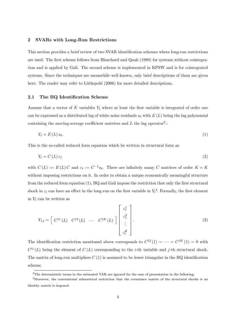
2 SVARs with Long-Run Restrictions

This section provides a brief review of two SVAR identification schemes where long-run restrictions

are used. The first scheme follows from Blanchard and Quah (1989) for systems without cointegra-

tion and is applied by Gali. The second scheme is implemented in KPSW and is for cointegrated

systems. Since the techniques are meanwhile well-known, only brief descriptions of them are given

here. The reader may refer to Lutkepohl (2006) for more detailed descriptions.

2.1 The BQ Identification Scheme

Assume that a vector of K variables Yt where at least the first variable is integrated of order one

can be expressed as a distributed lag of white noise residuals ut with E (L) being the lag polynomial

containing the moving-average coefficient matrices and L the lag operator3.:

Yt = E (L)ut. (1)

This is the so-called reduced form equation which be written in structural form as

Yt = C (L) εt (2)

with C (L) := E (L)C and εt := C−1ut. There are infinitely many C matrices of order K ×Kwithout imposing restrictions on it. In order to obtain a unique economically meaningful structure

from the reduced form equation (1), BQ and Gali impose the restriction that only the first structural

shock in εt can have an effect in the long-run on the first variable in Yt4. Formally, the first element

in Yt can be written as

Y1,t =hC11 (L) C12 (L) · · · C1K (L)

i

ε1t

ε2t...

εKt

. (3)

The identification restriction mentioned above corresponds to C12 (1) = · · · = C1K (1) = 0 with

Cij (L) being the element of C (L) corresponding to the i-th variable and j-th structural shock.

The matrix of long-run multipliers C (1) is assumed to be lower triangular in the BQ identification

scheme.

3The deterministic terms in the estimated VAR are ignored for the ease of presentation in the following.4Moreover, the conventional atheoretical restriction that the covariance matrix of the structural shocks is an

identity matrix is imposed.

4

2.2 The KPSW Identification Scheme

The identification scheme developed by KPSW is applied to VAR systems with cointegrated vari-

ables5. The matrix of long-run multipliers can be written as

Γ (1) =hA 0

i(4)

where Γ (1) is analogous to C (1), A is of order K × k and 0 is the zeros matrix of order K × r, kbeing the number of stochastic trends and r the cointegration rank. Furthermore, the matrix A is

assumed to have the form

A = AΠ (5)

where A is a known K×k matrix and Π is a k×k lower triangular matrix with ones on its diagonal.KPSW construct the A matrix by using the parameters of the cointegrating equations which are

estimated with the dynamic OLS technique. As Jang and Ogaki (2001) show, A can be determined

by exploiting the fact that β0A = 0 and β0β⊥ = 0 must be valid, where β is the K × r matrix ofcointegrating vectors and β⊥ is its orthogonal with the order K × k. Thus, one can choose

A = β⊥. (6)

This means that where the cointegrating vectors are estimated there are some free parameters in

the matrix A which are not restricted other than β0β⊥ = 0. Notice that the number of unrestricted

parameters in β⊥ can be r times k, i.e., the cointegration rank times the number of stochastic

trends in the VAR6.

3 The Basic Models

We discuss the nature of the results in basic Gali and KPSW models in this section. Original data

is used when generating the results7. In the following, a one-standard-deviation structural shock

is always considered when plotting the dynamic responses. The business cycle component with

respect to (w.r.t.) a certain structural shock means that all the other shocks are set to zero in the

SVAR when the historical time series are computed and the result is HP-filtered.

5The notation in Jang and Ogaki (2001) is used here while describing the KPSW identification scheme.6This follows from the fact that the matrix β0β⊥ has the order r × k.7I thank Professor Gali for providing me with his original data. The original KPSW data can be found on the file

http://www.wws.princeton.edu/˜mwatson/ddisk/kpsw.zip.

5

3.1 Gali (1999)

The main model in Gali (1999) is a bivariate VAR containing labor productivity, x, and labor

input, n. Both variables are nonstationary according to the Augmented Dickey-Fuller (ADF) test,

but not cointegrated. The crucial identifying restriction is that the technology shock is the only

structural shock that has an impact on labor productivity in the long-run.

The so-called omitted variables bias can be a relevant issue in particular for bivariate SVAR

models. If some variables that are important for the explanation of the particular macroeconomic

issue investigated are left out, the identification scheme may not even be approximately correct.

Gali (1999) augments his bivariate model with the first-differences of three more variables, namely

real balances, m− p, real interest rate8, R −∆p, and inflation, ∆p. Gali illustrates the responsesto a technology shock in the five-variable model in Figure 4 of his paper and points to similarities

to the bivariate case. A comparison of the identified technology9 shocks, dynamic responses to a

technology shock and technology component of the model variables shows that omitted variables

bias is not an important issue for the bivariate model, i.e., the bivariate model seems to be a

good approximation for the research question posed in Gali (1999): Do technology shocks explain

aggregate fluctuations? The result is that technology shocks are clearly not the driving force

behind the aggregate fluctuations. We find that the identified technology shocks in bivariate and

five-variable models are correlated with a coefficient of 0.92. The output technology cycles are

correlated with a coefficient of 0.66 and the labor input technology cycles with a coefficient of

0.78. The correlation coefficients of the nontechnology business cycle components of output, labor

productivity and labor input are 0.97, 0.96 and 0.92, respectively10.

Figure 1 illustrates the responses of output, labor input and labor productivity in bivariate and

five-variable models. We notice that augmenting the model with three additional variables does not

create a difference in the short-run, namely one-year, dynamic responses of output and labor input,

however in the mid- and long-run it does11. The qualitative patterns of the dynamic responses of

8The real interest rate enters the VAR in level in Gali (1999). However, we assume this variable to be I (1) in this

paper in order to be consistent with KPSW. A sensitivity analysis shows that the results do not change significantly

because of this assumption.9Only the technology shocks and their components are considered. Note that the five-variable model does not

identify the four nontechnology shocks seperately. So, it does not make sense to compare the demand shocks of the

bivariate model with the unidentified demand shocks of the five-variable model.10The four nontechnology components of a certain variable are added up for computing the nontechnology business

cycle component of it in the five-variable model.11This is basically the reason behind the relatively lower correlations of output and labor input technology cycles

6

The Response to a Technology Shock

Bivariate Model (solid), Five-Variable Model (dashed)

y: output, n: labor input, x: labor productivity

Figure 1: Dynamic Responses in the Bivariate and Five-Variable Gali Models

these variables do not change though. Nevertheless, the long-run effect of a technology shock on

labor input becomes positive when the bivariate model is augmented. Overall, the critique of Faust

and Leeper (1997) applies to output and labor input, but not to labor productivity12. That is, we

would expect small changes in the model parameters to cause big changes in the long-run effects

of shocks, but this does not happen to be the case for labor productivity as Figure 1 shows.

3.2 King et al. (1991)

KPSW investigate a three-variable and a six-variable model with long-run restrictions. The dif-

ference to the identification scheme above is that the model variables considered in KPSW are

cointegrated. The three-variable model consists of output, y, consumption, c, and investment, i. It

is augmented later with real balances, m−p, nominal interest rate, R, and inflation, ∆p. The testspoint to a cointegration rank of one in the three-variable model, and three in the six-variable model.

A comparison of Figures 2 and 4 in KPSW makes it clear that augmenting the three-variable model

leads to important changes in the results with respect to the identified technology shocks.

Cointegration and identification We skip the three-variable case and consider immediately the

six-variable model in the following. KPSW make use of the estimated cointegrating relationships

while determining the shape of the A matrix given in equation (5). In Table 2 of their paper, they

report the results of three estimated cointegrating relationships in the six-variable system. The

in comparison to labor productivity technology cycles.12Notice that it seems as if the dynamic responses of labor productivity are sensitive in the short-run in Figure 1,

but this is not so. The scale of the y axis in the graph of the labor productivity response is just too small.

7

first is the money demand equation,

m− p = βyy − βRR, (7)

and the other two are relationships between the real ratios and the real interest:

c− y = φ1 (R−∆p) (8)

and

i− y = φ2 (R−∆p) . (9)

βy, βR, φ1 and φ2 are coefficients. The A matrix in the matrix of long-run multipliers Γ (1) is given

by

A =

1 0 0

1 0 φ1

1 0 φ2

βy −βR −βR0 1 1

0 1 0

1 0 0

π21 1 0

π31 π32 1

, (10)

or

A =

1 0 0

1 + φ1π31 φ1π32 φ1

1 + φ2π31 φ2π32 φ2

βy − βRπ21 − βRπ31 −βR (1− π32) −βRπ21 + π31 1 + π32 1

π21 1 0

. (11)

The order of the variables in the model is y, c, i,m − p,R,∆p. Notice that the A matrix in

(10) is written such that the long-run relationships given in equations (7) , (8) and (9) hold13.

13Consider, for example, what happens to (8) in the long-run when a one-time one unit balanced-growth shock

occurs. One can express the change in (8) as

∆c−∆y = φ1¡∆R−∆2p

¢(12)

with ∆c = 1 + φ1π31, ∆y = 1, ∆R = π21 + π31 and ∆2p = π21 which follow from equation (11) . It is seen that (12)

holds when these values are substituted in. This phenomenon is indeed valid for all the cointegrating relationships

and all the three permanent shocks.

8

Furthermore, A is orthogonal to the cointegrating vectors that would come from (7) , (8) and (9) 14.

KPSW call the first shock a real-balanced-growth (technology) shock and indicate that it leads

to a unit long-run increase in y, c, and i. This is, however, not true as can be detected from (11).

The long-run effect of a “balanced-growth” shock is 1, 1 + φ1π31, and 1 + φ2π31 on y, c, and i,

respectively15. Hence, ∆c −∆y = φ1π31 in the long run, but not ∆c −∆y = 0. The second andthird permanent shocks are respectively called inflation and real interest shocks by KPSW and they

also lead to ∆c−∆y 6= 0.Equation (11) tells that output can be affected by only the balanced-growth shock in the long

run. Inflation shock is the second permanent shock since it has a unit effect on the inflation rate in

the long run. Finally, the reason to call the last shock a “real interest shock” is that it has a unit

impact on the real interest, R−∆p, in the long run16.

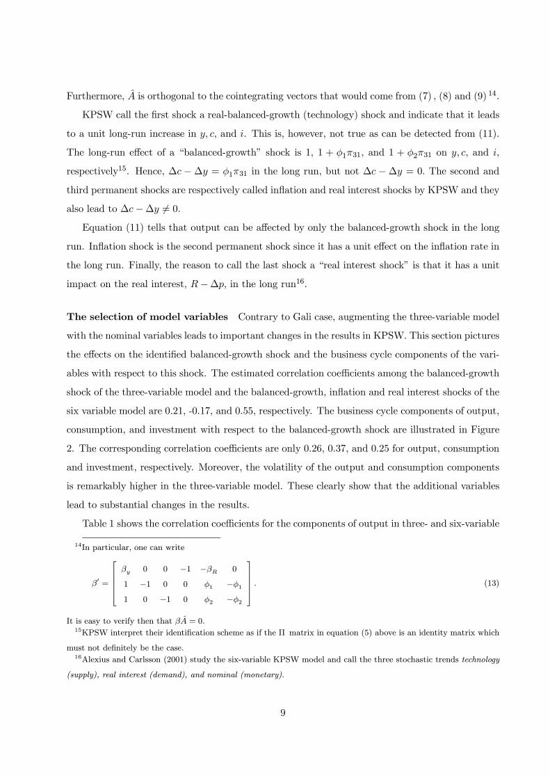
The selection of model variables Contrary to Gali case, augmenting the three-variable model

with the nominal variables leads to important changes in the results in KPSW. This section pictures

the effects on the identified balanced-growth shock and the business cycle components of the vari-

ables with respect to this shock. The estimated correlation coefficients among the balanced-growth

shock of the three-variable model and the balanced-growth, inflation and real interest shocks of the

six variable model are 0.21, -0.17, and 0.55, respectively. The business cycle components of output,

consumption, and investment with respect to the balanced-growth shock are illustrated in Figure

2. The corresponding correlation coefficients are only 0.26, 0.37, and 0.25 for output, consumption

and investment, respectively. Moreover, the volatility of the output and consumption components

is remarkably higher in the three-variable model. These clearly show that the additional variables

lead to substantial changes in the results.

Table 1 shows the correlation coefficients for the components of output in three- and six-variable

14In particular, one can write

β0 =

βy 0 0 −1 −βR 0

1 −1 0 0 φ1 −φ11 0 −1 0 φ2 −φ2

. (13)

It is easy to verify then that βA = 0.15KPSW interpret their identification scheme as if the Π matrix in equation (5) above is an identity matrix which

must not definitely be the case.16Alexius and Carlsson (2001) study the six-variable KPSW model and call the three stochastic trends technology

(supply), real interest (demand), and nominal (monetary).

9

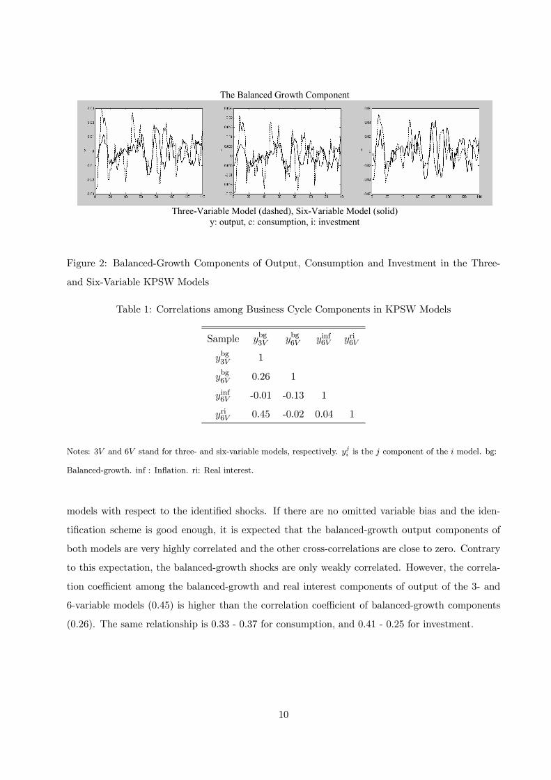
The Balanced Growth Component

Three-Variable Model (dashed), Six-Variable Model (solid)

y: output, c: consumption, i: investment

Figure 2: Balanced-Growth Components of Output, Consumption and Investment in the Three-

and Six-Variable KPSW Models

Table 1: Correlations among Business Cycle Components in KPSW Models

Sample ybg3V ybg6V yinf6V yri6V

ybg3V 1

ybg6V 0.26 1

yinf6V -0.01 -0.13 1

yri6V 0.45 -0.02 0.04 1

Notes: 3V and 6V stand for three- and six-variable models, respectively. yji is the j component of the i model. bg:

Balanced-growth. inf : Inflation. ri: Real interest.

models with respect to the identified shocks. If there are no omitted variable bias and the iden-

tification scheme is good enough, it is expected that the balanced-growth output components of

both models are very highly correlated and the other cross-correlations are close to zero. Contrary

to this expectation, the balanced-growth shocks are only weakly correlated. However, the correla-

tion coefficient among the balanced-growth and real interest components of output of the 3- and

6-variable models (0.45) is higher than the correlation coefficient of balanced-growth components

(0.26). The same relationship is 0.33 - 0.37 for consumption, and 0.41 - 0.25 for investment.

10

3.3 The Comparison of Different Models

Note that all models considered up to this point contain output17 and technology (balanced-growth)

shocks. Therefore, it is natural to investigate first if the estimated technology shocks and the

corresponding business cycle components of output are connected to each other. The technology

shocks are already investigated by Alexius and Carlsson (2005, 2001). Therefore, we skip this task

in this paper. The second important issue is the orthogonality of different structural shocks across

the models. If different structural shocks are not approximately orthogonal to each other, this

would be a sign for a lot of noise in the data and the researcher should take care when extracting

information from the models. Five different models are compared from different viewpoints in this

subsection: KPSW3V, KPSW6V, Gali2V and Gali5V18, that is, the three- and six-variable KPSW,

and bivariate and five-variable Gali models.

Obviously, a coherent data set is needed if one wants to make consistent comparisons. For

this reason, the original KPSW data is taken as the underlying data for the common variables19.

The labor input measure of Gali follows from the original paper. The common sample period is

1954:1-1988:4.

A consistent selection of the lag number seems to be problematic in the literature20. KPSW

use eight lags and Gali four lags in their estimated VAR models. We use four lags in the bivariate

Gali model and eight lags in the others.

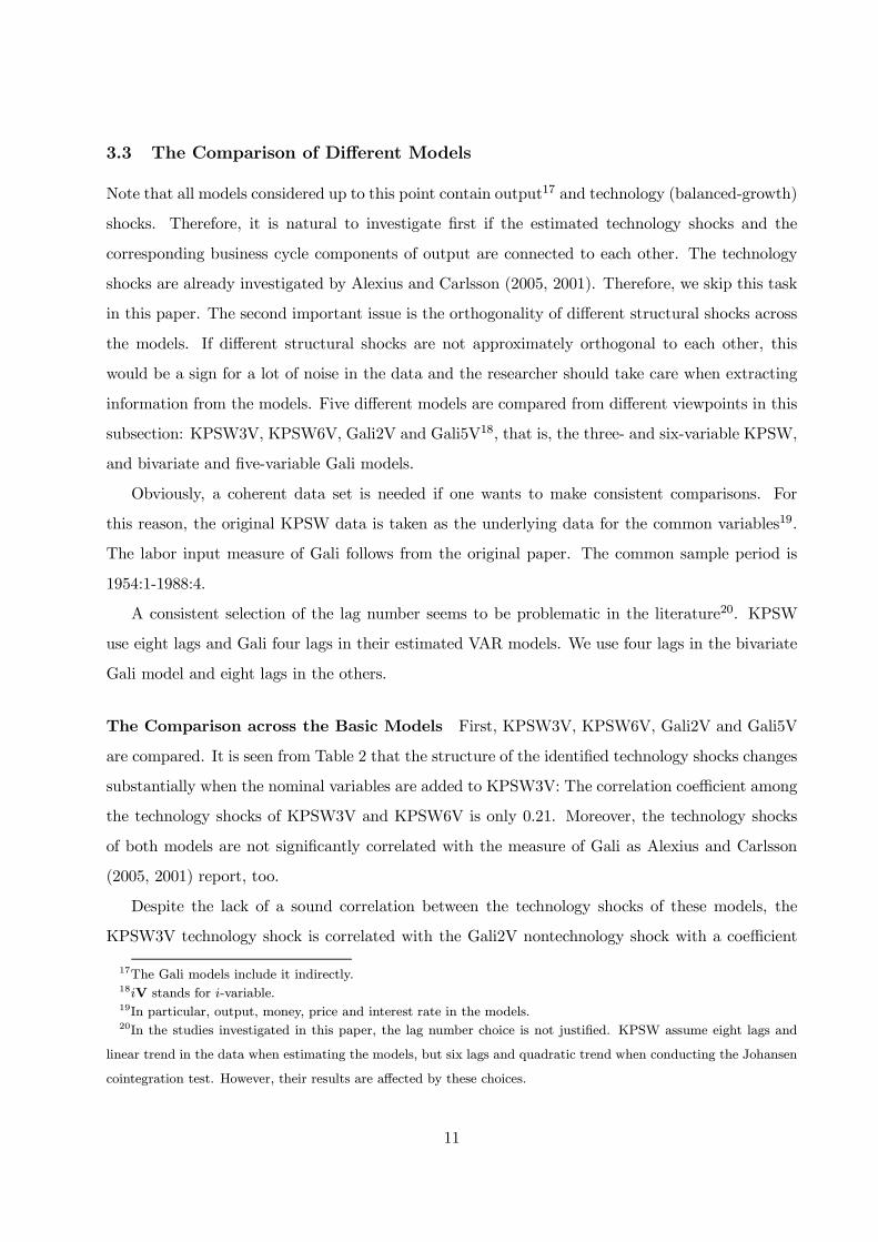
The Comparison across the Basic Models First, KPSW3V, KPSW6V, Gali2V and Gali5V

are compared. It is seen from Table 2 that the structure of the identified technology shocks changes

substantially when the nominal variables are added to KPSW3V: The correlation coefficient among

the technology shocks of KPSW3V and KPSW6V is only 0.21. Moreover, the technology shocks

of both models are not significantly correlated with the measure of Gali as Alexius and Carlsson

(2005, 2001) report, too.

Despite the lack of a sound correlation between the technology shocks of these models, the

KPSW3V technology shock is correlated with the Gali2V nontechnology shock with a coefficient

17The Gali models include it indirectly.18iV stands for i-variable.19In particular, output, money, price and interest rate in the models.20In the studies investigated in this paper, the lag number choice is not justified. KPSW assume eight lags and

linear trend in the data when estimating the models, but six lags and quadratic trend when conducting the Johansen

cointegration test. However, their results are affected by these choices.

11

Table 2: Correlations among the Identified Technology Shocks

Model KPSW3V KPSW6V Gali2V Gali5V Gali5V1

KPSW3V 1

KPSW6V 0.21 1

Gali2V 0.14 0.17 1

Gali5V 0.15 0.06 0.90 1

Gali5V1 0.01 0.35 0.82 0.79 1

Notes: Correlations among the identified technology shocks of KPSW3V, KPSW6V, Gali2V and BQ2V models.

Figure 3: Dynamic Responses of Output

of 0.57. Moreover, it is correlated with the KPSW6V real interest shock with a coefficient of 0.61.

It may therefore be concluded that what is presented as a technology measure in KPSW3V, i.e.,

the balanced-growth shock, and the real-interest shock in KPSW6V contain substantial nontech-

nology and/or demand elements. The illustration of the dynamic responses in Figure 3 endorses

this interpretation. Although there are important quantitative discrepancies among the dynamic

responses, they all follow similar patterns. Furthermore, note that these technology, real interest

and nontechnology shocks are reported to be the main driving force behind the business cycle

fluctuations in the corresponding papers. Hence, we think that, although with some bias, they

point to a similar phenomenon. Taking into account the bias that the respective KPSW3V and

KPSW6V technology and real interest measures represent indeed nontechnology phenomena, we

come to the same conclusion with all the models which is that the nontechnology shocks play the

more important role behind the business cycle fluctuations.

12

Cointegration Properties of Gali5V and KPSW6V Gali checks the robustness of his results

with an augmented model. Notice that there are four common variables of KPSW6V and Gali5V:

output, real balances, real interest rate and inflation21. Although Gali reports no cointegration in

his data set, KPSW do. The real ratio relationships do obviously not exist in the Gali model, but

at least the money demand relation must exist if KPSW are right. It is unfortunately the case

that one cannot easily come to a conclusion about the cointegration rank in KPSW. For some test

specifications, it is possible that KPSW6V has a cointegration rank of only two and there is no a

priori reason not to assume that these two relationships are the great ratios. Then, it would not

make sense to assume a long-run money-demand relationship in Gali5V22. But if a cointegration

rank of three is assumed in KPSW6V and the third relationship to be the money-demand equation,

Gali5V should also have a cointegration rank of at least one.

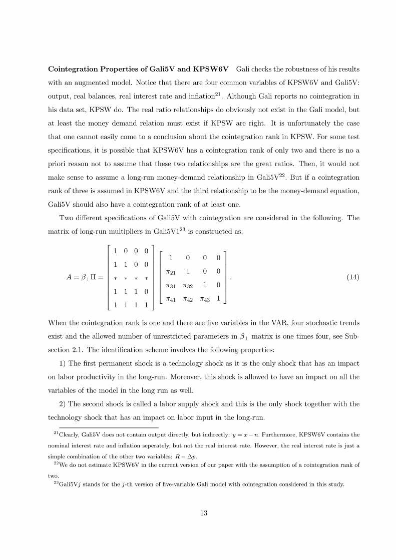
Two different specifications of Gali5V with cointegration are considered in the following. The

matrix of long-run multipliers in Gali5V123 is constructed as:

A = β⊥Π =

1 0 0 0

1 1 0 0

∗ ∗ ∗ ∗1 1 1 0

1 1 1 1

1 0 0 0

π21 1 0 0

π31 π32 1 0

π41 π42 π43 1

. (14)

When the cointegration rank is one and there are five variables in the VAR, four stochastic trends

exist and the allowed number of unrestricted parameters in β⊥ matrix is one times four, see Sub-

section 2.1. The identification scheme involves the following properties:

1) The first permanent shock is a technology shock as it is the only shock that has an impact

on labor productivity in the long-run. Moreover, this shock is allowed to have an impact on all the

variables of the model in the long run as well.

2) The second shock is called a labor supply shock and this is the only shock together with the

technology shock that has an impact on labor input in the long-run.

21Clearly, Gali5V does not contain output directly, but indirectly: y = x− n. Furthermore, KPSW6V contains thenominal interest rate and inflation seperately, but not the real interest rate. However, the real interest rate is just a

simple combination of the other two variables: R−∆p.22We do not estimate KPSW6V in the current version of our paper with the assumption of a cointegration rank of

two.23Gali5Vj stands for the j-th version of five-variable Gali model with cointegration considered in this study.

13

3) The third permanent shock is a real interest shock in the spirit of KPSW which affects the

real interest rate by one unit in the long run.

4) The fourth permanent shock is an inflation shock which can affect only the inflation rate in

the long run, but not the real variables except the real balances.

5) The only transitory shock is not given an economic interpretation like in KPSW24.

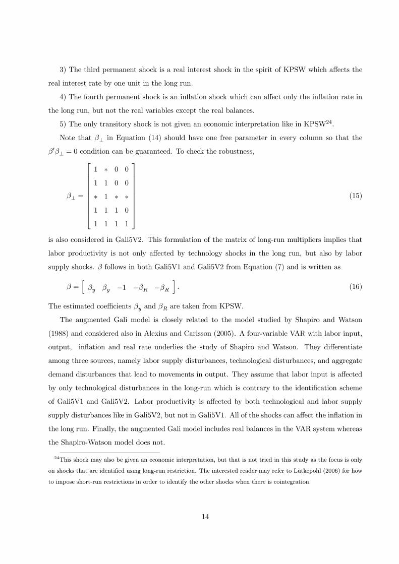
Note that β⊥ in Equation (14) should have one free parameter in every column so that the

β0β⊥ = 0 condition can be guaranteed. To check the robustness,

β⊥ =

1 ∗ 0 0

1 1 0 0

∗ 1 ∗ ∗1 1 1 0

1 1 1 1

(15)

is also considered in Gali5V2. This formulation of the matrix of long-run multipliers implies that

labor productivity is not only affected by technology shocks in the long run, but also by labor

supply shocks. β follows in both Gali5V1 and Gali5V2 from Equation (7) and is written as

β =hβy βy −1 −βR −βR

i. (16)

The estimated coefficients βy and βR are taken from KPSW.

The augmented Gali model is closely related to the model studied by Shapiro and Watson

(1988) and considered also in Alexius and Carlsson (2005). A four-variable VAR with labor input,

output, inflation and real rate underlies the study of Shapiro and Watson. They differentiate

among three sources, namely labor supply disturbances, technological disturbances, and aggregate

demand disturbances that lead to movements in output. They assume that labor input is affected

by only technological disturbances in the long-run which is contrary to the identification scheme

of Gali5V1 and Gali5V2. Labor productivity is affected by both technological and labor supply

supply disturbances like in Gali5V2, but not in Gali5V1. All of the shocks can affect the inflation in

the long run. Finally, the augmented Gali model includes real balances in the VAR system whereas

the Shapiro-Watson model does not.

24This shock may also be given an economic interpretation, but that is not tried in this study as the focus is only

on shocks that are identified using long-run restriction. The interested reader may refer to Lutkepohl (2006) for how

to impose short-run restrictions in order to identify the other shocks when there is cointegration.

14

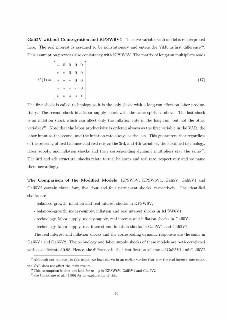
Gali5V without Cointegration and KPSW6V1 The five-variable Gali model is reinterpreted

here. The real interest is assumed to be nonstationary and enters the VAR in first difference25.

This assumption provides also consistency with KPSW6V. The matrix of long-run multipliers reads

C (1) =

∗ 0 0 0 0

∗ ∗ 0 0 0

∗ ∗ ∗ 0 0

∗ ∗ ∗ ∗ 0

∗ ∗ ∗ ∗ ∗

. (17)

The first shock is called technology as it is the only shock with a long-run effect on labor produc-

tivity. The second shock is a labor supply shock with the same spirit as above. The last shock

is an inflation shock which can affect only the inflation rate in the long run, but not the other

variables26. Note that the labor productivity is ordered always as the first variable in the VAR, the

labor input as the second, and the inflation rate always as the last. This guarantees that regardless

of the ordering of real balances and real rate as the 3rd, and 4th variables, the identified technology,

labor supply, and inflation shocks and their corresponding dynamic multipliers stay the same27.

The 3rd and 4th structural shocks relate to real balances and real rate, respectively and we name

them accordingly.

The Comparison of the Modified Models KPSW6V, KPSW6V1, Gali5V, Gali5V1 and

Gali5V2 contain three, four, five, four and four permanent shocks, respectively. The identified

shocks are

- balanced-growth, inflation and real interest shocks in KPSW6V;

- balanced-growth, money-supply, inflation and real interest shocks in KPSW6V1;

- technology, labor supply, money-supply, real interest and inflation shocks in Gali5V;

- technology, labor supply, real interest and inflation shocks in Gali5V1 and Gali5V2.

The real interest and inflation shocks and the correspoding dynamic responses are the same in

Gali5V1 and Gali5V2. The technology and labor supply shocks of these models are both correlated

with a coefficient of 0.98. Hence, the difference in the identification schemes of Gali5V1 and Gali5V2

25Although not reported in this paper, we have shown in an earlier version that how the real interest rate enters

the VAR does not affect the main results.26This assumption is does not hold for m− p in KPSW6V, Gali5V1 and Gali5V2.27See Christiano et al. (1999) for an explanation of this.

15

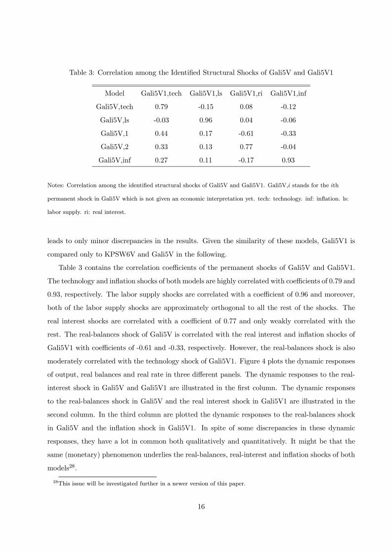
Table 3: Correlation among the Identified Structural Shocks of Gali5V and Gali5V1

Model Gali5V1,tech Gali5V1,ls Gali5V1,ri Gali5V1,inf

Gali5V,tech 0.79 -0.15 0.08 -0.12

Gali5V,ls -0.03 0.96 0.04 -0.06

Gali5V,1 0.44 0.17 -0.61 -0.33

Gali5V,2 0.33 0.13 0.77 -0.04

Gali5V,inf 0.27 0.11 -0.17 0.93

Notes: Correlation among the identified structural shocks of Gali5V and Gali5V1. Gali5V,i stands for the ith

permanent shock in Gali5V which is not given an economic interpretation yet. tech: technology. inf: inflation. ls:

labor supply. ri: real interest.

leads to only minor discrepancies in the results. Given the similarity of these models, Gali5V1 is

compared only to KPSW6V and Gali5V in the following.

Table 3 contains the correlation coefficients of the permanent shocks of Gali5V and Gali5V1.

The technology and inflation shocks of both models are highly correlated with coefficients of 0.79 and

0.93, respectively. The labor supply shocks are correlated with a coefficient of 0.96 and moreover,

both of the labor supply shocks are approximately orthogonal to all the rest of the shocks. The

real interest shocks are correlated with a coefficient of 0.77 and only weakly correlated with the

rest. The real-balances shock of Gali5V is correlated with the real interest and inflation shocks of

Gali5V1 with coefficients of -0.61 and -0.33, respectively. However, the real-balances shock is also

moderately correlated with the technology shock of Gali5V1. Figure 4 plots the dynamic responses

of output, real balances and real rate in three different panels. The dynamic responses to the real-

interest shock in Gali5V and Gali5V1 are illustrated in the first column. The dynamic responses

to the real-balances shock in Gali5V and the real interest shock in Gali5V1 are illustrated in the

second column. In the third column are plotted the dynamic responses to the real-balances shock

in Gali5V and the inflation shock in Gali5V1. In spite of some discrepancies in these dynamic

responses, they have a lot in common both qualitatively and quantitatively. It might be that the

same (monetary) phenomenon underlies the real-balances, real-interest and inflation shocks of both

models28.

28This issue will be investigated further in a newer version of this paper.

16

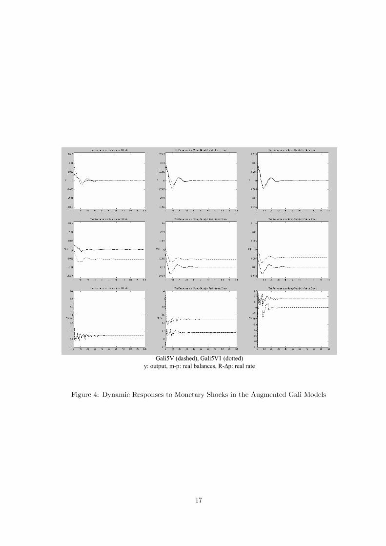
Gali5V (dashed), Gali5V1 (dotted)

y: output, m-p: real balances, R-∆p: real rate

Figure 4: Dynamic Responses to Monetary Shocks in the Augmented Gali Models

17

Table 4: Correlation among the Identified Structural Shocks of KPSW6V, Gali5V and Gali5V1

Model Gali5V,tech Gali5V,ls Gali5V,money Gali5V,ri Gali5V,inf

KPSW6V,bg 0.06 0.62 0.37 0.33 0.16

KPSW6V,inf -0.29 0.11 0.14 -0.31 0.68

KPSW6V,ri 0.15 -0.12 -0.55 0.55 0.44

Model Gali5V1,tech Gali5V1,ls Gali5V1,ri Gali5V1,inf

KPSW6V,bg 0.35 0.71 0.02 -0.03

KPSW6V,inf -0.09 0.21 -0.46 0.63

KPSW6V,ri 0.19 -0.11 0.69 0.56

Notes: Correlation among the identified structural shocks of KPSW6V, Gali5V and Gali5V1. bg: balanced-growth.

tech: technology. inf: inflation. ls: labor supply. ri: real interest.

The correlation coefficients reported in Table 4 support our interpretation regarding the real-

balances, real-interest and inflation shocks. The coefficients of the shocks lie between 0.46 and 0.69

in absolute value. The balanced-growth shock of KPSW6V is weakly correlated with the technology

shocks of Gali5V and Gali5V1, but with the labor supply shocks of these models29.

4 Modifying the Basic Models

This section is devoted to the modification of the basic models considered above. We have two

types of investigations in our mind. The first is to check if adding the labor input to both KPSW

models decreases the bias in these models when identifying the technology shocks. The second

is to examine the effects of having two exogenous variables in the VARs, namely oil price and

national defense spending. Adding these variables to the VAR should provide us a more refined

decomposition of the nontechnology shocks.

29Similarly, Alexius and Carlsson (2005) report a high correlation between the technology shock of KPSW3V and

the labor supply shock of Shapiro and Watson (1988).

18

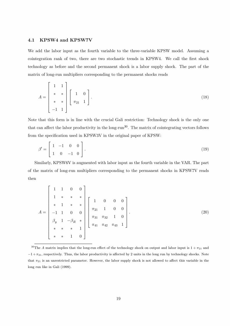
4.1 KPSW4 and KPSW7V

We add the labor input as the fourth variable to the three-variable KPSW model. Assuming a

cointegration rank of two, there are two stochastic trends in KPSW4. We call the first shock

technology as before and the second permanent shock is a labor supply shock. The part of the

matrix of long-run multipliers corresponding to the permanent shocks reads

A =

1 1

∗ ∗∗ ∗−1 1

1 0

π21 1

. (18)

Note that this form is in line with the crucial Gali restriction: Technology shock is the only one

that can affect the labor productivity in the long-run30. The matrix of cointegrating vectors follows

from the specification used in KPSW3V in the original paper of KPSW:

β0 =

1 −1 0 0

1 0 −1 0

. (19)

Similarly, KPSW6V is augmented with labor input as the fourth variable in the VAR. The part

of the matrix of long-run multipliers corresponding to the permanent shocks in KPSW7V reads

then

A =

1 1 0 0

1 ∗ ∗ ∗∗ 1 ∗ ∗−1 1 0 0

βy 1 −βR ∗∗ ∗ ∗ 1

∗ ∗ 1 0

1 0 0 0

π21 1 0 0

π31 π32 1 0

π41 π42 π43 1

. (20)

30The A matrix implies that the long-run effect of the technology shock on output and labor input is 1 + π21 and

−1+π21, respectively. Thus, the labor productivity is affected by 2 units in the long run by technology shocks. Note

that π21 is an unrestricted parameter. However, the labor supply shock is not allowed to affect this variable in the

long run like in Gali (1999).

19

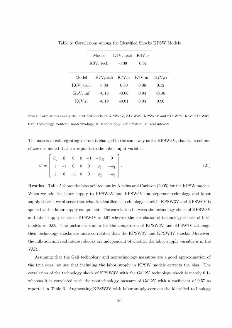
Table 5: Correlations among the Identified Shocks KPSW Models

Model K4V, tech K4V,ls

K3V, tech -0.09 0.97

Model K7V,tech K7V,ls K7V,inf K7V,ri

K6V, tech 0.38 0.80 0.06 0.12

K6V, inf -0.13 -0.06 0.94 -0.06

K6V,ri -0.19 -0.01 0.04 0.96

Notes: Correlations among the identified shocks of KPSW3V, KPSW4V, KPSW6V and KPSW7V. K3V: KPSW3V.

tech: technology. nontech: nontechnology. ls: labor supply. inf: inflation. ri: real interest.

The matrix of cointegrating vectors is changed in the same way as for KPSW3V, that is, a column

of zeros is added that corresponds to the labor input variable:

β0 =

βy 0 0 0 −1 −βR 0

1 −1 0 0 0 φ1 −φ11 0 −1 0 0 φ2 −φ2

. (21)

Results Table 5 shows the bias pointed out by Alexius and Carlsson (2005) for the KPSWmodels.

When we add the labor supply to KPSW3V and KPSW6V and seperate technology and labor

supply shocks, we observe that what is identified as technology shock in KPSW3V and KPSW6V is

spoiled with a labor supply component. The correlation between the technology shock of KPSW3V

and labor supply shock of KPSW4V is 0.97 whereas the correlation of technology shocks of both

models is -0.09. The picture is similar for the comparison of KPSW6V and KPSW7V although

their technology shocks are more correlated than the KPSW3V and KPSW4V shocks. Moreover,

the inflation and real interest shocks are independent of whether the labor supply variable is in the

VAR.

Assuming that the Gali technology and nontechnology measures are a good approximation of

the true ones, we see that including the labor supply in KPSW models corrects the bias. The

correlation of the technology shock of KPSW3V with the Gali2V technology shock is merely 0.14

whereas it is correlated with the nontechnology measure of Gali2V with a coefficient of 0.57 as

reported in Table 6. Augmenting KPSW3V with labor supply corrects the identified technology

20

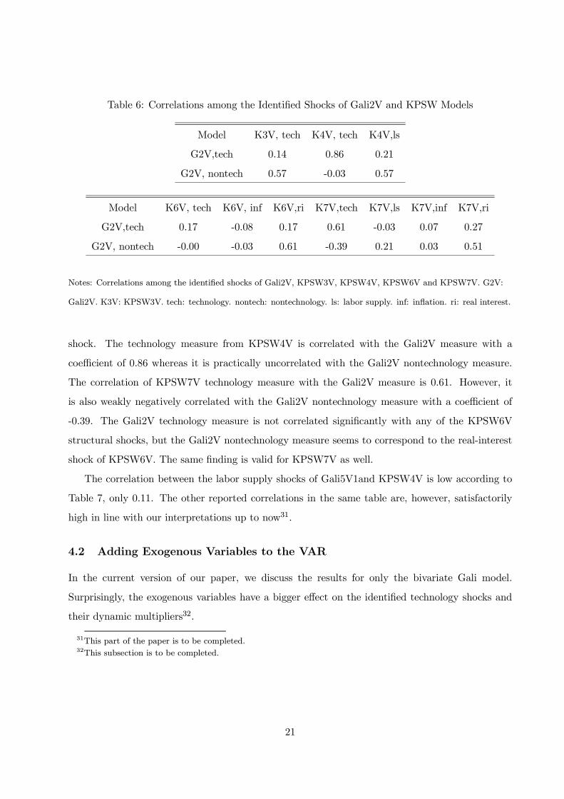
Table 6: Correlations among the Identified Shocks of Gali2V and KPSW Models

Model K3V, tech K4V, tech K4V,ls

G2V,tech 0.14 0.86 0.21

G2V, nontech 0.57 -0.03 0.57

Model K6V, tech K6V, inf K6V,ri K7V,tech K7V,ls K7V,inf K7V,ri

G2V,tech 0.17 -0.08 0.17 0.61 -0.03 0.07 0.27

G2V, nontech -0.00 -0.03 0.61 -0.39 0.21 0.03 0.51

Notes: Correlations among the identified shocks of Gali2V, KPSW3V, KPSW4V, KPSW6V and KPSW7V. G2V:

Gali2V. K3V: KPSW3V. tech: technology. nontech: nontechnology. ls: labor supply. inf: inflation. ri: real interest.

shock. The technology measure from KPSW4V is correlated with the Gali2V measure with a

coefficient of 0.86 whereas it is practically uncorrelated with the Gali2V nontechnology measure.

The correlation of KPSW7V technology measure with the Gali2V measure is 0.61. However, it

is also weakly negatively correlated with the Gali2V nontechnology measure with a coefficient of

-0.39. The Gali2V technology measure is not correlated significantly with any of the KPSW6V

structural shocks, but the Gali2V nontechnology measure seems to correspond to the real-interest

shock of KPSW6V. The same finding is valid for KPSW7V as well.

The correlation between the labor supply shocks of Gali5V1and KPSW4V is low according to

Table 7, only 0.11. The other reported correlations in the same table are, however, satisfactorily

high in line with our interpretations up to now31.

4.2 Adding Exogenous Variables to the VAR

In the current version of our paper, we discuss the results for only the bivariate Gali model.

Surprisingly, the exogenous variables have a bigger effect on the identified technology shocks and

their dynamic multipliers32.

31This part of the paper is to be completed.32This subsection is to be completed.

21

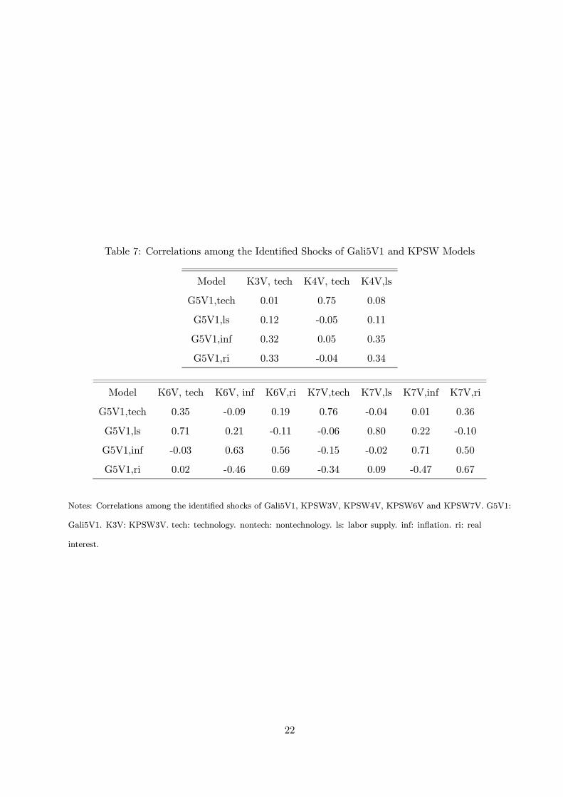
Table 7: Correlations among the Identified Shocks of Gali5V1 and KPSW Models

Model K3V, tech K4V, tech K4V,ls

G5V1,tech 0.01 0.75 0.08

G5V1,ls 0.12 -0.05 0.11

G5V1,inf 0.32 0.05 0.35

G5V1,ri 0.33 -0.04 0.34

Model K6V, tech K6V, inf K6V,ri K7V,tech K7V,ls K7V,inf K7V,ri

G5V1,tech 0.35 -0.09 0.19 0.76 -0.04 0.01 0.36

G5V1,ls 0.71 0.21 -0.11 -0.06 0.80 0.22 -0.10

G5V1,inf -0.03 0.63 0.56 -0.15 -0.02 0.71 0.50

G5V1,ri 0.02 -0.46 0.69 -0.34 0.09 -0.47 0.67

Notes: Correlations among the identified shocks of Gali5V1, KPSW3V, KPSW4V, KPSW6V and KPSW7V. G5V1:

Gali5V1. K3V: KPSW3V. tech: technology. nontech: nontechnology. ls: labor supply. inf: inflation. ri: real

interest.

22

5 Which Shocks Explain the Fluctuations of the Variables?

Forecast-error variance decomposition (FEVD) is a tool that is widely used in the SVAR literature

in order to find out which structural shocks explain the fluctuations of macroeconomic variables

in different horizons, typically business cycle horizons. A traditional definition of business cycle

horizon is from six to thirty two quarters. Because of this long span of time, it is possible that a

researcher may come to inconclusive results regarding the source of fluctuations. One example can

be found in KPSW. The authors report in Table 5 of their paper that the fraction of the forecast-

error variance attributable to real-interest-rate shock of output is 74 percent in four quarters,

55 percent in eight quarters and 25 percent in twenty four quarters. On the other hand, the

contribution of balanced-growth (technology) shock on output is 5 percent in four quarters, 22

percent in eight quarters and 62 percent in twenty four quarters. Hence, it is not possible to detect

if one of these shocks is more important for the fluctuations.

We propose in the following to consider the whole business cycle horizon when computing error

variance decompositions. Our approach resembles the one used by Crucini (2006), see Equation

(2.5) in his paper. The error variance decomposition of variable xi is computed by employing the

relationship

std(xi) =Xj

std (xi,j) · corr (xi,j, xi) . (22)

To be precise, xi stands in this paper for the business cycle component of the original variable

computed using the HP filter. xi,j is the historical component of xi w.r.t. the jth structural shock

in the VAR. std(xi) is the standard deviation of xi and corr (xi,j , xi) is the correlation between xi,j

and xi. Then,std(xi,j)·corr(xi,j ,xi)

std(xi)gives the contribution of the jth structural shock to the business

cycle fluctuations of xi. Notice that this type of a decomposition allows us to see if the propagation

mechanism or the volatility of a certain shock explains the fluctuations of a variable more. For

example, it is possible that the business cycle component of a variable is highly correlated with all

of its historical components. In this case, the shock which is more volatile than the others plays

obviously a bigger role in the business cycle fluctuations of the variable. We can also turn this

picture upside down: It is not to discard that a structural shock plays a big role as it has a large

volatility, although the historical component that corresponds to it is not so highly correlated with

the original variable.

In the following xdi represents the cyclical component of the original time series computed using

the HP-filter. The superscript d stands for “data”. Furthermore, we define xmi =Pj xij where the

23

superscript m stands for “model”. In case all the shocks in the VAR are computed, regardless of

whether they are all given an economic interpretation, xdi ≈ xmi holds. This is indeed an almost

exact relationship. Recall that we can compute all the shocks and the corresponding historical

components of the variables in the BQ identification scheme, but not in the KPSW scheme. Thus,

the KPSW scheme implies xdi 6= xmi =Pj 6=k xij with k being the index of transitory shocks. It

follows thatxmixdi≈ 1 when the BQ scheme is applied. The ratio

xmixdiindicates but the total share

of the permanent shocks in the business cycle fluctuations of xi if KPSW scheme is employed. For

both BQ and KPSW schemes, we can write

std(xdi ) =Xj

std (xi,j) · corr (xi,j, xmi ) + ε (23)

where ε is an error term. Within the BQ framework, (23) is expected to hold with ε ≈ 0. For

example, the correlation and the relative standard deviation of output, ym and yd, are 1 and

0.98 in the bivariate Gali model, respectively. Moreover, the share of all the shocks,Pj std (yj) ·

corr (yj, ym) /std(yd), obtains 0.98, see Table 8. ε refers to the approximation error plus the share of

the transitory shocks in the KPSW framework. Recall that std(xmi ) =Pj 6=k std (xi,j)·corr (xi,j , xmi )

with k being the index for transitory shocks is an exact relationship. Therefore, we compute the

share of the jth shock as

std (xi,j) · corr (xi,j , xmi )std(xdi )

. (24)

in this paper.

The above proposed error variance decomposition reestablishes the results in Gali (1999). Non-

technology shocks are the main driving force of business cycle fluctuations in output and labor input

according to the bivariate model as reported in Table 8. The nontechnology share amounts to 0.87

and 0.89 for output and labor input, respectively. However, technology and nontechnology shocks

have a balanced weight in the fluctuations of labor productivity, the share of technology shocks

being 0.45 and nontechnology shocks 0.52. The five-variable Gali model with cointegration leads

to similar findings. The share of technology shocks in output, labor input and labor productivity is

0.08, 0.14 and 0.32, respectively, not much different from their values in the bivariate model, 0.10,

0.10 and 0.45.

According to Gali5V1, the labor supply shocks have the biggest share in the fluctuations of

real balances with 0.56 whereas the total share of real interest and inflation shock is merely 0.30.

Furthermore, the total share of supply, i.e. technology plus labor supply, shocks in real balances is

24

Table 8: Shares of Structural Shocks in the Business Cycle Components of the Variables in Gali2V

tech nontech sum

y 0.10 0.87 0.98

n 0.10 0.89 0.98

x 0.45 0.52 0.97

Notes: The correlation between a variable and its components w.r.t technology and nontechnology shocks. tech:

technology. nontech: nontechnology.

0.71 which is perhaps against the general intuition. We find this result puzzling and believe that it

should be investigated further in new of versions of this paper. We also establish that supply shocks’

total share is 0.45 in the fluctuations of inflation, that is, inflation is a supply side phenomena as

much as a demand side phenomena according to Gali5V1.

Gali5V1 is a model with four permanent shocks and only one transitory shock. Therefore, we

see that the total share of the permanent shocks is close to one for the variables of the model.

KPSW7V, with four permanent and three transitory shocks, attributes, on the other hand, shares

of 0.72 - 0.82 to permanent shocks as reported in Table 9. The real interest shock has the largest

share with 0.47 in the fluctuations of output whereas the total share of technology and labor supply

shocks is 0.21. The puzzle mentioned above concerning the fluctuations of real balances exists in

KPSW7V, too. Supply shocks explain its variability much more (with a share of 0.53) than the

demand (monetary) shocks (with a share of 0.27). Not like in Gali5V1, the inflation fluctuations

are more the result of real interest and inflation shocks in KPSW7V.

6 Conclusion

According to Blanchard and Quah (1993), the entire point of structural VAR analysis is exactly

identification of alternative disturbances. Thus, all possibilities need to be considered. Although we

cannot claim to have considered all possibilities in this paper yet, we attempted to consider some

more possibilities than suggested up to now in the related literature.

An SVAR model alone cannot be helpful or reliable as an empirical method. It is necessary to

check the ability of an SVAR to capture the phenomenon that it is supposed to capture using other

methods than SVAR. Once this ability is established, SVARs can be used to recover the general

25

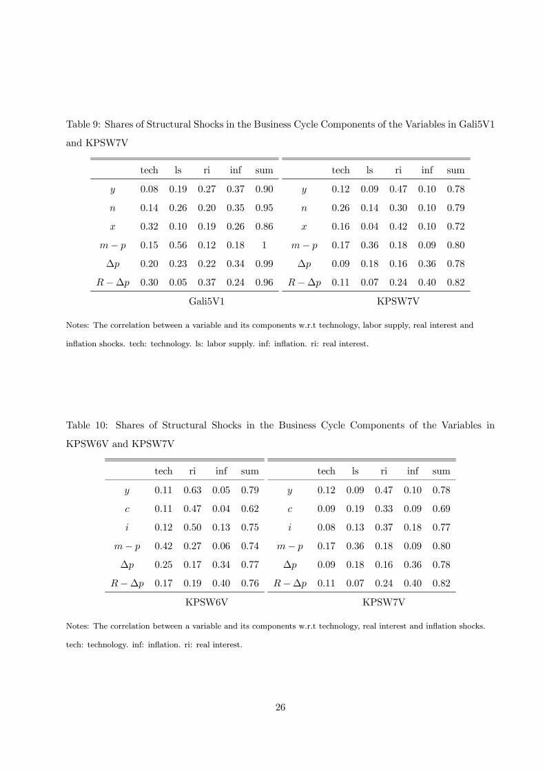
Table 9: Shares of Structural Shocks in the Business Cycle Components of the Variables in Gali5V1

and KPSW7V

tech ls ri inf sum

y 0.08 0.19 0.27 0.37 0.90

n 0.14 0.26 0.20 0.35 0.95

x 0.32 0.10 0.19 0.26 0.86

m− p 0.15 0.56 0.12 0.18 1

∆p 0.20 0.23 0.22 0.34 0.99

R−∆p 0.30 0.05 0.37 0.24 0.96

Gali5V1

tech ls ri inf sum

y 0.12 0.09 0.47 0.10 0.78

n 0.26 0.14 0.30 0.10 0.79

x 0.16 0.04 0.42 0.10 0.72

m− p 0.17 0.36 0.18 0.09 0.80

∆p 0.09 0.18 0.16 0.36 0.78

R−∆p 0.11 0.07 0.24 0.40 0.82

KPSW7V

Notes: The correlation between a variable and its components w.r.t technology, labor supply, real interest and

inflation shocks. tech: technology. ls: labor supply. inf: inflation. ri: real interest.

Table 10: Shares of Structural Shocks in the Business Cycle Components of the Variables in

KPSW6V and KPSW7V

tech ri inf sum

y 0.11 0.63 0.05 0.79

c 0.11 0.47 0.04 0.62

i 0.12 0.50 0.13 0.75

m− p 0.42 0.27 0.06 0.74

∆p 0.25 0.17 0.34 0.77

R−∆p 0.17 0.19 0.40 0.76

KPSW6V

tech ls ri inf sum

y 0.12 0.09 0.47 0.10 0.78

c 0.09 0.19 0.33 0.09 0.69

i 0.08 0.13 0.37 0.18 0.77

m− p 0.17 0.36 0.18 0.09 0.80

∆p 0.09 0.18 0.16 0.36 0.78

R−∆p 0.11 0.07 0.24 0.40 0.82

KPSW7V

Notes: The correlation between a variable and its components w.r.t technology, real interest and inflation shocks.

tech: technology. inf: inflation. ri: real interest.

26

tendencies and structures in economic data. In this sense, macroeconomic theories can be judged

with the help of SVAR models.

Nontechnology shocks are the main driving force behind the business cycle fluctuations. In

particular, shocks to nominal/monetary variables are found to be important in the fluctuations of

real variables like output, consumption and investment.

27

References

Alexius, A. and M. Carlsson, 2005, “Measures of Technology and the Business Cycle”, TheReview of Economics and Statistics, 87(2), 299-307

Alexius, A. andM. Carlsson, 2001, “Measures of Technology and the Business Cycle: Evidencefrom Sweden and the U.S.”, FIEF Working Paper Series, No. 174

Basu, S. and M.S. Kimball, 1997, “Cyclical Productivity with Unobserved Input Variation”,NBER Working Paper, No. 5915

Blanchard, O.J. and D. Quah, 1989, “The Dynamic Effects of Aggregate Demand and SupplyDisturbances”, The American Economic Review, Vol.79, No. 4, 655-673

Blanchard, O.J. and D. Quah, 1993, “The Dynamic Effects of Aggregate Demand and SupplyDisturbances: Reply”, The American Economic Review, Vol. 83, No. 3, 653-658

Breitung, Jorg, 2000, “Structural Inference in Cointegrated Vector Autoregressive Models”,Habilitation Thesis, Humboldt University Berlin

Christiano L.J., Eichenbaum, M. and C.L. Evans, 1999, “Monetary Policy Shocks: WhatHave We Learned and to What End?” in Handbook of Macroeconomics, M. Woodford and J.Taylor, eds., Vol. 1A, Amsterdam: North Holland

Faust, J. and E. Leeper, 1997, “When Do Long-Run Identifying Restrictions Give ReliableResults”, Journal of Business and Economic Statistics, 15, 345-353

Gali, J., 1999, “Technology, Employment and the Business Cycle: Do Technology ShocksExplain Aggregate Fluctuations?”, The American Economic Review, Vol. 89, No. 1, 249-271

Gali, J. and P. Rabanal, 2004, “Technology Shocks and Aggregate Fluctuations: HowWell Does the Real Business Cycle Model Fit Postwar U.S. Data?”, IMF Working Paper,WP/04/234

Jang, K. and M. Ogaki, 2001, “User Guide for VECM with Long-Run Restrictions”, TheOhio State University, Manuscript

King, R., Plosser, C., Stock, J. and M. Watson, 1991, “Stochastic Trends and EconomicFluctuations”, The American Economic Review, Vol. 81, No. 4, 819-840

Lutkepohl, H., 2006, New Introduction to Multiple Time Series Analysis, Springer, Berlin

Shapiro, M.D. and M. Watson (1988), “Sources of Business Cycle Fluctuations”, CowlesFoundation Discussion Paper, No. 870

28