a comparison of peripheral imaging technologies for bone ... · a comparison of peripheral imaging...

265

J Musculoskelet Neuronal Interact 2016; 16(4):265-282

Review Article

A comparison of peripheral imaging technologies for bone and muscle quantification: a technical review of image acquisition

A.K.O. Wong1,2

1Joint Department of Medical Imaging, Toronto General Research Institute, University Health Network, Toronto, ON, Canada; 2McMaster University, Department of Medicine, Faculty of Health Sciences, Hamilton, ON, Canada

Introduction

Our understanding of fracture risk has evolved from exam-ining areal bone mineral density (aBMD) from dual energy X-ray absorptiometry (DXA), to other risk factors for fractures in tools like FRAX1. It is clear that we need to understand fac-tors beyond aBMD to gauge a clearer picture of an individu-al’s fracture risk2. While DXA can provide lean mass, fat mass, and bone mass information, its two-dimensional scans fail to enable separation of cortical from trabecular bone, skeletal muscle from other lean organs, and its measurements and precision are sensitive to body size3 due to significant soft tissue contribution to the attenuation of X-rays4. Peripheral

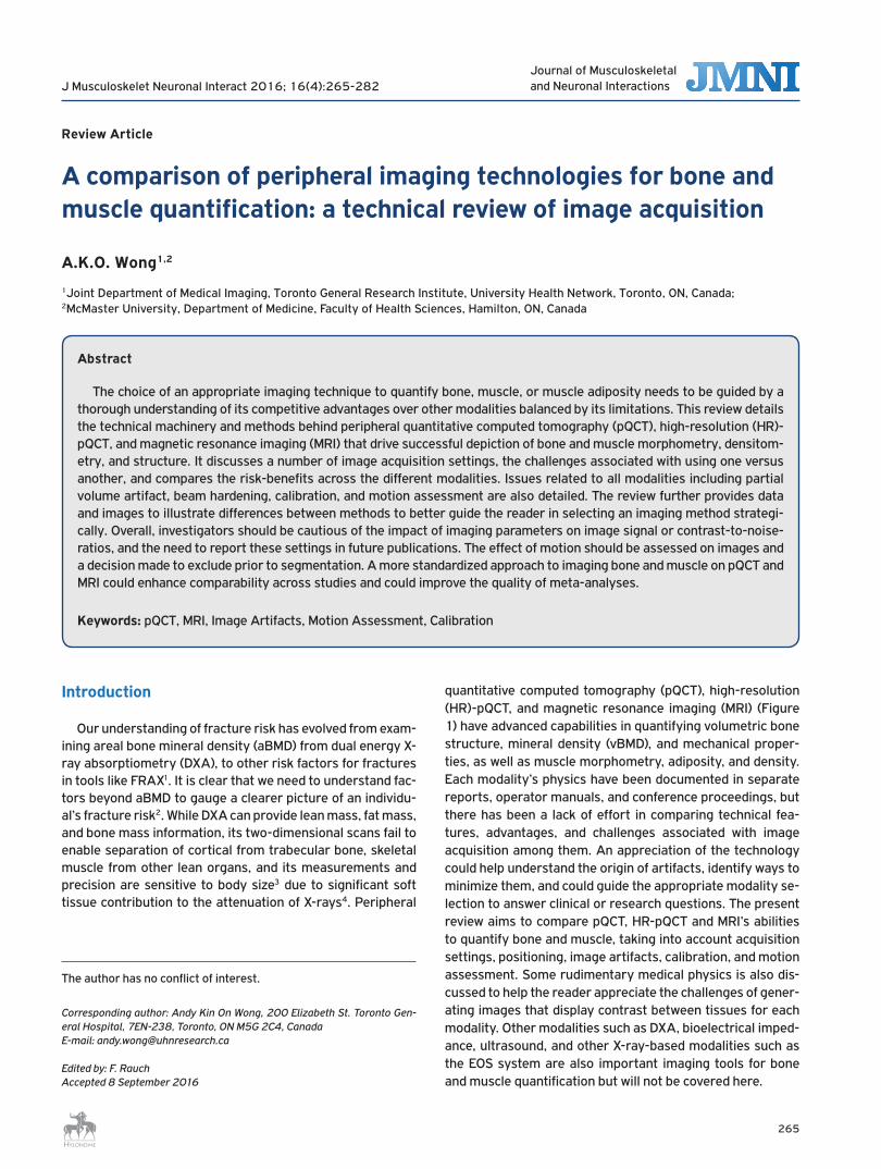
quantitative computed tomography (pQCT), high-resolution (HR)-pQCT, and magnetic resonance imaging (MRI) (Figure 1) have advanced capabilities in quantifying volumetric bone structure, mineral density (vBMD), and mechanical proper-ties, as well as muscle morphometry, adiposity, and density. Each modality’s physics have been documented in separate reports, operator manuals, and conference proceedings, but there has been a lack of effort in comparing technical fea-tures, advantages, and challenges associated with image acquisition among them. An appreciation of the technology could help understand the origin of artifacts, identify ways to minimize them, and could guide the appropriate modality se-lection to answer clinical or research questions. The present review aims to compare pQCT, HR-pQCT and MRI’s abilities to quantify bone and muscle, taking into account acquisition settings, positioning, image artifacts, calibration, and motion assessment. Some rudimentary medical physics is also dis-cussed to help the reader appreciate the challenges of gener-ating images that display contrast between tissues for each modality. Other modalities such as DXA, bioelectrical imped-ance, ultrasound, and other X-ray-based modalities such as the EOS system are also important imaging tools for bone and muscle quantification but will not be covered here.

Abstract

The choice of an appropriate imaging technique to quantify bone, muscle, or muscle adiposity needs to be guided by a thorough understanding of its competitive advantages over other modalities balanced by its limitations. This review details the technical machinery and methods behind peripheral quantitative computed tomography (pQCT), high-resolution (HR)-pQCT, and magnetic resonance imaging (MRI) that drive successful depiction of bone and muscle morphometry, densitom-etry, and structure. It discusses a number of image acquisition settings, the challenges associated with using one versus another, and compares the risk-benefits across the different modalities. Issues related to all modalities including partial volume artifact, beam hardening, calibration, and motion assessment are also detailed. The review further provides data and images to illustrate differences between methods to better guide the reader in selecting an imaging method strategi-cally. Overall, investigators should be cautious of the impact of imaging parameters on image signal or contrast-to-noise-ratios, and the need to report these settings in future publications. The effect of motion should be assessed on images and a decision made to exclude prior to segmentation. A more standardized approach to imaging bone and muscle on pQCT and MRI could enhance comparability across studies and could improve the quality of meta-analyses.

Keywords: pQCT, MRI, Image Artifacts, Motion Assessment, Calibration

The author has no conflict of interest.

Corresponding author: Andy Kin On Wong, 200 Elizabeth St. Toronto Gen-eral Hospital, 7EN-238, Toronto, ON M5G 2C4, CanadaE-mail: [email protected]

Edited by: F. RauchAccepted 8 September 2016

Journal of Musculoskeletaland Neuronal Interactions

266http://www.ismni.org

A.K.O. Wong: Comparing technologies for musculoskeletal imaging

Overview of CT

The International Society for Clinical Densitometry (ISCD) published its first recommendations in 2008 on evidence for the use of QCT and pQCT technologies in managing osteo-porosis in adults5; and within the same year, issued recom-mendations on the need for establishing reference data and for standardizing bone measurements on pQCT for children and adolescents6. To better appreciate how QCT collects in-formation on bones and soft tissue properties, a brief discus-sion of its medical physics will be useful. QCT operates on the physics of photoelectric absorption. The amount of photons passing through a material can be represented by the Beer-Lambert law (Equation 1), which indicates that the intensity of transmitted (I

out) versus the intensity of incident (I

in) pho-

tons is negatively related to the object thickness (d), and the linear attenuation coefficient (µ), which is governed by pho-ton energy, and object density:

Iout

Iin= -e

µχd Equation 1. Beer-Lambert Law.

The thicker and denser the object examined, the fewer photons will be captured by detectors. With bone being able to attenuate more photons than muscle, followed by fat, dif-ferences in linear attenuation of these tissues allow QCT to separately quantify structural features. pQCT and HR-pQCT can yield vBMD and structural information at the distal radius and tibia. pQCT first led muscle analyses at more proximal scan locations7. HR-pQCT only more recently explored soft tissue analysis using distal tibia scans8 and is now developing

the technique at more proximal sites on its second genera-tion machines (Kapadia R., personal communication). Each of these modalities was developed by different manufacturers. The first type of pQCT, the Densiscan-1000 by Scanco Medi-cal AG (Bruettisellen, Switzerland) was distributed in 1988. The pQCT as we know it today was later manufactured in 1992 by Stratec Medizintechnik (Pforzheim, Germany) who has since established the XCT900, XCT960, XCT2000 (col-limation enabled), XCT2000L (longer z-axis than XCT2000), and XCT3000 (larger gantry than XCT2000). The HR-pQCT was first distributed in 2004 by Scanco Medical AG (Bru-ettisellen, Switzerland), branded as the XtremeCT and by mid-2014 began marketing XtremeCT II (larger stack, faster scanning, smaller voxel size, deeper z-axis).

pQCT technology & acquisition settings

pQCT is a sequential QCT designed for compactness and portability while specializing in bone and muscle quantifica-tion9. The technology uses cadmium telluride (CdTe) detec-tors that operate over a range of temperatures with little concern over leakage current. Although energy resolution for CdTe is poorer than silicon detectors, smaller pixel sizes are enabled by separating crystals apart by 1o (Rawer, R., Stratec, personal communication). The 12 detectors integrate image data across 180 projections into tomographic slices by fil-tered back-projection against a 256 x 256 pixel matrix9. Scan speeds range from 10 to 50 mm/s. The smallest voxel size

Figure 1. Illustration of different peripheral QCT and MRI technologies. A) Scanco Densiscan 1000 (pQCT), B) Scanco Medical Xtrem-eCT1/2 (HR-pQCT), C) Stratec Medizintechnik XCT2000 (pQCT), D) Stratec Medizintechnik XCT3000 (pQCT), E) General Electric ONI MSK Extreme 1.0T (pMRI), F) Esaote SpA O-Scan 0.31T (pMRI), G) General Electric Lunar Artoscan M Extremity 0.2T MRI, H) General Electric MagneVu MV1000 0.2T MRI. Only B to F are currently available.



achievable with XCT2000 and beyond is 200 µm (range 200-800 µm in-plane) using a source and detector collimator (4 x 0.8 mm aperture per detector). Scans operate at an X-ray voltage of 58-60 kV, a spot size of 50 µm, and a fan-beam geometry9. Because the back of the scanner is open, there is an unlimited gantry depth. However, the maximum object length is 400 mm, based on the maximum travel z-distance. Depending on the scanner generation, maximum object diam-eter can be 140 mm (XCT2000) or 270 mm (XCT3000), the latter being able to accommodate knees and thighs. Standard slice thickness remains at 2.0±0.5 mm in either case. Ionizing radiation is but a minor concern for pQCT scans with an effec-tive dose of 1 µSv per tomographic slice. As a reference, the

Canadian Nuclear Safety Commission established a dose limit of 1000 µSv for the general public per calendar year above background radiation, which has been reported to be 1800 µSv averaged across 16 cities in Canada10.

pQCT differences in scan speed and in-plane pixel size

pQCT scan protocols have not been standardized. A sur-vey of previous studies using pQCT employed a range of scan speeds (10,15,20,25 mm/s) and in-plane pixel sizes (0.200,0.300,0.400,0.500 mm) (Table 1). Acquisition of scans at a slower speed enables longer integration time, during which more image data could be back-projected to

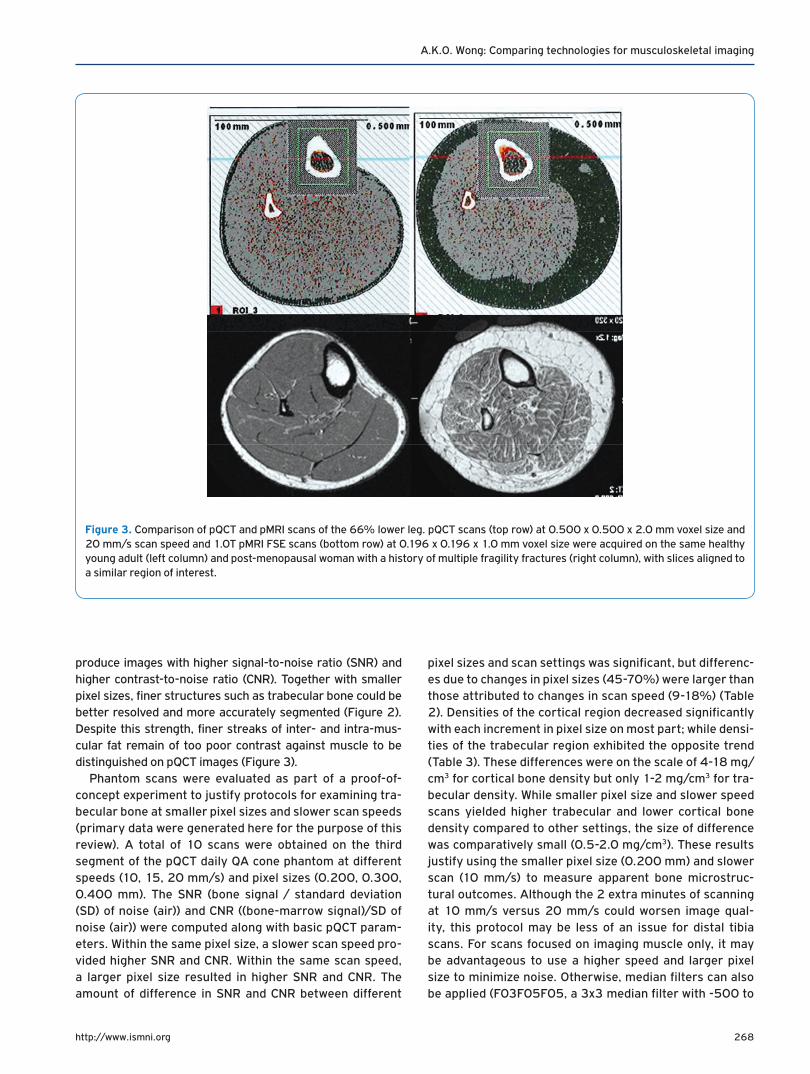
Table 1. Survey of studies employing different in-plane pixel sizes and scan speeds. Macro = macrostructural bone parameters (vBMD, Ct.Th, total and cross-sectional area, SSIp), Micro = microstructural bone parameters (BV/TV, Tb.Sp, Tb.Th, Tb.N).

Authors & YearScan Speed

(mm/s)Resolution (mm) % Sites examined

Bone reported

Muscle reported

(11) Rauch & Schoenau 2005 15 0.400 4% Rad Macro No

(12) Fung et al, 2011 25 0.400 3% Tib, 66% Tib Macro Yes

(13) Mantila Roosa et al, 2012 20 0.300 80% Hum Macro No

(14) Eser et al, 2010 15 0.300 4,50% MCP Macro Yes

(15) Sheu et al, 2011 20 0.5004,33% Rad

4,33,66% TibMacro No

(16) Weidauer et al, 2014 20 0.500 4,20,66% Tib Macro Yes

(17) Kontulainen et al, 2007 10 0.200 25% Tib (Ex Vivo) Macro No

(18) Wong et al, 2014 10 0.200 4% Rad & TibMicro & Macro

No

Rad = radius, Tib = tibia, Hum = humerus, MCP = metacarpal; vBMD = volumetric bone mineral density; Ct.Th = cortical thickness; SSIp= polar strength-strain index; BV/TV = bone volume to total volume; Tb.Sp = trabecular separation; Tb.Th = trabecular thickness; Tb.N= trabecular number.

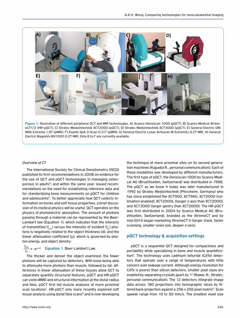
Figure 2. Comparison of image quality and noise among varying scan speeds and in-plane pixel sizes. Slower scans and smaller in-plane pixel sizes result in more background noise but clearer contrast between fine structures.



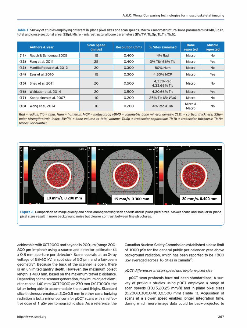
produce images with higher signal-to-noise ratio (SNR) and higher contrast-to-noise ratio (CNR). Together with smaller pixel sizes, finer structures such as trabecular bone could be better resolved and more accurately segmented (Figure 2). Despite this strength, finer streaks of inter- and intra-mus-cular fat remain of too poor contrast against muscle to be distinguished on pQCT images (Figure 3).

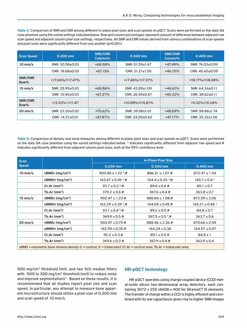
Phantom scans were evaluated as part of a proof-of-concept experiment to justify protocols for examining tra-becular bone at smaller pixel sizes and slower scan speeds (primary data were generated here for the purpose of this review). A total of 10 scans were obtained on the third segment of the pQCT daily QA cone phantom at different speeds (10, 15, 20 mm/s) and pixel sizes (0.200, 0.300, 0.400 mm). The SNR (bone signal / standard deviation (SD) of noise (air)) and CNR ((bone-marrow signal)/SD of noise (air)) were computed along with basic pQCT param-eters. Within the same pixel size, a slower scan speed pro-vided higher SNR and CNR. Within the same scan speed, a larger pixel size resulted in higher SNR and CNR. The amount of difference in SNR and CNR between different

pixel sizes and scan settings was significant, but differenc-es due to changes in pixel sizes (45-70%) were larger than those attributed to changes in scan speed (9-18%) (Table 2). Densities of the cortical region decreased significantly with each increment in pixel size on most part; while densi-ties of the trabecular region exhibited the opposite trend (Table 3). These differences were on the scale of 4-18 mg/cm3 for cortical bone density but only 1-2 mg/cm3 for tra-becular density. While smaller pixel size and slower speed scans yielded higher trabecular and lower cortical bone density compared to other settings, the size of difference was comparatively small (0.5-2.0 mg/cm3). These results justify using the smaller pixel size (0.200 mm) and slower scan (10 mm/s) to measure apparent bone microstruc-tural outcomes. Although the 2 extra minutes of scanning at 10 mm/s versus 20 mm/s could worsen image qual-ity, this protocol may be less of an issue for distal tibia scans. For scans focused on imaging muscle only, it may be advantageous to use a higher speed and larger pixel size to minimize noise. Otherwise, median filters can also be applied (F03F05F05, a 3x3 median filter with -500 to

Figure 3. Comparison of pQCT and pMRI scans of the 66% lower leg. pQCT scans (top row) at 0.500 x 0.500 x 2.0 mm voxel size and 20 mm/s scan speed and 1.0T pMRI FSE scans (bottom row) at 0.196 x 0.196 x 1.0 mm voxel size were acquired on the same healthy young adult (left column) and post-menopausal woman with a history of multiple fragility fractures (right column), with slices aligned to a similar region of interest.



500 mg/cm3 threshold limit, and two 5x5 median filters with -500 to 300 mg/cm3 threshold limit) to reduce noise and improve segmentations11. Based on these results, it is recommended that all studies report pixel size and scan speed. In particular, any attempt to measure bone appar-ent microstructure should utilize a pixel size of 0.200 mm and scan speed of 10 mm/s.

HR-pQCT technology

HR-pQCT operates using charge coupled device (CCD) met-al-oxide silicon two-dimensional array detectors, each con-taining 3072 x 255 (4608 x 400 for XtremeCT II) elements. The transfer of charge within a CCD is highly efficient and com-bined with its low capacitance gives rise to higher SNR images

Table 2. Comparison of SNR and CNR among different in-plane pixel sizes and scan speeds on pQCT. Scans were performed on the daily QA cone phantom using the varied settings indicated below. Row and column percentages represent amount of difference between adjacent row scan speed and adjacent column pixel size settings, respectively. All SNR and CNR values derived from various combinations of scan speeds and pixel sizes were significantly different from one another (p<0.001).

Scan Speed 0.200 mmSNR/CNRColumn%

0.300 mmSNR/CNRColumn%

0.400 mm

10 mm/s SNR: 30.58±0.03 +68.58% SNR: 51.55±1.67 +47.49% SNR: 76.03±0.09

CNR: 18.68±0.03 +67.13% CNR: 31.21±1.00 +46.10% CNR: 45.60±0.09

SNR/CNRRow%

+17.66%/+17.47% +17.46%/+17.37% +18.17%/+18.08%

15 mm/s SNR: 25.99±0.03 +68.86% SNR: 43.89±1.09 +46.61% SNR: 64.34±0.11

CNR: 15.90±0.03 +67.27% CNR: 26.59±0.67 +45.22% CNR: 38.62±0.11

SNR/CNR Row%

+12.03% /+11.87 +10.88%/+10.81% +9.32%/+9.34%

20 mm/s SNR: 23.20±0.02 +70.62% SNR: 39.58±1.01 +48.69% SNR: 58.86±1.74

CNR: 14.21±0.01 +67.87% CNR: 24.00±0.62 +47.17% CNR: 35.32±1.06

Table 3. Comparison of density and areal measures among different in-plane pixel sizes and scan speeds on pQCT. Scans were performed on the daily QA cone phantom using the varied settings indicated below. * Indicates significantly different from adjacent row speed and # indicates significantly different from adjacent column pixel sizes, both at the 95% confidence level.

Scan Speed

In-Plane Pixel Size

0.200 mm 0.300 mm 0.400 mm

10 mm/s vBMDc (mg/cm3) 900.48 ± 1.22 *,# 886.21 ± 1.07 # 872.47 ± 1.34

vBMDtr (mg/cm3) 163.67 ± 0.45 *,# 164.4 ± 0.25 *,# 165.7 ± 0.4 *

Ct.Ar (mm2) 93.7 ± 0.3 *,# 89.6 ± 0.6 # 85.1 ± 0.7

Tb.Ar (mm2) 370.2 ± 0.6 # 367.6 ± 0.4 # 363.8 ± 0.7

15 mm/s vBMDc (mg/cm3) 902.47 ± 1.23 # 886.84 ± 1.08 # 872.59 ± 2.06

vBMDtr (mg/cm3) 163.29 ± 0.39 *,# 164.09 ± 0.45 # 165.21 ± 0.46 *

Ct.Ar (mm2) 93.1 ± 0.4 *,# 89.2 ± 0.5 # 84.8 ± 0.7

Tb.Ar (mm2) 369.9 ± 0.5 # 367.5 ± 0.5 *,# 363.7 ± 0.6

20 mm/s vBMDc (mg/cm3) 903.47 ± 0.79 # 888.46 ± 2.36 # 870.66 ± 2.59

vBMDtr (mg/cm3) 162.59 ± 0.35 # 164.24 ± 0.36 164.57 ± 0.47

Ct.Ar (mm2) 92.2 ± 0.3 # 89.1 ± 0.5 # 84.8 ± 1

Tb.Ar (mm2) 369.6 ± 0.3 # 367.9 ± 0.4 # 363.9 ± 0.4

vBMD = volumetric bone mineral density (c = cortical; tr = trabecular); Ct.Ar = cortical area; Tb.Ar = trabecular area.



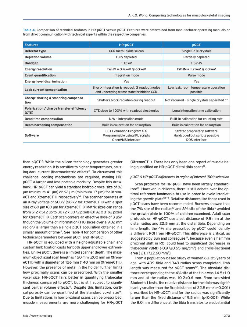
than pQCT12. While the silicon technology generates greater energy resolution, it is sensitive to higher temperatures, caus-ing dark current (thermoelectric effect)13. To circumvent this challenge, cooling mechanisms are required, making HR-pQCT a larger and less portable modality. Despite this draw-back, HR-pQCT can yield a standard isotropic voxel size of 82 µm (minimum 41 µm) or 62 µm (minimum 17 µm) for Xtrem-eCT and XtremeCT II, respectively14. The scanner operates at an X-ray voltage of 60 kV (68 kV for XtremeCT II) with a spot size of 60 µm (80 µm for XtremeCT II). Matrix sizes can range from 512 x 512 up to 3072 x 3072 pixels (8192 x 8192 pixels for XtremeCT II). Each scan confers an effective dose of 3 µSv, though the volume of information (110 slices over a 9.02 mm region) is larger than a single pQCT acquisition obtained in a similar amount of time14. See Table 4 for comparison of other technical parameters between pQCT and HR-pQCT.

HR-pQCT is equipped with a height-adjustable chair and custom limb fixation casts for both upper and lower extremi-ties. Unlike pQCT, there is a limited scanner depth. The maxi-mum object axial scan length is 150 mm (200 mm on Xtrem-eCT II) with a diameter of 126 mm (140 mm on XtremeCT II). However, the presence of metal in the holder further limits how proximally scans can be prescribed. With the smaller voxel size, HR-pQCT fairs better in quantifying trabecular thickness compared to pQCT, but is still subject to signifi-cant partial volume effects15. Despite this limitation, corti-cal porosity can be quantified at the standard voxel size16. Due to limitations in how proximal scans can be prescribed, muscle measurements are more challenging for HR-pQCT

(XtremeCT I). There has only been one report of muscle be-ing quantified on HR-pQCT distal tibia scans8.

pQCT & HR-pQCT differences in region of interest (ROI) selection

Scan protocols for HR-pQCT have been largely standard-ized17. However, in children, there is still debate over the op-timal reference landmarks to use in order to avoid irradiat-ing the growth plate18,19. Relative distances like those used in pQCT scans have been recommended. Burrows showed that the 7% site of the radius20 and 8% site of the tibia19 avoided the growth plate in 100% of children examined. Adult scan protocols on HR-pQCT use a set distance of 9.5 mm at the distal radius and 22.5 mm at the distal tibia. Depending on limb length, the 4% site prescribed by pQCT could identify a different ROI from HR-pQCT. This difference is critical, as suggested by Sun and colleagues21, because even a half mm proximal shift in ROI could lead to significant decreases in trabecular vBMD (-0.97±0.55 mg/cm3) and cross-sectional area (-21.17±2.60 mm2).

From a population-based study of women 60-85 years of age, with 409 tibia and 349 radius scans completed, limb length was measured for pQCT scans22. The absolute dis-tance corresponding to the 4% site at the tibia was 14.5±1.0 mm and at the radius was 10.2±0.6 mm. From two-sided Student’s t tests, the relative distance for the tibia was signif-icantly smaller than the fixed distance of 22.5 mm (p<0.001) prescribed by HR-pQCT; and for the radius was significantly larger than the fixed distance of 9.5 mm (p<0.001). While the 8.0 mm difference at the tibia translates to a substantial

Table 4. Comparison of technical features in HR-pQCT versus pQCT. Features were determined from manufacturer operating manuals or from direct communication with technical experts within the respective companies.

Features HR-pQCT pQCT

Detector type CCD metal-oxide silicon Single CdTe crystals

Depletion volume Fully depleted Partially depleted

Bandgap 1.12 eV 1.52 eV

Energy resolution FWHM = 0.4 keV @ 60 keV FWHM = 1.7 keV @ 60 keV

Event quantification Integration mode Pulse mode

Energy level discrimination Yes Yes

Leak current compensationShort- integration & readout, 3 readout nodes

and underlying frame transfer hidden CCDLow leak, room temperature operation

possible

Charge sharing & smearing compensa-tion

Shutters block radiation during readout Not required – single crystals separated 1o

Polarization / charge transfer efficiency (CTE)

CTE close to 100% with readout electronics Long integration time calibration

Dead time compensation N/A – integration mode Built-in calibration for counting rate

Beam hardening compensation Built-in calibration for absorption Built-in calibration for absorption

SoftwareuCT Evaluation Program 6.6

Programmable using IPL scriptsOpenVMS interface

Stratec proprietary software Hardcoded but scripts possible

DOS interface



discrepancy (>6%) between relative and absolute distances, the 0.7 mm distance discrepancy at the radius would only incur a small penalty in ROI-placement error (<2%) as per Boyd’s recommendations23. At the distal radius region how-ever, differences in ROI placement are more likely to impact cortical thickness and area measurements than density or trabecular structure.

The manufacturer of HR-pQCT reasoned that the fixed distance locations rendered analyses most feasible. In an ex-perimental cadaveric study, Mueller et al.24 further showed that failure load measured using finite element analysis (FEA) at the manufacturer-recommended 9.5 mm distal radius site over a 9.02 mm spanned region correlated best with FEA-derived failure load quantified over a span of 50.0 mm measured proximally from the radial endplate (r2=0.98). Compared to the standard 9.5 mm region of interest, more proximal (r2=0.83) and more distal (r2=0.93) locations were less representative of failure load measured over the full 50.0 mm span. No similar reports have been detailed at the 22.5 mm tibia site.

Overview of MRI

A major advantage of MRI is that, by measuring differ-ences in spin relaxation properties of protons in different chemical environments, MRI can generate images with high-er contrast between soft tissues and bone than QCT; though it offers little variability within bone due to its short (250-500 µs) relaxation time25. A second major advantage is the fact that MRI confers no ionizing radiation exposure. However, the voxel size achievable from MRI (>150 µm in plane and >300 µm thickness) only enables apparent measurement of bone structure26. Bone structure quantification using MRI has been explored by using short echo (TE) and repetition time (TR) gradient or spin echo sequences. Unlike QCT imaging, the greyscale values on MRI do not reflect the density of tis-sues. Instead, a more complex relationship is represented be-tween the MR signal (S) and each of: longitudinal relaxation (T

1) time, amplitude of the gradient echo (A), flip angle (α) and

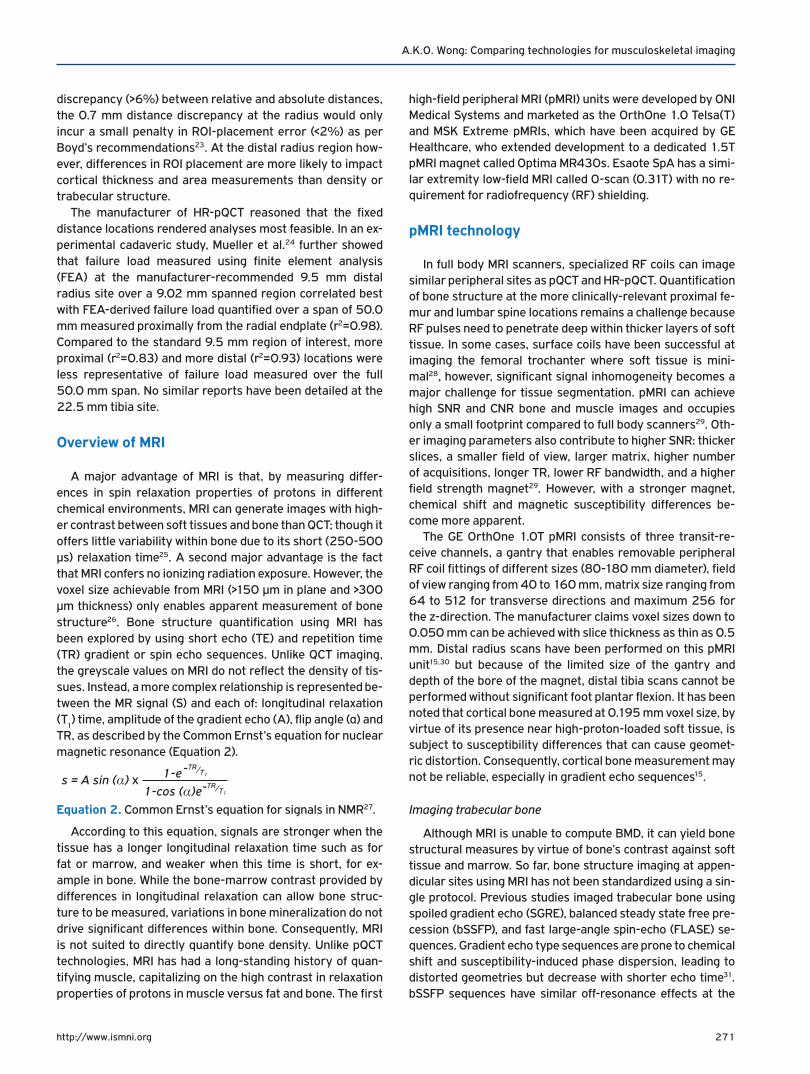
TR, as described by the Common Ernst’s equation for nuclear magnetic resonance (Equation 2).

1-e-TR/T1

s = A sin (α) x -TR/T11-cos (α)e

Equation 2. Common Ernst’s equation for signals in NMR27.

According to this equation, signals are stronger when the tissue has a longer longitudinal relaxation time such as for fat or marrow, and weaker when this time is short, for ex-ample in bone. While the bone-marrow contrast provided by differences in longitudinal relaxation can allow bone struc-ture to be measured, variations in bone mineralization do not drive significant differences within bone. Consequently, MRI is not suited to directly quantify bone density. Unlike pQCT technologies, MRI has had a long-standing history of quan-tifying muscle, capitalizing on the high contrast in relaxation properties of protons in muscle versus fat and bone. The first

high-field peripheral MRI (pMRI) units were developed by ONI Medical Systems and marketed as the OrthOne 1.0 Telsa(T) and MSK Extreme pMRIs, which have been acquired by GE Healthcare, who extended development to a dedicated 1.5T pMRI magnet called Optima MR430s. Esaote SpA has a simi-lar extremity low-field MRI called O-scan (0.31T) with no re-quirement for radiofrequency (RF) shielding.

pMRI technology

In full body MRI scanners, specialized RF coils can image similar peripheral sites as pQCT and HR-pQCT. Quantification of bone structure at the more clinically-relevant proximal fe-mur and lumbar spine locations remains a challenge because RF pulses need to penetrate deep within thicker layers of soft tissue. In some cases, surface coils have been successful at imaging the femoral trochanter where soft tissue is mini-mal28, however, significant signal inhomogeneity becomes a major challenge for tissue segmentation. pMRI can achieve high SNR and CNR bone and muscle images and occupies only a small footprint compared to full body scanners29. Oth-er imaging parameters also contribute to higher SNR: thicker slices, a smaller field of view, larger matrix, higher number of acquisitions, longer TR, lower RF bandwidth, and a higher field strength magnet29. However, with a stronger magnet, chemical shift and magnetic susceptibility differences be-come more apparent.

The GE OrthOne 1.0T pMRI consists of three transit-re-ceive channels, a gantry that enables removable peripheral RF coil fittings of different sizes (80-180 mm diameter), field of view ranging from 40 to 160 mm, matrix size ranging from 64 to 512 for transverse directions and maximum 256 for the z-direction. The manufacturer claims voxel sizes down to 0.050 mm can be achieved with slice thickness as thin as 0.5 mm. Distal radius scans have been performed on this pMRI unit15,30 but because of the limited size of the gantry and depth of the bore of the magnet, distal tibia scans cannot be performed without significant foot plantar flexion. It has been noted that cortical bone measured at 0.195 mm voxel size, by virtue of its presence near high-proton-loaded soft tissue, is subject to susceptibility differences that can cause geomet-ric distortion. Consequently, cortical bone measurement may not be reliable, especially in gradient echo sequences15.

Imaging trabecular bone

Although MRI is unable to compute BMD, it can yield bone structural measures by virtue of bone’s contrast against soft tissue and marrow. So far, bone structure imaging at appen-dicular sites using MRI has not been standardized using a sin-gle protocol. Previous studies imaged trabecular bone using spoiled gradient echo (SGRE), balanced steady state free pre-cession (bSSFP), and fast large-angle spin-echo (FLASE) se-quences. Gradient echo type sequences are prone to chemical shift and susceptibility-induced phase dispersion, leading to distorted geometries but decrease with shorter echo time31. bSSFP sequences have similar off-resonance effects at the



level of trabeculae originating from changes in precession an-gles, but can be decreased by combining images using differ-ent RF pulses32. Spin echo sequences better represent partial volumed voxels as intermediate signal intensities rather than complete signal loss as with gradient echo and bSSFP images, which overestimates bone volume fraction (BV/TV)33. Howev-er, long repetition times are necessary for spin echo sequenc-es. This limitation is addressed by FLASE, which uses sequen-tial pulses to stimulate echoes and minimize saturation, while rephasing and restoring inverted spins34. The resultant imag-es from FLASE exhibit higher SNR compared to gradient echo and SSFP imaging. In any of the sequences described above, BV/TV can be computed but bone density cannot be directly estimated. While Tassani et al showed that tissue mineral den-sity is relatively constant for cortical (1.19±0.06 g/cm3) and trabecular bone (1.24±0.16 g/cm3)35, computing bone den-sity from BV/TV in MR images by assuming this property re-mains inaccurate if voxel sizes are large and significant partial volume artifact is present.

Imaging muscle and fat

By virtue of fat’s lower resonance frequency, shorter spin-lattice and spin-spin relaxation times compared to water, the fat-water chemical shift (3.35 ppm) could generate sufficient contrast to enable muscle-fat segmentation36. It is impor-tant to first acknowledge the differences among: 1) inter-muscular fat (fat between muscle groups), 2) intramuscular fat (fat within muscle groups but still outside muscle cells), 3) extramyocellular lipids (EMCL, outside muscle cells and can include intramuscular fat), and 4) intramyocellular lipids (IMCL, inside muscle cells). Both IMCL and EMCLs can only be measured using oil-red O stained sections from muscle biopsies37, or through MR spectroscopy38, which will not be covered in this review. Basic T

1 or T

2-weighted fast spin echo

(FSE) sequences can depict fine streaks of inter- and intra-muscular fat. Although both methods’ images of muscle and fat appear similar, the latter is sensitive to pathologies that increase water in muscle39. Spin-echo sequences have been criticized for the lack of water exclusion from fat-containing areas. Two-point Dixon adjusts echo times in FSE sequences to yield in-phase (IP) and out-of-phase (OP) images. The fat-only portion can be calculated as ½[IP-OP]40, but is affected by field inhomogeneity which causes artefactual variations in signal intensities across the image. Correction of field inho-mogeneity using bias field estimation methods like phased ar-ray uniformity enhancement (PURE) has improved the Dixon method’s feasibility41. Three-point Dixon applies a third water-fat chemical shift phase encoding step that measures local field differences within voxels, and adjusts for inhomogene-ity using mathematical equations42. More recently, iterative decomposition of water and fat signals with echo asymmetry and least-squares estimation (IDEAL) has been successful in isolating fat by staggering phases of echoes by integer varia-tions of 2π/343,44. These images are not sensitive to field inho-mogeneities and yield high SNR images45. However, water-fat phase swapping is occasionally observed (8.1%, N=283)46,

resulting in replacement with fat where one expects water, and vice versa. For measuring muscle adiposity in the general population, FSE sequences may already be sufficient. Beattie et al showed that inter-muscular (ICC: 0.904) and intra-mus-cular (ICC: 0.844) volumes from FSE agreed closely to those measured using IDEAL images47. However, those with mus-cular disorders such as dystrophies may benefit from more intricate water-fat separation methods.

Voxel size & slice thickness

At 82 µm voxel size, trabecular geometry can only be ap-proximated at best. For a mean trabecular thickness (Tb.Th) of 205.4±29.9 µm, as determined from iliac crest biopsies48, a maximum of two voxels can span across without interrup-tion; an additional two voxels can also span the borders of the trabecular bone. Depending on the anatomy, Tb.Th can range from 50 to 300 µm49. For a sufficiently small voxel size to measure structures accurately, a general rule of thumb is accepted to include at least 3 voxels spanning across the ob-ject width without crossing the borders. Hence, any trabecu-lar thicknesses less than 246 µm (3 voxels at 82 µm each) may be inaccurately measured using HR-pQCT. This limita-tion becomes more serious for pMRI (pixel size: 195 µm) and pQCT (pixel size: 200 µm), which could only include one pixel spanning the trabecular bone at best, manifesting in signifi-cant partial volume effects. Augat et al demonstrated this problem with the limited accuracy of cortical thickness (Ct.Th) and vBMD measurements on pQCT, with the primary cul-prit being partial voluming at the end voxels overlapping bone boundaries, especially in bones with thinner cortices50. This phenomenon explains the inverse relationship observed be-tween cortical bone and marrow density with increasing pixel sizes shown in Table 3. Hangartner also illustrated how peak cortical vBMD is reached only when the width of the structure can be represented by more than 6 pixels across51. To ad-dress this problem, the authors suggested using a segmenta-tion threshold equal to the average between the two tissues to obtain mineral content, and a second but lower threshold to quantify area so as not to overestimate. Compact cortical density varies only to a small degree with exception of pa-tients with osteomalacia. Therefore, it is justifiable to use a fixed threshold to determine cortical density and cortical ge-ometry. Although these two investigations were focused on cortical bone, the same could be extended to trabecular bone. Unlike trabecular bone, the variance in inter- and intramus-cular fat thickness is wider within and between individuals. While larger pixel sizes could preclude the ability to identify thinner streaks of fat, there may be less concern associated with achieving sufficient clinical sensitivity across individuals based on measuring larger fat streaks alone. Though, analyt-ical sensitivity could be improved with smaller voxels leading to enhanced ability to measure changes.

Partial volume artifact resulting from larger slice thick-nesses of pQCT (2.0 mm) followed by pMRI (>0.3 mm) are major culprits for quantifying trabecular geometry and, to a



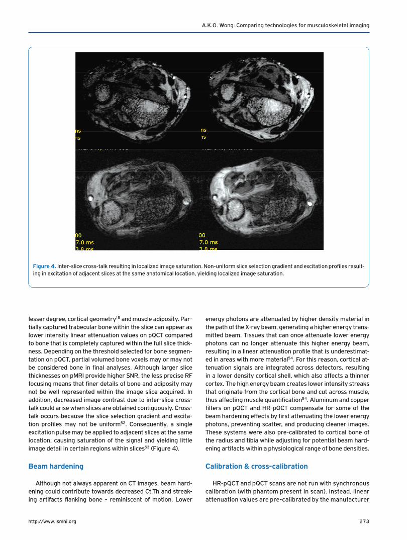
lesser degree, cortical geometry15 and muscle adiposity. Par-tially captured trabecular bone within the slice can appear as lower intensity linear attenuation values on pQCT compared to bone that is completely captured within the full slice thick-ness. Depending on the threshold selected for bone segmen-tation on pQCT, partial volumed bone voxels may or may not be considered bone in final analyses. Although larger slice thicknesses on pMRI provide higher SNR, the less precise RF focusing means that finer details of bone and adiposity may not be well represented within the image slice acquired. In addition, decreased image contrast due to inter-slice cross-talk could arise when slices are obtained contiguously. Cross-talk occurs because the slice selection gradient and excita-tion profiles may not be uniform52. Consequently, a single excitation pulse may be applied to adjacent slices at the same location, causing saturation of the signal and yielding little image detail in certain regions within slices53 (Figure 4).

Beam hardening

Although not always apparent on CT images, beam hard-ening could contribute towards decreased Ct.Th and streak-ing artifacts flanking bone - reminiscent of motion. Lower

energy photons are attenuated by higher density material in the path of the X-ray beam, generating a higher energy trans-mitted beam. Tissues that can once attenuate lower energy photons can no longer attenuate this higher energy beam, resulting in a linear attenuation profile that is underestimat-ed in areas with more material54. For this reason, cortical at-tenuation signals are integrated across detectors, resulting in a lower density cortical shell, which also affects a thinner cortex. The high energy beam creates lower intensity streaks that originate from the cortical bone and cut across muscle, thus affecting muscle quantification54. Aluminum and copper filters on pQCT and HR-pQCT compensate for some of the beam hardening effects by first attenuating the lower energy photons, preventing scatter, and producing cleaner images. These systems were also pre-calibrated to cortical bone of the radius and tibia while adjusting for potential beam hard-ening artifacts within a physiological range of bone densities.

Calibration & cross-calibration

HR-pQCT and pQCT scans are not run with synchronous calibration (with phantom present in scan). Instead, linear attenuation values are pre-calibrated by the manufacturer

Figure 4. Inter-slice cross-talk resulting in localized image saturation. Non-uniform slice selection gradient and excitation profiles result-ing in excitation of adjacent slices at the same anatomical location, yielding localized image saturation.



with calibration equations specific to each scanner, assum-ing this calibration remains stable over time9. By default, fat under pQCT has been assigned a density value of 0 mg/cm3, water with 60 mg/cm3, and the densest compact bone assumed to be 1920 mg/cm3 (58% collagen matrix with density of water 1.0 g/cm3+42% mineral with density of 3.2 g/cm3). All density values computed by pQCT repre-sent measurable apparent or Archimedean bone density9. To circumvent comparability challenges, linear attenua-tion values (µ) on HR-pQCT are standardized to Hounsfield units ((µ

tissue/µ

water-1)*1000 HU), which are then converted

to hydroxyapatite (HA) equivalent density units (mg HA/cm

3) by phantom calibration55. Water on HR-pQCT is as-

sumed to have a value of 0 mg/cm3. Therefore, any densi-tometric comparison between HR-pQCT and pQCT should account for an offset of 60 mg/cm3.

Since MRI is based on differences in proton relaxation properties, it has no calibration to physical densities. Mar-row T

2 relaxation time on MRI has, however, been related

to trabecular vBMD measured on QCT56,57. In addition, Ho et al showed a correlation of 0.98 (p<0.01) between T

2* (transverse relaxation due to neighbouring spins and

magnetic field inhomogeneities i.e. from hemoglobin) from IDEAL sequences and hydroxyapatite concentration in wa-ter; and a correlation of 0.82 between T

2* and physical

density on QCT. However, this technique was only vali-dated on 5 volunteers58. Others reported skeletal muscle mass measurement from MR images by assuming a fixed density of skeletal muscle (1.04 g/cm3)59, but readers are cautioned that these values are neither direct nor accu-rate reflections of physical mass.

While factory pre-calibration provides standardized

physical density measurements for pQCT and HR-pQCT images, calibrating the scanners post-delivery, after any perturbation or re-location of the scanner, and cross-calibration of different scanners are necessary to ensure measurements remain comparable. In multi-centre stud-ies, cross-calibration of scanners is critical to account for differences in pre-calibrated settings, for variable drift in detector performance, and for scatter that may be de-pendent on the environment.

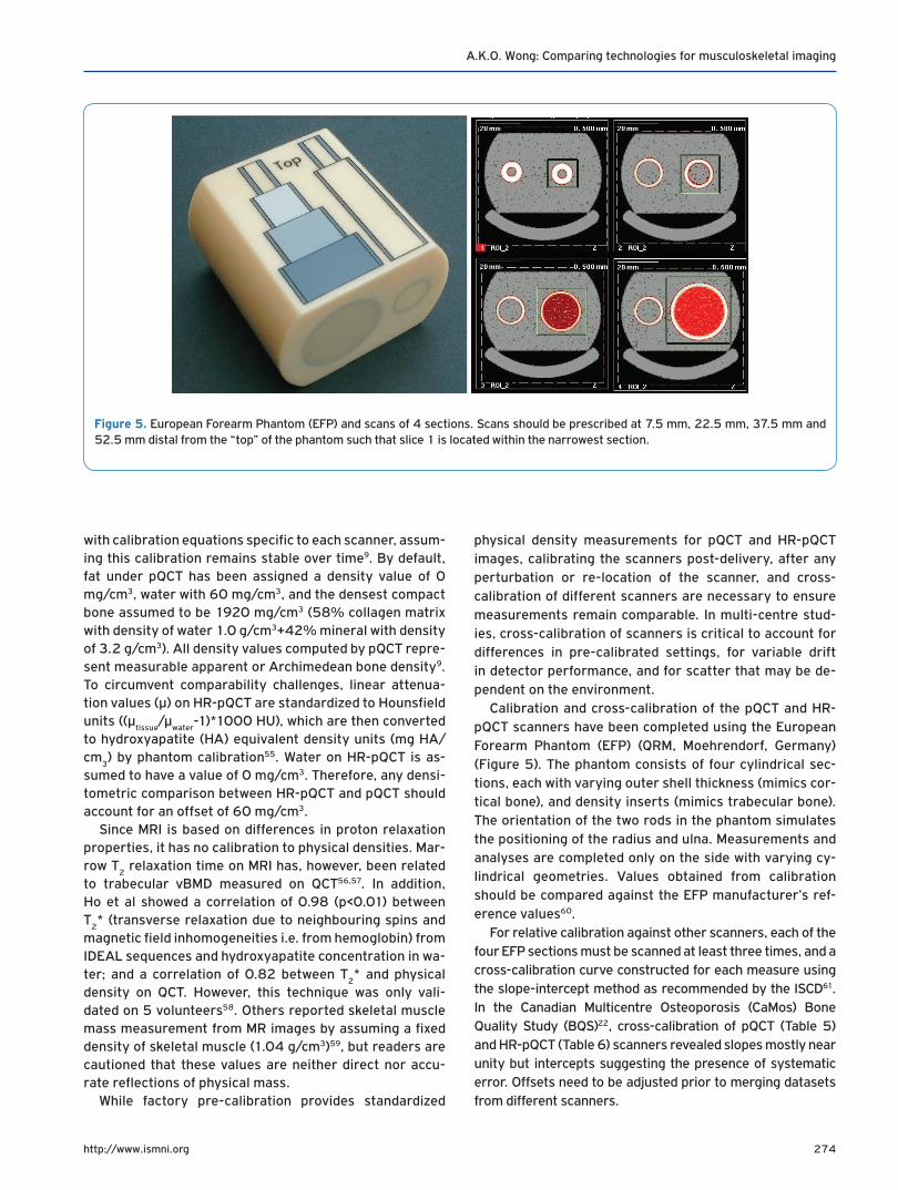
Calibration and cross-calibration of the pQCT and HR-pQCT scanners have been completed using the European Forearm Phantom (EFP) (QRM, Moehrendorf, Germany) (Figure 5). The phantom consists of four cylindrical sec-tions, each with varying outer shell thickness (mimics cor-tical bone), and density inserts (mimics trabecular bone). The orientation of the two rods in the phantom simulates the positioning of the radius and ulna. Measurements and analyses are completed only on the side with varying cy-lindrical geometries. Values obtained from calibration should be compared against the EFP manufacturer’s ref-erence values60.

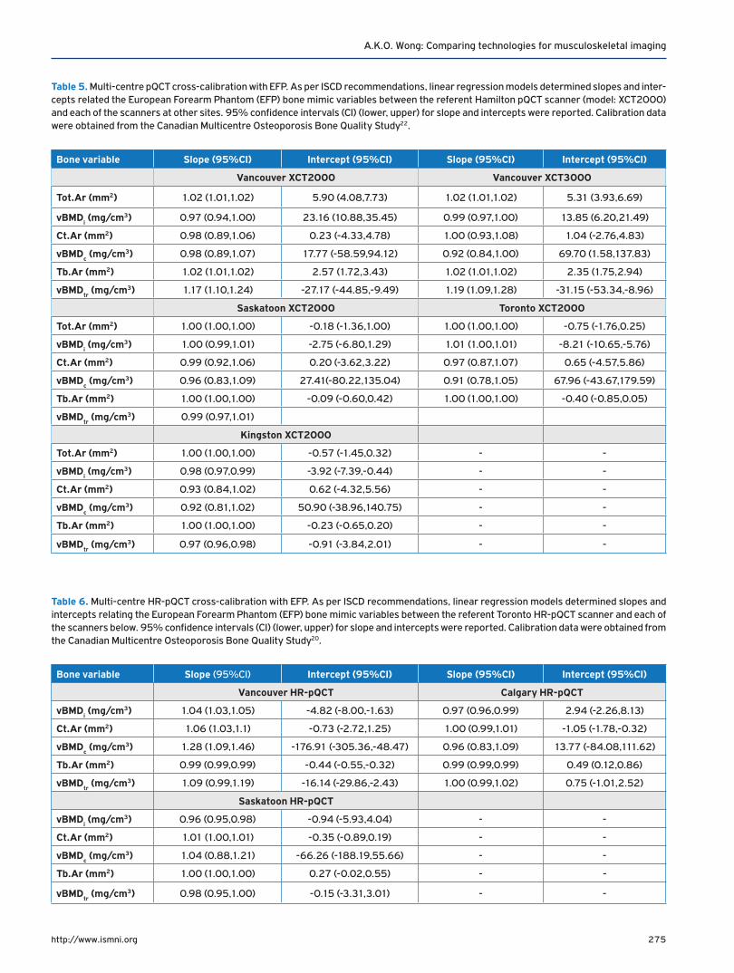
For relative calibration against other scanners, each of the four EFP sections must be scanned at least three times, and a cross-calibration curve constructed for each measure using the slope-intercept method as recommended by the ISCD61. In the Canadian Multicentre Osteoporosis (CaMos) Bone Quality Study (BQS)22, cross-calibration of pQCT (Table 5) and HR-pQCT (Table 6) scanners revealed slopes mostly near unity but intercepts suggesting the presence of systematic error. Offsets need to be adjusted prior to merging datasets from different scanners.

Figure 5. European Forearm Phantom (EFP) and scans of 4 sections. Scans should be prescribed at 7.5 mm, 22.5 mm, 37.5 mm and 52.5 mm distal from the “top” of the phantom such that slice 1 is located within the narrowest section.



Table 5. Multi-centre pQCT cross-calibration with EFP. As per ISCD recommendations, linear regression models determined slopes and inter-cepts related the European Forearm Phantom (EFP) bone mimic variables between the referent Hamilton pQCT scanner (model: XCT2000) and each of the scanners at other sites. 95% confidence intervals (CI) (lower, upper) for slope and intercepts were reported. Calibration data were obtained from the Canadian Multicentre Osteoporosis Bone Quality Study22.

Bone variable Slope (95%CI) Intercept (95%CI) Slope (95%CI) Intercept (95%CI)

Vancouver XCT2000 Vancouver XCT3000

Tot.Ar (mm2) 1.02 (1.01,1.02) 5.90 (4.08,7.73) 1.02 (1.01,1.02) 5.31 (3.93,6.69)

vBMDi (mg/cm3) 0.97 (0.94,1.00) 23.16 (10.88,35.45) 0.99 (0.97,1.00) 13.85 (6.20,21.49)

Ct.Ar (mm2) 0.98 (0.89,1.06) 0.23 (-4.33,4.78) 1.00 (0.93,1.08) 1.04 (-2.76,4.83)

vBMDc (mg/cm3) 0.98 (0.89,1.07) 17.77 (-58.59,94.12) 0.92 (0.84,1.00) 69.70 (1.58,137.83)

Tb.Ar (mm2) 1.02 (1.01,1.02) 2.57 (1.72,3.43) 1.02 (1.01,1.02) 2.35 (1.75,2.94)

vBMDtr (mg/cm3) 1.17 (1.10,1.24) -27.17 (-44.85,-9.49) 1.19 (1.09,1.28) -31.15 (-53.34,-8.96)

Saskatoon XCT2000 Toronto XCT2000

Tot.Ar (mm2) 1.00 (1.00,1.00) -0.18 (-1.36,1.00) 1.00 (1.00,1.00) -0.75 (-1.76,0.25)

vBMDi (mg/cm3) 1.00 (0.99,1.01) -2.75 (-6.80,1.29) 1.01 (1.00,1.01) -8.21 (-10.65,-5.76)

Ct.Ar (mm2) 0.99 (0.92,1.06) 0.20 (-3.62,3.22) 0.97 (0.87,1.07) 0.65 (-4.57,5.86)

vBMDc (mg/cm3) 0.96 (0.83,1.09) 27.41(-80.22,135.04) 0.91 (0.78,1.05) 67.96 (-43.67,179.59)

Tb.Ar (mm2) 1.00 (1.00,1.00) -0.09 (-0.60,0.42) 1.00 (1.00,1.00) -0.40 (-0.85,0.05)

vBMDtr (mg/cm3) 0.99 (0.97,1.01)

Kingston XCT2000

Tot.Ar (mm2) 1.00 (1.00,1.00) -0.57 (-1.45,0.32) - -

vBMDi (mg/cm3) 0.98 (0.97,0.99) -3.92 (-7.39,-0.44) - -

Ct.Ar (mm2) 0.93 (0.84,1.02) 0.62 (-4.32,5.56) - -

vBMDc (mg/cm3) 0.92 (0.81,1.02) 50.90 (-38.96,140.75) - -

Tb.Ar (mm2) 1.00 (1.00,1.00) -0.23 (-0.65,0.20) - -

vBMDtr (mg/cm3) 0.97 (0.96,0.98) -0.91 (-3.84,2.01) - -

Table 6. Multi-centre HR-pQCT cross-calibration with EFP. As per ISCD recommendations, linear regression models determined slopes and intercepts relating the European Forearm Phantom (EFP) bone mimic variables between the referent Toronto HR-pQCT scanner and each of the scanners below. 95% confidence intervals (CI) (lower, upper) for slope and intercepts were reported. Calibration data were obtained from the Canadian Multicentre Osteoporosis Bone Quality Study20.

Bone variable Slope (95%CI) Intercept (95%CI) Slope (95%CI) Intercept (95%CI)

Vancouver HR-pQCT Calgary HR-pQCT

vBMDi (mg/cm3) 1.04 (1.03,1.05) -4.82 (-8.00,-1.63) 0.97 (0.96,0.99) 2.94 (-2.26,8.13)

Ct.Ar (mm2) 1.06 (1.03,1.1) -0.73 (-2.72,1.25) 1.00 (0.99,1.01) -1.05 (-1.78,-0.32)

vBMDc (mg/cm3) 1.28 (1.09,1.46) -176.91 (-305.36,-48.47) 0.96 (0.83,1.09) 13.77 (-84.08,111.62)

Tb.Ar (mm2) 0.99 (0.99,0.99) -0.44 (-0.55,-0.32) 0.99 (0.99,0.99) 0.49 (0.12,0.86)

vBMDtr (mg/cm3) 1.09 (0.99,1.19) -16.14 (-29.86,-2.43) 1.00 (0.99,1.02) 0.75 (-1.01,2.52)

Saskatoon HR-pQCT

vBMDi (mg/cm3) 0.96 (0.95,0.98) -0.94 (-5.93,4.04) - -

Ct.Ar (mm2) 1.01 (1.00,1.01) -0.35 (-0.89,0.19) - -

vBMDc (mg/cm3) 1.04 (0.88,1.21) -66.26 (-188.19,55.66) - -

Tb.Ar (mm2) 1.00 (1.00,1.00) 0.27 (-0.02,0.55) - -

vBMDtr (mg/cm3) 0.98 (0.95,1.00) -0.15 (-3.31,3.01) - -



Image motion assessment

HR-pQCT motion assessment

Motion artifact on HR-pQCT scans are qualitatively as-sessed after reconstruction of images using a scale of 1 to 5, with 1 representing the absence of motion, through criteria that were recommended by the manufacturer62. Although a set threshold for requiring repeat scanning is

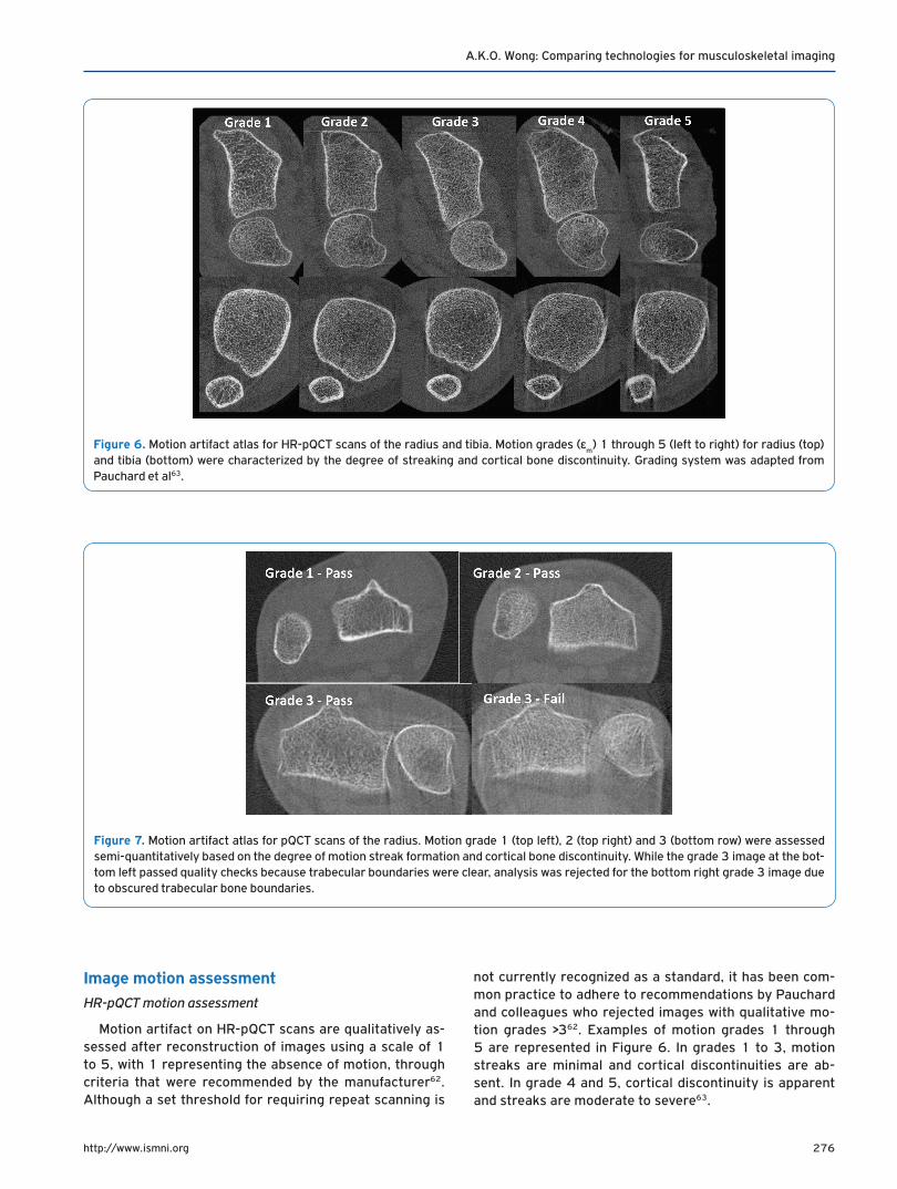
not currently recognized as a standard, it has been com-mon practice to adhere to recommendations by Pauchard and colleagues who rejected images with qualitative mo-tion grades >362. Examples of motion grades 1 through 5 are represented in Figure 6. In grades 1 to 3, motion streaks are minimal and cortical discontinuities are ab-sent. In grade 4 and 5, cortical discontinuity is apparent and streaks are moderate to severe63.

Figure 6. Motion artifact atlas for HR-pQCT scans of the radius and tibia. Motion grades (εm) 1 through 5 (left to right) for radius (top)

and tibia (bottom) were characterized by the degree of streaking and cortical bone discontinuity. Grading system was adapted from Pauchard et al63.

Figure 7. Motion artifact atlas for pQCT scans of the radius. Motion grade 1 (top left), 2 (top right) and 3 (bottom row) were assessed semi-quantitatively based on the degree of motion streak formation and cortical bone discontinuity. While the grade 3 image at the bot-tom left passed quality checks because trabecular boundaries were clear, analysis was rejected for the bottom right grade 3 image due to obscured trabecular bone boundaries.



pQCT motion assessment

pQCT motion assessment has informally been applied by different study groups as a binary grade of pass or fail. Im-ages with discontinuity in the cortical bone are considered to have failed quality checks64. This assessment is consistent

with failing grades 4 and 5 for HR-pQCT images. However, due to the stringent demands for a superior SNR and CNR for trabecular structure computation, separate rules for image quality have been recommended for pQCT15. A semi-quan-titative scale of 1 to 3 for motion severity combined with a binary grade for trabecular bone disruption was formulated

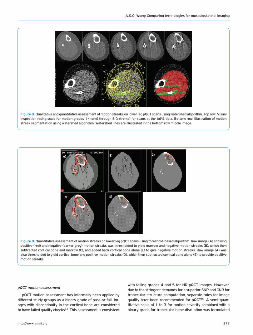
Figure 8. Qualitative and quantitative assessment of motion streaks on lower leg pQCT scans using watershed algorithm. Top row: Visual inspection rating scale for motion grades 1 (none) through 5 (extreme) for scans at the 66% tibia. Bottom row: Illustration of motion streak segmentation using watershed algorithm. Watershed lines are illustrated in the bottom row middle image.

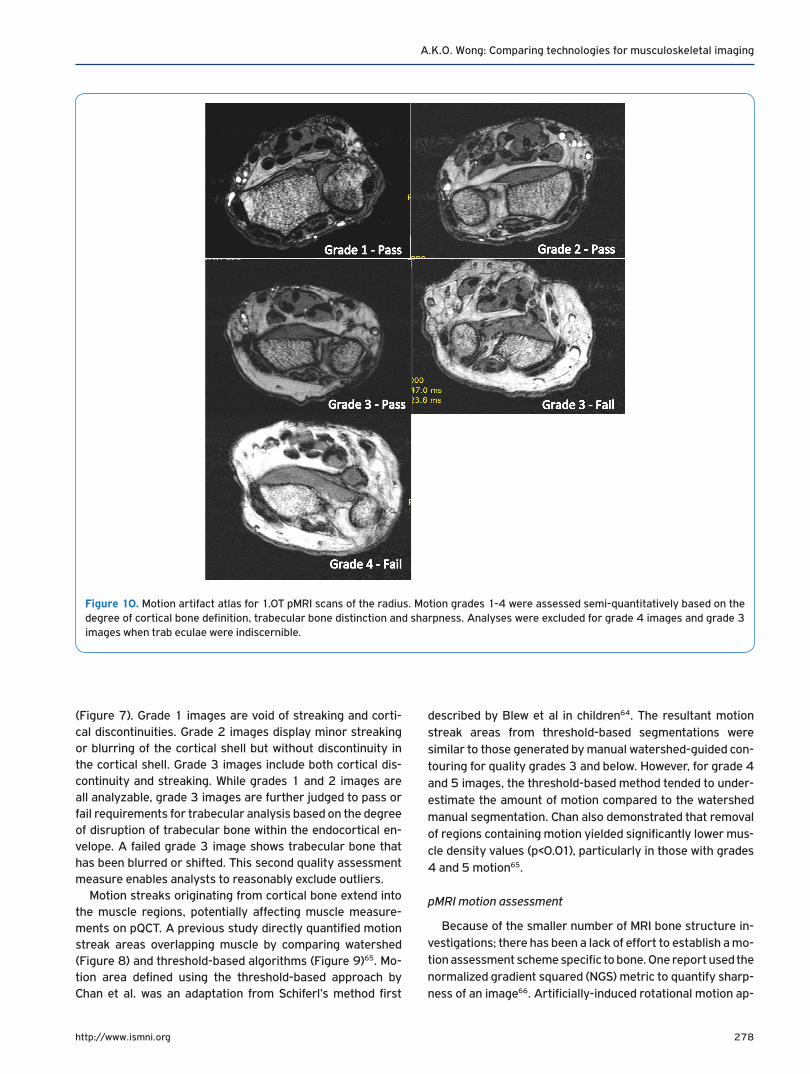
Figure 9. Quantitative assessment of motion streaks on lower leg pQCT scans using threshold-based algorithm. Raw image (A) showing positive (red) and negative (darker grey) motion streaks was thresholded to yield marrow and negative motion streaks (B), which then subtracted cortical bone and marrow (C), and added back cortical bone alone (E) to give negative motion streaks. Raw image (A) was also thresholded to yield cortical bone and positive motion streaks (D), which then subtracted cortical bone alone (E) to provide positive motion streaks.



(Figure 7). Grade 1 images are void of streaking and corti-cal discontinuities. Grade 2 images display minor streaking or blurring of the cortical shell but without discontinuity in the cortical shell. Grade 3 images include both cortical dis-continuity and streaking. While grades 1 and 2 images are all analyzable, grade 3 images are further judged to pass or fail requirements for trabecular analysis based on the degree of disruption of trabecular bone within the endocortical en-velope. A failed grade 3 image shows trabecular bone that has been blurred or shifted. This second quality assessment measure enables analysts to reasonably exclude outliers.

Motion streaks originating from cortical bone extend into the muscle regions, potentially affecting muscle measure-ments on pQCT. A previous study directly quantified motion streak areas overlapping muscle by comparing watershed (Figure 8) and threshold-based algorithms (Figure 9)65. Mo-tion area defined using the threshold-based approach by Chan et al. was an adaptation from Schiferl’s method first

described by Blew et al in children64. The resultant motion streak areas from threshold-based segmentations were similar to those generated by manual watershed-guided con-touring for quality grades 3 and below. However, for grade 4 and 5 images, the threshold-based method tended to under-estimate the amount of motion compared to the watershed manual segmentation. Chan also demonstrated that removal of regions containing motion yielded significantly lower mus-cle density values (p<0.01), particularly in those with grades 4 and 5 motion65.

pMRI motion assessment

Because of the smaller number of MRI bone structure in-vestigations; there has been a lack of effort to establish a mo-tion assessment scheme specific to bone. One report used the normalized gradient squared (NGS) metric to quantify sharp-ness of an image66. Artificially-induced rotational motion ap-

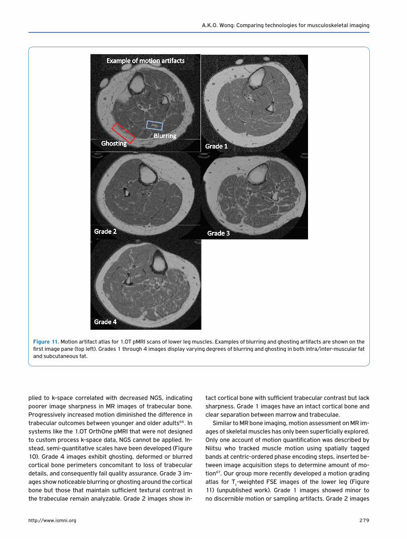
Figure 10. Motion artifact atlas for 1.0T pMRI scans of the radius. Motion grades 1-4 were assessed semi-quantitatively based on the degree of cortical bone definition, trabecular bone distinction and sharpness. Analyses were excluded for grade 4 images and grade 3 images when trab eculae were indiscernible.



plied to k-space correlated with decreased NGS, indicating poorer image sharpness in MR images of trabecular bone. Progressively increased motion diminished the difference in trabecular outcomes between younger and older adults66. In systems like the 1.0T OrthOne pMRI that were not designed to custom process k-space data, NGS cannot be applied. In-stead, semi-quantitative scales have been developed (Figure 10). Grade 4 images exhibit ghosting, deformed or blurred cortical bone perimeters concomitant to loss of trabecular details, and consequently fail quality assurance. Grade 3 im-ages show noticeable blurring or ghosting around the cortical bone but those that maintain sufficient textural contrast in the trabeculae remain analyzable. Grade 2 images show in-

tact cortical bone with sufficient trabecular contrast but lack sharpness. Grade 1 images have an intact cortical bone and clear separation between marrow and trabeculae.

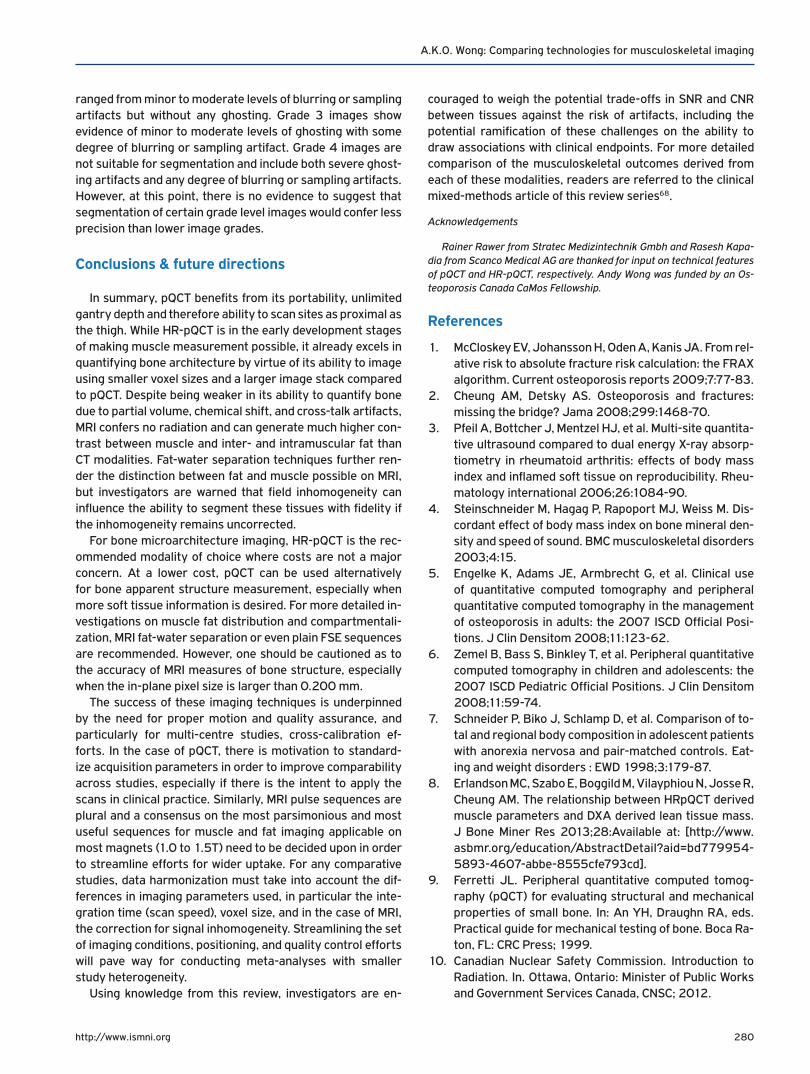
Similar to MR bone imaging, motion assessment on MR im-ages of skeletal muscles has only been superficially explored. Only one account of motion quantification was described by Niitsu who tracked muscle motion using spatially tagged bands at centric-ordered phase encoding steps, inserted be-tween image acquisition steps to determine amount of mo-tion67. Our group more recently developed a motion grading atlas for T

1-weighted FSE images of the lower leg (Figure

11) (unpublished work). Grade 1 images showed minor to no discernible motion or sampling artifacts. Grade 2 images

Figure 11. Motion artifact atlas for 1.0T pMRI scans of lower leg muscles. Examples of blurring and ghosting artifacts are shown on the first image pane (top left). Grades 1 through 4 images display varying degrees of blurring and ghosting in both intra/inter-muscular fat and subcutaneous fat.



ranged from minor to moderate levels of blurring or sampling artifacts but without any ghosting. Grade 3 images show evidence of minor to moderate levels of ghosting with some degree of blurring or sampling artifact. Grade 4 images are not suitable for segmentation and include both severe ghost-ing artifacts and any degree of blurring or sampling artifacts. However, at this point, there is no evidence to suggest that segmentation of certain grade level images would confer less precision than lower image grades.

Conclusions & future directions

In summary, pQCT benefits from its portability, unlimited gantry depth and therefore ability to scan sites as proximal as the thigh. While HR-pQCT is in the early development stages of making muscle measurement possible, it already excels in quantifying bone architecture by virtue of its ability to image using smaller voxel sizes and a larger image stack compared to pQCT. Despite being weaker in its ability to quantify bone due to partial volume, chemical shift, and cross-talk artifacts, MRI confers no radiation and can generate much higher con-trast between muscle and inter- and intramuscular fat than CT modalities. Fat-water separation techniques further ren-der the distinction between fat and muscle possible on MRI, but investigators are warned that field inhomogeneity can influence the ability to segment these tissues with fidelity if the inhomogeneity remains uncorrected.

For bone microarchitecture imaging, HR-pQCT is the rec-ommended modality of choice where costs are not a major concern. At a lower cost, pQCT can be used alternatively for bone apparent structure measurement, especially when more soft tissue information is desired. For more detailed in-vestigations on muscle fat distribution and compartmentali-zation, MRI fat-water separation or even plain FSE sequences are recommended. However, one should be cautioned as to the accuracy of MRI measures of bone structure, especially when the in-plane pixel size is larger than 0.200 mm.

The success of these imaging techniques is underpinned by the need for proper motion and quality assurance, and particularly for multi-centre studies, cross-calibration ef-forts. In the case of pQCT, there is motivation to standard-ize acquisition parameters in order to improve comparability across studies, especially if there is the intent to apply the scans in clinical practice. Similarly, MRI pulse sequences are plural and a consensus on the most parsimonious and most useful sequences for muscle and fat imaging applicable on most magnets (1.0 to 1.5T) need to be decided upon in order to streamline efforts for wider uptake. For any comparative studies, data harmonization must take into account the dif-ferences in imaging parameters used, in particular the inte-gration time (scan speed), voxel size, and in the case of MRI, the correction for signal inhomogeneity. Streamlining the set of imaging conditions, positioning, and quality control efforts will pave way for conducting meta-analyses with smaller study heterogeneity.

Using knowledge from this review, investigators are en-

couraged to weigh the potential trade-offs in SNR and CNR between tissues against the risk of artifacts, including the potential ramification of these challenges on the ability to draw associations with clinical endpoints. For more detailed comparison of the musculoskeletal outcomes derived from each of these modalities, readers are referred to the clinical mixed-methods article of this review series68.

Acknowledgements

Rainer Rawer from Stratec Medizintechnik Gmbh and Rasesh Kapa-dia from Scanco Medical AG are thanked for input on technical features of pQCT and HR-pQCT, respectively. Andy Wong was funded by an Os-teoporosis Canada CaMos Fellowship.

References

1. McCloskey EV, Johansson H, Oden A, Kanis JA. From rel-ative risk to absolute fracture risk calculation: the FRAX algorithm. Current osteoporosis reports 2009;7:77-83.

2. Cheung AM, Detsky AS. Osteoporosis and fractures: missing the bridge? Jama 2008;299:1468-70.

3. Pfeil A, Bottcher J, Mentzel HJ, et al. Multi-site quantita-tive ultrasound compared to dual energy X-ray absorp-tiometry in rheumatoid arthritis: effects of body mass index and inflamed soft tissue on reproducibility. Rheu-matology international 2006;26:1084-90.

4. Steinschneider M, Hagag P, Rapoport MJ, Weiss M. Dis-cordant effect of body mass index on bone mineral den-sity and speed of sound. BMC musculoskeletal disorders 2003;4:15.

5. Engelke K, Adams JE, Armbrecht G, et al. Clinical use of quantitative computed tomography and peripheral quantitative computed tomography in the management of osteoporosis in adults: the 2007 ISCD Official Posi-tions. J Clin Densitom 2008;11:123-62.

6. Zemel B, Bass S, Binkley T, et al. Peripheral quantitative computed tomography in children and adolescents: the 2007 ISCD Pediatric Official Positions. J Clin Densitom 2008;11:59-74.

7. Schneider P, Biko J, Schlamp D, et al. Comparison of to-tal and regional body composition in adolescent patients with anorexia nervosa and pair-matched controls. Eat-ing and weight disorders : EWD 1998;3:179-87.

8. Erlandson MC, Szabo E, Boggild M, Vilayphiou N, Josse R, Cheung AM. The relationship between HRpQCT derived muscle parameters and DXA derived lean tissue mass. J Bone Miner Res 2013;28:Available at: [http://www.asbmr.org/education/AbstractDetail?aid=bd779954-5893-4607-abbe-8555cfe793cd].

9. Ferretti JL. Peripheral quantitative computed tomog-raphy (pQCT) for evaluating structural and mechanical properties of small bone. In: An YH, Draughn RA, eds. Practical guide for mechanical testing of bone. Boca Ra-ton, FL: CRC Press; 1999.

10. Canadian Nuclear Safety Commission. Introduction to Radiation. In. Ottawa, Ontario: Minister of Public Works and Government Services Canada, CNSC; 2012.



11. Sherk VD, Thiebaud RS, Chen Z, Karabulut M, Kim SJ, Bemben DA. Associations between pQCT-based fat and muscle area and density and DXA-based total and leg soft tissue mass in healthy women and men. Journal of musculoskeletal & neuronal interactions 2014;14:411-7.

12. Tang Z, Ho R, Xu Z, Shao Z, Somlyo AP. A high-sensitiv-ity CCD system for parallel electron energy-loss spec-troscopy (CCD for EELS). Journal of microscopy 1994; 175:100-7.

13. Nakamura JK, Schwarz SE. Synchronous Detection vs Pulse Counting for Sensitive Photomultiplier Detection Systems. Applied Optics 1968;7:1073-8.

14. Scanco Medical AG. XtremeCT User’s Guide. Bruetti-sellen, Switzerland; 2005.

15. Wong AK, Beattie KA, Min KK, et al. A Trimodality Com-parison of Volumetric Bone Imaging Technologies. Part I: Short-term Precision and Validity. J Clin Densitom 2014.

16. Zebaze R, Ghasem-Zadeh A, Mbala A, Seeman E. A new method of segmentation of compact-appearing, tran-sitional and trabecular compartments and quantifica-tion of cortical porosity from high resolution periph-eral quantitative computed tomographic images. Bone 2013;54:8-20.

17. Boutroy S, Bouxsein ML, Munoz F, Delmas PD. In vivo as-sessment of trabecular bone microarchitecture by high-resolution peripheral quantitative computed tomogra-phy. J Clin Endocrinol Metab 2005;90:6508-15.

18. Liu D, Burrows M, Egeli D, McKay H. Site specificity of bone architecture between the distal radius and distal tibia in children and adolescents: An HR-pQCT study. Calcif Tissue Int 2010;87:314-23.

19. Burrows M, Liu D, McKay H. High-resolution peripheral QCT imaging of bone micro-structure in adolescents. Osteoporos Int 2010;21:515-20.

20. Burrows M, Liu D, Perdios A, Moore S, Mulpuri K, McKay H. Assessing bone microstructure at the distal radius in children and adolescents using HR-pQCT: a methodo-logical pilot study. J Clin Densitom 2010;13:451-5.

21. Sun L, Beller G, Felsenberg D. Quantification of bone mineral density precision according to repositioning er-rors in peripheral quantitative computed tomography (pQCT) at the radius and tibia. Journal of musculoskel-etal & neuronal interactions 2009;9:18-24.

22. Wong AKO, Berger C, Ioannidis G, et al. The Canadian Mul-ticentre Osteoporosis Bone Quality Study (CaMos BQS): Baseline Comparison of HR-pQCT and pQCT and Frac-ture Associations. J Bone Miner Res 2015;30:#P251.

23. Boyd SK. Site-specific variation of bone micro-archi-tecture in the distal radius and tibia. J Clin Densitom 2008;11:424-30.

24. Mueller TL, Christen D, Sandercott S, et al. Computa-tional finite element bone mechanics accurately pre-dicts mechanical competence in the human radius of an elderly population. Bone 2011;48:1232-8.

25. Fernandez-Seara MA, Wehrli SL, Wehrli FW. Multipoint mapping for imaging of semi-solid materials. Journal of magnetic resonance 2003;160:144-50.

26. Bouxsein ML, Seeman E. Quantifying the material and structural determinants of bone strength. Best practice & research Clinical rheumatology 2009;23:741-53.

27. Ernst R, Anderson W. Application of Fourier transform to magnetic resonance spectroscopy. Rev Sci Instrum 1966;37:93-8.

28. Wehrli FW, Song HK, Saha PK, Wright AC. Quantitative MRI for the assessment of bone structure and function. NMR in biomedicine 2006;19:731-64.

29. Yoshioka H, Schlechtweg P, Kose K. Chapter 3 – Mag-netic Resonance Imaging. In: Weissman B, Caroll C, eds. Imaging of Arthritis and Metabolic Bone Disease. Phila-delphia, PA: Elsevier; 2009.

30. Pritchard JM, Giangregorio LM, Atkinson SA, et al. As-sociation of larger holes in the trabecular bone at the distal radius in postmenopausal women with type 2 diabetes mellitus compared to controls. Arthritis Care & Research 2012;64:83-91.

31. Patton JA. MR imaging instrumentation and image ar-tifacts. Radiographics : a review publication of the Ra-diological Society of North America, Inc 1994;14:1083-96; quiz 97-8.

32. Han M, Chiba K, Banerjee S, Carballido-Gamio J, Krug R. Variable flip angle three-dimensional fast spin-echo sequence combined with outer volume suppression for imaging trabecular bone structure of the proximal femur. Journal of magnetic resonance imaging. JMRI 2015;41:1300-10.

33. Techawiboonwong A, Song HK, Magland JF, Saha PK, Wehrli FW. Implications of pulse sequence in structural imaging of trabecular bone. Journal of magnetic reso-nance imaging. JMRI 2005;22:647-55.

34. Vasilic B, Song HK, Wehrli FW. Coherence-induced arti-facts in large-flip-angle steady-state spin-echo imaging. Magn Reson Med 2004;52:346-53.

35. Tassani S, Ohman C, Baruffaldi F, Baleani M, Viceconti M. Volume to density relation in adult human bone tissue. Journal of Biomechanics 2011;44:103-8.

36. Schick F, Machann J, Brechtel K, et al. MRI of muscular fat. Magn Reson Med 2002;47:720-7.

37. De Bock K, Dresselaers T, Kiens B, Richter EA, Van Hecke P, Hespel P. Evaluation of intramyocellular li-pid breakdown during exercise by biochemical assay, NMR spectroscopy, and Oil Red O staining. American journal of physiology Endocrinology and Metabolism 2007;293:E428-34.

38. Weis J, Johansson L, Ortiz-Nieto F, Ahlstrom H. Assess-ment of lipids in skeletal muscle by LCModel and AM-ARES. Journal of magnetic resonance imaging. JMRI 2009;30:1124-9.

39. Wokke BH, Van Den Bergen JC, Hooijmans MT, Verschu-uren JJ, Niks EH, Kan HE. T2 relaxation times are in-creased in Skeletal muscle of DMD but not BMD patients. Muscle & Nerve 2016;53:38-43.

40. Coombs BD, Szumowski J, Coshow W. Two-point Dixon technique for water-fat signal decomposition with B0 inhomogeneity correction. Magn Reson Med



1997;38:884-9.41. Yang YJ, Park J, Yoon JH, Ahn CB. Field inhomogeneity

correction using partial differential phases in magnetic resonance imaging. Phys Med Biol 2015;60:4075-88.

42. Glover GH, Schneider E. Three-point Dixon technique for true water/fat decomposition with B0 inhomogeneity correction. Magn Reson Med 1991;18:371-83.

43. Reeder SB, Pineda AR, Wen Z, et al. Iterative decompo-sition of water and fat with echo asymmetry and least-squares estimation (IDEAL): application with fast spin-echo imaging. Magn Reson Med 2005;54:636-44.

44. Brodsky EK, Holmes JH, Yu H, Reeder SB. Generalized k-space decomposition with chemical shift correction for non-Cartesian water-fat imaging. Magn Reson Med 2008;59:1151-64.

45. Reeder SB, McKenzie CA, Pineda AR, et al. Water-fat separation with IDEAL gradient-echo imaging. Journal of magnetic resonance imaging. JMRI 2007;25:644-52.

46. Ladefoged CN, Hansen AE, Keller SH, et al. Impact of in-correct tissue classification in Dixon-based MR-AC: fat-water tissue inversion. EJNMMI Physics 2014;1:101.

47. Davison MJ, Maly MR, Adachi JD, Noseworthy MD, Be-attie KA . Relationships between fatty infiltration in the thigh and calf in women with knee osteoarthritis. Aging Clin Exp Res 2016.

48. Beaupied H, Chappard C, Basillais A, Lespessailles E, Benhamou CL. Effect of specimen conditioning on the microarchitectural parameters of trabecular bone as-sessed by micro-computed tomography. Phys Med Biol 2006;51:4621-34.

49. Morgan EF, Barnes GL, Einhorn TA. The Bone Organ Sys-tem: Form and Function. In: Marcus R, Feldman D, Nelson DA, Rosen CJ, eds. Fundamentals of Osteoporosis. San Diego, CA: Elsevier Inc.; 2010:8.

50. Augat P, Gordon CL, Lang TF, Iida H, Genant HK. Accu-racy of cortical and trabecular bone measurements with peripheral quantitative computed tomography (pQCT). Phys Med Biol 1998;43:2873-83.

51. Hangartner TN, Short DF. Accurate quantification of width and density of bone structures by computed to-mography. Medical Physics 2007;34:3777-84.

52. Kneeland JB, Shimakawa A, Wehrli FW. Effect of inter-section spacing on MR image contrast and study time. Radiology 1986;158:819-22.

53. Brown MA, Semelka RC. Extrinsic parameters. In: MRI: Basic Principles and Applications 4th Edition. Hoboken, NJ: John Wiley & Sons; 2010:95.

54. Barrett JF, Keat N. Artifacts in CT: recognition and avoid-ance. Radiographics : a review publication of the Radio-logical Society of North America, Inc 2004;24:1679-91.

55. Boyd SK. Micro-computed tomography. Reconstruc-tions and Caveats. In: Sensen CW, Hallgrimsson B, eds. Advanced Imaging in Biology and Medicine: Technology, Software Environments, Applications. Heidelberg, Ber-lin: Springer-Verlag; 2009. p. 9.

56. Fransson A, Grampp S, Imhof H. Effects of trabecular

bone on marrow relaxation in the tibia. Magnetic reso-nance imaging 1999;17:69-82.

57. Arokoski MH, Arokoski JP, Vainio P, Niemitukia LH, Kr-oger H, Jurvelin JS. Comparison of DXA and MRI meth-ods for interpreting femoral neck bone mineral density. J Clin Densitom 2002;5:289-96.

58. Ho KY, Hu HH, Keyak JH, Colletti PM, Powers CM. Meas-uring bone mineral density with fat-water MRI: compari-son with computed tomography. Journal of magnetic resonance imaging. JMRI 2013;37:237-42.

59. Chen Z, Wang Z, Lohman T, et al. Dual-energy X-ray absorptiometry is a valid tool for assessing skeletal muscle mass in older women. The Journal of Nutrition 2007;137:2775-80.

60. Pearson J, Ruegsegger P, Dequeker J, et al. European semi-anthropomorphic phantom for the cross-calibra-tion of peripheral bone densitometers: a ssessment of precision accuracy and stability. Bone and Mineral 1994;27:109-20.

61. Shepherd JA, Lu Y, Wilson K, et al. Cross-calibration and minimum precision standards for dual-energy X-ray ab-sorptiometry: the 2005 ISCD Official Positions. J Clin Densitom 2006;9:31-6.

62. Pauchard Y, Ayres FJ, Boyd SK. Automated quantifi-cation of three-dimensional subject motion to moni-tor image quality in high-resolution peripheral quan-titative computed tomography. Phys Med Biol 2011; 56:6523-43.

63. Pauchard Y, Liphardt AM, Macdonald HM, Hanley DA, Boyd SK. Quality control for bone quality parameters affected by subject motion in high-resolution periph-eral quantitative computed tomography. Bone 2012; 50:1304-10.

64. Blew RM, Lee VR, Farr JN, Schiferl DJ, Going SB. Stand-ardizing evaluation of pQCT image quality in the pres-ence of subject movement: qualitative versus quantita-tive assessment. Calcif Tissue Int 2014;94:202-11.

65. Chan A, Adachi JD, Papaioannou A, Pickard L, Wong AK. Investigating the effects of motion streaks on the association between pQCT-derived leg muscle den-sity and fractures in older adults. J Bone Miner Res 2015;30:Available at: http://www.asbmr.org/education/ AbstractDetail?aid=c8844053-995d-4768-9263-457296822c3d.

66. Bhagat YA, Rajapakse CS, Magland JF, et al. On the sig-nificance of motion degradation in high-resolution 3D muMRI of trabecular bone. Academic radiology 2011; 18:1205-16.

67. Niitsu M, Campeau NG, Holsinger-Bampton AE, Riederer SJ, Ehman RL. Tracking motion with tagged rapid gradi-ent-echo magnetization-prepared MR imaging. Journal of magnetic resonance imaging. JMRI 1992;2:155-63.

68. Wong AK. A Comparison of Peripheral Imaging Tech-nologies for Bone and Muscle Quantification: a Mixed Methods Clinical Review. Curr Osteoporos Rep 2016; 14(6):359-373.

a comparison of peripheral imaging technologies for bone ... · a comparison of peripheral imaging...

Documents