a comparison of multivariate signal discrimination techniques

This article was downloaded by: [Dicle University]On: 12 November 2014, At: 17:13Publisher: Taylor & FrancisInforma Ltd Registered in England and Wales Registered Number: 1072954 Registeredoffice: Mortimer House, 37-41 Mortimer Street, London W1T 3JH, UK

Journal of Statistical Computation andSimulationPublication details, including instructions for authors andsubscription information:http://www.tandfonline.com/loi/gscs20

A comparison of multivariate signaldiscrimination techniquesRyan F. Schkodaa, Robert Lundb, Nan Sub & John Wagnera

a Department of Mechanical Engineering, Clemson University,Clemson, SC 29634, USAb Department of Mathematical Sciences, Clemson University,Clemson, SC 29634-0975, USAPublished online: 03 Sep 2013.

To cite this article: Ryan F. Schkoda, Robert Lund, Nan Su & John Wagner (2015) A comparison ofmultivariate signal discrimination techniques, Journal of Statistical Computation and Simulation,85:3, 494-506, DOI: 10.1080/00949655.2013.826219

To link to this article: http://dx.doi.org/10.1080/00949655.2013.826219

PLEASE SCROLL DOWN FOR ARTICLE

Taylor & Francis makes every effort to ensure the accuracy of all the information (the“Content”) contained in the publications on our platform. However, Taylor & Francis,our agents, and our licensors make no representations or warranties whatsoever as tothe accuracy, completeness, or suitability for any purpose of the Content. Any opinionsand views expressed in this publication are the opinions and views of the authors,and are not the views of or endorsed by Taylor & Francis. The accuracy of the Contentshould not be relied upon and should be independently verified with primary sourcesof information. Taylor and Francis shall not be liable for any losses, actions, claims,proceedings, demands, costs, expenses, damages, and other liabilities whatsoever orhowsoever caused arising directly or indirectly in connection with, in relation to or arisingout of the use of the Content.

This article may be used for research, teaching, and private study purposes. Anysubstantial or systematic reproduction, redistribution, reselling, loan, sub-licensing,systematic supply, or distribution in any form to anyone is expressly forbidden. Terms &Conditions of access and use can be found at http://www.tandfonline.com/page/terms-and-conditions

http://www.tandfonline.com/loi/gscs20

http://www.tandfonline.com/action/showCitFormats?doi=10.1080/00949655.2013.826219

http://dx.doi.org/10.1080/00949655.2013.826219

http://www.tandfonline.com/page/terms-and-conditions

http://www.tandfonline.com/page/terms-and-conditions

Journal of Statistical Computation and Simulation, 2015Vol. 85, No. 3, 494–506, http://dx.doi.org/10.1080/00949655.2013.826219

A comparison of multivariate signal discrimination techniques

Ryan F. Schkodaa, Robert Lundb*, Nan Sub and John Wagnera

aDepartment of Mechanical Engineering, Clemson University, Clemson, SC 29634, USA; bDepartmentof Mathematical Sciences, Clemson University, Clemson, SC 29634-0975, USA

(Received 20 May 2013; final version received 15 July 2013)

This paper investigates several techniques to discriminate two multivariate stationary signals. The methodsconsidered include Gaussian likelihood ratio tests for variance equality, a chi-squared time-domain test, anda spectral-based test. The latter two tests assess equality of the multivariate autocovariance function of thetwo signals over many different lags. The Gaussian likelihood ratio test is perhaps best viewed as principalcomponent analyses (PCA) without dimension reduction aspects; it can be modified to consider covariancefeatures other than variances via dimension augmentation tactics. A simulation study is constructed thatshows how one can make inappropriate conclusions with PCA tests, even when dimension augmentationtechniques are used to incorporate non-zero lag autocovariances into the analysis. The various discrimina-tion methods are first discussed. A simulation study then illuminates the various properties of the methods.In this pursuit, calculations are needed to identify several multivariate time series models with specificautocovariance properties. To demonstrate the applicability of the methods, nine US and Canadian weatherstations from three distinct regions are clustered. Here, the spectral clustering perfectly identified distinctregions, the chi-squared test performed marginally, and the PCA/likelihood ratio method did not performwell.

Keywords: autocovariance; likelihood ratio; signal equality; spectral analysis

AMS Subject Classifications: 62M10; 62M15

1. Introduction

Given two independent d-dimensional series {Xt} and {Yt} that are preprocessed to a zero-meanstationary setting, this paper considers how to assess whether (or not) the two signals have the sametime series dynamics. This is useful in discrimination and classification pursuits. For example,if a test signal {Yt} is deemed to have different dynamics than a reference signal {Xt} that isknown to be ‘healthy’, then the test signal could be deemed unhealthy. Signal discriminationproblems are fundamental [1,2] and are well-developed when discriminating series via meansor first moments. Here, Hotelling’s T 2 and Q statistics are frequently relied upon.[3,4] In 1986,Coates and Diggle [5] considered discrimination of two constant-mean univariate series basedon their sample autocovariances. Speech signals, for example, are typically of constant mean,regardless of what words are being spoken. Here, word-to-word changes are best identified throughautocovariance shifts and mean analyses are insufficient to identify dynamic changes. In [6], theissue resided with discriminating an earthquake from a covert underground nuclear test; again,the issues involved discrimination of constant-mean data.

*Corresponding author. Email: [email protected]

© 2013 Taylor & Francis

Dow

nloa

ded

by [

Dic

le U

nive

rsity

] at

17:

13 1

2 N

ovem

ber

2014

Journal of Statistical Computation and Simulation 495

The classical way of discriminating {Xt} and {Yt} from second-order characteristics examines aGaussian likelihood ratio. Such a test compares the sample variance matrix of the two series. Elab-orating, conclusions are based on the similarities/differences between the two sample variancematrices

N−1N∑

t=1

XtX′t , N−1

N∑t=1

YtY′t .

Section 2 reviews this likelihood ratio test. Here, N denotes the sample length of the two series,which are assumed equal for convenience. When the dimension d is large, this comparison is typi-cally made after a preliminary dimension reduction transformation, usually some type of principalcomponent analysis (PCA). Without dimension reduction aspects, covariance comparisons are nottruly PCA techniques; however, they share the commonality in that conclusions are based onlyon the sample variances.

Basing signal equality conclusions exclusively on sample variances can produce erroneousconclusions when the two series are not multivariate white noise. A more comprehensive test,discussed further in Section 2, compares the sample autocovariances

�̂X(h) = 1

N

N−h∑t=1

Xt+hX′t , �̂Y(h) = 1

N

N−h∑t=1

Yt+hY′t (1)

over all suitable lags h ≥ 0. Such tests for multivariate series were discussed in [6–8], and thereferences within.

PCA methods have been extended to handle cases where correlation at non-zero lags is present.This is typically done through a dimension augmentation scheme. For example, if �X(1) and/or�Y(1) are believed to be non-zero, one could compare the sample covariance matrices of the2d-dimensional vectors {X∗

t } and {Y∗t }, where X∗

t = (X2t−1,1, . . . , X2t−1,d , X2t,1, . . . , X2t,d)′ and

Y∗t = (Y2t−1,1, . . . , Y2t−1,d , Y2t,1, . . . , Y2t,d)

′. If the sample variance of {X∗t } and {Y∗

t } agrees, thenone concludes that �X(0) = �Y(0) and �X(1) = �Y(1). Higher order comparisons are constructedvia analogous reasoning. Of course, such dimension augmentation tactics shorten the observedseries length; also, there is no clear augmentation dimension when autocovariances at all lags arenon-zero, the typical case in practice.

In [7,8], the problem is attacked with different techniques. Mathematically, two stationarymultivariate covariance functions are equal over all lags if and only if their spectral densities areequal at all frequencies (the spectrum is assumed to have no point masses). From this, signalequality tests that compare the periodograms of both series were devised (Section 2 elaborates).This paper revisits these methods and shows how one can fool variance-based tests for signalequality, even when the dimension is augmented to account for non-zero autocovariances at higherlags. The pros and cons of the various methods are demonstrated by simulating seven multivariatestationary signals with strategically constructed properties and then applying the tests. As anapplication, nine weather stations from the USA and Canada are clustered to determine similarand unsimilar stations.

The rest of this paper proceeds as follows. Section 2 overviews the signal processing back-ground needed. Section 3 then shows how the techniques compare on data simulated from sevenstrategically selected multivariate time series models. Section 4 analyses nine three-dimensionalweather time series containing temperature and wind speeds. Section 5 summarizes the contentof the paper and makes some closing remarks.

Dow

nloa

ded

by [

Dic

le U

nive

rsity

] at

17:

13 1

2 N

ovem

ber

2014

496 R.F. Schkoda et al.

2. Background

We work with two zero-mean d-dimensional covariance stationary signals {Xt} and {Yt} observedat the times t = 1, . . . , N . The covariances (theoretical) at lag h ≥ 0 are �X(h) = E[Xt+hX′

t] and�Y(h) = E[Yt+hY′

t]; we call these quantities variance matrices at lag h = 0.

2.1. Testing equality of variance matrices

The classical test for signal equality of zero-mean stationary series merely compares the samplevariance matrices of the two observed series. The null hypothesis is that �X(0) = �Y(0). AGaussian likelihood ratio statistic for testing this hypothesis is

λ =(

2d det[�̂X(0)�̂Y(0)]1/2

det[�̂X(0) + �̂Y(0)]

)N

,

where det denotes matrix determinant. This statistic is derived in [9, p.404]. The values of λ

are in [0, 1] and the null hypothesis is rejected when λ is too small to be explained by randomchance. Authors have used this test when the series are non-Gaussian white noise without drasticperformance degradations. Here, the usual central limit caveat applies: the test works well for largeN , provided marginal distributions of the series are not heavy-tailed. Applying the test when thedata are autocorrelated (i.e. not white noise) is more problematic. This issue will be investigatedfurther in the next section.

In this setting, −2 log(λ) has an asymptotic (as N → ∞) chi-squared distribution (see [10,11]for generalities). The degrees of freedom is the number of parameters that are saved when thetwo signals have the same variance matrix. Since the variance matrix of a d-dimensional signal isa d × d symmetric matrix, d(d + 1)/2 free parameters are needed to quantify it and d(d + 1)/2parameters are saved when the two variance matrices coincide. In other words, d(d + 1)/2 is theappropriate degrees of freedom.

2.2. Testing equality of the autocovariance functions

A spectral approach to testing equality of multivariate autocovariance functions was developedin [7]. Since �X(h) = �Y(h) for all lags h ≥ 0 if and only if fX(ω) = fY(ω) for all frequenciesω ∈ [0, 2π) (with respect to the Lebesgue measure), where

fX(ω) = 1

2π

∞∑h=−∞

�X(h) e−iωh, fY(ω) = 1

2π

∞∑h=−∞

�Y(h) e−iωh

are the theoretical spectral densities of {Xt} and {Yt} at frequency ω, respectively.In [7], the spectral densities of the two series are statistically compared via their ratios.

Specifically, the discrete Fourier transforms (DFTs) of the series are first computed via

JX(ωj) = N−1/2N∑

t=1

Xt e−itωj , JY(ωj) = N−1/2N∑

t=1

Yt e−itωj

at all Fourier frequencies ωj = 2π j/N , for j = 0, . . . , N − 1 (see [12,13] for Fourier transformbasics). The raw (unsmoothed) spectral densities are estimated via

f̂X(ωj) = JX(ωj)J∗X(ωj)

2π, f̂Y(ωj) = JY(ωj)J∗

Y(ωj)

2π.

Dow

nloa

ded

by [

Dic

le U

nive

rsity

] at

17:

13 1

2 N

ovem

ber

2014


Here, the asterisk denotes complex conjugation. The raw spectral estimates are then smoothedin a uniform manner over the 2M + 1 Fourier frequencies closest to the Fourier frequency beingconsidered:

f̂s

X(ωj) =∑M

k=−M f̂X(ωj+k)

2M + 1, f̂

s

Y(ωj) =∑M

k=−M f̂Y(ωj+k)

2M + 1.

Here, M is a positive integer, representing a smoothing bandwidth, that satisfies 2M + 1 ≥ d(this ensures a finite variance of the smoothed spectral density estimates). The choice of M doesnot usually influence practical conclusions about signal equality, but it is not an easy parameterto optimally select. In smoothing the raw spectral estimates, frequencies outside of [0, 2π) arerounded modulo 2π to mimic the periodic nature of the DFT; for example, f̂X(ωj+N ) = f̂X(ωj).

Signal equality conclusions in [7] are based on the statistic

�̄ = 1

N/2 − 1

N/2−1∑j=1

|�(ωj)|. (2)

Here, the �(λj)s are the log determinant of the ratios of the smoothed spectral density estimates:

�(ωj) = log(det(f̂ sX(ωj))) − log(det(f̂ s

Y(ωj))). (3)

Under the null hypothesis of equal autocovariance functions, �(ωj) should be statistically close tozero for every non-zero Fourier frequency ωj. The fact that �(ωj) has an asymptotic distributionthat does not depend on j for j = 1, 2, . . . , N/2 − 1 or the common spectral density of {Xt} and{Yt} is justified in [7]. From this structure, a test for signal equality based on �̄ is easily constructedfrom the central limit theorem (the �(ωj)s for varying j are approximately independent). Such atest rejects equality of autocovariance functions when

�̄ > μM + zα

σM√N/2 − 1

. (4)

Here, zα is the usual (1 − α)th quantile of the standard normal distribution and μM and σM arethe theoretical mean and variance of |�(ωj)|. Note that this is a one-sided test.

The constantsμM andσ 2M depend on both M and d and are difficult to derive. Explicit expressions

for these constants are derived in [8] when d = 1, but the computations for the multidimensionalcase are intense. However, simulations with Gaussian white noise readily provide good estimatesof them. These estimates are given in tables in [7].

The detection power of the �̄ statistic can be increased if the signals are known to be band-limited. Specifically, if the spectrums of {Xt} and {Yt} are known to be limited to the interval[ωL, ωU ], then Equation (2) is best modified to

�̄ = r−1∑

j:ωj∈[ωL ,ωU ]|�(ωj)|,

where r is the number of distinct Fourier frequencies in the interval [ωL, ωU ]. The rejection regionis the same as in Equation (4), except that N/2 − 1 is replaced by r. Of course, one should take rlarge enough to induce asymptotic normality of averages. Detection power increases because manyfrequencies where no differences occur are excluded in the analysis, accentuating the importanceof differences in the frequency increments that are considered.

A time-domain approach to testing equality of stationary multivariate autocovariance functionswas also developed in [7]. The statistic is χ2 in nature and is based on the joint asymptotic normality

Dow

nloa

ded

by [

Dic

le U

nive

rsity

] at

17:

13 1

2 N

ovem

ber

2014


of the sample autocovariances in Equation (1) (see [14] for asymptotic normality issues). Let

Ci,j(h) = �̂X(h)i,j − �̂Y(h)i,j

be the difference between the sample autocovariances {Xt} and {Yt} for components i and j atlag h, where 1 ≤ i, j ≤ d. A χ2 test is constructed from the information contained in the lagsh = 0, 1, . . . , L for some fixed natural number L as follows. When h = 0, �̂X(0) and �̂Y(0) aresymmetric variance matrices, with d(d + 1)/2 non-repeated entries. For lags h = 1, . . . , L, thematrices �̂X(h) and �̂Y(h) are unconstrained and have d2 non-repeated entries. Adding theseparameter counts, our chi-squared test will have Ld2 + d(d + 1)/2 degrees of freedom.

The chi-squared test has the form

χ2 = n

2C′W−1C,

where C is a Ld2 + d(d + 1)/2-dimensional vector that stacks the unconstrained ele-ments in the sample autocovariances and W is its asymptotic covariance matrix. Elab-orating, C takes its first d(d + 1)/2 components from the variance matrices, stacked inthe order C1,1(0), C1,2(0), . . . , C1,d(0); C2,2(0), . . . , C2,d(0); . . . ; Cd,d(0). The next d2 entriesof C are for the lag 1 covariances and are stacked in the usual row–column orderC1,1(1), . . . , C1,d(1); C2,1(1), . . . , C2,d(1); . . . ; Cd,1(1), . . . , Cd,d(1). The d2 entries for lags2, . . . , L are appended in C similar to the scheme for lag 1. The asymptotic covariance matrixW contains scaled asymptotic covariances between the components in C. Specifically, the scaledasymptotic covariance between Ci,j(h) and Ci′,j′(h′) needed is

limn→∞ n Cov(Ci,j(h), Ci′,j′(h

′)) = limn→∞ n Cov(�̂X(h)i,j, �̂X(h′)i′,j′)

+ limn→∞ n Cov(�̂Y(h)i,j, �̂Y(h′)i′,j′). (5)

Formulas for the terms in Equation (5) are based on Bartlett’s classic asymptotic formula [14] andare listed in Equation (14) of [7] for the general case and Equation (15) of [7] for the Gaussiancase.

The null hypothesis that the two series have the same autocovariances at lags 0, . . . , L is rejectedwhen the χ2 statistic is too large to be explained by chance variation.

Tuning (smoothing) parameters need to be selected in the above tests – M in the spectral test andL in the χ2 test. Optimal guidance is largely unknown. Both of these parameters should dependon the sample size N – say M(N) and L(N). On technical grounds for vector autoregressions,one needs M(N) and L(N) go to infinity as N → ∞, and M(N)/N and L(N)/N to converge tozero as N → ∞. For a vector moving-average of order q, take L = q. In practical applications,the selection of L has been more problematic than that of M.

3. Method comparison

This section studies the properties of the λ, �̄, and χ2 statistics via simulation. Much of ourwork involves locating stationary multivariate time series models with specific autocovariancestructures. In all cases, the issues are apparent with dimension d = 2, Gaussian data, and 95%statistical confidence. The smoothing parameters M = 3 and M = 7 are reported for the �̄ statisticand L = 1, 5, and 25 for the χ2 statistic. The series length N = 1024 is common to all cases; also,one hundred thousand simulations were conducted in all comparisons.

Dow

nloa

ded

by [

Dic

le U

nive

rsity

] at

17:

13 1

2 N

ovem

ber

2014


Table 1. Method and detection powers.

λ �̄(M = 3) �̄(M = 7) χ2(L = 1) χ2(L = 5) χ2(L = 25)

Case I 5.14% 5.54% 5.63% 4.79% 4.39% 3.01%Case II 57.69% 6.64% 7.47% 42.22% 23.04% 8.02%Case III 19.04% 5.30% 5.45% 4.85% 4.42% 6.24%Case IV 73.19% 5.65% 5.95% 6.73% 20.56% 8.94%Case V 8.12% 100.00% 100.00% 100.00% 100.00% 100.00%Case VI 100.00% 100.00% 100.00% 100.00% 100.00% 100.00%Case VII 7.68% 12.36% 18.11% 4.87% 16.17% 5.91%

First, the λ, �̄, and χ2 statistics were computed for the simple case where both {Xt} and {Yt}are zero-mean Gaussian white noise. In this case, the covariance matrix of {Xt} and {Yt} wastaken as the two-dimensional identity matrix. Hence, this case, which we refer to as Case I, is ascenario where the two signals have the same dynamics. Table 1 shows empirically aggregatedproportions of runs where the λ, �̄, and the χ2 test reject the null hypothesis of signal equalityat level 5%. As the proportions are close to 5%, all methods have worked well in this case. Thissaid, the Type-I error of the χ2 test with L = 25 seems to be slightly below 5%. Of course, samplecovariances at high lags are slightly biased, perhaps affecting the χ2 test with large L.

Our second case is one where {Xt} and {Yt} do not have the same variance matrix. Here, {Xt}and {Yt} are zero-mean Gaussian white noise with the variance matrices

�X(0) =[

1.0 0.00.0 1.0

], �Y(0) =

[1.1 0.10.1 1.0

],

respectively. Table 1 displays the proportions of times the λ, �̄, and χ2 tests reject signal equalityat confidence 95%. In this case, the likelihood ratio statistic λ has worked best as seen by itslarger empirical rejection proportion. The χ2 test with L = 1 performs second best. This is notunexpected: while all methods should ideally reject signal equality, the two signals differ onlyin their variances; covariances at all higher lags are zero. While the λ statistic focuses solelyon variance differences, the �̄ test considers all covariance lags and the χ2 test considers lags0, . . . , L. The detection power of the χ2 test degrades with large L as it is mixing in many lagswhere covariance differences are not present.

Case III considers a situation where {Xt} and {Yt} have the same variances, but where there isnon-zero autocorrelation at non-zero lags; that is, the series under consideration are not multivari-ate white noise. We do this by examining solutions to the vector autoregressive moving-average(VARMA) model of autoregressive order two and moving-average order one. Specifically, both{Xt} and {Yt} obey the VARMA difference equation

Xt = �1Xt−1 + �2Xt−2 + Zt + �1Zt−1.

Here, the VARMA matrix coefficients were chosen as

�1 =[

0.40 0.050.05 0.30

], �2 =

[−0.48 0.100.10 −0.06

], �1 =

[0.30 0.100.10 0.50

].

Also, {Zt} is chosen as white noise with an identity covariance matrix. The Case III performancecharacteristics reverse from Case II with the λ statistic erroneously rejecting signal equality about19% of the time. This false alarm rate is unacceptable in a 95% test. The �̄ and χ2 statistics,however, reject signal equality at approximately the intended 5% rate.

Case IV represents an exacerbated version of Case III where we press VARMA stability issues.Here, the two series are taken as vector autoregressions of order one. Specifically, both series

Dow

nloa

ded

by [

Dic

le U

nive

rsity

] at

17:

13 1

2 N

ovem

ber

2014


follow the VAR(1) dynamics

Xt = �Xt−1 + Zt ,

where {Zt} is taken as Gaussian white noise with the identity covariance matrix and

� =[

0.90 0.10−0.10 0.90

].

The autoregressive (AR) coefficient of this model lies near the boundary of the multivariatecausality region of a VAR(1) model, as is seen by the near unit diagonal entries in �. In thiscase, the λ statistic erroneously rejects signal equality at a whopping 73% rate. The �̄ tests hasperformed well. The false alarm (Type-I error) of the χ2 test is also unacceptably larger than thespecified 5%, especially when L = 5. The last two cases show that likelihood ratio tests performpoorly unless the signals are known to be white noise. At this point, one can also question thedetection power of the �̄ and χ2 statistics as they performed poorly in some Case II, where thesignals were truly different.

Case V constructs a situation designed to fool the λ statistic. Specifically, our {Xt} is taken asthe first-order moving-average satisfying

Xt = Zt + �Zt−1,

and {Yt} is taken as white noise Yt = �t . The caveat here is that we select the parameters �,Var(Zt) = �Z, and Var(�t) = �� so that �X(0) = �Y(0). To do this, we take

� =[

0.70 0.300.30 0.50

], �Z =

[1.00 0.000.00 1.00

], �� =

[1.58 0.360.36 1.34

].

In this case, the two series have different dynamics, but have the same lag-zero variance matrix.The empirical probabilities in Table 1 reflect this property: the λ statistic rejects equivalent signaldynamics only slightly more than the 5% nominal false alarm rate; however, the �̄ and χ2 statisticsmake the correct conclusion of signal inequality in all of the one hundred thousand runs.

Overall, the λ test degrades under correlation but is more powerful at detecting variance changeswhen in truth only variance changes are truly present. The χ2 test has problems when the autore-gressive polynomial has roots near the unit circle, and while the �̄ test is not easily fooled, it wasnot very powerful in Case II.

One can reduce equality of autocovariance problems to variance comparisons through dimen-sion augmentation techniques. For example, suppose that the signal’s autocovariances are onlynon-zero at lags 0, 1, . . . , κ and set

X∗n = (X′

(n−1)(κ+1)+1, . . . , X′n(κ+1))

′.

Then, {Xt} and {Yt} have the same autocovariances at lags h = 0, . . . , κ if {X∗n} and {Y∗

n}have equal variances. For example, in Case V, X∗

t = (X2t−1,1, X2t−1,2, X2t,1, X2t,2)′ and Y∗

t =(Y2t−1,1, Y2t−1,2, Y2t,1, Y2t,2)

′. Of course, such tactics may not represent an efficient way ofproceeding when κ is large as series sample sizes are reduced.

Case VI shows empirical probabilities of signal equality rejection when four-dimensional vec-tors are made to analyse the signals generated in Case V. We will not rerun the �̄ and χ2 analyses,preferring to emphasize that the �̄ and χ2 methods naturally handle autocorrelation and that thereis no need to do any sort of dimension augmentation. The rejection probability of the λ statisticin Case V increases to 100% when the dimension is augmented to four. Since moving averages oforder one are completely characterized by their lag-zero and lag-one autocovariances, dimensionaugmentation works very well here.

Dow

nloa

ded

by [

Dic

le U

nive

rsity

] at

17:

13 1

2 N

ovem

ber

2014


Selection of the dimension to augment by is problematic. If one selects the augmentationdimension too small, then the higher order covariances will not be considered (which is suboptimalif these autocovariances are non-zero). On the other hand, if the selected dimension is too large,then the sample size becomes significantly smaller and discrimination power is lost.

Our last case is intended to show that there are no easy ways of selecting augmentation dimen-sions. We do this by constructing two series where the signals have different dynamics, but whereboth the lag-zero and lag-one autocovariances agree. That is, we want {Xt} and {Yt} to have differ-ent dynamics, but �X(0) = �Y(0) and �X(1) = �Y(1). Case VII shows signal equality rejectionprobabilities for this case. This was done by mixing two univariate signals with equal lag-zeroand lag-one autocovariances. Specifically, suppose that {X∗

t,1}, and {X∗t,2}, the components of {X∗

t },both follow the same AR(1) dynamics

X∗t,1 = φX∗

t−1,1 + Zt,1, X∗t,2 = φX∗

t−1,2 + Zt,2,

where {Zt,1} and {Zt,2} are independent zero-mean unit-variance Gaussian white noises. Hence,the two components of {X∗

t } are independent AR(1) series having the same univariate covariancesat all lags. Now suppose that both components of {Y∗

t } obey the same MA(1) dynamics:

Y∗t,1 = ηt,1 + θηt−1,1, Y∗

t,2 = ηt,2 + θηt−1,2,

where {ηt,1} and {ηt,2} are independent zero-mean variance σ 2η Gaussian white noise series. A

computation shows that {X∗t,1} and {Y∗

t,1} have the same lag-zero and lag-one autocovarianceswhen

φ = θ

1 + θ2, σ 2

η = 1 + θ2

1 + θ2 + θ4.

To mix the two components (so that {Xt,1} and {Xt,2} are not independent), set

Xt = L(

X∗t,1

X∗t,2

), Yt = L

(Y∗

t,1Y∗

t,2

),

where

L =[ 1

213− 1

312

].

Then, {Xt} and {Yt} have different signal dynamics, yet, by construction, �X(0) = �Y(0) and�X(1) = �Y(1).

The Case VII probabilities use φ = 14 . The values θ = 2 − √

3 and σ 2η = 0.9952 were chosen to

satisfy the above constraints. Table 1 rejection proportions show that while the �̄ and χ2 statisticsdo not detect signal inequality well, the λ statistic is essentially completely fooled. Because ofthis, we do not consider comparing signals whose autocovariances match to a higher number oflags as the pattern is clear: the λ statistic will have more difficulty correctly discriminating suchsignals.

Overall, the �̄ tests seems to perform well without the need for dimension augmentation. Theχ2 test was often reliable, but its performance varied greatly with L. This smoothing parameteris difficult to select. Again, if the series being compared are known to be moving-averages oforder q, then one should take L = q. Beyond this, however, there seems to be little good guidance.Performance of the likelihood ratio for the equal variance test can degrade, should autocorrelationsin the series be present. (i.e. this test performs well for white noise discrimination only).We suggestthat the �̄ and χ2 statistics be considered, should conclusions on signal equality have importance.

Dow

nloa

ded

by [

Dic

le U

nive

rsity

] at

17:

13 1

2 N

ovem

ber

2014


Figure 1. Station locations.

4. Climate data analysis

To illustrate the utility of the proposed techniques, a climatological data set of nine stations will beclustered. The stations each contain three-dimensional weather time series and were extracted fromthe twentieth Century ReanalysisV2 data at http://www.esrl.noaa.gov/psd/. The three componentsof each series are temperature, meridional wind velocity, and zonal wind velocity, with each entryrepresenting a monthly average of the variable being studied. The data from each site span January1871–December 2010. Nine locations from the USA and Canada, representing three distinctgeographic clusters, are considered: Augusta, GA; Anderson, SC; Athens, GA; Burlington, VT;Kingston, RI; Rochester, NY; Eugene, OR; Seattle, WA; and Vancouver, CAN. Figure 1 depictsthe station locations.

Figure 2 shows a representative segment of all three components from the Anderson, SouthCarolina series. Only a portion of the data is shown for clarity. These data are obviously non-stationary, with temperatures having a clear seasonal mean and variance cycle (wintertimetemperatures are colder and more variable than summertime temperatures). Hence, the seriesshould be preprocessed or transformed to stationarity before applying stationary methods.

Our preprocessing will simply subtract a monthly mean for each component and divide by amonthly standard deviation. This simple tactic is shown to frequently stationarize climatic timeseries.[15] Figure 3 shows the data in Figure 2 after this ‘seasonal standardization’. Of course,such preprocessing eliminates information that could be useful in discrimination and classificationpursuits; in particular, all of the standardized series have a zero mean and unit variance. However,we will see that the λ and C statistics can still effectively see differences in the series from thethree regions.

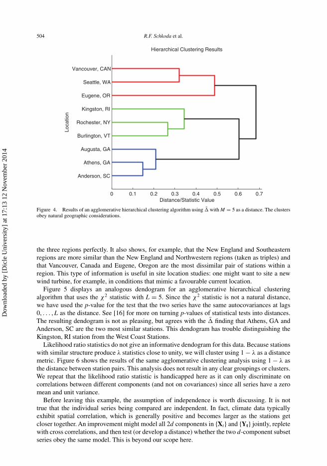
Figure 4 displays a dendogram for an agglomerative hierarchical clustering algorithm thatuses the �̄ statistic with M = 5 as a distance. The �̄ statistic is a natural distance between twostations as it is small when the two signals being compared are similar, is zero only when thesignals are equal (in mean square), and is large when the signals obey very different dynamics.The dendogram in Figure 4 produces a very pleasing clustering that demarcates the stations from

Dow

nloa

ded

by [

Dic

le U

nive

rsity

] at

17:

13 1

2 N

ovem

ber

2014

http://www.esrl.noaa.gov/psd/


1880 1890 1900 1910 1920270

280

290

300

310

Time (year)

Deg

rees

(K

)

Temperature

1880 1890 1900 1910 1920

−2

0

2

Time (year)

Vel

ocity

(m

/s)

Meridonal Wind Velocity

Partial Data Set from Anderson, SC

1880 1890 1900 1910 1920

−2

0

2

Time (year)

Vel

ocity

(m

/s)

Zonal Wind Velocity

Figure 2. Data from Anderson, SC containing monthly averages for temperature, meridional wind velocity, and zonalwind velocity. Only the 1871–1925 segments are shown for clarity.

1880 1890 1900 1910 1920−5

0

5

Time (year)

Deg

rees

(K

)

Temperature

1880 1890 1900 1910 1920−10

−5

0

5

Time (year)

Vel

ocity

(m

/s)

Meridonal Wind Velocity

Normalized Data Set from Anderson, SC

1880 1890 1900 1910 1920−4

−2

0

2

4

Time (year)

Vel

ocity

(m

/s)

Zonal Wind Velocity

Figure 3. The Anderson, South Carolina data after preprocessing for a seasonal mean and variance.

Dow

nloa

ded

by [

Dic

le U

nive

rsity

] at

17:

13 1

2 N

ovem

ber

2014


0 0.1 0.2 0.3 0.4 0.5 0.6 0.7

Anderson, SC

Athens, GA

Augusta, GA

Burlington, VT

Rochester, NY

Kingston, RI

Eugene, OR

Seattle, WA

Vancouver, CANLo

catio

n

Distance/Statistic Value

Hierarchical Clustering Results

Figure 4. Results of an agglomerative hierarchical clustering algorithm using �̄ with M = 5 as a distance. The clustersobey natural geographic considerations.

the three regions perfectly. It also shows, for example, that the New England and Southeasternregions are more similar than the New England and Northwestern regions (taken as triples) andthat Vancouver, Canada and Eugene, Oregon are the most dissimilar pair of stations within aregion. This type of information is useful in site location studies: one might want to site a newwind turbine, for example, in conditions that mimic a favourable current location.

Figure 5 displays an analogous dendogram for an agglomerative hierarchical clusteringalgorithm that uses the χ2 statistic with L = 5. Since the χ2 statistic is not a natural distance,we have used the p-value for the test that the two series have the same autocovariances at lags0, . . . , L as the distance. See [16] for more on turning p-values of statistical tests into distances.The resulting dendogram is not as pleasing, but agrees with the �̄ finding that Athens, GA andAnderson, SC are the two most similar stations. This dendogram has trouble distinguishing theKingston, RI station from the West Coast Stations.

Likelihood ratio statistics do not give an informative dendogram for this data. Because stationswith similar structure produce λ statistics close to unity, we will cluster using 1 − λ as a distancemetric. Figure 6 shows the results of the same agglomerative clustering analysis using 1 − λ asthe distance between station pairs. This analysis does not result in any clear groupings or clusters.We repeat that the likelihood ratio statistic is handicapped here as it can only discriminate oncorrelations between different components (and not on covariances) since all series have a zeromean and unit variance.

Before leaving this example, the assumption of independence is worth discussing. It is nottrue that the individual series being compared are independent. In fact, climate data typicallyexhibit spatial correlation, which is generally positive and becomes larger as the stations getcloser together. An improvement might model all 2d components in {Xt} and {Yt} jointly, repletewith cross correlations, and then test (or develop a distance) whether the two d-component subsetseries obey the same model. This is beyond our scope here.

Dow

nloa

ded

by [

Dic

le U

nive

rsity

] at

17:

13 1

2 N

ovem

ber

2014


0 0.2 0.4 0.6 0.8 1

Anderson, SC

Athens, GA

Augusta, GA

Burlington, VT

Rochester, NY

Kingston, RI

Seattle, WA

Vancouver, CAN

Eugene, ORLo

catio

n



Figure 5. Results of an agglomerative hierarchical clustering algorithm based on a distance using p-values from aC statistic with L = 5.

0 0.2 0.4 0.6 0.8 1

Anderson, SC

Athens, GA

Augusta, GA

Rochester, NY

Burlington, VT

Kingston, RI

Eugene, OR

Seattle, WA

Vancouver, CAN

Loca

tion



Figure 6. A repeat of the Figure 5 analysis based on a 1 − λ distance. No clear and convincing clusters emerge.

5. Conclusion

This paper compared three multivariate signal discrimination techniques under various scenarios.The likelihood ratio statistic λ rejects signal equality in a reliable manner only when the seriesare white noise. However, when the series are in truth white noise, the λ statistic has a larger

Dow

nloa

ded

by [

Dic

le U

nive

rsity

] at

17:

13 1

2 N

ovem

ber

2014


discrimination power than the �̄ and χ2 statistics. In cases where some autocovariances at lagsone or more are non-zero, the �̄ and χ2 statistics are more reliable. In fact, a simple VAR(1)case was constructed where the false alarm rate of the λ statistic was approximately 15 timeshigher than advertised. Applications to an experimental set of climate signals showed similarperformance. Overall, it is wise to base signal equality conclusions on the �̄ and χ2 statisticswhen the signals are not multivariate white noises.

Acknowledgements

Robert Lund’s research was supported by NSF Grant DMS 0905570. We thank a referee for comments that led to animprovement of this manuscript.

References

[1] Shannon CE, Weaver W. The mathematical theory of communication. Urbana, IL: The University of Illinois Press;1949.

[2] Kullback S, Leibler RA. On information and sufficiency. Ann Math Statist. 1951;22:79–86.[3] Hotelling H. Multivariate quality control. In: Eisenhart C, Hastay MW, Wallis WA, editors. Techniques of statistical

analysis. New York, NY: McGraw-Hill Book Company; 1947, p. 113–184.[4] Hotelling H. The generalization of student’s ratio. Ann Math Statist. 1931;2:360–378.[5] Coates DS, Diggle PJ. Tests for comparing two estimated spectral densities. J Time Ser Anal. 1986;7:7–20.[6] Kakizawa Y, Shumway RH, Taniguchi M. Discrimination and clustering for multivariate time series. J Amer Statist

Assoc. 1998;93:328–340.[7] Bassily H, Lund R, Wagner J. Fault detection in multivariate signals with applications to gas turbines. IEEE Trans

Signal Process. 2009;57:835–842.[8] Lund R, Bassily H, Vidakovic B. Testing equality of stationary autocovariances. J Time Ser Anal. 2009;30:332–348.[9] Anderson TW. An introduction to multivariate statistical analysis. 2nd ed. New York: Wiley; 1984.

[10] Davison AC. Statistical models. Cambridge: Cambridge University Press; 2003.[11] Casella G, Berger R. Statistical inference. 2nd ed. California: Duxbury Press; 2001.[12] Bloomfield P. Fourier analysis of time series. New York: Wiley; 1976.[13] Jenkins GM, Watts DG. Spectral analysis and its applications. California: Holden-Day; 1968.[14] Su N, Lund RB. Multivariate versions of Bartlett’s formula. J Multivariate Anal. 2012;105:18–31.[15] Lund RB, Hurd H, Bloomfield P, Smith RL. Climatological time series with periodic correlation. J Climate.

1995;11:2787–2809.[16] Maharaj EA. Clusters of time series. J Classification. 2000;17:297–314.

Dow

nloa

ded

by [

Dic

le U

nive

rsity

] at

17:

13 1

2 N

ovem

ber

2014

a comparison of multivariate signal discrimination techniques

Documents