a comparison of gcm-simulated and observed mean january and july precipitation

Palaeogeography, Palaeoclimatology, Palaeoecology (Global and Planetary Change Section), 97 (1992) 345-363 345 Elsevier Science Publishers B.V., Amsterdam

A comparison of GCM-simulated and observed mean January and July precipitation

David R. Legates a and Cort J. Willmott b

a Department of Geography, College of Geosciences, University of Oklahoma, Norman, OK 73019, USA h Center for Climatic Research, Department of Geography, University of Delaware, Newark, DE 19716, USA

(Received August 6, 1991; revised and accepted January 16, 1992)

ABSTRACT

Legates, D.R. and Willmott, C.J., 1992. A comparison of GCM-simulated and observed mean January and July precipitation. Palaeogeogr., Palaeoclimatol., Palaeoecol. (Global Planet. Change Sect.), 97: 345-363.

A high-resolution global precipitation climatology (developed by Legates and Willmott) is used to evaluate the simulated January and July precipitation fields of the GFDL, OSU, GISS and UKMO general circulation models (GCMs). Legates and Willmott's climatological estimates were derived from raingage observations and the gage biases were minimized. These estimates are spatially averaged to the resolution of each GCM and differences between the GCM-simulated field and the climatological averages are computed and mapped. Zonal averages for ten-degree bands also are examined.

Precipitation rates along the Intertropical Convergence Zone (ITCZ) simulated by all four GCMs are considerably lower than the climatological estimates in both months. Moreover, inadequate representation of the seasonal migration and latitudinal extent of the ITCZ result in an underestimation of wet-season precipitation and an overestimation of dry-season rainfall. In the Southern Hemisphere, the January mid-latitude maximum is inadequately simulated and it is overestimated in July. Northern Hemispheric patterns generally are better simulated than those in the Southern Hemisphere. The spectrally-based GFDL model substantially overestimates polar precipitation while it is more accurately represented by the grid-point GCMs. Regional errors are commonly quite large (in many areas they exceed 2 mm day- l ) which suggests cautious use of current-generation GCM prognostications for local- or regional-scale climate change studies.

Introduction

General circulation models (GCMs) are used to gain insight into a wide variety of climatological processes and problems. They have been used to examine, for instance, the E1 Nifio/Southern Oscillation (ENSO) phenomena, the greenhouse warming controversy, and variations in climate on paleoclimatological time scales. These models also have been used to study the climatic impacts of volcanism, pollution, variations in solar output

Correspondence to: D.R. Legates, University of Oklahoma, College of Geosciences, Department of Geography, Norman, OK 73019, USA.

and orbital parameters (obliquity, eccentricity and tilt). Changes in land-surface properties (including deforestation, desertification and urbaniza- tion) and their effects on climate have been inves- tigated as well. GCMs, in other words, are used to gain a better understanding of the feedbacks, interconnections and complexities of the climate system.

Precipitation is often simulated by GCMs using a parameterized representation of convective condensation (cf., Washington and Parkinson, 1986). Simulating precipitation at the spatial scales used by GCMs, nevertheless, is rather inex- act for several reasons. Consider, for example, that precipitation and cloud processes occur on

0921-8181/92/$05.00 © 1992 - Elsevier Science Publishers B.V. All rights reserved

3 4 6 t , R I [ : G A I ' [ S A N D ( ' . . ! WII+LMO'I I

both vertical and horizontal scales that are below the resolution of most GCMs. Model horizontal resolution is seldom finer than 2 ° of latitude by 2.50 of longitude while vertical resolution is usually limited to fifteen atmospheric layers. Freez- ing, sublimation and condensation of moisture as well as other processes associated with water in all three phases also are not fully understood (Washington and Parkinson, 1986). Wide ranges of GCM-computed moisture amounts additionally may result in numerical instabilities. Evalua- tion of small quantities of moisture in particular, can be problematic (Washington and Parkinson, 1986). Parameterization of other factors (including topography, dynamics, clouds, evapotranspiration, and other boundary-layer processes) also can adversely affect precipitation simulations. Such unresolved problems tend to diminish the reliability of GCM prognostications of precipitation.

Accuracy of GCM prognostications depends to a large degree on an adequate simulation of the observed seasonal cycle (cf., Wilson and Mitchell, 1987). With this in mind, this paper compares tour GCM-simulations of January and July precipitation with climatological (averaged) observations. Detailed interpretations of each model's inadequacies are beyond the purview of this paper; rather, the purpose is to illustrate the regional and overall reliability of GCM precipitation simulations by describing and comparing the error fields associated with four well-known GCMs. Such evaluations are particularly impor- tant since the precipitation greatly affects other components of climate-model simulated water balances (cf., Manabe et al., 1981; Shukla and Mintz, 1982; Manabe and Wetheratd, 1987; Lock- wood, 1989; Legates and Salisbury, 1990). It is hoped that this assessment, as with other studies which have compared GCM-simulated precipitation with climatological estimates (e.g., Manabe et al., 1981; Pitcher et al., 1983; Washington and Meehl, 1984; Washington and Parkinson, 1986: Wilson and Mitchell, 1987; Schlesinger and Zhao, 1989; Gates et al., 1990; Kalkstein, 1991; Roads et al., 1992; Schultz and Barron, 1992) will serve to characterize some of the inaccuracies and limitations of GCM-simulated precipitation.

Global precipitation measurements

Our knowledge of present-day precipitation patterns is rather limited for several reasons. A serious deficiency of reliable estimates of oceanic precipitation exists due to limited and biased surface observations (Ouayle, 1974) as well as to limitations in satellite estimation techniques (Janowiak and Arkin, 1991). This is of consider- able concern since the oceans cover nearly three- quarters of the earth's surface and approximately 81% of the Southern Hemisphere. Terrestrial station data also are ~ubject to problems, especially discontinuities caused by changes in station location, instrumentation+ recording practices, and siting characteristics during the period of record (cf., Eischeid et at., 1991). Moreover, ho- mogeneous station records arc undercatches of the actual precipitation due to the effects of the wind, wetting on the interior walls of the gage, evaporation from the gage and blowing and drifting snow.

Legates (1987) and Legates and Willmott (1990) have developed a global climatology of mean monthly precipitation that has attempted to address some of these problems, particularly with respect to gage measurement errors. This climatology was compiled using 24,635 independent terrestrial raingage measurements as well as 2223 grid-point values of derived oceanic precipitation. While a vast majority of these measurements wcrc taken from periods of record exceeding twenty years, they ol!tcn represent variable time periods. This may bias some of the climatological averages, particularly in data sparse regions. Nev- ertheless, this climatology does compare very fa- vorably with a terrestrial climatology of monthly station records from 1951 to 1980 (Hulme, 1991).

Raingage measurement errors arising from the deleterious effect of the wind, wetting loss on the interior walls of the gage, evaporation from the collector, and errors induced by blowing and drifting snow were estimated and removed from both station and oceanic measurements. Varia- tions in gage design, the height of the orificc above the ground, the use of gage shields and siting characteristics also were considered since they can vary, widely between different locations.

GCM-SIMULATED AND OBSERVED PRECIPITATION 347

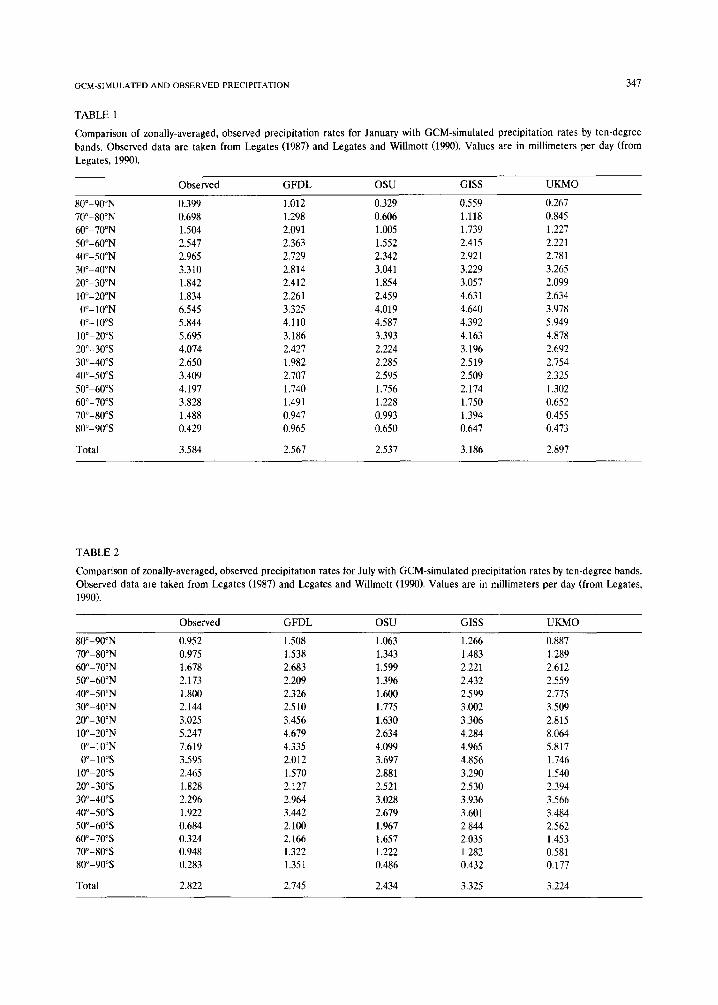
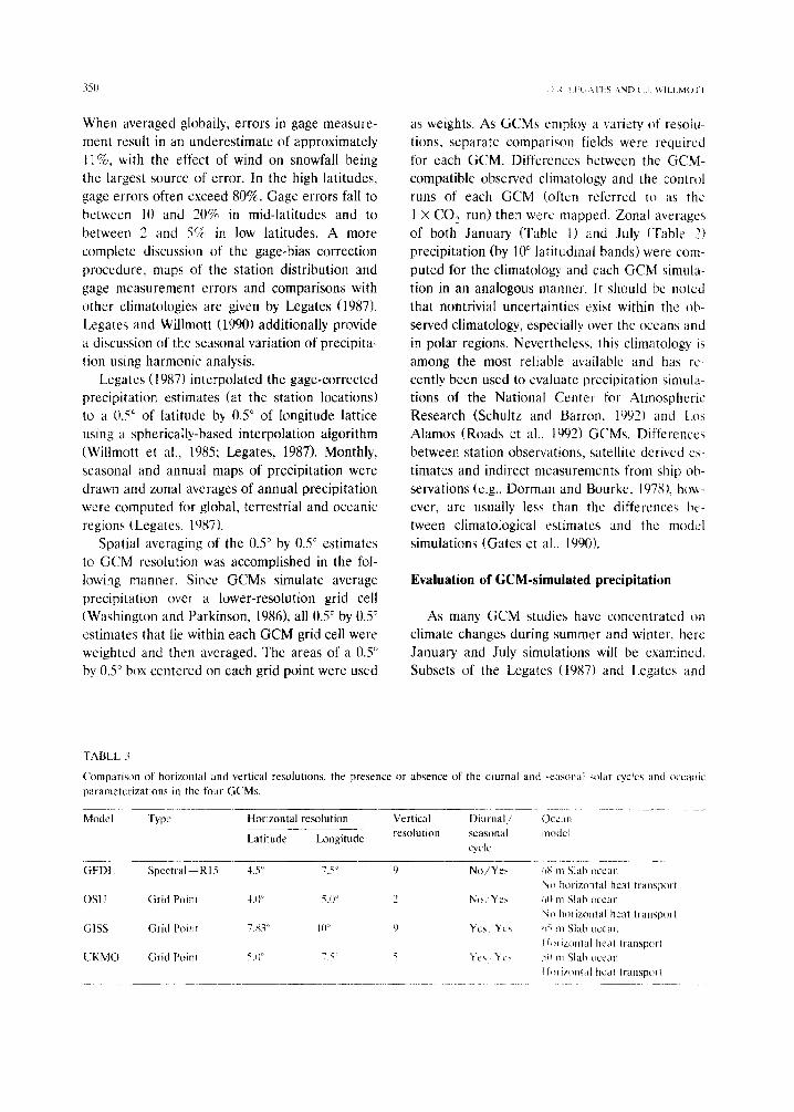
TABLE 1

Comparison of zonally-averaged, observed precipitation rates for January with GCM-simulated precipitation rates by ten-degree bands. Observed data are taken from Legates (1987) and Legates and Willmott (1990). Values are in millimeters per day (from Legates, 1990).

Observed GFDL OSU GISS UKMO

80°-90°N 0.399 1.012 0.329 0.559 0.267 70°-80°N 0.698 1.298 0.606 1.118 0.845 60°-70°N 1.504 2.091 1.005 1.739 1.227 50°-60°N 2.547 2.363 1.552 2.415 2.221 40°-50°N 2.965 2.729 2.342 2.921 2.781 30°-40°N 3.310 2.814 3.041 3.229 3.265 20°-30°N 1.842 2.412 1.854 3.057 2.099 10°-20°N 1.834 2.261 2.459 4.631 2.634 0°-10°N 6.545 3.325 4.019 4.640 3.978 0°-10°S 5.844 4.110 4.587 4.392 5.949

10 °-20°S 5.695 3.186 3.393 4.163 4.878 20°-30°S 4.074 2.427 2.224 3.196 2.692 30°-40°S 2.650 1.982 2.285 2.519 2.754 40°-50°S 3.409 2.707 2.595 2.509 2.325 50°-60°S 4.197 1.740 1.756 2.174 1.302 60°-70°S 3.828 1.491 1.228 1.750 0.652 70°-80°S 1.488 0.947 0.993 1.394 0.455 80°-90°S 0.429 0.965 0.650 0.647 0.473

Total 3.584 2.567 2.537 3.186 2.897

TABLE 2

Comparison of zonally-averaged, observed precipitation rates for July with GCM-simulated precipitation rates by ten-degree bands. Observed data are taken from Legates (1987) and Legates and Willmott (1990). Values are in millimeters per day (from Legates, 1990).

Observed GFDL OSU GISS UKMO

80°-90°N 0.952 1.508 1.063 1.266 0.887 70°-80°N 0.975 1.538 1.343 1.483 1.289 60°-70°N 1.678 2.683 1.599 2.221 2.612 50°-60°N 2.173 2.209 1.396 2.432 2.559 40°-50°N 1.800 2.326 1.600 2.599 2.775 30°-40°N 2.144 2.510 1.775 3.002 3.509 20°-30°N 3.025 3.456 1.630 3.306 2.815 10°-20°N 5.247 4.679 2.634 4.284 8.064 0°-10°N 7.619 4.335 4.099 4.965 5.817 0°-10°S 3.595 2.012 3.697 4.856 1.746

10°-20°S 2.465 1.570 2.881 3.290 1.540 20°-30°S 1.828 2.127 2.521 2.530 2.394 30°-40°S 2.296 2.964 3.028 3.936 3.566 40 °-50°S 1.922 3.442 2.679 3.601 3.484 50°-60°S 0.684 2.100 1.967 2.844 2.562 60°-70°S 0.324 2.166 1.657 2.035 1.453 70°-80°S 0.948 1.322 1.222 1.282 0.581 80°-90°S 0.283 1.351 0.486 0.432 0.177

Total 2.822 2.745 2.434 3.325 3.224

mm

p

er

day

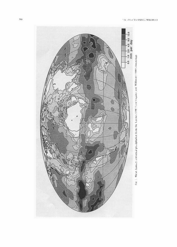
big.

i

Mea

n J

;tnu

ar;

cow

,cot

ed p

reci

pita

ti{)

n tr

om t

he

Leg

ates

(I'

487)

and

L

egat

es a

nd

VV

i]lm

o|l

(]99

(1)

clim

atol

og_~

,

mm

p

er

aa

y

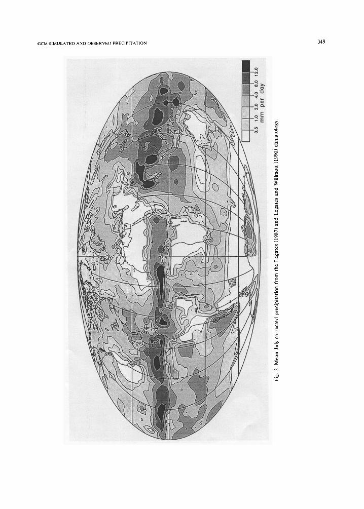
Fig.

2.

Mea

n Ju

ly c

orre

cted

pre

cipi

tati

on f

rom

the

Leg

ates

(19

87)

and

Leg

ates

and

Wil

lmot

t (1

990)

clim

atol

ogy.

35{) I )l'-: I I : G A 1 I S A N I ) ( I WILI_M()I*I

When averaged globally, errors in gage measurement result in an underestimate of approximately 11%, with the effect of wind on snowfall being the largest source of error. In the high latitudes, gage errors often exceed 80%. Gage errors fall to between 10 and 20% in mid-latitudes and to between 2 and 5% in low latitudes. A more complete discussion of the gage-bias correction procedure, maps of the station distribution and gage measurement errors and comparisons with other climatologies are given by Legates (19871. Legates and Willmott (1990) additionally provide a discussion of the seasonal variation of precipitation using harmonic analysis.

Legates (1987) interpolated the gage-corrected precipitation estimates (at the station locations) to a 0.5 ° of latitude by 0.5 ° of longitude lattice using a spherically-based interpolation algorithm (Willmott et al., 1985; Legates, 1987). Monthly, seasonal and annual maps of precipitation were drawn and zonal averages of annual precipitation were computed for global, terrestrial and oceanic regions (Legates, 19871.

Spatial averaging of the 0.5 ° by 0.5 ° estimates to GCM resolution was accomplished in the fol- lowing manner. Since GCMs simulate average precipitation over a lower-resolution grid cell (Washington and Parkinson, 19861, all 0.5 ° by 0.5 ° estimates that lie within each GCM grid cell were weighted and then averaged. The areas of a 0.5 ° by 0.5 ° box centered on each grid point were used

as weights. As GCMs employ a variety of resolutions, separate comparison fields were required for each GCM. Differences between the GCM- compatible observed climatology and the control runs of each GCM (often referred to as the 1 × CO 2 run) then were mapped. Zonal averages of both January (Table I) and July {]'able 2) precipitation (by 10 ° latitudinal bands)were computed for the climatology and each GCM simulation in an analogous manner. It should be noted that nontrivial uncertainties exist within the observed climatology, especially over the oceans and in polar regions. Nevertheless, lhis climatology is among the most reliable available and has re- cently been used to evaluate precipitation simulations of the National Center for Atmospheric Research (Schultz and Barron, 19921 and Los Alamos (Roads et al., 19921 GCMs. Differences between station observations, satellite derived cs- timates and indirect measurements from ship observations (e.g., Dorman and Bourke, 1978), however, are usually less than the differences between climatological estimates and the model simulations (Gates et al.. 19901,

Evaluation of GCM-simulated precipitation

As many GCM studies have concentrated on climate changes during summer and winter, here January and July simulations will be examined. Subsets of the Legates (1987) and Legates and

T A B L E 3

Compar i son of horizontal and vertical resolutions, the presence or absence of

parameter iza t ions in the four GCMs.

the diurnal and seasonal ,,olar cycles and oceatfic

Model Type Horizontal re~)lution Vertical D i u r n a l / Ocean

Lat i tude Longi tude resolution seasonal model cycle

G F D [ . S p e c t r a l - RI5 4.5 ° 7.50 9 N o / Y e s !~S m Slab ocean

No horizontal heat t ranspor t

OSU Grid Point 4.i) ° 5.0 ° 2 N o / Y e s ~it m Slab ocean

No horizontal heat t ranspor t

GISS Grid Point 7.83 ~ 1¢~ '~ 9 Y e s / Y e s ~,'~ m Slab ocean

[Iorizontal heat t ransporl

U K M O (;rid Poml 5.t1" 7 .5 5 '~ es Yes 5(! m Slab ocean

l[oriz~mtai heat t ransport

0 11

1111

IJ

l~l

I.Jl

.I ~

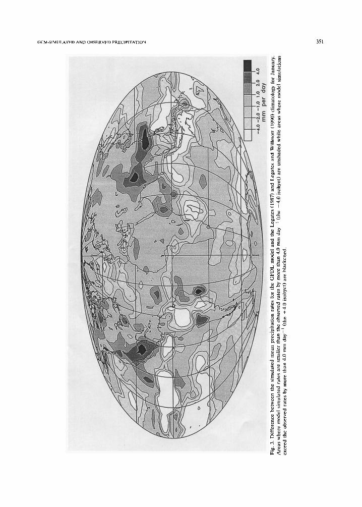
Fig

. 3.

Dif

fere

nce

bet

wee

n t

he

sim

ula

ted

mea

n p

reci

pit

atio

n r

ates

fo

r th

e G

FD

L m

od

el a

nd

th

e L

egat

es (

1987

) an

d L

egat

es a

nd

Wil

lmo

tt (

1990

) cl

imat

olo

gy

fo

r Ja

nu

ary

. A

reas

wh

ere

mo

del

sim

ula

ted

rat

es a

re s

mal

ler

than

th

e o

bse

rved

rat

es b

y m

ore

th

an 4

.0 m

m d

ay-1

(th

e -4

.0 i

soh

yet

) ar

e u

nsh

aded

wh

ile

area

s w

her

e m

od

el s

imu

lati

on

s ex

ceed

th

e o

bse

rved

rat

es b

y m

ore

th

an 4

.0 m

m d

ay

I (t

he

+ 4

.0 i

soh

yet

) ar

e b

lack

ened

.

~N

HJ

pu

t u

uy

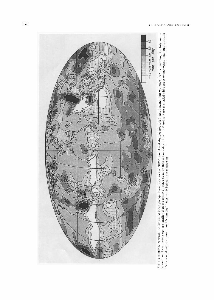
t-ig

~ i

, 1

,1er

ence

bet

v~

een

th

e si

mu

late

d m

ea

n p

reci

pit

atio

n l

ates

fo

r th

e G

FD

L

mo

del

an

ti l

he

Le

ga

tes

(19

87

) an

d L

egat

es a

nd

Wit

lm<

)tt

t 19

9t/)

cli

mat

olo

gy

lo

t .I

ul}.

Are

a,

wh

ere

m~

del

sim

ula

ted

rat

es a

re s

mal

ler

than

th

e o

bse

rve

d r

ates

by

mo

re t

han

4.0

mm

day

~

(th

e 4

.0 i

soh

yet

) :i

re u

nsh

ad

ed

wh

ile

area

s w

he

re m

od

el s

imu

lati

on

s ex

ceed

th

e ~

)bsc

rvcd

rat

es b

~ m

ore

th

an 4

.tlm

m d

a~

(lh

c +

4.(

!iso

hy

et)

are

bla

ck

en

ed


Wiilmott (1990) observed (gage-bias corrected) mean January and July precipitation at 2 ° by 2 ° resolution are shown (Fig. 1 and 2, respectively).

Observed global precipitation is used to evaluate four different GCMs which previously have been used to simulate the climatic effects of increased concentrations of atmospheric Carbon Dioxide. These GCM control runs were chosen because they have been widely used and cited and offer a variety of different resolutions and parameterizations (Table 3). All four model simulations are distributed by the National Center for Atmospheric Research (Jenne, 1988; Joseph, 1989).

Of these four models, the Geophysical Fluid Dynamics Laboratory (GFDL) model (Manabe and Wetherald, 1987) is the only spectrally-based model and uses Rhomboidal truncation at fifteen waves (approximately 4.5 ° of latitude by 7.5 ° of longitude resolution). This model has nine vertical atmospheric layers, a seasonal but no diurnal cycle and a 68 m mixed-layer ocean. It does not, however, include horizontal heat transport (Q- flux). The Oregon State University (OSU-- Schlesinger and Zhao, 1989), the Goddard Insti- tute for Space Studies (GISS--Hansen et al., 1983) and the United Kingdom Meteorological Office (UKMO--Wilson and Mitchell, 1987) grid-point models also are examined. Although it contains only two vertical layers, the OSU model has the highest horizontal resolution of any of the models evaluated here--4 ° of latitude by 5 ° of longitude. The GISS model has nine vertical lev- els and a spatial resolution of 7.83 ° of latitude by 10 ° of longitude. Resolution'of the UKMO GCM is eleven vertical layers and 5 ° of latitude by 7.5 ° of longitude. All three grid-point models use a mixed layer ocean--50 m (UKMO), 60 m (OSU) and 65 m (GISS) deep--although the OSU model does not use the Q-flux method. Both the GISS and UKMO GCMs employ a diurnal solar cycle; the OSU model does not. All four models simulate the complete seasonal cycle.

The GFDL model

In comparison with the observed data, the GFDL model considerably underestimates the

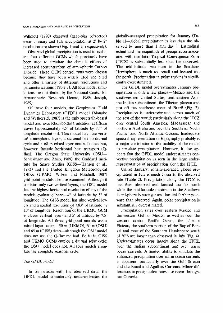
globally-averaged precipitation for January (Ta- ble 1)--global precipitation is less than the observed by more than 1 mm day -1. Latitudinal extent and the magnitude of precipitation associated with the Inter-Tropical Convergence Zone (ITCZ) is substantially less than the observed. The mid-latitude maximum in the Southern Hemisphere is much too small and located too far north. Precipitation in polar regions is signifi- cantly overestimated.

The GFDL model overestimates January precipitation in only a few places--Mexico and the southwestern United States, southeastern Asia, the Indian subcontinent, the Tibetan plateau and just off the southeast coast of Brazil (Fig. 3). Precipitation is underestimated across much of the rest of the world; particularly along the ITCZ over central South America, Madagascar and northern Australia and over the Southern, North Pacific, and North Atlantic Oceans. Inadequate spectral representation of topography probably is a major contributor to the inability of the model to simulate precipitation. However, it also ap- pears that the GFDL model underestimates convective precipitation as seen in the large under- representation of precipitation along the ITCZ.

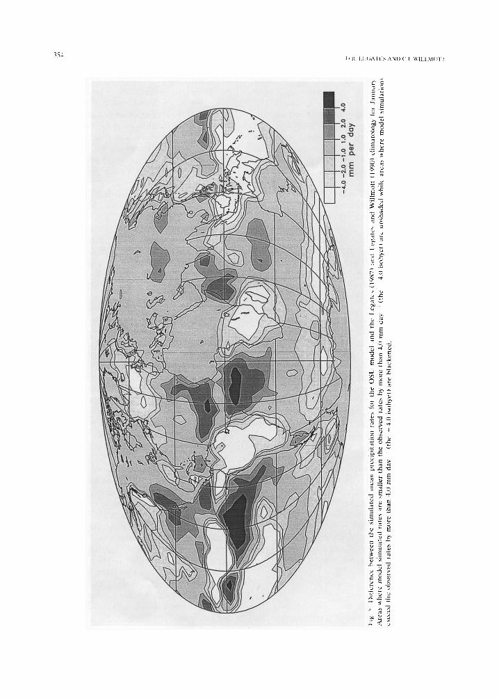
Unlike January, zonally-averaged global precipitation in July is much closer to the observed rate (Table 2). Precipitation along the ITCZ is less than observed and located too far north while the mid-latitude maximum in the Southern Hemisphere is stronger and located farther poleward than observed. Again, polar precipitation is substantially overestimated.

Precipitation rates over eastern Mexico and the western Gulf of Mexico, as well as over the western central Pacific Ocean, the Tibetan Plateau, the southern portion of the Bay of Ben- gal and most of the Southern Hemisphere south of 30°S are larger than observed in July (Fig. 4). Underestimates occur largely along the ITCZ, over the Indian subcontinent and over warm ocean currents. A limited ability to simulate the enhanced precipitation over warm ocean currents is apparent, particularly over the Gulf Stream and the Brazil and Agulhas Currents. Minor differences in precipitation rates also occur throughout Oceania.

mm

p

er

aoy

f:ig

. "~

. D

iffe

ren

ce

hel

wec

n

the

sim

uJa

tcd

me

an

p

reci

pit

atio

n

lare

s to

f th

e O

SU

m

od

el a

nd

th

e L

egat

es (

19

87

) n

nd

l,

egat

e~ ~

md

W~

illm

ott

(19

90

) cl

imat

olo

g),

fo

r ,h

mu

ac~

, A

reas

wh

ere

mo

del

sim

ula

ted

rat

es a

re s

mal

ler

than

th

e o

bse

rved

rat

es b

y m

ore

th

an 4

.0ra

m

day

~

(th

e 4

.0is

oh

yc

t) a

rc

un

sha

de

d w

hil

e ar

eas

~h

erc

m

od

el s

imu

lati

on

~

cx~

'ccd

th

e o

bse

J~cd

[at

es b

y m

~re

th

an

4.0

mm

day

~

(th

e +

4.0

is

oh

yet

) ar

e b

lack

ened

.

Fig

. 6.

Dif

fere

nce

be

twe

cn

th

e si

mu

late

d m

ea

n p

reci

pit

atio

n r

ates

fo

r th

e O

SU

mo

de

l an

d t

he

Le

ga

tes

(19

87

) an

d L

eg

ate

s a

nd

Wil

lmo

tt (

19

90

) cl

imat

olo

gy

fo

r Ju

ly.

Iso

hy

ets

are

- 4.

0,

- 2.

0,

- 1.

0,

1.0,

2.0

an

d 4

.0 m

m d

ay

- i.

Are

as

wh

ere

mo

de

l si

mu

late

d r

ates

are

sm

all

er

than

th

e o

bse

rve

d r

ates

by

mo

re t

han

4.0

mm

day

I

(th

e -

4.0

iso

hy

et)

are

un

sha

de

d w

hil

e ar

eas

wh

ere

mo

de

l si

mu

lati

on

s ex

cced

th

e o

bse

rved

rat

es b

y m

ore

th

an 4

.0 m

m d

ay

-1

(th

e +

4.0

iso

hy

et)

are

bla

cken

ed.

K 7~

r~

>

Z

©

7~

< r~

.4

> 5 z

J~J

0 H

H,~

IJ

~f

~u

y

t-~

i)

ltlc

rel~

ce

bel

~ee

~!

the

~im

uia

ted

me

an

p

reci

pii

atio

n

rate

~,

for

the

GIS

S m

od

el

and

th

e L

cgat

~',,

~ 9

87

) an

d

i.e~

a~c,

~f~

,.] ~

\'ii

lmo

ll

~199

i)}

~ii

mat

olo

g}

to

~ Ja

nu~

r;~

,\

lt.'d

'~ v

~hc

ic

ii}(}

dc}

~illl

LlJ~

llcd

lT,.i

[cs

al~.

.' S

llla

llel

' [h

illl

lh

c c)

h~,~

lvcc

I la

tey

b~

I}I

Ot'C

th

an 4

.0 m

m d

ay

(th

e -4

.0

iso

hy

cI)

are

un~

;ha(

|e(l

w

hil

e ar

ea~

v~h

~_'r~

: mo

dcl

~iV

ilUl~

i[iO

ll'-

~'×

cecd

th

e ob

scr~

,'cd

rate

s b}

mo

re t

hal~

4.

0 m

m d

a}

(lh

c +

4.0

is

oh

yct

) ar

c b

lack

ened

.

GCM-SIMULATED AND OBSERVED PRECIPITATION 35"7

The OSU model

In January, the OSU model underestimates the observed global precipitation rate by more than 1 mm day-1 (Table 1). As with the GFDL simulation, precipitation along the ITCZ is underestimated in both latitudinal extent and magnitude. The Northern Hemisphere subtropical deserts and the mid-latitude maximum (between 30°N and 40°N), however, are well simulated. Nevertheless, precipitation rates between 40°N and 70°N are less than observed. In the Southern Hemisphere, precipitation rates are considerably underestimated. Subtropical deserts extend too far north and the mid-latitude maximum (between 40°S and 70°S) are underestimated by as much as a factor of three. Precipitation in polar regions of both hemispheres (poleward of 70°N and S) is much better simulated than by the spectral model.

January precipitation is overestimated over the equatorial South Pacific and North and South Atlantic Oceans as well as over the southwest portion of North America, central Asia and the Indian Ocean just south of the Arabian Sea (Fig. 5). It is underestimated along the ITCZ and over south-central and southeastern Africa as well as over much of South America, northwestern North America, the lower Mississippi Valley region and much of the Southern, South Pacific and North Atlantic Oceans. As the OSU model has the highest horizontal resolution of the four models discussed here, many topographically-induced errors are not exhibited by the OSU GCM. Schultz and Barron (1992), in an evaluation of the NCAR CCM1, also found that errors caused by topography decreased as spectral resolution was enhanced.

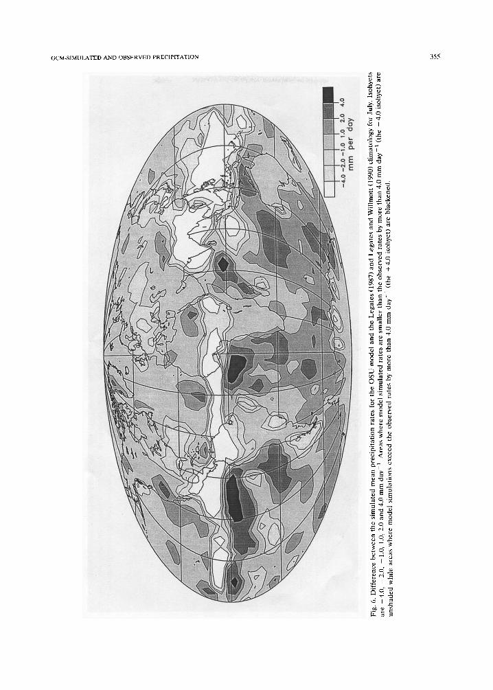
Globally-averaged precipitation rates also are underestimated, albeit slightly, in July (Table 2). Equatorial precipitation again is underestimated and does not extend as far north as the observed. The mid-latitude maximum in the Northern Hemisphere is weaker than observed and, oddly, two maxima are simulated--one between 30°N and 40°N and another between 60°N and 70°N. In the mid-latitudes of the Southern Hemisphere, precipitation rates generally are overestimated

although the mid-latitude maximum is correctly located. Polar precipitation again is well represented.

The OSU model overestimates precipitation rates in oceanic areas just south of the ITCZ, in the southwest of the US and over much of the eastern portions of the oceanic areas of the Southern Hemisphere (Fig. 6). Precipitation rates are less than observed along the ITCZ but also over much of Europe, Japan and East Asia, the southeastern US, eastern Brazil and Uruguay. Once again, these underestimated areas are char- acterized primarily by convective precipitation. Underestimates along and just offshore of the Chilean Andes probably are induced by the inadequate representation of the Andes.

The GISS model

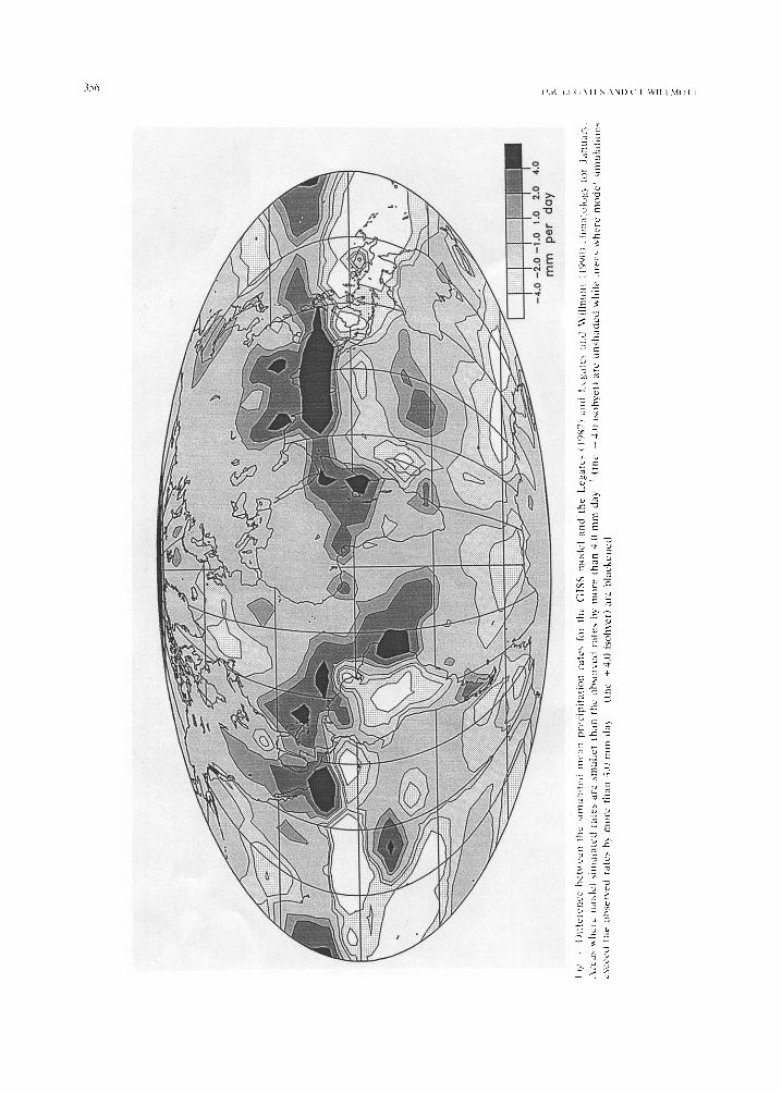
Globally-averaged January precipitation as simulated by the GISS model is closer to the observed precipitation rate than the three other GCM simulations (Table 1). As with the other simulations, however, precipitation along the ITCZ is underestimated, although the GISS model locates the equatorial maximum too far north. Mid-latitude precipitation in the Northern Hemisphere is well represented as are precipitation rates in polar regions. The mid-latitude maximum in the Southern Hemisphere, however, is not well simulated by the GISS model and precipitation rates are approximately half the observed rates.

Simulated precipitation for January is underestimated over the ITCZ, the North Atlantic, the central North Pacific, the western South Pacific and over large portions of the Southern Ocean (Fig. 7). Underestimates also occur over Oceania, central South America, across part of the Great Plains of North America and off the east coast of southern Africa. Precipitation is overestimated in Southeast Asia and India, east central Africa, the equatorial North Pacific Ocean, south of Mexico, the southern Mississippi Valley region and off the east coast of North and South America (between 30°N and 30°S). As before, convective precipitation along the ITCZ is underestimated while precipitation rates are overestimated in the winter

.ji

mm

p

er

day

~-ig

5,.

I)it

lcr,

:ncc

bc

tv, e

e~,

the_

: _~i

mul

atcd

mea

n

prc

cip

itat

itm

~a

tc``

for

til

e (I

tSS

m

od

el

and

the

L

egat

es (

1987

) an

d L

egat

e``

and

Wil

lmo

tt (

1990

) cl

imat

t)lo

gy t

ot

Jul~

A

rea~

~

her

c m

od

el

sim

ula

ted

ra

te',

ar

e sm

alle

r th

an

the

ob

set~

'ed

ra

te``

by

mo

re

than

4.

1) m

m

day

i

(th

e 4.

0 i`

`ohy

et)

are

un

shad

ed

~h

ile

area

`` w

her

e m

od

el

sim

ula

tio

ns

exce

ed

the

ob

serv

ed

rate

s b)

, m

ore

lh

an

4.0

mm

d

a5

I (t

he

+4

.(!

iso

hy

et)

are

bla

cken

ed.

2"

2J

m

)

ITI[H p~r

uu~'

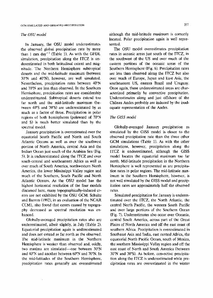
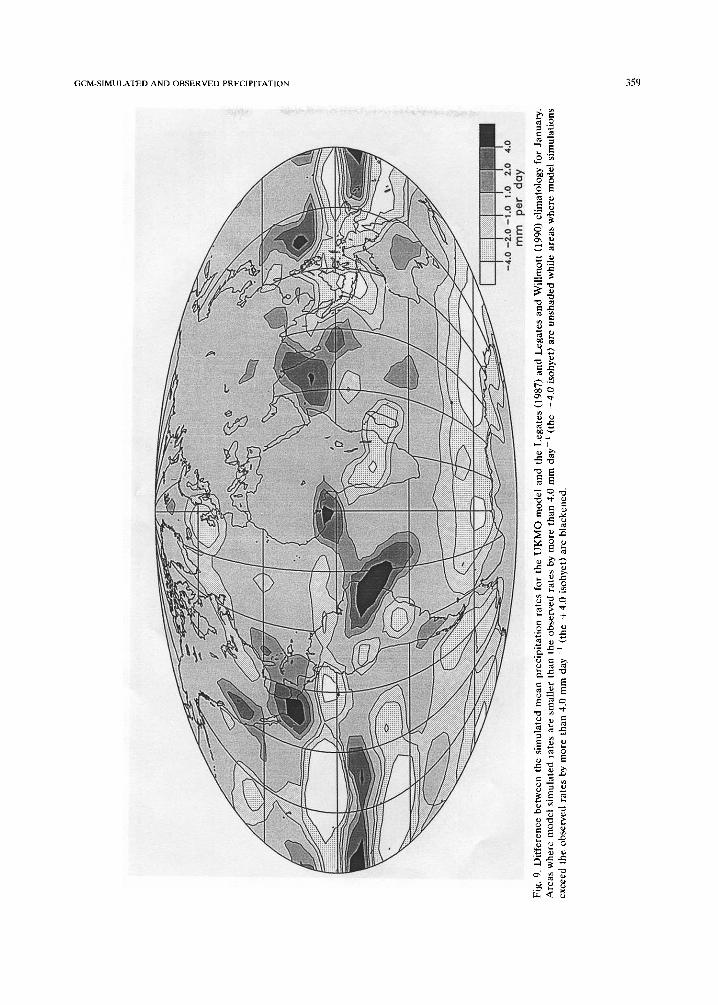
Fig

. 9.

Dif

fere

nce

bet

wee

n t

he s

imu

late

d m

ean

pre

cip

itat

ion

rat

es f

or t

he U

KM

O

mo

del

an

d t

he L

egat

es (

1987

) an

d L

egat

es a

nd

Wil

lmo

tt (

1990

) cl

imat

olo

gy

for

Jan

uary

. A

reas

whe

re m

od

el s

imu

late

d r

ates

are

sm

alle

r th

an t

he

ob

serv

ed r

ates

by

mo

re t

han

4.0

mm

day

1

(th

e -4

.0

isoh

yet)

are

un

shad

ed w

hil

e ar

eas

wh

ere

mo

del

sim

ula

tio

ns

exce

ed t

he o

bse

rved

rat

es b

y m

ore

th

an 4

.0 m

m d

ay-

i (t

he

+ 4.

0 is

ohye

t) a

re b

lack

ened

.

,~,.a

rnm

p

er

day

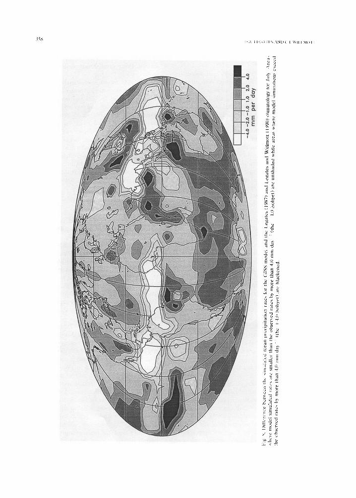
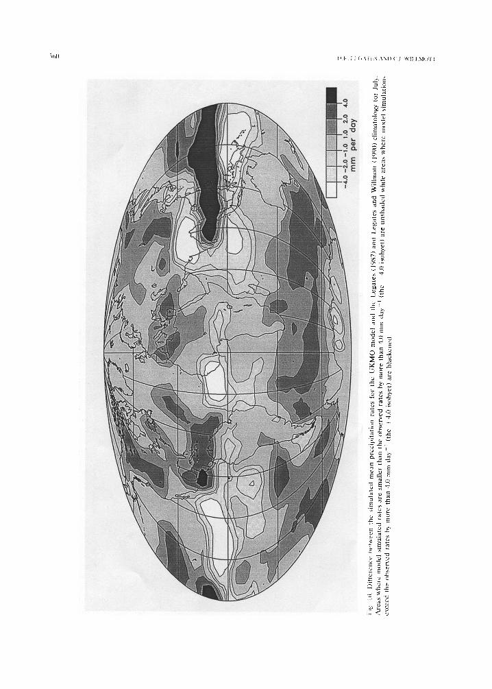
Fig

li~

. l)

irtc

ren

ce

bel

wee

n

tile

si

mu

late

d

mea

n

pre

cip

itat

ion

ra

tes

for

the

UK

MO

m

od

el

and

ti

le

Leg

ates

(19

87)

and

L

egat

es

and

W

illm

ott

(1

9901

cli

mat

olo

gy

for

Ju

b.

Are

as w

her

e m

od

el s

imu

late

d

rate

s ar

e sm

alle

r th

an

the

ob

serv

ed r

ates

by

mo

re t

han

4.0

mm

day

t

(the

4.

0 is

oh

yet

) ar

e u

nsh

aded

w

hile

are

as w

her

e m

~d

el

sim

ula

tio

ns

exce

ed

the

~b

serv

ed

rate

sb}

m

ore

th

an 4

.0 m

m

day

t

(the

+

4.0

iso

hy

et)a

re

bla

cken

ed,


monsoonal areas of the Northern Hemisphere and northward into the Tibetan Plateau. Precipi- tation is well simulated, however, across North- ern Africa, the Middle East, Europe and much of Northern Asia and Australia.

July precipitation is overestimated by the GISS model by more than 0.5 mm day -1 (Table 2). Precipitation rates along the ITCZ are underestimated and the equatorial maximum of precipitation extends too far south. The mid-latitude maximum is overestimated in the Southern Hemi- sphere while the maximum does not appear in the Northern Hemisphere because subtropical precipitation is too great. As with the OSU simulation, precipitation rates poleward of 70°N and S are simulated reasonably well although they are slightly higher than observed.

July precipitation is overestimated across much of the oceanic areas of the Southern Hemisphere (south of 30°S) as well as over the equatorial South Pacific Ocean, eastern Brazil, eastern equatorial Africa and southern India, Indonesia and New Guinea and northeastern Asia (Fig. 8). Underestimates occur along the ITCZ and over much of northern India including the Himalayas. Error patterns similar to those exhibited in Jan- uary occur over North America.

The UKMO model

January latitudinal averages obtained from the UKMO model exhibit the same general trend as those obtained from the OSU GCM although rates simulated by the UKMO model are greater by more than 0.3 mm day-1 (Table 1). Average January precipitation is underestimated, particularly along the ITCZ between 10°N and 20°S. Overall, zonal trends for the rest of the Northern Hemisphere are well-simulated with a correctly located midlatitude maximum. In the Southern Hemisphere, however, precipitation associated with the ITCZ does not extend as far south as the observed and the mid-latitude maximum is not simulated. Precipitation between 40°S and 80°S is considerably underestimated, at times by as much as a factor of six.

January precipitation is overestimated in southern Mexico, southwestern North America,

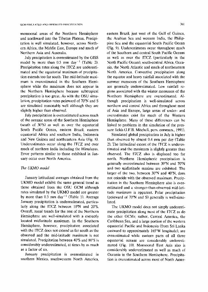
eastern Brazil, just west of the Gulf of Guinea, the Arabian Sea and western India, the Philip- pine Sea and the equatorial South Pacific Ocean (Fig. 9). Underestimates occur throughout much of the Southern and central South Pacific Oceans as well as over the ITCZ (particularly in the North Pacific Ocean), south-central Africa, Ocea- nia, the North Atlantic and much of northeastern North America. Convective precipitation along the equator and heavy rainfall associated with the summer monsoons of the Southern Hemisphere are generally underestimated. Low rainfall regions associated with the winter monsoons of the Northern Hemisphere are overestimated. Al- though precipitation is well-simulated across northern and central Africa and throughout most of Asia and Europe, large areas of under- and overestimates exist for much of the Western Hemisphere. Many of these differences can be linked to problems in the simulation of the pres- sure fields (J.F.B. Mitchell, pers. commun., 1991).

Simulated global precipitation in July is higher than observed by almost 0.4 mm per day (Table 2). The latitudinal extent of the ITCZ is underestimated and the maximum is slightly greater than observed. The ITCZ also is displaced too far north. Northern Hemispheric precipitation is generally overestimated between 30°N and 70°N and two midlatitude maxima are exhibited. The larger of the two, between 30°N and 40°N, does not coincide with the observed maximum. Precip- itation in the Southern Hemisphere also is overestimated and a stronger-than-observed mid-latitude maximum is apparent. Polar precipitation (poleward of 70°N and S) generally is well-simulated.

The UKMO model does not simply underestimate precipitation along most of the ITCZ as do the other GCMs; rather, Central America, the CaribbeanSea, and a large portion of the western equatorial Pacific and Indonesia (from Sri Lanka eastward to approximately 165°W longitude), are overestimated while eastern parts of all three equatorial oceans are considerably underestimated (Fig. 10). Monsoonal East Asia also is considerably underestimated as well as much of Oceania in the Southern Hemisphere. Precipita- tion is overestimated across most of North Amer-

362 ) },~ i [ ( } A i l ! S A N I ) ( " I W l l I . M ( ) I ' I '

ica, southern Europe, northern Africa, the Near East, northeast and central Asia and most of the oceanic areas in the mid-latitudes of the South- ern Hemisphere.

Summary and conclusions

Legates (1987) and Legates and Willmott's (1990) gage-corrected, global precipitation climatology was averaged to the resolution of each of four different climate models (the GFDL, OSU, GISS and UKMO GCMs). Fields for both Jan- uary and July were compared with the GCM- simulated fields. Zonal averages for 10 ° bands of the January and July fields also were computed from the gage-corrected climatology and compared with averages from each of the GCM simulations.

Results indicate that January global precipitation is underestimated by all four GCMs. With the exception of the OSU simulation, a wetter July than January was simulated which is contrary to the observed data. All models generally underestimate precipitation along the ITCZ and underestimate its latitudinal extent. The Southern Hemisphere mid-latitude maximum in January is not adequately simulated by any model and it is underestimated in July. January's maximum may be difficult to simulate because much of the precipitation arises from orographic effects on small land areas between 40°S and 70°S (i.e., extreme southern South America, Tasmania and New Zealand) and over portions of the Southern Ocean which, in the observed climatology, may be artificial. Precipitation in these areas is not adequately simulated due to coarse horizontal model resolution (cf., Schultz and Barron, 1992). North- ern Hemisphere patterns generally are better simulated than their counterparts in the Southern Hemisphere due, in part, to a better topographic representation. Additionally, the GFDL model considerably overestimates polar precipitation (poleward of 70°N and S) as is often characteris- tic of spectral models. Polar precipitation is more adequately represented by the grid-point GCMs (OSU, GISS and UKMO).

Simulated January global precipitation is less than the observed in all four models. This is caused largely by an underestimation of equatorial precipitation and by the absence of the mid- latitude Southern Hemisphere maximum. All models overestimate precipitation to some degrec along the Rockies southward into Central Amer- ica, across eastern Brazil and the South Atlantic, and over India. Precipitation is underestimated in the Southern Ocean, the upper North Atlantic, Madagascar and southeastern Africa and the Pa- cific Northwest of North America, as well as along the ITCZ and across much of South Amer- ica.

July precipitation is better simulated than m January by all four models (cf.. "Fables I and 21 although they tend to overestimate precipitation in oceanic areas of the Southern Hemisphere (south of 30°S), the western North Pacific ocean, and northeastern North America, as well as along the Rocky Mountains. Underestimates occur along the ITCZ and across the Indian subcontinent. Precipitation rates associated with monsoonal areas are inadequately simulated in all models. Summer (wet season) monsoonal precipitation is underestimated by all models while precipitation rates for the winter (dry season) monsoons are often overestimated, particularly by the GISS model and, to a lesser degree, by the GFDL and OSU GCMs. These problems appear to be caused by an inadequate simulation of (1) the latitudinal extent of the ITCZ, (2) its seasonal migration and (3) topography, especially the orographic uplift of the Himalayas. The first two of these problems potentially may be attributable to, or at least accentuated by, the lack of oceanic heat advection in the crudely represented oceans.

As expected, models with higher spatial resolution produce a better simulation of the land/ water dichotomy. All models, however, have trou- ble reproducing the precipitation patterns found in western North America and extreme southern South America, as well as across Monsoon Asia, the Himalayas and the Tibetan Plateau. As regional errors are frequently large (greater than 2 mm day ~), GCM-simulated precipitation should be cautiously used in local and regional studies of climatic change.

GCM-S1MULATED AND OBSERVED PRECIPITATION 363

Acknowledgements

W e would like to t h a n k W.M.L. S p a n g l e r a n d

R.L. J e n n e f rom th e N a t i o n a l C e n t e r for A t m o s -

p h e r i c R e s e a r c h for p rov id ing the c l imate m o d e l

o u t p u t f ields for the four mode ls . He lp fu l com-

m e n t s by J .F.B. Mi tche l l a n d a n o n y m o u s review-

ers are great ly app rec i a t ed . Po r t i ons of th is re-

sea rch we re s u p p o r t e d by N A S A gran t s N A G 5 -

853 a n d N A G W - 1 8 8 4 a n d by N S F g ran t A T M -

9015848.

References

Dorman, C.E. and Bourke, R.H., 1978. A temperature correction for Tucker's ocean rainfall estimates. Quart. J. R. Met. Soc., 104: 765-773.

Eischeid, J.K., Diaz, H.F., Bradley, R.S. and Jones, P.D., 1991. A comprehensive precipitation data set for global land areas. Department of Energy, DOE/ER-69017T-H1, 81 pp.

Gates, W.L., Rowntree, P.R. and Zeng, Q.-C., 1990. Valida- tion of climate models. In: J.T. Houghton, G.J. Jenkins and J.J. Ephraums, (Editors), Climate Change: The IPCC Scientific Assessment. Cambridge Univ. Press, pp. 93-130.

Grotch, S.L. and MacCracken, M.C., 1991. The use of general circulation models to predict regional climatic change. J. Clim., 4: 286-303.

Hansen, J., Lacis, A., Rind, D., Russell, G., Stone, P., Fung, I., Ruedy, R. and Lerner, J., 1983. Climate sensitivity and analysis of feedback mechanisms. In: J. Hansen and T. Takahashi (Editors), Climate Processes and Climate Sen- sivity. Geophys. Monogr. Ser., 29: 130-163.

Hulme, M., 1991. An intercomparison of model and observed global precipitation climatologies. Geophys. Res. Lett., 18 (9): 1715-1718.

Janowiak, J.E. and Arkin, P.A., 1991. Rainfall variations in the tropics during 1986-1989, as estimated from observations of cloud-top temperature. J. Geophys. Res., in press.

Jenne, R., 1988. Data from climate models: The CO 2 warming. National Center for Atmospheric Research, Scientific Computing Division, Data Support Section, 33 pp.

Joseph, D., 1989. Climate model output data. National Center for Atmospheric Research, Scientific Computing Division, Data Support Section, 13 pp.

Kalkstein, L.S. (editor), 1991. Global Comparisons of Selected GCM Control Runs and Observed Climate Data. Environ- mental Protection Agency, Washington, D.C., 251 pp.

Legates, D.R., 1987. A climatology of global precipitation. Publ. Clim., 40(1), 86 pp.

Legates, D.R., 1990. A comparison of GCM-simulated precipitation with a gage-corrected, global climatology: zonal

averages. Proc. Eighth Conf. on Hydrometeorology. Am. Meteorol. Soc., Kananaskis Provincial Park, Alta., pp. 23-28.

Legates, D.R. and Salisbury, J.M., 1990. The effect of measurement errors in precipitation on a hydrologic simulation. Proc., Eighth Conf. on Hydrometeorology. Am. Meteorol. Soc., Kananaskis Provincial Park, Alta., pp. 68-71.

Legates, D.R. and Willmott, C.J., 1990. Mean seasonal and spatial variability in gage-corrected, global precipitation. Int. J. Clim., 10(2): 111-127.

Lockwood, J.G., 1989. Hydrometeorological changes due to increasing atmospheric CO 2 and associated trace gases. Prog. Phys. Geogr., 13(1): 115-127.

Manabe, S. and Wetherald, R.T., 1987. Large-scale changes in soil wetness induced by an increase of atmospheric CO z concentration. J. Atmos. Sci., 44: 1211-1235.

Manabe, S., Wetherald, R.'I. and Stouffer, R.J., 198l. Sum- mer dryness due to an increase of atmospheric CO 2 concentration. Climatic Change, 3: 347-386.

Pitcher, E.J., Malone, R.C., Ramanathan, V., Blackmon, M.L., Puri, K. and Bourke, W., 1983. January and July simulations with a spectral general circulation model. J. Atmos. Sci., 40: 605-630.

Quayle, R.G., 1974. A climatic comparison of ocean weather stations and transient ship records. Mar. Weather Log, 18: 307-311.

Roads, J.O., Chen, S.-C., Kao, J., Langley, D. and Glatzmaier, G., 1992. Global aspects of the Los Alamos general circulation model hydrologic cycle. J. Geophys. Res., submitted.

Schlesinger, M.E. and Zhao, Z., 1989. Seasonal climatic changes induced by doubled CO 2 as simulated by the OSU atmospheric GCM/mixed-layer ocean model. J. Clim., 2(5): 459-495.

Schultz, P. and Barron, E., 1992. Assessment of NCAR general circulation model precipitation in comparison with observations. Palaeogeogr., Palaeoclimatol., Palaeoecol. (Global Planet. Change Sect.), submitted.

Shukla, J. and Mintz, Y., 1982. Influence of land-surface evapotranspiration on the earth's climate. Science, 215: 1498-1500.

Washington, W.M. and Meehl, G.A., 1984. Seasonal cycle experiment on the climate sensitivity due to a doubling of CO 2 with an atmospheric general circulation model cou- pled to a simple mixed-layer ocean model. J. Geophys. Res., 89: 9475-9503.

Washington, W.M. and Parkinson, C.L., 1986. An Introduc- tion to Three-Dimensional Climate Modeling. Univ. Sci. Books, Mill Valley, Calif., 422 pp.

Willmott, C.J., Rowe, C.M. and Philpot, W.D., 1985. Small- scale climate maps: A sensitivity analysis of some common assumptions associated with grid-point interpolation and contouring. Am. Cartogr., 12(1): 5-16.

Wilson, C.A. and Mitchell, J.F.B., 1987. A doubled CO 2 climate sensitivity experiment with a global climate model including a simple ocean. J. Geophys. Res., 92: 13315- 13343.

a comparison of gcm-simulated and observed mean january and july precipitation

Documents