Analytica Chimica Acta, 112 (1979) 11-30 Computer Techniques and Optimization o EIsevier Scientific Publishing Company, Amsterdam - Printed in The Netherlands

A COMPARISON OF FIVE PATTERN RECOGNITION METHODS BASED ON THE CLASSIFICATION RESULTS FROM SIX REAL DATA BASES

MICHAEL SJ&TRBM

Research Group for Chemometrics. Department of Chemistry, UmeB University, S-901 87 Ume& (Sweden)

BRUCE R. KOWALSKI

Laboratory for Chemometrics. Department of Chemistry, University of Washington. Seattle, Washington 98195 (U.S.A.)

(Received 11 August 1978)

SUMMARY

Several pattern recognition methods are compared, including the Bayesian classifica- tion rule, linear discriminant analysis, the K-nearest neighbour rule, the linear learning machine for multicategory data, and soft independent modeliing of class analogy. Several preprocessing methods are discussed in connection with these methods. Six real data bases previously described in the literature are investigated with these methods and the advantages and !imitations of the preprocessing and classification methods are discussed.

Multivariate data analysis in the form of pattern recognition has proved a versatile tool for extracting information from data bases in chemistry [ 1, 2]_ The reasons can be traced to several factors of which the following are con- sidered the most important. First, there is the large amount of data generated by modem spectroscopic methods, data often of multivariate type and from which classification problems can be formulated. Secondly, the comples nature of systems studied in many branches of chemistry is such that models and methods for data interpretation which are applicable to systems of lower complexity, e.g. in physics, are often of little value. Thirdly, suitable program packages for data analysis have been developed where the pattern recognition methods included have been adapted for chemical purposes_

A pattern recognition problem can be formulated in the following way. For N objects, it is known or can be assumed that each object belongs to one of Q classes. An object is characterized by a data vector yi with M elements, where each element in the vector consists of a measurement of a variable_ The objects with known class membership belong to a training set from which information is extracted to permit separation of the classes from

each other. In some applications this information is used to classify a set of T additional objects (a test set) with known data vectors but with unknown class membership (Fig. 1). The possibility that some of the objects in the

12

Fig. l_ Observation matrix for a classification problem.

Fig. 2. A graphical representation of a twoclass problem with three variables.

training set or test sets belong to none of the classes must also be considered in many applications. It shouId be noted that for many classification prob- lems there is no prior information of the variable relevance of the variables

included. In fact, one of the more urgent purposes of a classification approach is to elucidate differences between the classes in the training set and to deter- mine which variables contain information about these differences_

A pattern recognition problem with three variables (M = 3) can be illus- trated by a three’dimensional plot where each object is represented by a point in this space. Figure 2 shows such a visualization of a three-variable problem with two classes. In the same way, each object in a problem where fiZ> 3 can be thought of as a point in an M-dimensional space.

In the literature, technical and computational aspects of pattern recogni- tion methods have been the principal topics discussed_ The performance of a method is often demonstrated by a single example, sometimes only on a synthetic data base and without comparisons with other methods_ These limitations have recently been discussed and emphasized by Kanal [3] _ Con- sequently, it was considered desirable to compare the information that can be gained from a number of real data bases when different preprocessing and classification methods are used.

From pattern recognition problems in the literature, six real data bases were selected for investigation by the following methods: the Bayesian clas- sification rule (BAY ES), linear discriminant analysis (LDA), the K-nearest neighbo_ur rule (KNN), the linear learning machine for multicategory data (LLM), and the soft independent modelling of class analogy (SIMCA). These well-documented methods are probably the most frequently used in chemical applications, and they are easily available through the ARTHUR [4,5], SPSS [6] and SlMCA [7] packages.

13

EXPERIMENTAL

The calculations based on the ARTHUR and SPSS packages were done at the University of Washington Academic Computer Center and the calcula- tions with SIMCA (version SlMCA-2T) at Ume% University Computer Center.

The computational strategies for solving a problem involved: (i) formula- tion of the classification problem; (ii) preprocessing of data by scaling and/or transformation of data and reduction of the dimensionality of the data; (iii) two- or threedimensional graphic representation of the data; (iv) fitting of the original or the preprocessed data to the chosen classification method; (v) interpretation of the results.

PREPROCESSING METHODS

Scaling and transformation of the uariables Often the variances of the variables differ considerably and prior informa-

tion is not available about the relevance of the variables. A reasonable ap- proach to this problem is to give each variable the same weight in the initial stage of the analysis. This is done by so-called regularization or autoscaling of the variables, so that they all have unit variance and zero mean over the whole data set. If the distribution of a variable is skewed, a transformation of the data is recommended to give a distribution closer to the normal dis- tribution- The scaling and transformation of the data influence the classifica- tion results in different ways for different methods. Three of the methods used - BAYES, LDA and LLM - are not affected by autoscaling.

Variable or feature reduction The exclusion of data which contain little or no class-separating informa-

tion is often crucial for a successful classification. One approach to this problem is to generate from the original M-space (M variables) a new ortho- gonal M-space by solving the eigenvalue problem Rv, = X,, v, , where X, are the eigenvalues, and vm the eigenvectors of R, the correlation matrix A reduction of the dirnensionality of the data can then easily be accomplished by exclusion of the eigenvectors corresponding to the a smallest eigenvalues (eigenvector reduction) and a new (M-a) space is obtained.

Another solution is the SELECT method [ 81. This preprocessing method first selects the most discriminating variable (feature), where the Fisher weight or variance weight can be chosen as the discriminating criterion. This corresponds to finding the variable (feature) which differs the most between the classes in terms of a standardized average. The remaining variables are then decorrelated from the first chosen and reweighted, and the feature which in this step gets the highest weight is chosen as the second feature. Features are selected until a previously specified number of features are selected or a predetermined weight is reached. The method gives orthogonal features where the first remains a single variable, while the others are com- binations of several variables.

14

For LDA in the SPSS program, five stepwise variable selection methods are described based on five different variable reduction criteria (see the SPSS manual [ 6])_ These variable reduction methods were tested here with the inclusion levels P = 0.50 (default values in the SPSS program).

In SIMCA, measures of the discriminating and modelling powers for the variables are given. The initial classification with all variables included is thus usually followed by a re-computation where variables with low dis- criminating and modelling powers are deleted.

The variable reduction methods in the SPSS program have been used only with LDA, and the SIMCA variable reduction method only with SLMCA. The eigenvoctor reduction method and SELECT are used wit‘n BAYES, LLM and KNN.

CLASSIFICATION METHODS

The patteirn recognition methods used are described briefly below, to emphasize the quite different strategies involved in solving problems.

The Bayesian classification For each class, and also over all objects in the training set, the frequency

distribution of each variable is determined [ $91. A probability measure describing the fit of an object to a class can then be estimated from how well the elements of the data vector of the object fit the frequency distributions of the class. The probability for an object is then calculated for each class. The object is then considered to belong to the class with the highest prob- ability_ An orthogonal presentation of the variables is recommended because the method assumes the variables to be independent. As an option in the ARTHUR package [4, 51 the estimated distributions can be smoothed by Gaussian function approximations or by cubic spline functions.

Linear discriminan t analysis For a two-class problem, a class-separating or discriminating function is

determined by a linear combination of the variable vectors yi :

D, = F diYik i= 1

where D, is the discriminating score for object h (Fig. 3). The weights di are determined in such a way that they will exhibit the largest ratio of variances between the two groups relative to that within the groups_ The maximum numbers of discriminating functions L are Q - 1 when the classes are less than or equal to the numbers of variables (Q < M) and M when Q > M.

In the SPSS program, classification information for an object is given as a probability measure of class membership, denoted as P(G/X), where the pooled probability over the classes is unity. The probability measure given, denoted as P(X/G), expresses the probability that an object will be that far a\vay from the discriminant score centroid for a class.

15

Fig. 3. With LDA the original fiZ-space is reduced to an L-dimensional space where L is the number of discriminating functions. Objects with different signs on their scores on the discriminant function belong to different classes. For a two-class problem as in this case.

L = 1. The class centroids are denoted by 0.

Fig. 4. With LLM the classes are separated by an &f - 1 dimensional hyperplane.

Linear learning machine for multicategory data With this method (Q - 1) hyperplanes with the dimensionality M - 1 are

determined by a feedback procedure in such a way that the objects for different classes in the training set fall, as far as possible, on different sides of the hyperplanes [lo] (Fig. 4)_ The method always gives complete sepam- tion of the classes in the training set if the number of variables is larger than the number of objects, whether or not the variables contain class-separating information. This limitation has recently been discussed [ll] . In brief, for a two-class problem, the number of variables (or features) should be less than one fourth of the number of objects in the training set for small data sets (n < 20), and less than one third of this number for larger data sets to pre- vent doubtful classifications.

K-nearest neigh bour rule In the M-dimensional space, the class membership of the K closest neigh-

bours to an object are determined. Normally, the Euclidian distance is used as a measure of the closeness of the objects, although other measurements of distance are also available. An object is then assigned to the class to which the majority of its K closest neighbours belongs [ 121 (Fig. 5). In the KNN routine in the ARTHUR program, the K = 1,3.. -10 closest neighbours are calculated for each object. The training set can then be used to determine the K value giving the best prediction of the training set. In the same way as in the training set, a test-set object is classified in the class to which most of its K closest neighbours belong. This method is heavily dependent on the scaling of the variables, when distances are used as criteria of similarity. In

16

Fig. 5. In KNN the class membership of an object is determined by the majority class membership of its K closest neighbours.

Fig. 6. In SIMCA each class is described by a disjointed PC model. In this case A = 1 for both class 1 and 2 in eqn. (1). An object is considered to show a class-typical behaviour within the volume defined by eqn. (2).

cases where the transformations of the variables are made with the aim of optimizing the separation of the classes in the training set, the same restric- tions of the objects/features ratio are applicable as for LLM. Therefore, for KNN, only those results derived from autoscaled data are presented.

Sitnca A principal component model is fitted to the data y$!) for a class 9 in the training set according to [ 131:

(1)

Consequently each class Q is represented by a disjointed principal-component model characterized by the parameters ~i(4’, fliz’ dependent only on the variables (i = 1,2 . . _ M), and 8 kn (q) dependent only on the objects and where E::’ are the residuals. The number of significant terms A, for a class in eqn. (1) is determined by the so-called cross-validation technique [ 141. The classification of an object p is then accomplished by fitting the data vector of the object to the class model (eqn. 1) with the parameters a?) and pi:’ for the different classes q_ This is followed by comparison of the class residual variances d:) obtained for the object with the typical residuaLvariances S$,“’ for each class by means of F-tests:

F = dE’*/SbqP)* (M-A, and (IV, -A, -l)(M-AA,) degrees of freedom) (2)

17

The object then belongs to the class for which the smallest F value is ob- tained. If an object p, when fitted to a class model, gets 0, values outside the normal rage, i.e. outside OWL, then the distance d?’ is calculated instead as the distance between the OFi, and the object p. (For how ezi,, is defined and for further details, see [15])_ This means that the confidence interval for the class will describe a hypervolume in the M-space (Fig. 6).

In addition, for an object to be considered uniquely classified, the ratio of the next smallest residual variance dEj2 and the smallest residual variance dcq) must be larger than a critical F-value:

P

F = d;)2/$7)2 (M -_A r and M-A, degrees of freedom) (3)

Measures of the modelling as well as the discriminating powers for the variables are also calculated [ 151. SIMCA does not disregard the possibility that an object can belong to none of the classes, or the possibility that an object can belong to more than one class.

DATA BASES

The data bases were chosen to be representative of a large variety of chemical problems. Data bases with few classes and a data base with as many as 40 classes were selected. Classification problems with a few objects in each class, as well as problems with a larger number of objects in the classes, are presented. Problems with few, as well as numerous, variables compared with the number of objects in the training set are also included. Only complete data bases with continuous variables (no missing data) are used. The data bases and the classification problems formulated from them are described briefly below; extensive presentations are available in the cited literature_

Trace element composition of archeological artifacts (ARCH) On 45 obsidian quarry samples known to come from four different

quarries north of San Francisco, ten trace elements were measured. In addition, these measurements were made on 29 obsidian artifacts for which little information of their origin was available. The aim of an earlier pattern recognition approach [16] was to establish to which of the four classes these unknown objects belonged, if any. Consequently, the objects from each of the well-known locations formed the training set with four classes, and the unclassified objects formed a test set.

Cis and tram a, p-unsaturated carbonyl compounds (CARBONYL) Ketones and aldehydes with olefinic double bonds in (Y, &position can

exist in planar cis or trans conformers. For sterically hindered compounds, twisted conformers are also possible. The training set for this data base consists of one class with seven sterically hindered compounds and one class

18

of six trans compounds. The seven measured variables are the frequencies for two i-r_ and two U.V. absorption bands, and the absorption intensities of three of these bands. The test set contains three compounds known to be cis, and twelve compounds with unknown class membership. For seven of these, two different assignments are given. The classification problem was formulated to establish if there were any difference between the two classes, and to which classes the test-set objects belonged. A classification of the three cis com- pounds in the test set in the class with sterically hindered compounds is strong evidence that this class consists of cis compounds. The data were taken from Mecke and Noack [17] and the editing of the data and the formulation of the classification problem from Wold and Sjostrom [18].

Trace element study of blood samples from welders (WELDERS)

Concentrations of 17 trace elements in blood samples from welders [ 191 were measured by spark-source mass spectrometry. The blood samples were divided in four classes with 23,7,28 and 23 samples in each class, repre- senting welders using four different welding techniques. A fifth class was formed by a control group of 68 persons not involved in welding. Of interest are possible dissimilarities between the blood heavy metal compositions of the different classes and the control group.

Trace element composition of oil spiCls (OIL) This data base consists of 40 classes with 10 objects in each class [203 .

The objects in a class are represented by one oil sample from a special oil -field and 9 different artificial weatherings performed on this oil sample. Originally, 22 trace elements were measured for each object, but actual concentrations of only seven of these are available for all samples, so that only the latter data were used. The aim of the investigation was to determine if the infomlation on the trace element composition could be used to make accurate classifications of oil spills of unknown origin.

Taxonomy of iris species (IRIS) Fisher’s classical iris data [21] are often used for model studies. Thus it

was considered valuable to include this nonchemical classification problem here. Three species of iris form the three classes. For 50 flowers (objects) for each class, there are four measured variables (sepal length and width, petal length and width); 25 objects randomly selected from each class form the test set. This means that 25 objects from each class form the training set and that the test set contains 75 objects. The editing of the data is the same as described earlier [ 131.

‘3C-n.m.r_ spectra of exo and endo substituted norbornanes (NMR) This classification problem concerns 13C-n.m.r. spectra of eight exe and

seven endo Bsubstituted norbomanes, where the exo compounds form one

19

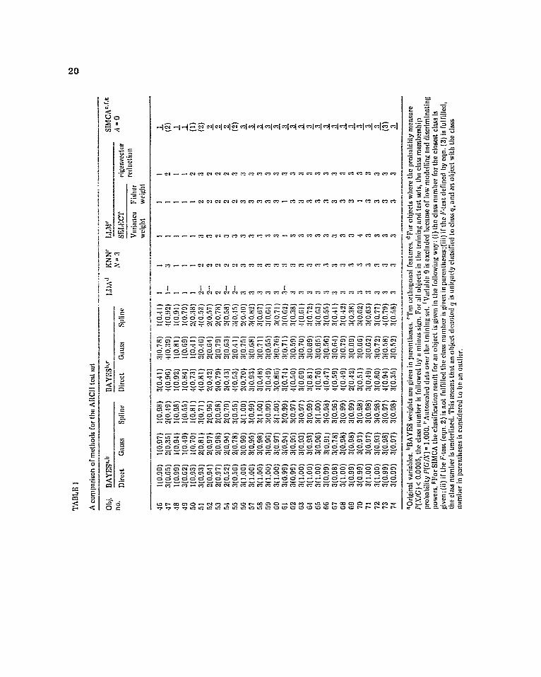
class and the endo compounds another class [ 221. The variables are the seven relative shift differences between the actual structure and the unsubstituted norbomane. In addition, the data base consists of a test set of 28 exe and endo compounds which are, from a chemist’s point of view, related to the compounds in the training set. For all the investigated compounds, it is known which compounds are exe and which are endo. Thus the aim of the pattern recognition approach was not an exo/endo classification but merely to establish: (a) if i3C-n.m.r. shifts contain information on whether a com- pound is an exe or endo compound; (b) which variables (carbon atoms in the molecular framework) contain such information; (c) if the 13C-n.m.r. shifts for the compounds show a behaviour analogous to that of the training set; (d) if a classification approach could give indications of erroneous assign- ments.

RESULTS

ARCH For the training set, all methods solved this classification problem with a

100% correct classification. In contrast, the 29 objects in the test set showed a considerable scatter in the classification from one method to another. The classifications of the test set for the different methods are collected in Table 1. For BAYES and LLM some different preprocessing approaches are also presented. For BAYES the classification is given with and without orthogonalization and with spline and gauss smoothing of the histograms. In the use of LLM a reduction to three features has to precede the classification, since there are few objects in three of the classes. This feature reduction is done with SELECT and with eigenvector reduction.

For all BAYES calculations, the training set is 100% correctly classified. This means that there are no criteria for a preference for one BAYES approach over another, which causes a real dilemma in the test set, when 14 out of 29 objects are not consistently classified. The same problem is present for the LLM calculations where the training set is 100% correctly classified, while for the 29 objects in the test set the classification results differ for 8 objects in the three calculations_ In contrast, LDA, SIMCA and KNN showed very similar classification results; only object 47 is classified differently by these three methods. With SlMCA some objects are classified as outliers (47, 50,51, 55 and 73)_ According to SIMCA, these outliers are not significantly closer to any particular class, which shows that their class membership in- formation is low, and thus explains the startling scatter in the classifications obtained by the different BAYES and LLM approaches for these objects.

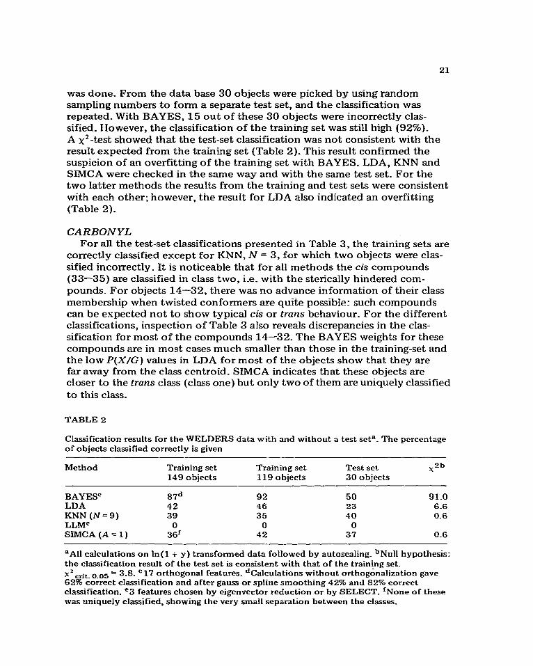
WELDERS For this data base which lacks a test set BAYES gave a superior classifica-

tion (Table 2). This may indicate an over-optimistic number of correctly classified objects. To check for such overfitting, the following experiment

20

21

was done. From the data base 30 objects were picked by using random sampling numbers to form a separate test set, and the classification was repeated_ With BAYES, 15 out of these 30 objects were incorrectly clas- sified. However, the classification of the training set was still high (92%). A x*-test showed that the test-set classification was not consistent with the result expected from the training set (Table 2). This result confirmed the suspicion of an overfitting of the training set with BAYES. LDA, KNN and SIMCA were checked in the same way and with the same test set. For the two latter methods the results from the training and test sets were consistent with each other; however, the result for LDA also indicated an overfitting (Table 2).

CARBONYL For all the test-set classifications presented in Table 3, the training sets are

correctly classified except for KNN, N = 3, for which two objects were clas- sified incorrectly. It is noticeable that for all methods the cis compounds (33-35) are classified in class two, i.e. with the sterically hindered com- pounds_ For objects 14-32, there was no advance information of their class membership when twisted conformers are quite possible: such compounds can be expected not to show typical cis or trans behaviour. For the different classifications, inspection of Table 3 also reveals discrepancies in the clas- sification for most of the compounds 14-32. The BAYES weights for these compounds are in most cases much smaller than those in the training-set and the low P(X/G) values in LDA for most of the objects show that they are far away from the class centroid. SIMCA indicates that these objects are closer to the tram class (class one) but only two of them are uniquely classified to this class.

TABLE 2

Classification results for the WELDERS data with and without a test seta_ The percentage of objects classified correctly is given

Method Training set Training set 149 objects 119 objects

Test set 30 objects

X2b

BAYEF 87d 92 50 91.0 LDA 42 46 23 6.6 KNN (N=9) 39 35 40 0.6 LLM= 0 0 0 SIMCA(A=l) 36’ 42 37 0.6

=A11 calculations on ln( 1 + y) transformed data followed by autoscaling. bNull hypothesis: the classification result of the test set is consistent with that of the training set. x z crit_ o-o5 = 3.8. c17 orthogonal features. dCalculations without orthog&alization gave 62% correct classification and after gauss of spline smoothing 42% and 82% correct classification_ =3 features chosen by eigenvector reduction or by SELECT. ‘None of these was uniquely classified, showing the very small separation between the classes.

22

OIL When the variable distributions were skew, the originally observed y-values

were transformed to In(1 + y) followed by autoscaling. BAYES, LDA, KNN and SIMCA all gave meaningful classifications; SIMCA and BAYES gave the highest rate of correctly classified objects (Table 4). No separation of the

TABLE 3

A method comparison of the test-set classification for the CARBONYL data

Obj. BAYESa BAYESb LDAd KNNe LLhP'f SIhlCXe-h*i

IlO. GZWSC A'=1 IV = 3 Eigenvector SELECT

A = 2 Direct Direct

reduction

14 l(O.96) l(O.51) 15 l(O.79) l(O.52) 16 l(O.99) 2<0.79) 17 l(O.96) l(O.52) 18 2(0.50) 2tO.83) 19 2<0.53) X(0.78) 20 l(O.56) 2<0.83> 21 l(O.54) 2<0.99) 22 1<0.80) 2<0.94) 23 l(O.95) l(O.94) 24 1<0.94) 2w.92) 25 l(O.53) l(O.55) 26 2(0.50) 2(0_76) 27 l(O.99) l(O.95) 28 l(O.99) l(O.52) 29 l(O.53) 2<0.80) 30 1<0_50) l(O.55) 31 1<0_94) l(C.79) 32 1<0_94) l(O.80) 33 2(0.99) 2<0.99) 34 2<0_94) 2<0.99) 35 2(0.99> 2<0.96)

l(O.77) l(O.80) l(O.84) l(O.84) l(O.50) l(O.54) l(O.52) 2(0.57) l(O.79) l(O.71) l(O.79) l(O.58) l(O.79) 1<0.84) l(O.78) l(O.55) 1<0.82) l(O.84) l(0.83) 2tO.65) 2<0.66) 2(0_59)

2- 1 l- l- 2- l- 2- 2- 1 l- l- l- 1 I- 1 l- 1 l- l- 2 2 2

1 1 1 1 1 1 : 1 2 1 1

: 2 2

1 1 1 1 1 1 2 2 I 2 1 1 1 1 2 2 1 2 1 1 1 1 2 2 2 2 2 2

1 1 1 1 1 1 1 1 1 1 1 1 1 1 1 1 1 1 1 2 2 2

1 1 1 1 1 1 2 2 1 1 1 1 1 1 1 1 1 1

: 2 i 2

2 2

(1) 1 i (1) 0 (1) (2) (2) (1) (1) (1) (1) <1) <1) 0 <1) (1) (1) (1) 2

2 (2) -

a? original variables_ b7 orthogonal features_ =Spline approximation gave the same result_ dSee footnote d, Table 1. eAutoscaled data. f2 features_ avariance and Fisher weights gave the same results. h6 variables; variable 3 excluded because of low modelling and discriminating powers. ‘For the presentation of the SIMCA classification, see footnote g, Table l_

TABLE 4

A comparison of the classification results for the OIL dataa

Method Correctly classified objects (%)

BAYESb 92 LDA 88 KNN, N=lC 76 SIMCA (A = 2)d 94

aAll calculations on ln( 1 + y) transformed data. bOrthogonal features. CN = 3, 74% correctly classified. d15% were uniquely classified_ None of the incorrectly classified objects was uniquely classified to another class.

23

classes was obtained with LLM. A comparison of the results from BAYES, LDA and SIMCA classifications with 6, 13 and 8% incorrectly classified objects showed that 20% of all objects were classified incorrectly in at least one of these cases. In addition, when N = 1 and N = 3 in KNN, 24 and 26% of the objects were classified incorrectly. However, 31% of the objects’were classified incorrectly in at least one of these KNN classifications. These results show that the classes overlap partly. This is explicitly indicated by the SIMCA classification where just 15% of the objects were uniquely clas- sified. The small difference in BAY ES weights, and the class membership probability measure P(G/X) in LDA for most objects between the closest and next closest class also reflected this fact.

IRIS All the methods classified class one correctly, and small differences in the

classification of the other two classes were found with only a few objects misclassified (Table 5). For the methods that give some kind of class membership probability measurement (BAYES, LDA and SIMCA), these measures were compared for the objects classified incorrectly in one clas- sification from each of these methods (Table 6). Of these objects, object 134 is classified incorrectly in all three cases. For the other objects classified incorrectly with BAYES, none is classified incorrectly with LDA, and where the class membership probabilities P(G/X) > 0.70. In SIMCA all these objects except object 135 were within the 95% confidence interval for the correct class- The objects classified incorrectly in LDA (except 134) were also clas- sified incorrectly by SIMCA, but not with BAYES. The additional objects classified incorrectly with SIMCA (69 and 132) had high BAYES weights and high class membership probabilities in LDA. Thus for these incorrectly classified objects it is hard to find a major feature in common for the proba- bility measures given for the different methods. However, the BAY ES weights and the P(X/G) values in LDA tend to be lower than the typical values for the objects classified correctly for all methods. It is also noticeable that, among all objects classified incorrectly in BAYES and LDA, none is uniquely classified in SIMCA, a finding that also holds for all objects clas- sified incorrectly in at least one of the classifications presented in Table 5. The SIMCA and LDA classifications are also more similar to each other than to the BAYES classifications_

NMR All methods gave correct classification of the training set with the seven

original variables. In contrast, all methods gave one or more incorrectly classified objects for the test set: objects 21,27,31 and 40-43 were the most frequently misclassified.

For this special problem, SIMCA is attractive because it gives direct in- formation of the variables irrelevant to the classification problem. It also reveals those objects which do not show typical class membership behaidour. For SIMCA, the variables 1-3 and 5 had low discriminating powers [ 22]-

24

TABLE 5

A method comparison for the IBIS data. Objects numbers for incorrectly classified objects are given in parentheses

Method Training set Test set

BAYES= 96%(73,107, 120) 93%(78,127,134,135,139) BAYES= lOO%h 91%(78,88,89,134,139,147,150) KNN,N=3= 97%(107,120) 93%(84,134,135,139,150) LDAd 99%(71) 96%(84,130,134) LLM= 100% 92%(42,126,130,132,134,135) SIMCA (A = 2)= 97%(69,71) 95%(84,130,132,134)

“Autoscaled data. bSpline smoot.hing gave the same results. For gauss smoothing, object 73 is correctly classified but 53 is incorrectly classified. c4 orthogonal features. dCriginal variables_

TABLE 6

A comparison of the class membership probability measures given in a BAYES, a LDA and a SIMCA classification for the IBIS data. Only the objects incorrectly classified in at least one of the classifications are given. The probability measures are underlined for incorrectly classified objects

Obj. no.

BAY ES= LDA= SIMCAb

weights= P(G/X)= P( X/G )d F’(3) Ff(3)

Training set

69 0.80 0.20 7i 0.67 0.35 73 0.50 0.50

107 0.58 0.42 120 0.70 0.30

Test set

78 84

127 130

132

O-72 0.28 0.64 0.36 0.53 0.47 0.99 0.01

1.00 0.00 134 0.51 0.48 135 0.60 0.40 139 O-65 0.35

Typicalg > 0.95 > 0.95 >O.lO <3.2 >20.0

0.96 0.04 0.07 0.57 0.43 0.92 0.08 0.98 0.02 0.36 O-75 0.25 0.02

0.88 0.12 0.73 0.27 0.81 O-19 0.50 0.50 _ 0.99 0.01 0.93 0.07 0.71 0.21 O-74 O-26

0.03 0.11

0.20 0.11 0.15 m 0.25 0.22 0.05 0.09

3.5 3.7 2.6 1.1 0.6 17.0 0.7 8.0

1.6 47 & 1.5 3.5 49 ; 3.3 4.7 4.8 1.5 1.9 2.2

aoriginal variables_ bAutoscaled variables_ CBAYES weights and P(G/X) values (probabili- ties for class membership) for the closest and next closest class. dProbability of the closest object being that distance from the class centroid. ‘=Test for class-typical behaviour (eqn. 2). ‘Test (eqn. 3) showing how close an object is to the model of its next closest class compared with that of its closest class. The F-value is given only if the object is correctly classified_ gTypical values for objects classified correctly for all methods and uniquely in SIMCA.

TABLE 7

A method comparison of the test-set classification for the NMR data

Obj_ no.

Known class

16 1 l(1.00)

17 2 Z(O.96) 18 1 l(1.00) 19 2 2(0.54) 20 1 l(1.00) 21e 2 l( 1.00) 21f 2 l(O.51) 22 1 l(1.00) 23e 2 2(0.96) 23’ 2 2(1.00) 24 1 l(1.00) 25 2 2(0.96) 26 1 l( 1.00) 27 2 l(O.57) 28 1 l(1.00) 29 2 2(0.96) 30 1 l(O.55) 31 2 2(0.98) 32 1 l( 1.00) 33 2 l(O.56) 34 1 l(1.00) 35e 2 35’

2(0.60) 2 2(0.97)

36 1 l(1.00) 37 2 l(O.96) 38 1 1( 1.00) 39 2 2(0.54) 40 1 l(O.96) 41 2 2(0.60) 42 1 l(O.96) 43 2 2(0.61)

BAYEIP KNN= N=l

LDA” LLM= SIMCAC* d A=1

1 2 1 2 1 1 1 1 1 2 1 2 1 1 1 2 1 2 1 2 1 2 2 1 2 1 2 1 2 2 1

l(O.03) 1 2(0.00) 2 l(O.06) 1 2(0.29) 2 l(O.38) 1 l(O.00) 1 l(O.00) 1 l(O.02) 1 2(0.03) 1 2(0.00) 2 l(O.11) 1 2(0.47) 2 l(O.51) 1 l(O.00) 1 l(O.00) 1 2(0.66) 2 l(O.00) 1 l(O.00) 2 l(O.00) 1 l(O.57) 1 2(0.00) 1 l(O.00) 2 2(0.00) 2 2(0.07) 1 l(O.02) 2 l(O.33) 1 2( 0.90) 2 l(O.00) 1 l(O.01) 2 l(O.00) 1 l(O.66) 1

1 2. 1

y - 1

i 2 - 1

i z 1

z i 2 L 2 _A_ 2 1

2 i 2 2

T 2 - 1 - 2

2 2 2

i

aThe three most discriminating features with SELECT after autoscaling. bSeven original variables. The P(G/X) values are given in parentheses_ For all objects the class membership probability P(X/G) = 1.00. With six variables the same poor prediction of the test set was obtained_ =3 variables. dFor an explanation of the presentation of the SIMCA classification, see Table 1 footnote g. eIncorrect assignment_ ‘Correct assignment_

It is illuminating that if only these four lowdiscriminating variables were used in a reclassification, only a 73% correct classification of the training set was obtained; only 20% of the objects were uniquely classified, showing that these variables contained very little class membership information. A classification with the four low discriminating variables excluded gave a 100% classification of the training-set, but in the test-set objects 21, 23,31, 35 and 40-43 were outliers or were classified to the wrong class (Table 7).

26

An examination of the residuals for these objects showed that for the com- pounds 21,23 and 35 the 13C-n.m.r. spectra were not correctly assigned. After a reassignment of these compounds, they were classified correctly 1221. Compound 31 showed large residuals for one of the variables, indicating behaviour inconsistent with the training set. The compounds 40-43 similarly showed large residuals for one of the variables (the shift for the C7 carbon). This special behaviour has been noticed for other compounds which, like compounds 4043, have methyl substituents on the C, carbon [ 23]-

With LDA and with the original seven variables, the misclassifications are numerous in the test set and for most of the objects the P(G/X) values were low (see Table 7). Of the incorrectly assigned objects detected with SIMCA, object 21 was incorrectly and object 23 correctly classified with the incorrect as well as the correct assignments. Object 35 was only correctly classified with the correct assignment. Objects 40-43 were all classified in class 1. The vari- able reduction methods available in LDA were also used and they all excluded variable 7, but no improvement of the test-set classification was thereby obtained.

A feature reduction with SELECT gave (with both variance and Fisher weights) variable ‘7 the highest weight followed by two features mainly derived from variables 6 and 4. These three features were used in a reclassification with BAYES, LLM and KNN. With the different assignments of 21 and 35, LLM classified object 21 in both cases to the incorrect class and 35 to the correct class, thus giving no guide-lines for incorrect assignments_ With BAYES the objects 23 and 35 were classified correctly with incorrect as well as correct assignments. The objects 40-43 were all classified to the correct class. For KNN, N = 1, object 23 was classified incorrectly with incorrect assignment and correctly with correct assignment. For the objects 21 and 35 no con- clusions about their assignments could be drawn.

From these results it is obvious that the far-reaching conclusions drawn from the SIMCA computations are due to an effective variable reduction method, combined with the ability to deal with outliers and to study individual residuak, conclusions that cannot easiIy be drawn from the versions of BAY ES, LDA, KNN and LLM used here_

Feature reduction with SELECT and eigenvector reduction For the classification problems where the classes in the training set are

well-separated, i.e. the ARCH, NMR and CARBONYL data, feature reduction with SELECT or eigenvector reduction can be done with a retained 100% correct classification. For example, for the CARBONYL data a reduction from 7 to 4 or even 2 features with SELECT or eigenvector reduction still gives a 100% correct classification of the training set with BAYES, KNN and LLM.

For problems where the classes are closer to each other in the M-space, resulting in incorrectly classified objects in the training set, e.g. the IRIS, OIL and WELDERS data, no general improvements of the classifications were found after feature reduction. This is exemplified (Table 8) by systematic investigation of the IRIS data.

2f

TABLE 8

Feature reduction of the IBIS data. The percentage of correctly classified objects is given in each case.

BAYES KNN,N=3 LLM

4 orthogonal features 100.93 96.93 2 orthogonal features 92,91 91,92 2 features with SELECT” 97,93b 97,92

100.92 no separation no separation

aVariance weight, no improvement with Fisher weight_ bNo improvement with gauss or spline smoothing of the histograms.

Variable reduction with SIMCA and SPSS When SIMCA was used, all variables contained class-separating information

for the ARCH, OIL and IRIS data. For the WELDERS data all variables showed low discriminating and modelling powers, reflecting the poor infor- mation on class membership contained in this data base_ For the CARBONYL data, only one of the seven variables was excluded (variable 3) and for the NMR data, four of the variables (l-3 and 5) were excluded because of low discriminating powers. The little class-separating information in these was verified in a separate classification with only these four variables.

The variable reduction methods in SPSS used together with LDA gave in just one case a variable reduction on the probability level P = 0.50. This occurred in the NMR data where variable 7 was excluded. This variable is one of the three most discriminating variables according to the SIMCA and SELECT

methods. Instead, variables l-3 and 5, which have low discriminating power according to SIMCA and SELECT, were included.

In LDA, the absolute values of the standardized discriminant coefficient for a variable is a measure of the contribution from the variables to the dis- criminant function [ 51. For example, for the NMR data the variables 34 had the highest coefficients_ Thus these coefficients as a measure of the variable relevance also give a quite different result compared with the SELECT weights and the discriminating powers for the variables given in SIMCA.

Scaling The effects of the scaling of the variables were not systematically investi-

gated. BAYES, LDA and LLM are not affected by autoscaling. Since there were restrictions, such as the limitations on the objects/features ratio when scaling was used to optimize the classification for KNN, it was decided to pre- sent all KNN calculations on autoscaled data. For SIMCA, there are no such restrictions, but the classification results are in most cases retained or improved by autoscaling.

28

Smoothing and orthogonalization in BAYES In no case did smoothing of the histograms and orthogonalization of the

variables give dramatic improvements of the classification results of the training set_ For the classification of the test sets, large discrepancies between different BAYES approaches are prevalent (see, e-g. Tables 1 and 3). But from this investi- gation it is difficult to give any particular approach preference.

DISCUSSION

On the whole, the five pattern recognition methods used performed well. They are well suited to solve classification problems when only classification is of interest and when the classes are well-separated, as in the training-set classification of the NMR, CARBONYL and ARCH data. However, some reservations are in order. BAYES, even if optimal as a classifier when the class distributions are exactly known, seems to be less reliable when used in the way described in this investigation. When the class distributions are unknown, they are estimated from the training set, i.e. the objects to be classified are also used to determine the class distributions. This often leads to an over-optimistic classification of the training set, e.g. for the WELDERS data. Too few objects in the classes lead to poor estimates of the real class distributions, increasing the risk of incorrectly classified objects in the test set. Thus, for chemical applications where the class distributions are rarely known and small data sets are common, BAYES should be used with caution. Application of LDA to the WELDERS data also revealed an over-optimistic test-set classification. However, the overfitting in this case seemed to be less pronounced, as LDA and SIMCA gave a very similar classification of the test sets for the ARCH, CARBONYL and IRIS data.

Futbermore, LLM andLDA should not be used when the ratio of objects to features is less than 3. Another drawback with LLM is that the feedback procedure for the same data set can converge to different hyperplanes [ 24]_

A very poor prediction ability for LLM has also been found by Weisel and Fasching [ 251 using the well known leave-one-out method: one object at a time was excluded from the training set where the objects were 100% correctly classified_ When the excluded objects were treated as test-set objects, only 68% of them were correctly classified_

When the classes are closer to each other, or partly overlap in the M-space, the scatter in the classifications from one method to another can be wide. Thus, to trust the classification results from only a single method in such cases might be inadvisable since the different methods rely on different classification strategies. This dilemma can be partIy circumvented by studying the classifi- cation results from different methods, not with the aim of finding the “best” classification, but with the aim of understanding the data structure and detecting the objects for which the class-separating information is low. The IRIS, OIL and WELDERS data are typical examples where the classes overlap one another and where the methods sometimes give different classification results.

.29

To solve a problem just as a classification problem or as a so-called level-one problem [26] is rarely the sole aim of a chemical pattern recognition method. Of interest in most chemical applications, like the ARCH, CARBONYL and NMR problems, is to obtain information on which objects show atypical class behaviour, i.e. outliers must be considered. This kind of problem (a level- two problem 1261) demands that the method be capable of describing each class as a closed structure in the M-space. Of the methods tested here, only SIMCA fulfils this demand when eqns. (2) and (3) describe each class separately as a closed hypervolume in the M-space. Neither the probability measures P(G/X) and P(X/G) in LDA nor the BAYES weights can describe a closed structure in the M-space. Thus the large discrepancies for the class membership probabilities from method to method found for some of the objects in, e.g., the ARCH, CARBONYL and IRIS data are not surprising. For problems on this level, BAYES, LDA and LLM cannot be recommended when the versions of these methods used are not designed for problems where outliers must be considered. KNN can provide some information of outliers if the actual nearest-neighbours distances of a test-set object are compared with the typical nearest-neighbours distances of the training set, although stringent tests of significance are not described. Also the use of display methods [27] can give some guidance on outliers.

This investigation emphasizes that methods which can deal with outliers are desirable in many chemical applications, since it can rarely be stated in advance that there are no outliers among the objects in the training or test sets. To our knowledge only one method apart from SIMCA, namely the entropy minimax method [ 281, can deal with level-two problems. However, it is probable that some of the existing level-one methods, e.g. KNN, can be further developed as suggested above to deal with outliers.

This work was supported by the Swedish Natural Science Research Council (NFR). M. S. thanks the NFR for a travel grant. We thank Dr. Alice Harper and M. da Koven for helpful discussions.

REFERENCES

1 B. R. Kowalski in C. E. Klopfenstein and C. L. Wilkins (Eds.), Computers in Chemical and Biological Research, Vol. 2, Academic Press, New York, 1974.

2 B. R. Kowalski, Anal. Chem., 47 (1975) 1152A. 3 L. Kanal, IEEE Trans. Inform_ Theory, IT-20 (1974) 697. 4 D. L. Duewer, J. R. Koskinen and B. R. Kowalski, ARTHUR; (available from B. R.

Kowalksi). 5 A. M. Harper, D. L. Duewer and B. R. Kowalski, in B. R. Kowalski (Ed.), Chemometrics,

Theory and Practice, Am. Chem. Sot. Symp. Ser., No. 52,1977. 6 N. H. Nie, C. H. Hull, J. G. Jenkins, K. Steinbrenner and D. H. Brent, SPSS: Statistical

Package for Social Sciences, McGraw-Hill, New York, 1975. 7 S. Weld, SIMCA-2T manual (available from S. Weld). 6 B. R. Kowalski and C. F. Bender, Pattern Recognition, 8 (1976) 1. 9 G. F. Box and G. C. Tiao, Bayesian Interference in Statistical Analysis, Addison-Wesley,

New York, 1973_

30

10 N. B. Nilsson, Learning Machines, McGraw-Hill, New York, 1965. 11 N. A_ B. Gray, Anal. Chem., 48 (1976) 2265_ 12 T. H. Cover and P_ E. Hart, IEEE Trans. Inform. Theory, IT-13 (1967) 21_ 13 S_ Weld, Pattern Recognition, 8 (1976) 127. 14 S. Weld, Technometrics, (1978) in press. 15 S. Weld and M. SjostrSm, in B. R. Kowaiski (Ed.), Chemometrics, Theory and Practice,

Am. Chem. Sot_ Symp. Ser. No. 52,1977. 16 B. R. KowaIski, T. F. Schatzki and F. H. Stross, Anal. Chem., 44 (1972) 2176. 17 R. Mecke and K. Noack, Chem. Ber., 93 (1960) 210_ 18 S. Wold and M. SjGstrijm, in N. B. Chapman and J. Shorter (Eds.), Correlation Analysis

in Chemistry, Pienum Press, New York, 1978. 19 U. Ulfvarsson and S. Weld, Stand. J. Work, Environ. Health, 3 (1977) 183. 20 D. L. Duewer, B. R. Kowaiski and T. F_ Schatzki, Anal. Chem., 47 (1975) 1573. 21 R. A. Fisher, Ann. Eugenetics, 7 (1936) 179. 22 M. SjSstriim and E_ Edlund, J. Magn. Reson., 25 (1977) 285. 23 J. B. Stothers, C. T. Tan and K. C. Teo, J. Magn. Reson., 20 (1975) 570. 24 J. R. McGill and B_ R. Kowalski, J. Chem. Inf. Comp. Sci., 18 (1978) 52. 25 C. P_ Weisel and J. L. Fasching, Anal. Chem., 49 (1977) 2114. 26 C. Aibano, W. Dunn, U. Edlund, E. Johansson, B. Norden, M. SjGstrSm and S. Weld,

Anai. Chim. Acta, 103 (1978) 429. (Computers and Optimization in Anaiyticai Chemistry, Amsterdam, April 1978_)

27 B- R. KowaIski and C. F. Bender, J. Am. Chem. Sot., 95 (1973) 686. 28 A. R. C. Wong and T. S. Liu, IEEE Trans. Comp., 24 (1975) 158.