a comparison of alternative estimators …ageconsearch.umn.edu/bitstream/249685/2/atsedeweyn and...

71

A COMPARISON OF ALTERNATIVE ESTIMATORS OF

MACRO-ECONOMIC MODEL OF ETHIOPIA1

Atsedeweyn A. Asrat2 Olusanya E. Olubusoye3

Abstract

During the past 5 decades a number of econometric techniques were developed and applied to a variety of econometric relationships to deal with the problem of single equation estimation as well as simultaneous equations bias. These days, such methods have very wide applications especially in more developed countries. However, there has been very little attempt to apply these techniques to empirical relationships describing the macro-economic sector of developing countries in general and Ethiopia in particular. In this study, a small macro-econometric model of Ethiopia is used to identify the best estimation techniques that will produce accurate forecast of the economy of Ethiopia. Six econometric methods were considered. The prediction accuracy of these estimators was examined using time series data covering the period 1970 to 2004. The results indicated that considerable gain in forecasting accuracy can be achieved by using 2SLSAUT01 and 2SLSAUT02 than simple ordinary least squares or two stage least squares to estimate macro-economic models.

Key Words: Econometric Techniques, Econometric Models, Ethiopia, Prediction

1 The final version of this article was submitted in July 2008. 2 Asrat Atsedeweyn is Lecturer at the Department of Statistics, University of Gondar, Gondar, Ethiopia. Contact address: [email protected]., Mobile:+251 911 03 96 07. 3 Olusanya E. Olubusoye (PhD) is Assistant professor at the Department of Statistics, University of Ibadan, Ibadan, Oyo State, Nigeria. Contact address: [email protected]., Mobile: +234 805 825 8883

Asrat and Olubusoye: A comparison of alternative estimators of...

72

1. Introduction One of the major challenges that face many African governments is the lack of well-trained Professionals capable of preparing consistent short- to medium-term plans or a comprehensive long-term planning framework. Moreover, over the past years, a number of factors including instability and poor governance have created a time inconsistency problem in policy making in a number of African countries. However, it is expected that the recent trend towards the adoption of poverty reduction strategies that are consistent with overall macro-economic plans will require professionals who can develop and/or use short to longer-term planning frameworks adapted to their economies. Building and updating macro-econometric models require forecasting and planning experts, particularly in the ministries of finance, planning and economic development. In addition budgeting and planning exercises require forecasting major macro-economic variables for at least three to five years. Without such forecasts, the preparation of a country’s resource envelope through annual budgets or what is commonly known as ‘Medium Term Expenditure Framework – MTEF’ would be a difficult task. Forecasting models are a crucial planning instrument. We can use an econometric model to describe how an economy works, and predict future growth rates or carry out simulations to determine how much investment is needed in order to achieve the Millennium Development Goals. Recent budgetary practices in most African countries demand forecasting the government resource envelope three to five years ahead. The invariant coefficients of the equations in a macro-econometric model are estimated from observed data with econometric methods. However, the Ministry of Finance and Economic Development of Ethiopia did not use any of these estimation techniques; rather it uses prior information and experience to fix the values of the parameters for forecasting purposes. But, there are more formal ways of estimating the model than by adjusting coefficient terms for forecasting purposes. The purpose of this study, therefore, is to fill this gap of identifying the best estimation techniques that will produce accurate forecast.

2. Macroeconometric modeling in Ethiopia A comprehensive survey of African macro models by Harris in the mid 1980s and other recent reviews (see Alemayehu 2002, Alemayehu and Daniel 2004) show that macro modelling in Africa is still in its infancy (Harris, 1985)4. Although the development of macroeconomic models has reached a stage were a number of models are now being used on regular basis for forecasting purposes, Ethiopia no

4 This section relies on Alemayehu and Daniel (2004).

Ethiopian Journal of Economics, Volume XVIII, No 1, April 2009

73

longer uses its direct planning approach to manage its economy. On the other hand, the government has no other instrument of economic management either. Thus, the government lacks a macro model that could have facilitated macroeconomic policy analysis for a long period of time. This problem was severe when the effects of proposed policies are not tractable by simple reasoning alone. Nowadays, few models are emerging which contribute towards such end, a detail of which is given as under. Asmerom and Kocklaeuner (1985) constructed a supply side macroeconometric model for Ethiopia. As sited in Daniel (2001), the supply side of the model disaggregates GDP by the production sectors: agriculture, other commodities, construction and distributive service and other services. From the expenditure side, the consumption function (for both private and public), sectorial investment functions, export and import functions are specified. The export function is disaggregated in to coffee and non-coffee and imports are also disaggregated in to capital goods, intermediate goods, consumption goods, fuel, and service imports. Savings are disaggregated in to private and public and specified accordingly. Finally, the saving and the trade gap equations, assuming the trade gap is binding, close the model. The model is fairly disaggregated. But the sectorial equations are not interconnected to capture the simultaneity in the system and hence an exogenous shock in one variable would fail to have any impact on the rest of the system. Moreover, because of the absence of price equation, the effect of any disequilibrium between aggregate demand and supply would completely spills-over to the foreign balance and hence it over or under estimates the foreign exchange gap. Lemma (1993) also constructed a macroeconometric model for Ethiopia. As sited in Daniel (2001), the model has 53 equations (of which 14 are behavioural and the rest 39 are identities) with four major blocks: production sector and investment block, foreign trade block, public finance block and the price block. The model is essentially supply driven and has two productive sectors-agriculture and non- agriculture. The agricultural sector is related to the real relative price the farmers receive, the supply of manufactured goods to the farming sector and other exogenous variables like rainfall. The value added in the non-agricultural sector is specified as a function of the level of monetary investment. The aggregate level of investment, in turn, is a function of major source of funding such as government savings, credit from banking system and foreign capital inflow. The foreign trade block contains three export supply functions (private export functions for pulse and hide; and public coffee export functions) and two import demand functions (capital goods import and raw material imports, and consumers good import is assumed exogenous). The government sector consists of two behavioural government revenue functions (direct and indirect taxes revenue function and import tax function) and an identity export tax revenue function.


74

The government current expenditure and export tax rates are treated as policy instruments. Finally, the price block identifies two price equations based on consumer price index (CPI) and industrial sector price deflator. The change in CPI is related to excess domestic demand (a pure monetarist formulation) and rate of inflation for imported goods. Price in the industrial sector follows a mark-up rule and is indexed to the CPI in the structuralist tradition. The model, by large, describes the structural and institutional peculiarities of the Ethiopian economy and its policy-making institutions of the socialist era (post 1974/75). However, a significant part of the data(10 observations out of 18) used for the period of pre-1974/75 which cannot be described by the above explained model due to a clear institutional and structural differences between the two periods. In addition to this, some of the assumptions in which the model rested constrained the wider use of the model. For instance, the exogeneity assumption on government current expenditure and agricultural price is questionable. In the case where the economy is for external shocks such as war, drought and terms of trade fluctuations, the exogeneity assumption on government recurrent expenditure will not be a fair assumption. Moreover, to the extent that peasants in Ethiopia had been marketing a considerable part of their produce (after fulfilling the levied quota by Agricultural Marketing Corporation) in the flexible price market, treating agricultural price as purely exogenous is not acceptable. The exclusion of the monetary sector and the formulation of CPI equation can also stand in the negative side of the model. Above all, the result of the model suffers from simultaneity bias as each equation in the model is estimated by OLS. Daniel (2001) also constructed a macroeconometric model for Ethiopia. The model is set up in aggregate demand and supply framework. The model has 30 equations of which 14 are behavioural and the rest are identities and technical relationships. As sited in Daniel (2001) this model is designed to capture the peculiar structure of the Ethiopian economy such as its supply-constrained nature. Thus, total output is disaggregated into agricultural and non-agricultural (industry, services and other distributional activities) sectors. Moreover, the economy is characterized by a general capacity under utilization, and an attempt is made to capture this phenomenon. On the demand side, private and public consumption and private investment functions are specified. Public investment is assumed to be exogenous. The domestic demand for imports (disaggregated into consumption, intermediate and raw material imports) and foreign demand for export are included on the demand side. The monetary sector comprises a money demand equation and an endogenously money supply equation. The latter is believed to capture the monetization of deficit. Price and the real exchange equations are specified as endogenous in the model.


75

3. The estimators There are various econometric methods with which we may obtain estimates of the parameters of macroeconometric models5. However, we will consider only the most appropriate estimation methods which may be classified in two main groups, single equation and system-equation techniques. As their names indicate, the main difference between these system estimation methods relates to the information content of the estimator. Another important difference is that single equation estimation techniques involve estimation of the stochastic equations one at a time while system estimation methods all the stochastic equations are estimated simultaneously. Six estimators are considered. The “least squares method” is the starting point for econometric methods. Each estimator is first used to estimate the twelve stochastic equations of the model. The reduced form of the model is then solved for each set of estimates, and within-sample predictions (both static and dynamic) of the endogenous variables of the model are generated over the sample period. The estimators are compared in terms of the accuracy of the within-sample predictions. The general model to be estimated is AY + BX = U (1) where Y is an hxT matrix of endogenous variables, X is k x T matrix of predetermined (both exogenous and lagged endogenous) variables, U is an h x T matrix of error terms, and A and B are h x h and h x k coefficient matrices respectively. T is the number of observations. The ith equation of the model will be written as yi = -AiYi – BiXi + ui, (2) i=1, 2, 3… h, where yi is a 1 x T vector of values of yit (at time t=1,…,T), Yi is an hi x T matrix of endogenous variables (other than yi) included in the i-th equation, Xi is a ki x T matrix of predetermined variables included in the i-th equation, ui is a 1 x T vector of error terms, and Ai and Bi are 1 x hi and 1 x ki vectors of coefficients corresponding to the relevant elements of A and B respectively. The error terms in U are assumed to follow a second-order auto-regressive process:6 5 A model is a group of structural equations describing relationships between economic phenomenon. 6 The process in (3) can easily be generalized to higher-order processes, but that will not be done here since only processes up to second order are considered in the empirical work.


76

U = R(1)U-1 + R(2)U-2 + E, (3) where the R matrices are hxh coefficient matrices, E is an hxT matrix of error terms, and the subscripts denote lagged values of the terms of U. The error terms in E are assumed to have zero expected values, to be contemporaneously correlated but not serially correlated, and to be uncorrelated in the limit with the predetermined, lagged predetermined, and lagged endogenous variables. Many estimators could have been considered, but in order to limit the size and cost of this study, the following six estimators were chosen as some of the more important ones to consider. Ordinary least squares (OLS) The first estimator considered was ordinary least squares applied to each equation of (2). Two-stage least squares (2SLS) The second estimator considered was two-stage least squares applied to each equation of (2). Two-stage least squares produce consistent estimates if and only if the error term ui in (2) is not serially correlated or if there is no lagged endogenous variable in X. With a large sample size, all of the variables in X should be used as regressors in the first-stage regression for each equation. In practice, however, it is usually necessary to use only a subset of variables in X as regressors or to use only certain linear combinations of all of the variables in X as regressors. A necessary condition for 2SLS to produce consistent estimates is that the included predetermined variables in the equation being estimated be in the set of regressors. Otherwise there is no guarantee that 2SLS will produce consistent estimates even if the error term is not serially correlated or if there are no lagged endogenous variables among the predetermined variables. For this study, therefore, the variables in Xi were always included in the set of regressors when the ith equation of (2) was estimated by 2SLS. Ordinary least squares plus first-order serial correlation (OLSAUTO1) The third estimator considered accounts for first-order serial correlation of the error term ui in (2), but not for simultaneous-equations bias. The estimator is based on the assumption that the error term in each equation is first-order serially correlated: ui = rii

(1)ui-1 + ei , i=1,2, …,h, (4) which means that R(1) in (3) is assumed to be a diagonal matrix and R(2) in (3) to be zero.


77

Under this assumption, equations (2) and (4) can be combined to yield: yi = rii

(1)yi-1 - AiYi + rii(1)AiYi-1 – BiXi + rii

(1)BiXi-1 + ei , i=1,2,..,h, (5) Ignoring the fact that Yi and ei are correlated, equation (5) is a simple nonlinear equation in the coefficients rii

(1), Ai and Bi and can be estimated by a variety of techniques. Two of the most techniques are the Cochrane-Orcutt iterative technique and the Hildreth-Lu scanning technique, but any standard technique for estimating nonlinear equations can be used. The technique used for this study was the Cochrane-Orcutt technique. This is because Cochrane-Orcutt technique converges to a stationary value (Sargan, 1964). Two-stage least squares plus first-order serial correlation (2SLSAUTO1) The fourth estimator considered is two-stage least squares applied to each equation of (5). This estimator accounts for both first-order serial correlation and simultaneous-equations bias and produces consistent estimates if R(1) is diagonal and R(2) is zero in (3). In this estimator the following variables must be included as regressors in the first stage regressions in order to ensure consistent estimates of equation (5): yi-1, Yi-1, Xi, and Xi-1. For this study, these variables were always included in the set of regressors. Any standard nonlinear technique can be used for the second-stage regression of equation (5), and the technique used in this study was the Cochrane-Orcutt technique. Ordinary least squares plus first- and second-order serial correlation (OLSAUTO2) The fifth estimator considered accounts for first- and second-order serial correlation of the error term ui in (2), but not for simultaneous-equations bias. The estimator is based on the assumption that the error term in each equation is determined as: ui = rii

(1)ui-1 + rii(2)ui-2 + ei , i=1,2, …,h, (6)

which means that R(1) and R(2) in (3) are assumed to be diagonal matrices. Under this assumption, equations (2) and (6) can be combined to yield: yi= rii

(1)yi-1+rii(2)yi-2 -AiYi+rii

(1)AiYi-1 +rii(2)AiYi-2 –BiXi+rii

(1)BiXi-1+rii(2)BiXi-2 +ei, i=1,2,..,h. (7)

Again, ignoring the fact that Yi and ei are correlated, equation (7) is a simple nonlinear equation in the coefficients rii

(1), rii(2), Ai, and Bi, and can be estimated by a

variety of techniques. The Cochrane-Orcutt technique can be extended in an obvious way to the second-order case, and the extended Cochrane-Orcutt technique was the one used in this study. The technique converged quite rapidly in almost all cases.


78

Two-stage least squares plus first-and second-order serial correlation (2SLSAUTO2) The last estimator considered is two-stage least squares applied to each equation of (7). This estimator is an extension of the estimator discussed in (6) to the second-order case and produces consistent estimates if R(1) and R(2) are diagonal in (3). It is easy to show, following the analysis in (6), that the following variables must be included as regressors in the first-stage regressions in order to insure consistent estimates of equation (7): yi-1, yi-2, Yi-1, Yi-2, Xi, Xi-1, and Xi-2. For this study, these variables were always included in the set of regressors. The nonlinear technique used for the second-stage regressions was the extension of the Cochrane-Orcutt technique to the second-order case.

4. Specification of the model The specification of the model in this study was based on Daniel (2001). This model was chosen because of the advantages that it avoids many of the problems observed on other models as mentioned in part II. The model is yearly and consists of thirty equations of which fourteen are structural, seven are identities and the rest are definitions and technical relationships. The fourteen components are private consumption, private investment, tax revenue, government expenditure, export, import of consumers’ goods, intermediate import, agricultural production, non-agricultural production, capacity utilization rate, price, demand for real money balance, money supply and exchange rate. Aggregate Demand Aggregate demand for domestic output is the sum of domestic absorption and the trade balance. Y= A + (X-Z) 1 (8) where A is domestic absorption and X and Z are export and import, respectively. Domestic absorption is in turn the sum of private consumption (C), investment (I) and government expenditure on domestic goods (G). Private Consumption The economic meaning of consumption is the using-up of economic resources so that they are not available in the future. Consumption is specified as a function of income and price: Log RCpt =β10 + β11 Pt + β12 logRCp t-1 + β13 logRYt+ β14 log RYt-1 (9)


79

where RCpt is real private consumption, P t is the price level and RY is real income at a time t=1,…T. Private Investment Investment is defined as spending which is not for current consumption but for future consumption or to increase the capacity to produce in the future. In other words investment is total spending minus consumption. So investment in the macroeconomic sense is spending on factories and machinery, the development of new mines, increase in the herds of cattle, the building of roads, the building up of the national stock of maize, the building up of foreign exchange reserves and so on. It is specified as: LogIpt = β20∆LogRYt + β21 LogIgt+ β22 LogZt + β23 LogPBt (10) Where PBt is level of public debt, Zt is the level of imports; and Igt is the first difference of government capital stock which is public investment expenditure. Government Sector The government sector is modeled from both the revenue and expenditure sides. From the revenue side, tax revenue is modeled as a function of total output and foreign financial flows and the non-tax revenue is assumed to be exogenous. The expenditure function is also explicitly specified to avoid using it as exogenous policy variable. Assuming expenditure as exogenous is not realistic in Ethiopia since the economy is vulnerable to external shocks such as increase in foreign inflation, foreign interest rate, and an increase or decrease in foreign financial flows. Tax Revenue There are many ways of meeting the cost of government services. In a modern economy, taxation is normally by far the most important way of providing resources to the government, but other methods do exist. Tax revenue is defined to be a function of economic activity proxied by GDP (Y), level of foreign trade and foreign capital flow (F). This is given as Log TR = β30 + β31 logRY t + β32log (X+Z) +β33 logF t Where β3i > 0 and i = 1…3, (11) Government Expenditure In the national accounts, government consumption expenditure is defined to include spending by local authorities as well as by the central government, on the provision of services. The national accounting definition of government consumption spending


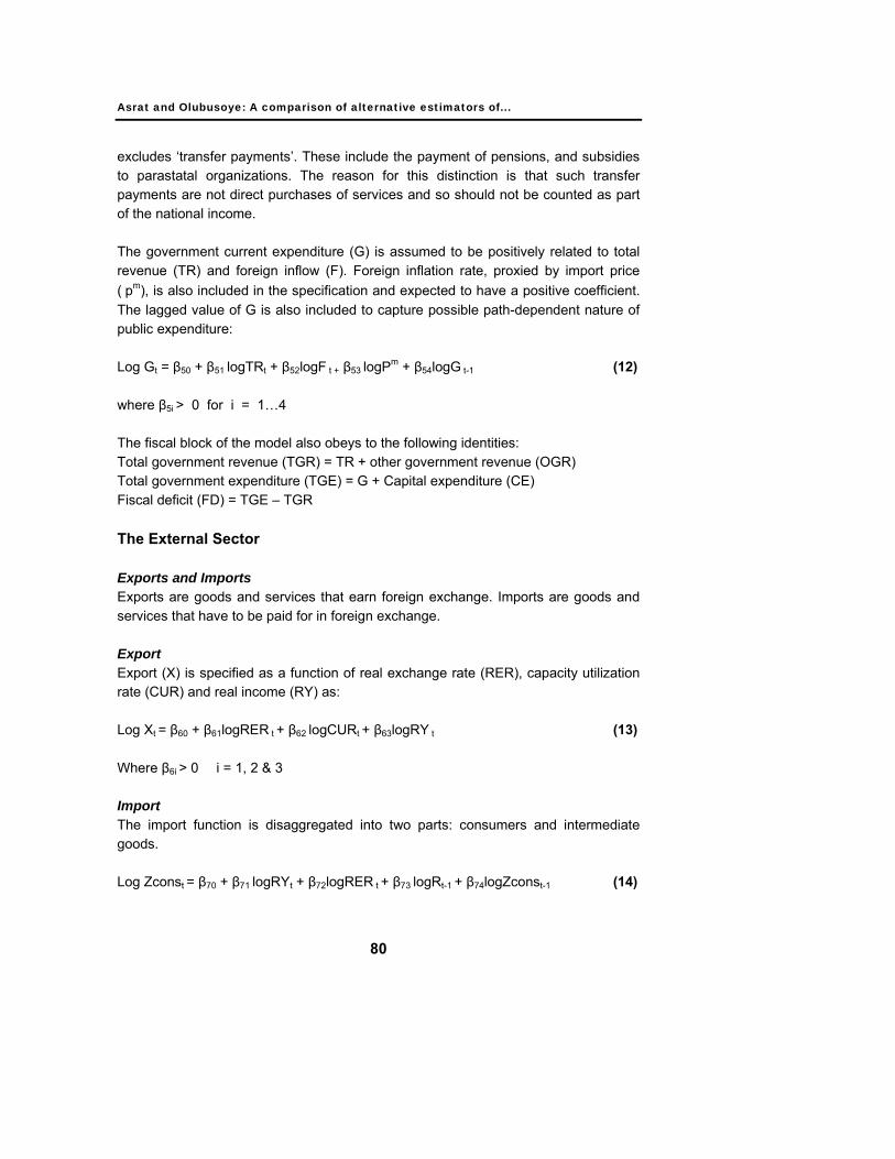
80

excludes ‘transfer payments’. These include the payment of pensions, and subsidies to parastatal organizations. The reason for this distinction is that such transfer payments are not direct purchases of services and so should not be counted as part of the national income. The government current expenditure (G) is assumed to be positively related to total revenue (TR) and foreign inflow (F). Foreign inflation rate, proxied by import price ( pm), is also included in the specification and expected to have a positive coefficient. The lagged value of G is also included to capture possible path-dependent nature of public expenditure: Log Gt = β50 + β51 logTRt + β52logF t + β53 logPm + β54logG t-1 (12) where β5i > 0 for i = 1…4 The fiscal block of the model also obeys to the following identities: Total government revenue (TGR) = TR + other government revenue (OGR) Total government expenditure (TGE) = G + Capital expenditure (CE) Fiscal deficit (FD) = TGE – TGR The External Sector Exports and Imports Exports are goods and services that earn foreign exchange. Imports are goods and services that have to be paid for in foreign exchange. Export Export (X) is specified as a function of real exchange rate (RER), capacity utilization rate (CUR) and real income (RY) as: Log Xt = β60 + β61logRER t + β62 logCURt

+ β63logRY t (13) Where β6i > 0 i = 1, 2 & 3 Import The import function is disaggregated into two parts: consumers and intermediate goods. Log Zconst = β70 + β71 logRYt + β72logRER t + β73 logRt-1

+ β74logZconst-1 (14)


81

where Zcons is import of consumer goods, RYt is real income, RER is real exchange rate and R is total foreign exchange reserves.

log Zract = β80 + β81 logRYt + β82logRER t + β83 logRt-1 + β84logZRact-1 (15)

where Zrac is intermediate import (raw material and capital). In both import equations lagged dependent variables used to show partial stock adjustment behavior. Total import (Z) will then be the sum of consumer, intermediate other imports: Z = Zcons + Zrac + Zother External Sector Closure The external sector is closed by the reserve flows identity in which the accumulation or de-accumulation of reserves take place. Except for the trade balance, the other components of the external sector are exogenous in the model. We will use the identities,

BOP = CA + Transfer payments + capital account balance + net errors and omissions

Change in Reserve = BOP + change in arrears + debt relief

Reserve (t) = Reserve (t-1) + Change in reserve (t) where BOP is the balance of payment and CA (current account) is given as the sum of trade balance + net services + net private transfer payments. Aggregate Supply Total production is disaggregated into agricultural and non-agricultural, the specification of each being informed by stylized facts about the economic structure of the country. Agricultural Production The agricultural production function is assumed to be positively related to labour in the agricultural sector, good rainfall, and relative price of agricultural products. The function is given as:

Log Yagr = β90 + β91 logLagrt + β92logRFt-1 + β93 log(nagr

agr

PP

)t + β94logYagrt-1 (16)


82

Where Yagr is agricultural GDP, Lagr is labour force in agricultural sector7, RF is rainfall, and Pagr/Pnagr is the ratio of agricultural GDP deflator to non agricultural GDP deflator. Non-Agricultural Production The non-agricultural sector refers to both manufacturing and service sectors. Output in this sector is determined by labour, change in capital stock, intermediate import and capacity utilization. This production function is given as Log Ynagr = β100 + β101 log Lnagrt+β102 log∆Kt+β103logZract

+ β104 logCUR (17) Where Lnagr is labour force in non-agricultural sector, ∆Kt is change in capital stock, Zrac is intermediate imports, and CUR is capacity utilization rate in the economy. The total production is given by:

RY= Yagr + Ynagr

Capacity Utilization Rate (CUR) Capacity utilization is defined as actual to potential ratio. It is derived as a ratio of actual GDP to potential GDP. Capacity under utilization may refer to both the agricultural and the non-agricultural sectors. This in the agricultural sector could be due to drought (whose proxy is rainfall). In the non-agricultural sector the main cause of capacity under utilization is shortage of imported inputs. Thus, CUR can be assumed to depend on the level of imports, and rainfall. Log CURt = β110 + β111logRFt-1 +β112logZrac (18)

β i >0 where i = 1 & 2; RF is rain fall and Zrac is intermediate imports. Prices The domestic price level is determined by the real excess demand (RED) over the supply in the domestic economy, excess money supply over the money demand (EMs), and import prices (Pm). In addition, capacity utilization rate (CUR) is also related to the rate of inflation which in turn is related to a mark-up pricing system common in many African industries. Thus, price is specified as: Pt = β120 + β121 EMs + β122log REDt + β123 logCURt + β124logPm

(19) 7 The data for labour force is adjusted using the capacity utilization rate in the agricultural sector to proxy employed labour force in the sector since the data for employed labour force is not available.


83

Money Market The money supply equation is partly endogenous from the side of the balance of payments and the fiscal deficit. Following the flow of funds approach, the domestic money supply (Ms) can be given as Ms = (TGR-TGE) - Gs

p + DCp + ∆R (20) where (TGR – TGE) is the budget deficit, Gs

p is net sales of government interest bearing assets to the non-bank private sector, DCp is domestic credit to the private sector, ∆F is change in foreign financial flows, and ∆R is change in foreign exchange reserve. The demand for real money balance (M/P) is positively related to real income (RY) and negatively related with the opportunity cost of holding money, and given as: Log (M/P)t = β140 + β141 logRY t - β142rt + β143 π t + β144log(M /P )t- (21) Where r and π are interest rate and inflation rate, respectively, that are used to proxy the opportunity cost of holding money. Exchange Rate Since the nominal exchange rate had been fixed for long in the country (only being liberalized in the 1990s), we, rather chose to specify the real exchange rate (RER). Log RER = β150 + β151 logTOT t - β152log(OPEN)t + β153 logFt + β154 EMs (22) where TOT is terms of trade, OPEN = [(X+Z)/ Y] is the trade (export, X, & Import, Z) to GDP, Y, ratio; F is foreign financial flows, and EMs is excess money supply, measured as the difference between money supply and money demand. Identities of the Model

∆LogRY = LogRY - LogRY(-1) RAD = RCp + RCONSg + RIp + RIg RED = RAD - RY FD = G + Ig - TR - NTR TB = X – Z INFLATION = LogP - LogP(-1)

100xPPTOT

Z

X=


84

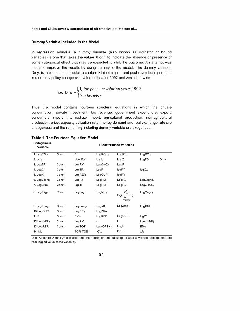
Dummy Variable Included in the Model In regression analysis, a dummy variable (also known as indicator or bound variables) is one that takes the values 0 or 1 to indicate the absence or presence of some categorical effect that may be expected to shift the outcome. An attempt was made to improve the results by using dummy to the model. The dummy variable, Dmy, is included in the model to capture Ethiopia’s pre- and post-revolutions period. It is a dummy policy change with value unity after 1992 and zero otherwise.

i.e. Dmy = ⎩⎨⎧ −

otherwiseyearsrevolutionpostfor

,01992,,1

Thus the model contains fourteen structural equations in which the private consumption, private investment, tax revenue, government expenditure, export, consumers import, intermediate import, agricultural production, non-agricultural production, price, capacity utilization rate, money demand and real exchange rate are endogenous and the remaining including dummy variable are exogenous. Table 1. The Fourteen Equation Model

Endogenous Variable

Predetermined Variables

1. LogRCp

2. LogIp

3. LogTR

4. LogG

5. LogX

6. LogZcons

7. LogZrac

8. LogYagr

9. LogYnagr

10.LogCUR

11.P

12.Log(M/P)

13.LogRER

14. Ms

Const.

Const.

Const.

Const.

Const.

Const.

Const.

Const.

Const.

Const.

Const.

Const.

P

∆LogRY

LogRY

LogTR

LogRER

LogRY

logRY

LogLagr

LogLnagr

LogRF-1

EMs

LogRY

LogTOT

TGR-TGE

LogRCp-1

LogIg

Log(X+Z)

LogF

LogCUR

LogRER

LogRER

LogRF-1

Log∆K

LogZRac

LogRED

r

Log(OPEN)

-Gsp

LogRY

LogZ

LogF

logPm

logRY

LogR-1

LogR-1

log(nagr

agr

PP

)

LogZrac

LogCUR

Π

LogF

DCp

LogRY-1

LogPB

logG-1

LogZcons-1

LogZRac-1

LogYagr-1

LogCUR

logPm

Long(M/P)-1

EMs

∆R

Dmy

(See Appendix A for symbols used and their definition and subscript -1 after a variable denotes the one year lagged value of the variable).


85

5. Individual equations estimation result This section considers the OLS, the 2SLS, the OLSAUTO1, the 2SLSAUTO1, the OLSAUTO2, and 2SLSAUTO2 estimates of Ethiopian macroeconomic model. Data for these time-series analyses were obtained from various sources. All data represent January-December calendar year and annual time-series extending from 1970 to 2004, giving a total of thirty five observations and thereby provide empirical results to various equations in the model formulated in part three. The length of the sample period is determined by the availability of the relevant data. The basic data used for this study are available from the author on request. Combinations of econometric software packages used for empirical analysis of this study are EViews (version 3.1) and STATA (version 9). After confirming the stationarity of the variables at I(0) and I(1), different estimation techniques are applied to estimate the equations and estimation results of the model are summarized in Appendix C. The basic set of instrumental variables used for the two-stage least squares estimators are presented at the bottom of Appendix B.

6. Within-sample forecasting For each sets of estimates, within-sample predictions of the twelve endogenous variables were generated for the period 1970-2004. Comparison of the estimators is carried out in the context of within-sample predictions. In principle, both within and outside sample (ex-post) forecasts must be used. However, for ex-post forecast to be worth while, the time paths must be reasonable length, about ten sample points as a minimum (Challen and Hagger, 1983). As a result of this long forecast period requirement, the ex-post forecast is not performed. Two error measures were computed for each set of predictions: mean absolute percent error and Theil’s Inequality Coefficient. The mean absolute percent error (MAPE) and Theil’s Inequality coefficient (TIC) and its decompositions bias, variance and covariance proportions for private consumption equation is presented in Table 2 for each set of estimates. Generally, the basic conclusions reached for private consumption results also hold for the remaining variables. Evaluation of the Forecasting Power of the Estimators The accuracy of a forecasting method is determined by analyzing forecast errors experiences. The forecasting performance of the estimators is judged on the basis of the differences between predictions and realizations. The smaller the difference between the predictions and the actual values of the dependent variable is the better the forecasting performance of the estimator. The estimators will be compared in


86

terms of the accuracy of the within-sample predictions. The within-sample forecasting performance of the whole system should be assessed using standard statistical tools such as Root Mean Squared Error, Mean Absolute Error, Mean Absolute Percent Error, and Theil’s Inequality Coefficient. The first two forecast error statistics depend on the scale of the dependent variables; and the remaining two statistics are scale invariant (i.e. unit free). In most instances unit-free measures are preferable (Challen and Hagger, 1983). As a result Theil’s inequality coefficient (TIC) and mean absolute percent error (MAPE) are used in this study. If the forecast is good, the mean absolute percent error and the Theil’s inequality coefficient should be as small as possible. Theil’s Inequality Coefficient (TIC) suggested by H.Theil is a measure of the fit of a forecast (H. Theil, 1996). It ranges between zero and one. When it is equal to zero it indicates that the forecast has a perfect fit. TIC=1 indicates a forecast just as accurate as one of “no change” ( ∆ yt = 0), and a value of TIC greater than one means that the prediction is less accurate than the simple prediction of no change (J. Kmenta, 1986). For all of the equations the results indicate that the Theil’s inequality coefficient is close to zero for 2SLSAUT01 and 2SLSAUT02, implying that the forecast has a good fit in these two estimators than the rest. Theil’s inequality coefficient can be decomposed into Bias, Variance, and Covariance proportions each showing a different source of forecast error: • The bias proportion indicates how far the mean of the forecast is from the mean

of the actual series. • The variance proportion indicates how far the variation of the forecast is from the

variation of the actual series. • The covariance proportion measures the remaining unsystematic forecasting

errors. If the forecast is “good”, the bias and variance proportions should be as small as possible so that most of the bias should be concentrated on the covariance proportions. On the basis of these aforementioned selection and evaluation criteria concluding remarks have been drawn. The results in the forecast evaluation indicate that in most of the equations the conclusions reached from examining the mean absolute percent error results and Theil’s Inequality Coefficient results are the same. The TIC for all equations is below 0.3 and has least value for 2SLSAUT01 and 2SLSAUT02. These figures are in the acceptable range since “TIC less than 0.3 or 0.4 are considered not to be unduly large” (Oshikoya, 1990:101). The results also indicate that the model has small values of the mean absolute percent error, the bias and variance proportions in the 2SLSAUT01 and 2SLSAUT02 than the other estimators, implying a good forecast


87

can be achieved by these two estimators. The bias proportion is less than 1% for 2SLSAUT01 and 2SLSAUT02 in all equations. In most of the equations the variance proportion is well below 10% for 2SLSAUT01 and 2SLSAUT02. The result also shows that the bulk of forecast error is unsystematic and hence captured by the covariance proportion. The model reveals a good feature in terms of mean absolute percent error, Theil’s inequality coefficient and its decompositions for 2SLSAUT01 and 2SLSAUT02 than the other estimators. Higher mean absolute percent error (MAPE) is observed in capacity utilization rate equation, price equation, intermediate import equation, real exchange rate and investment function. This is a common feature for most macroeconometric models in the case of developing countries (Salvatore, 1989). For the MAPE measure in these equations, the OLS & 2SLS estimators continue to perform poorly relative to the others, but for the other four estimators the MAPE results are quite close. The mean absolute percent error and Theil’s Inequality Coefficient for the private consumption variable are presented in Table 2 for each set of estimates. The most striking feature of the mean absolute percent error and Theil’s Inequality Coefficient results is perhaps the increased accuracy obtained from the 2SLSAUT01 and 2SLSAUT02 estimates for the predictions. The result in Table 2 also shows that the two stage least squares estimators perform on average better than their ordinary least squares counterparts, that the AUT01 estimators perform on average better than their no-serial correlation counterparts, and that the AUT02 estimators perform on average better than their AUT01 counterparts: 2SLS is better than OLS, 2SLSAUT01 is better than OLSAUT01, 2SLS02 is always better than OLSAUT02, OLSAUT01 is better than OLS, and 2SLS01 is better than 2SLS. The OLS & 2SLS estimators continue to perform poorly relative to the others, and mean absolute percent error and Theil’s Inequality Coefficient results indicate that 2SLSAUT02 estimator can be considered as dominating all of the rest. Table 2: Forecast Evaluation for Private Consumption

Estimator Mean Absolute Percent Error

Theil’s inequality coefficient

Bias proportion

Varianceproportion

Covariance proportion

OLS

2SLS

OLSAUT01

2SLSAUT01

OLSAUT02

2SLSAUT02

0.179479

0.179465

0.166915

0.158079

0.166888

0.158072

0.001192

0.001092

0.001050

0.000985

0.001050

0.000985

0.000020

0.000000

0.000000

0.000000

0.000000

0.000000

0.021872

0.021733

0.020479

0.020001

0.017665

0.017655

0.978108

0.978267

0.979521

0.979999

0.982335

0.982345


88

7. Conclusions This research work is an attempt to select the best and accurate estimator among various estimators which posses high power of predictability (forecasting power). The results in this section indicate that considerable gain in forecasting accuracy can be achieved by the use of more advanced estimation techniques. Certainly, accounting for first- and second-order serial correlation is important, and even more gain appears possible by using a two stage least squares techniques as opposed to its ordinary least squares counterpart. Moreover, the results do indicate that series attempts should be made to estimate models by techniques other than ordinary least squares or two-stage least squares. The results also indicate that considerable gain can be achieved by using 2SLSAUT01 and 2SLSAUT02 estimators. Although a multi-period forecast is not included in this study, the results give an indication of the relative usefulness of the various estimators for multi-period forecasting purposes.

8. Policy implications Based on the finding of this study the following policy implications may be drawn. • The main contribution of this study lies on the application of econometric methods

to identify the best estimation techniques that will produce accurate forecast using macroeconomic model of Ethiopia. Although the model is capable in identifying the best estimation techniques that will produce accurate forecast, the model is in the aggregate form (i.e. further disaggregation is necessary), so it would be more interesting if the model is disaggregated in agricultural, industrial and service sectors. Inclusion of the labor market, disaggregating government expenditures by activities, and disaggregating the production activity in detail would give a better shape for the model. By doing this better performance could be highlighted.

• Technocrats in ministries of finance and economic development have to focus on

the task of macroeconomic forecasting which is of increasing importance in the context of poverty reduction strategies and Medium Term Expenditure Framework-MTEF preparation. In addition to this, strengthening the existing practice of forecasting in Ethiopia is important by providing these technocrats with an applicable framework of modeling that emphasizes forecasting using familiar software such as STATA and EViews. Hence this study will eventually help the policy makers to develop a better understanding of the structure of the economy and how it works. This in turn can result in improved model building as well better policy formulation and forecasting using individual equations techniques and


89

examines how they perform. We may be interested in forecasting the values of some variables either to assess how they respond to given policy changes or evaluate necessary policy responses to a given change in these variables. Generally the output of this research will help the relevant government institutions in designing and revising appropriate techniques for forecasting the economy of the country. Besides its use in budget preparation, policy analysis and simulation exercises, the study provides the foundation for building full-fledged macro model in Ethiopia and as a basis for further research.


90

Reference Alemayehu Geda. 2002. Finance and Trade in Africa: Macroeconomic Response in the World

Economy Context. London: Pallgarve-Macmillan. Alemayehu Geda and Daniel Zerfu. 2004. A Review of Macro Modelling in Ethiopia: With

Lessons form Published African Models. MoFED Working Paper Series, WPs-01, Addis Ababa.

Asemerom Kidane and Kocklaeuner, G. 1985. A Macroeconometric Model for Ethiopia: Specification, Estimation and Forecast and Control. East African Economic Review.

Challen, D. W. and Hagger, A. J. 1983. Macroeconometric Systems: Construction, Validation and Application. London: Macmillan Press.

Daniel Zerfu. 2001. Macroeconomic Policy Modeling for Ethiopia, Unpublished MA Thesis, Department of Economics, Addis Ababa University.

Harris, J. 1985. A Survey of Macroeconomic Modelling in Africa' Paper presented to a meeting of the Eastern and Southern Africa Macroeconomic Research Network, December 7-13, Nairobi, Kenya.

Kementa, J. 1986. Elements of Econometric, second edition, Macmillian, New York. Second edition. Wiley, New York.

Lemma Mered. 1993. Modelling the Ethiopian Economy: Experience and Prospects (memo). Oshikoya, T. W. 1990. The Nigerian Economy: A Macroeconometric and Input-Output Model,

New York: PRAEGER. Salvatore, D. 1989. The Prototype Model, In African Development Prospects: A Policy

Modelling Approach, New York: Taylor and Francis. Sargan, J. D. 1964. Wages and Prices in the United Kingdom: A Study in Econometric

Methodology. Theil, H. 1953. Estimation and Simultaneous Correlation in Complete Equation Systems, The

Hague: Central Plan Bureau.


91

Appendix A : Definition of variables

CUR Capacity utilization rate ∆ Change EMs Excess money supply over money demand, measured as the difference

between money supply and the estimated money supply. F Foreign financial flows (grants + loan and credits) FD Fiscal deficit G Government expenditure Gsp Net sales of government interest bearing assets to the non-bank private sector Ig Nominal government investment ∆K Change in capital stock –i.e gross fixed capital formation Lagr Labour force in agriculture Lnagr Labour in non-agricultural sector Ms Money supply NS Net service export NTR Government non-tax revenue OGR other government revenue OPEN Openness measured as export and imports as a ratio of GDP PB Public borrowing (domestic) Pm Import price Pt Price level measured by the CPI

productturalnonagriculandalagriculturofratioPricePnagrPagr

π Inflation rate r Real deposit interest rate RAD Real aggregate demand RCONSg Real government consumption RCpt Real private consumption expenditure RED Real excess demand RER Real exchange rate RF Rainfall RIg Real government investment expenditure RIpt Real private investment RYt Real output TB Trade balance TGE Total government expenditure TGR Total government revenue TOT Terms of trade TR Government tax revenue X Exports Yagr Agricultural output Ynagr Non-agricultural output Z Total imports Zcons Import of consumers’ good Zothers Other imports (i.e. Z- Zcons –Zrac Zrac Import raw material and capital goods (intermediate imports)


92

Appendix B: Instrumental Variables used for 2SLS in each Equation in addition to those in the basic set Dependent Variables Estimator Instrumental Variables

LogRCp LogIp LogTR LogG LogX LogZcons

2SLS 2SLSAUT01 2SLSAUT02 2SLS 2SLSAUT01 2SLSAUT02 2SLS 2SLSAUT01 2SLSAUT02 2SLS 2SLSAUT01 2SLSAUT02 2SLS 2SLSAUT01 2SLSAUT02 2SLS 2SLSAUT01 2SLSAUT02

LOGIg, LOGRF(-1), LOG∆K, LOGRED, LOGF, LOGPm, LOGR(-1), r, ∆LOGRY, LOGLagr,LOGLnagr,LOGPB,LOGG(-1),LOGZCONS(-1), LOGZrac(-1), LOGYagr(-1), LOGOPEN, FD, NTR, π, TB, RIg, RAD, ∆R, DCp, GS

P. LOGRCp(-1), LOGRF(-1), LOG∆K, LOGRED, LOGRY, LOGF, LOGPm, LOGR(-1), r, LOGLagr, LOGLnagr, LOGRY(-1), LOGG(-1), LOGZCONS(-1), LOGZrac(-1), LOGYagr(-1), LOGOPEN, FD, NTR, π, TB, RIg, RAD, ∆R, DCp, GS

P. LOGRCp(-1), LOGIg, LOGRF(-1), LOG∆K, LOGRED, LOGPm, LOGR(-1), r, ∆LOGRY, LOGLagr, LOGLnagr, LOGRY(-1), LOGPB, LOGG(-1), LOGZCONS(-1), LOGZrac(-1), LOGYagr(-1), LOGOPEN, FD, NTR, π, TB, RIg, RAD, ∆R, DCp, GS

P. LOGRCp(-1), LOGIg, LOGRF(-1), LOG∆K, LOGRED, LOGRY, LOGR(-1), r, ∆LOGRY, LOGLagr, LOGLnagr, LOGRY(-1), LOGPB, LOGZCONS(-1), LOGZrac(-1), LOGYagr(-1), LOGOPEN, FD, NTR, π, TB, RIg, RAD, ∆R, DCp, GS

P. LOGRCp(-1), LOGIg, LOGRF(-1), LOG∆K, LOGRED, LOGF, LOGPm, LOGR(-1), r, ∆LOGRY, LOGLagr, LOGLnagr, LOGRY(-1), LOGPB, LOGG(-1), LOGZCONS(-1), LOGZrac(-1), LOGYagr(-1), LOGOPEN, FD, NTR, π, TB, RIg, RAD, ∆R, DCp, GS

P. LOGRCp(-1), LOGIg, LOGRF(-1), LOG∆K, LOGRED, LOGF, LOGPm, r, ∆LOGRY, LOGLagr, LOGLnagr, LOGRY(-1), LOGPB, LOGG(-1), LOGZCONS(-1), LOGYagr(-1), LOGOPEN, FD, NTR, π, TB, RIg, RAD, ∆R, DCp, GS

P.


93

LogZrac LogYagr LogYnagr LogCUR P LogRER

2SLS 2SLSAUT01 2SLSAUT02 2SLS 2SLSAUT01 2SLSAUT02 2SLS 2SLSAUT01 2SLSAUT02 2SLS 2SLSAUT01 2SLSAUT02 2SLS 2SLSAUT01 2SLSAUT02 2SLS 2SLSAUT01 2SLSAUT02

LOGRCp(-1), LOGIg, LOGRF(-1), LOG∆K, LOGRED, LOGF, LOGPm, r, ∆LOGRY, LOGLagr, LOGLnagr, LOGRY(-1), LOGPB, LOGG(-1), LOGZCONS(-1), LOGYagr(-1), LOGOPEN, FD, NTR, π, TB, RIg, RAD, ∆R, DCp, GS

P. LOGRCp(-1), LOGIg, LOG∆K, LOGRED, LOGRY, LOGF, LOGPm, LOGR(-1), r, ∆LOGRY, LOGLnagr, LOGRY(-1), LOGPB, LOGG(-1), LOGZCONS(-1), LOGZrac(-1), LOGOPEN, FD, NTR, π, TB, RIg, RAD, ∆R, DCp, GS

P. LOGRCp(-1), LOGIg, LOGRF(-1), LOGRED, LOGRY, LOGF, LOGPm, LOGR(-1), r, ∆LOGRY, LOGLagr, LOGRY(-1), LOGPB, LOGG(-1), LOGZCONS(-1), LOGZrac(-1), LOGYagr(-1), LOGOPEN, FD, NTR, π, TB, RIg, RAD, ∆R, DCp, GS

P. LOGRCp(-1), LOGIg, LOG∆K, LOGRED, LOGRY, LOGF, LOGPm, LOGR(-1), r, ∆LOGRY, LOGLagr, LOGLnagr, LOGRY(-1), LOGPB, LOGG(-1), LOGZCONS(-1), LOGZrac(-1), LOGYagr(-1), LOGOPEN, FD, NTR, π, TB, Rig, RAD, ∆R, DCp, GS

P. LOGRCp(-1), LOGIg, LOGRF(-1), LOG∆K, LOGRY, LOGF, LOGR(-1), r, ∆LOGRY, LOGLagr, LOGLnagr, LOGRY(-1), LOGPB, LOGG(-1), LOGZCONS(-1), LOGZrac(-1), LOGYagr(-1), LOGOPEN, FD, NTR, π, TB, RIg, RAD, ∆R, DCp, GS

P. LOGRCp(-1), LOGIg, LOGRF(-1), LOG∆K, LOGRED, LOGRY, LOGPm, LOGR(-1), r, ∆LOGRY, LOGLagr, LOGLnagr, LOGRY(-1), LOGPB, LOGG(-1), LOGZCONS(-1), LOGZrac(-1), LOGYagr(-1), FD, NTR, π, TB, Rig, RAD, ∆R, DCp, GS

P.


94

Appendix C: Summary Results of Estimates a. Estimates of the Model Using OLS Method

Regressors Coefficient Estimates

Equation1 (LogRCp)

Equation2 (LogIP)

Equation3 (LogTR)

Equation4 (LogG)

Equation5 (LogX)

Equation6 (LogZcons)

Equation7 (LogZrac)

Equation8 (LogYagr)

Equation9 (LogYnagr)

Equation10 (LogP)

Equation11 (LogCUR)

Equation12 (LogRER)

Constant 2.4727* -2.8016 1.3833 3.2210 10.4098** 4.9632 4.2510** 8.3979* 217.39 2.2712** -0.1880 LogP -0.0008** LogRCp(-1) 0.4662** LogRY 0.7166* 0.5927* 0.4094 -0.3645 -0.3515 LogRY(-1) 0.41745* ∆ LogRY 0.8505 LogZrac 1.2593* -0.0134 LogPB 0.0104 Log(X+Z) 0.2566*** LogF 0.4057* 0.0390 0.0479*** LogTR 0.1060 LogG(-1) 0.8300* LogPm 0.5485 375.2716* LogRER 3.7966* 0.2209 0.1709 LogCUR -1.0978 2.2898* -3.6369 LogR(-1) -0.4991 0.0231 LogZcons (-1) 0.8179* LogZrac (-1) 0.8279* -0.5444 LogLagr 0.2498***

LogRF(-1) 0.0368 0.3065 LogYagr(-1) 0.4001** LogRED -87.6684* LogOPEN 0.1888* LogLnagr 0.0397 Log∆K 0.2261** Dmy 0.0739* -0.3952* 0.1087*** 0.0260 1.5409* 0.0994 0.1670 0.0373 -0.1901 43.6834* 0.0237 0.4726*

R2= DW= F=

0.9162

2.001 61.234

0.6812 1.9518 21.555

0.9787 2.142

333.57

0.9828 1.894

321.46

0.9205 1.956

85.4461

0.9749 2.070

217.80

0.9460 2.409 98.06

0.8355 1.801

36.831

0.5809 1.9233 7.8688

0.9436 1.846

121.23

0.0672 1.605

0.7309

0.9743 1.804

378.993 * Significant at 1% level ** Significant at 5% level *** Significant at 10% level


95

b. Estimates of the Model Using 2SLS Method


Equation1 (LogRCp)

Equation2 (LogIP)

Equation3 (LogTR)

Equation4 (LogG)

Equation5 (LogX)


Equation7 (LogZrac)

Equation8 (LogYagr)


Equation10 (LogP)

Equation11 (LogCUR)

Equation12 (LogRER)

Constant 2.4710* -2.8142 1.1958 -1.0713 9.5953** 5.8487* 4.2126* 6.1119* 212.954 0.6495* -0.0640 LogP - 0.0008** LogRCp(-1) 0.4679** LogRY 0.7161* 0.5951* 0.8423*** - 0.2567 -0.4809 LogRY(-1) 0.4186* ∆ LogRY 0.8587 LogZrac 1.2393* 0.0074 LogPB -0.0289 Log(X+Z) 0.2581*** LogF 0.4027* 0.341** -0.0347 LogTR 0.825* LogG(-1) 0.8590* LogPm -0.4605 386.5348* LogRER 2.8780* - 0.0077 -0.4352 LogCUR 0.5784 1.5835** -1.6833 LogR(-1) - 0.5396*** 0.0762 LogZcons (-1) 0.8353* LogZrac (-1) 0.8132* 0.5512* LogLagr 0.2515*** LogRF(-1) 0.0379 0.1543 LogYagr(-1) 0.4022** LogRED -89.3737* LogOPEN 0.1740** LogLnagr 0.2957 Log∆K 0.9824* Dmy 0.0735* - 0.3906* 0.1086*** 0.0285 1.0877* 0.1909 0.0563 0.0365 -0.1873** 43.4802* 0.0116 0.4800*

R2= DW=

F =

0.9162 2.0034

61.2405

0.6813 1.9379 21.378

0.9796 2.1207 359.85

0.9838 1.8930 353.75

0.9111 2.3890

76.8466

0.97507 2.0950

219.074

0.9462 2.3690

98.4742

0.8355 1.8040 36.82

0.5810 1.9100 8.0434

0.9456 1.8500 130.43

0.0672 1.8040 0.7206

0.9686 2.0690

319.202


96

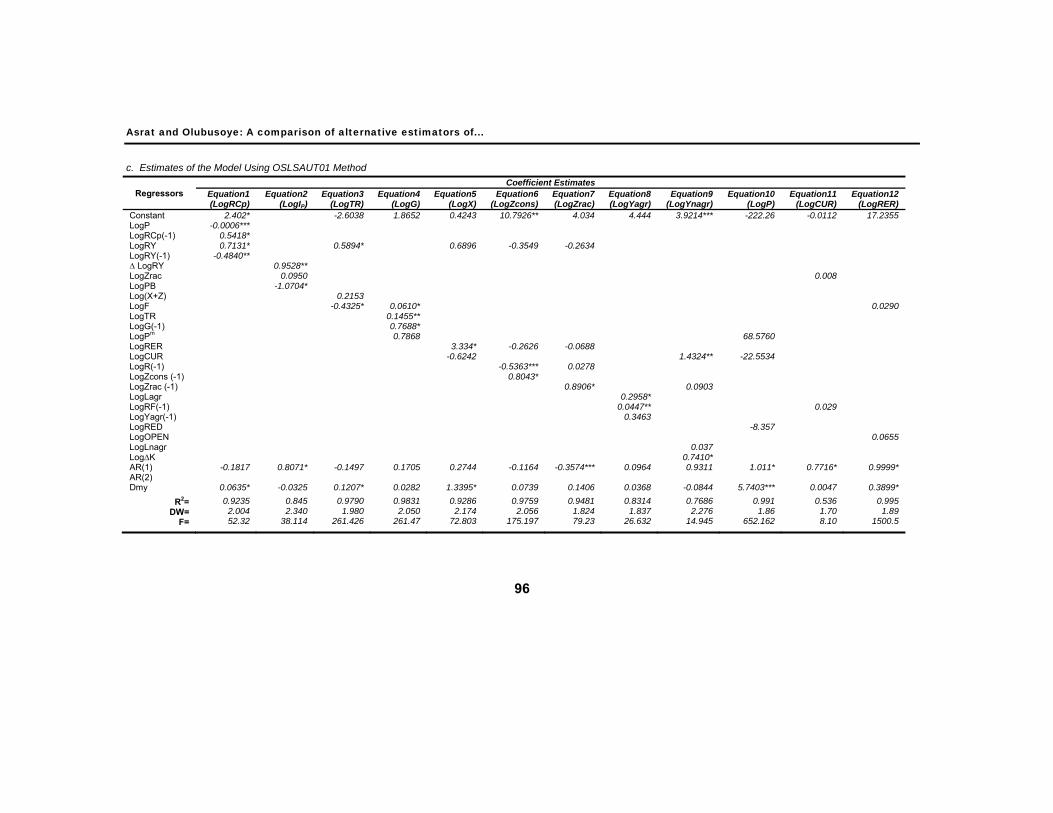
c. Estimates of the Model Using OSLSAUT01 Method


Equation1 (LogRCp)

Equation2 (LogIP)

Equation3 (LogTR)

Equation4 (LogG)

Equation5 (LogX)


Equation7 (LogZrac)

Equation8 (LogYagr)


Equation10 (LogP)

Equation11 (LogCUR)

Equation12 (LogRER)

Constant 2.402* -2.6038 1.8652 0.4243 10.7926** 4.034 4.444 3.9214*** -222.26 -0.0112 17.2355 LogP -0.0006*** LogRCp(-1) 0.5418* LogRY 0.7131* 0.5894* 0.6896 -0.3549 -0.2634 LogRY(-1) -0.4840** ∆ LogRY 0.9528** LogZrac 0.0950 0.008 LogPB -1.0704* Log(X+Z) 0.2153 LogF -0.4325* 0.0610* 0.0290 LogTR 0.1455** LogG(-1) 0.7688* LogPm 0.7868 68.5760 LogRER 3.334* -0.2626 -0.0688 LogCUR -0.6242 1.4324** -22.5534 LogR(-1) -0.5363*** 0.0278 LogZcons (-1) 0.8043* LogZrac (-1) 0.8906* 0.0903 LogLagr 0.2958* LogRF(-1) 0.0447** 0.029 LogYagr(-1) 0.3463 LogRED -8.357 LogOPEN 0.0655 LogLnagr 0.037 Log∆K 0.7410* AR(1) -0.1817 0.8071* -0.1497 0.1705 0.2744 -0.1164 -0.3574*** 0.0964 0.9311 1.011* 0.7716* 0.9999* AR(2) Dmy 0.0635* -0.0325 0.1207* 0.0282 1.3395* 0.0739 0.1406 0.0368 -0.0844 5.7403*** 0.0047 0.3899*

R2= DW=

F=

0.9235 2.004 52.32

0.845 2.340

38.114

0.9790 1.980

261.426

0.9831 2.050

261.47

0.9286 2.174

72.803

0.9759 2.056

175.197

0.9481 1.824 79.23

0.8314 1.837

26.632

0.7686 2.276

14.945

0.991 1.86

652.162

0.536 1.70 8.10

0.995 1.89

1500.5


97

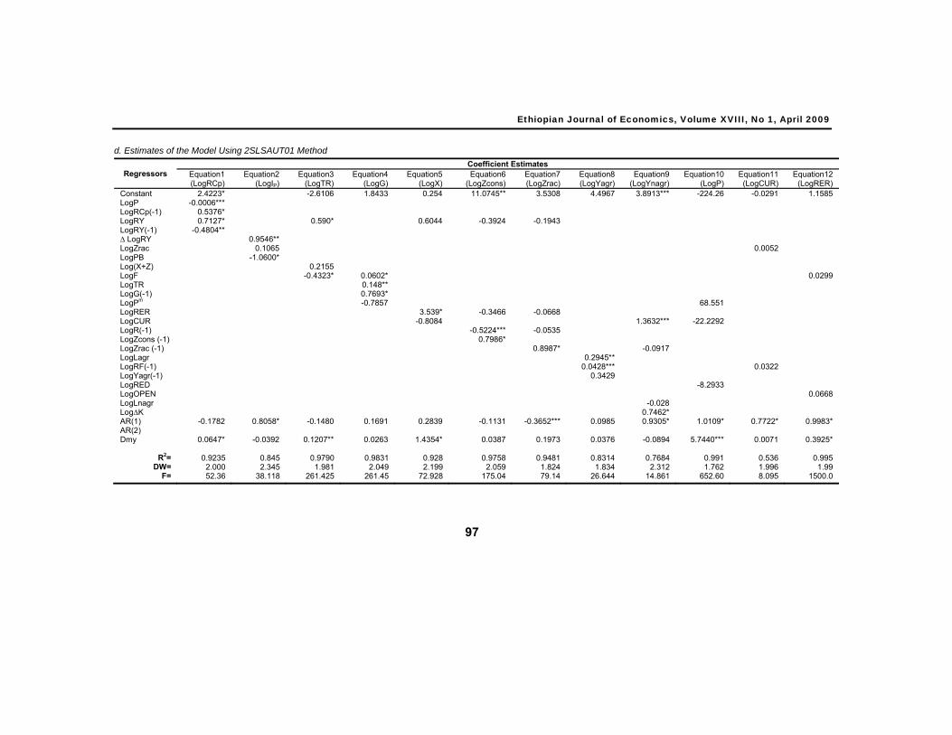
d. Estimates of the Model Using 2SLSAUT01 Method


Equation1 (LogRCp)

Equation2 (LogIP)

Equation3 (LogTR)

Equation4 (LogG)

Equation5 (LogX)


Equation7 (LogZrac)

Equation8 (LogYagr)


Equation10 (LogP)

Equation11 (LogCUR)

Equation12 (LogRER)

Constant 2.4223* -2.6106 1.8433 0.254 11.0745** 3.5308 4.4967 3.8913*** -224.26 -0.0291 1.1585 LogP -0.0006*** LogRCp(-1) 0.5376* LogRY 0.7127* 0.590* 0.6044 -0.3924 -0.1943 LogRY(-1) -0.4804** ∆ LogRY 0.9546** LogZrac 0.1065 0.0052 LogPB -1.0600* Log(X+Z) 0.2155 LogF -0.4323* 0.0602* 0.0299 LogTR 0.148** LogG(-1) 0.7693* LogPm -0.7857 68.551 LogRER 3.539* -0.3466 -0.0668 LogCUR -0.8084 1.3632*** -22.2292 LogR(-1) -0.5224*** -0.0535 LogZcons (-1) 0.7986* LogZrac (-1) 0.8987* -0.0917 LogLagr 0.2945** LogRF(-1) 0.0428*** 0.0322 LogYagr(-1) 0.3429 LogRED -8.2933 LogOPEN 0.0668 LogLnagr -0.028 Log∆K 0.7462* AR(1) -0.1782 0.8058* -0.1480 0.1691 0.2839 -0.1131 -0.3652*** 0.0985 0.9305* 1.0109* 0.7722* 0.9983* AR(2) Dmy 0.0647* -0.0392 0.1207** 0.0263 1.4354* 0.0387 0.1973 0.0376 -0.0894 5.7440*** 0.0071 0.3925*

R2=

DW= F=

0.9235 2.000 52.36

0.845 2.345

38.118

0.9790 1.981

261.425

0.9831 2.049

261.45

0.928 2.199

72.928

0.9758 2.059

175.04

0.9481 1.824 79.14

0.8314 1.834

26.644

0.7684

2.312 14.861

0.991 1.762

652.60

0.536 1.996 8.095

0.995 1.99

1500.0


98

e. Estimates of the Model Using OLSAUT02 Method


Equation1 (LogRCp)

Equation2 (LogIP)

Equation3 (LogTR)

Equation4 (LogG)

Equation5 (LogX)


Equation7 (LogZrac)

Equation8 (LogYagr)


Equation10 (LogP)

Equation11 (LogCUR)

Equation12 (LogRER)

Constant 2.2355* -2.3994 4.0276** -1.2105 11.867* -2.7219 2.3372 3.1382 -10696.29 -0.0197 6.2932 LogP -0.0004*** LogRCp(-1) 0.7303* LogRY 0.7171* 0.5866* 0.8505 -0.3569 0.3064 LogRY(-1) -0.6588* ∆ LogRY 0.5503 LogZrac 0.3799 0.0072 LogPB -0.7992* Log(X+Z) 0.1595 LogF -0.4740* 0.0664 0.0224 LogTR 0.3676** LogG(-1) 0.4536** LogPm -1.4550*** 60.418 LogRER 3.1498* -0.2050 -2.8388** LogCUR 0.4517 0.8435 -14.3822 LogR(-1) -0.6512** 0.8051*** LogZcons (-1) 0.8185* LogZrac (-1) -0.0642 0.0952 LogLagr 0.1528** LogRF(-1) 0.0752*** 0.0258 LogYagr(-1) 0.6373* LogRED -0.0913 LogOPEN 0.0450 LogLnagr 0.0905 Log∆K 0.8243* AR(1) -0.5745** 0.4411*** -0.24980 0.4306 0.1719 -0.2994 0.5587 -0.0887 0.6261* 1.2566* 0.9084* 1.3114* AR(2) -0.4946*** 0.3375 -0.1369 0.2233 0.1751 -0.3280 0.2684 -0.5485** 0.2981 -0.2564 -0.1958 -0.3119 Dmy 0.0522* -0.0115 0.1327** 0.0503 1.2637* 0.0737 -0.7558 0.0232 -0.1342 3.6809 0.0083 0.3897*

R2=

DW= F=

0.9323 1.940

47.193

0.853 1.984

30.186

0.9787 1.997

199.09

0.9834 2.148

211.965

0.932 1.97

59.606

0.9769 1.979

145.58

0.9581 2.085 78.41

0.8624 1.861 26.11

0.7859 2.033

13.111

0.992 1.814

522.09

0.549 1.846 6.331

0.9962

2.08 1421.36


99

f. Estimates of the Model Using 2SLSAUT02 Method


Equation1 (LogRCp)

Equation2 (LogIP)

Equation3 (LogTR)

Equation4 (LogG)

Equation5 (LogX)


Equation7 (LogZrac)

Equation8 (LogYagr)


Equation10 (LogP)

Equation11 (LogCUR)

Equation12 (LogRER)

Constant 2.2358* -2.4069 3.9912** 0.3149 11.9055* -2.4688 2.3682 3.1386 -12119.28 0.0321 1.2731 LogP -0.0004*** LogRCp(-1) 0.7302* LogRY 0.71698* 0.5865* 0.6971* -0.3624 0.2841 LogRY(-1) -0.6586* ∆ LogRY 0.5461* LogZrac 0.3873** 0.0034* LogPB -0.7924* Log(X+Z) 0.1615 LogF -0.4728* 0.0657 -0.0230 LogTR 0.3695** LogG(-1) 0.4563** LogPm -1.4554*** 60.6982* LogRER 3.4464*** -0.2169 -2.7057** LogCUR -0.6475* 0.8249 -13.2639 LogR(-1) -0.6488** 0.7782*** LogZcons (-1) 0.8178* LogZrac (-1) -0.0311 0.0969* LogLagr 0.1525* LogRF(-1) 0.0741** 0.0301*** LogYagr(-1) 0.6349*** LogRED -0.0379 LogOPEN 0.0459 LogLnagr 0.0921 Log∆K 0.8287* AR(1) -0.4943** 0.438*** -0.2471 0.4262 0.1727 -0.2996 0.5327 -0.0865 0.6205* 1.2449* 0.9127 1.3116* AR(2) -0.5742*** 0.340 -0.1327 0.22467 0.1426 -0.3273 0.2908 -0.5479 0.3035 -0.2447 -0.2016 -0.3140** Dmy 0.0522* -0.0134 0.1321** 0.0475 -1.4035 0.0687 -0.7021 0.0236 -0.1376 3.6746 0.0115 0.3913*

R2=

DW= F=

0.9323 1.740

47.195

0.853 1.985

30.193

0.9787

1.997 199.08

0.9834

2.15 211.933

0.932 1.982 59.40

0.9770

1.978 145.579

0.9581 2.074 78.29

0.8624 1.859 26.12

0.7859

2.035 13.112

0.9917 1.897

521.16

0.549

1.8476 6.326

0.9962

2.07 1421.26


100

a comparison of alternative estimators …ageconsearch.umn.edu/bitstream/249685/2/atsedeweyn and...

Documents