a comparative study for forecasting using neural networks vs genetically identified box&jenkins...

Neural Comput & Applic (1995)3:139-148 �9 1995 Springer-Verlag London Limited Neural

Computing & Applications

A Comparative Study for Forecasting using Neural Networks vs Genetically Identified Box&Jenkins Models

J o h n B l a k e 1, P e r e F r a n c i n o 2, J o s e p M. C a t o t 2 and Ignas i S016 2

1Faculty of Information and Engineering Systems, Leeds Metropolitan University, Leeds, UK; and 2Escola T~cnica Superior d'Enginyers Industrials, Universitat Polit~enica de Catalunya, Barcelona, Spain

This paper aims to discuss the results and conclusions of an extensive comparative study on the forecasting performance between two different techniques: a genetic expert system in which a genetic algorithm carries out the identification stage embraced in the three-phase Box&Jenkins univariate methodology; and a connectionist approach. A t the heart of the former, an expert system rules the identification- estimation-diagnostic checking cyclical process to end up with the predictions provided by the SARIMA model which best fits the data. We will present the connectionist approach as technically equivalent to the latter process and due to its, alas, lack of any conclusive existent algorithm able to identify both the optimal model and architecture for a given problem, the three most common models presently at use and 20 different architectures for each model will be examined. It seems natural that if a comparison is to be made in order to provide a straight answer as to whether or not a connectionist approach outperforms the univariate Box&Jenldns methodology, the benchmark should clearly be the set of time series analysed in the work 'Time Series Analysis. Forecasting and Control' by G. E. Box and G. M. Jenkins. Series BJA through to BJG give a total of 1200 plus measures to evaluate and compare the predictive power for different models, architectures, prediction horizons and pre-processing transform- ations.

Received for publication 18 July 1995 Correspondence and offprint requests to: Dr J.D. Blake, Faculty of Information and Engineering Systems, Leeds Metropolitan University, The Grange, Beckett Park, Leeds LS2 3QS, UK.

Keywords: Comparative study; Expert systems; Forecasting; Genetic algorithm; Neural networks; SARIMA models

1. Introduct ion

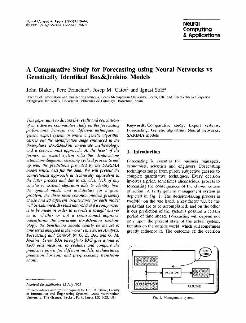
Forecasting is essential for business managers, economists, scientists and engineers. Forecasting techniques range from purely subjective guesses to complex quantitative techniques. Every decision involves a prior, sometimes unconscious, process to forecasting the consequences of the chosen course of action. A fairly general management system is depicted in Fig. 1. The decision-taking process is twofold: on the one hand, a key factor will be the goals that are to be accomplished; and on the other is our prediction of the system's position a certain period of time ahead. Forecasting will depend not only upon the present state of the actual system, but also on the outside world, which will sometimes greatly influence it. The outcome of the decision

f --,~

\

D E C I S I O N

t

Fig. 1. Management system.

140 J. Blake et al.

taken will depend upon how achievable was the goal and how accurate was the prediction.

Forecasting methods can be divided into two basic types (Fig. 2): qualitative methods and quantitative methods. Qualitative forecasting methods are those which use intuition and expertise to predict future events subjectively. Quantitative forecasting methods involve the analysis of historical data in an attempt to identify patterns that can be used to describe them. These descriptions or models can be then used to extrapolate the behaviour of the date into the future.

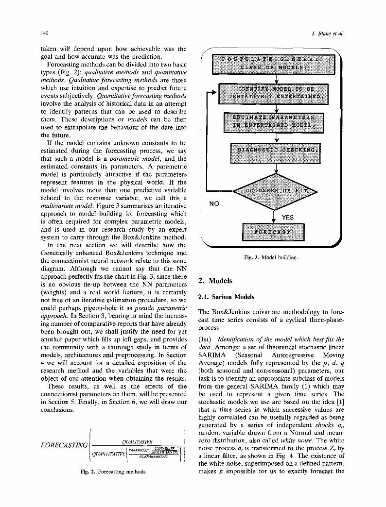
If the model contains unknown constants to be estimated during the forecasting process, we say that such a model is a parametric model, and the estimated constants its parameters. A parametric model is particularly attractive if the parameters represent features in the physical world. If the model involves more than one predictive variable related to the response variable, we call this a multivariate model. Figure 3 summarises an iterative approach to model building for forecasting which is often required for complex parametric models, and is used in our research study by an expert system to carry through the Box&Jenkins method.

In the next section we will describe how the Genetically enhanced Box&Jenkins technique and the connectionist neural network relate to this same diagram. Although we cannot say that the NN approach perfectly fits the chart in Fig. 3, since there is no obvious tie-up between the NN parameters (weights) and a real world feature, it is certainly not free of an iterative estimation procedure, so we could perhaps pigeon-hole it as pseudo parametric approach. In Section 3, bearing in mind the increasing number of comparative reports that have already been brought out, we shall justify the need for yet another paper which fills up left gaps, and provides the community with a thorough study in terms of models, architectures and preprocessing. In Section 4 we will account for a detailed exposition of the research method and the variables that were the object of our attention when obtaining the results.

These results, as well as the effects of the connectionist parameters on them, will be presented in Section 5. Finally, in Section 6, we will draw our conclusions.

ORECASTINGI ~ ~rvAmare , ~ 1 F QUALITATIVE

t . . . . . . . . . . . t J J Fig. 2. Forecasting methods.

m m l m m l m l m

NO

Fig. 3. Model building.

2. Models

2.1. Sarima Models

The Box&Jenkins univariate methodology to forecast time series consists of a cyclical three-phase- process:

(1st) Identification of the model which best fits the data. Amongst a set of theoretical stochastic linear SARIMA (Seasonal Autoregressive Moving Average) models fully represented by the p, d, q (both seasonal and non-seasonal) parameters, our task is to identify an appropriate subclass of models from the general SARIMA family (1) which may be used to represent a given time series. The stochastic models we use are based on the idea [1] that a time series in which successive values are highly correlated can be usefully regarded as being generated by a series of independent shocks a,, random variable drawn from a Normal and mean- zero distribution, also called white noise. The white noise process at is transformed to the process Zt by a linear filter, as shown in Fig. 4. The existence of the white noise, superimposed on a defined pattern, makes it impossible for us to exactly forecast the

Neural Networks vs. Genetically Identified Box&Jenkins Models 141

will seek models over an already fitted population, and in the part of the state space that does not comprise statistically non-significant parameters or non-invertible models.

Fig. 4. Linear filter.

next observation. The time series is regarded as a particular realisation of the underlying stochastic process:

dPp(B)c~p(B)VdVDZt = 0 o + ~)Q(B)Oq(n)at

B Backshift Operator B Z t = Z~-I (1)

The identification stage therefore consists of choosing the adequate degree of differencing and of the four polynomials ( p , d , q ) ( P , D , Q ) . It can be shown [2] that under certain conditions of a given process, (stationarity and invertibility) there is a unique relation between the shape of two of its functions plot, called the autocorrelation function and partial autocorrelation function, and the four polynomials' degree by which it is defined (1). We can, therefore, by taking control of the noise, filter the realisation and try to identify the process to which it belongs�9 Several authors describe other ways of tackling with the identification [3-5]. Our own purpose-built identification tool is a genetic algorithm (GA). In this approach, an initial population of randomly identified and estimated models, ranked according to a consistent information criterion, is used to apply the genetic reproduction, mutation and crossover operators. The algorithm gets closer to the optimum model at an over-exponential rate, as it is guaranteed by the Schema theory [6]. The process is continued until stability is reached�9 At this point, the system will have come upon a population of nearly alike 'fit' individuals, the best of which will be the solution model to the given time series.

(2nd) The entertained mode l is fitted to data and its parameters estimated�9 Whichever method we decide to use, once the model is chosen, basic statistics provide a wide variety of algorithms to find the optimal parameter estimates and to check their validiaty [7,8].

(3rd) Diagnostic checks are applied with the object of uncovering possible lack of fit and diagnosing the cause, with an open door to a new identification phase.

In the GA approach, if the information criterion is comprehensive enough, there is no need to go through phases 2 and 3 as separate stages during the model building process. The search algorithm

2.2. Connectionist Models

During the last ten years, many efforts have been undertaken to achieve a more effectve signal processing than within the linear models implicit in Box&Jenkins forecasting. Bilinear [9], threshold autoregressive [10] and the general state dependent models , to name just a few, are very promising examples of this work. The intricate non-linear model below describes a feed-forward neural network useful for forecasting purposes:

Zt = g(E~ wt~g(Ej w~ i . . (r . . g(wjt_lZ,_ 1

-~- W j t _ 2 Z t _ 2 Av . �9 �9 ' ~ - w j t _ i Z t _ i ) ) )

t = l , 2 , p . . . , t + p - 1 (2)

where data at time t and up to time t + p - 1 is a function of data down to time t - i , g is a function that accounts for the non-linearities, and Ws are the parameters to be estimated. Identification for this model would mean finding the appropriate values for the sigma index, j k . . . r, and for the number of past item Zt-1, . . . , Z t - i that Z t Z t _ 1

�9 . �9 Z~+p-1 are dependent on. Let us assume that there exists an efficient identification procedure and adequate non-linear function g. The next point we have to address is the estimation of the parameters Ws. Given the values for p and i during the identification, the assumption is that for every t the sequence Zt-1, . . . , Z t - i (a window of size i) is somehow related to the next sequence Zt, . . . , Z~+p_l, (a window of size p future in time), and that this relation is unknown and totally defined within the dataset.

If we shift both windows a certain step-width along the time series, this will add up a group of mapping datasets which are to be fitted during estimation, and therefore (2) should be a good approximation for each one of these datasets; the extension of (2) to each dataset will give

Zt ~ = g ( ~ wt~g('Zj w~j. . (r . . g ( w j t - l z , - i + wjt_2z,-2 + . . . + w,_iz,_i))) (3) t = 1 , 2 , p . . . . t

An error measure or global cost function will be

1 E ( w ) = (7",. - Z, )2

bti T = target or real value (4)

142 J. Blake et aL

which is clearly a continuous and differentiable function of every W as long as g is, so we can use a gradient descent rule to calculate the appropriate Ws:

6 E VWi j = -- V ~ Wij (5)

Bearing in mind Eq. (5) and moving our attention back to (1), it allows us to present graphically a way in which to carry through an automatic cost surface exploration by means of an oriented dynamic graph.

Zt -1 , . . �9 , Z t - i will be the input signal which, once processed towards the network output along the connections, weighted by the parameters W and squeezed through the functions g at each junction, will produce an output which we expect to be as close as possible to Zt, �9 �9 Zt+p-1 , this for every one of the mapping datasets. The error on each pattern can be used to change the weight values in a steepest descent direction of the weight-space surface, and repeat the process for the next pattern until the global error function reaches the desired minimum. The final weights structure will contain the valuable information which links throughout the whole training set each two successive patterns in time, and, hopefully, this bone will be maintained between the last of the patterns and the next, future, still unknown, data.

Equation (2) is by no means the only possible model available in the connectionist field. Any substantial change in the associated graph topology will have drastic effects on the updating rule, on the equation's appearance and, last but not least, on the pattern learning and recalling performance.

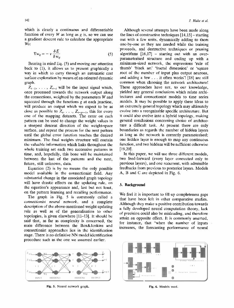
The graph in Fig. 5 is commonly called a connect ionis t neura l n e t w o r k , and a complete description of the above-mentioned weight updating rule as well as of the generalisation to other topologies, is given elsewhere [11-13]. It should be said that, as far as complexity is concerned, the main difference between the Box&Jenkins and connectionist approaches lies in the identification stage. There is no definitive NN model identification procedure such as the one we assumed earlier.

Although several attempts have been made along the lines of constructive techniques [14,15] - starting out with a few units, dynamically adding to them one-by-one as they are needed while the training proceeds, and destructive techniques or pruning algorithms [16,17] - starting out with an over- parameterised structure and ending up with a minimum-sized network, the expressions 'rule of thumb' 'black art' 'fractal dimension' or 'square root of the number of input plus output neurons, and adding a few . . . it often works'! [18] are still common when choosing the network architecture! These approaches have not, to our knowledge, yielded any general conclusions which relate architectures and connectionist models to time series models. It may be possible to apply these ideas to an extremely general topology which may ultimately evolve into a recognisable specific architecture. But it could also evolve into a hybrid topology, making general conclusions concerning choice of architecture a difficult task. At present there are only boundaries as regards the number of hidden layers as long as the network is correctly parameterised; one hidden layer is enough to map any continuous function, and two hiddens will be sufficient otherwise [19,20].

In this paper, we will use three different models, two feed-forward (every layer connected only to previous layers), and one recurrent, with admissible feedbacks from previous to posterior layers. Models A, B and C are depicted in Fig. 6.

3. Background

We feel it is important to fill up completeness gaps that have been left in other comparative studies. Although they make a positive contribution towards a fully developed neural computation theory, lack of precision could also be misleading, and therefore attain an opposite effect. It is commonly asserted, for instance, that "when the number of inputs increases, the forecasting performance of neural

Fig. 5. Neural network graph. Fig. 6. Models used.


network improves. More inputs will provide more information, and hence will provide more accurate forecasts" [21]. This we have found to be inexact in our comprehensive study using the NN models indicated. Comparative trials on connectionist models should account for a sufficient variety of topologies, inputs, hidden units, hidden layers and steps ahead, so as to enable the authors to take a stand on the conclusions.

Since more than two hidden layers provide no better chance of learning the training patterns, we have used two hidden layers for both feed-forward architectures. For each connectionist model three steps ahead will be tested (2, 5 and 10) for each trial; the number of inputs will be 1, 2, 4, 6, 8; and the number of hiddens for each input will be 2, 6, 10 and 14 (the same for both hidden layers). When the model is either non stationary or seasonal, the network will be tried with both transformed and raw data.

We approach the problem of overfitting by using internal validation [22], so we can relax the study of the number of hidden units relative to different hidden layers by choosing the same number of units for both layers.

3.1. Data

Varfis and Versino [23] report their work on an original network topology, which encodes in its input units, besides the normal past values of the time series, the seasonal and the trend pattern. They base their conclusive similar performance on two time series. De Groot and Wiirtz [24] make an interesting comparison between an autoregressive model, a bilinear, a threshold autoregressive and a connectionist model, and also base their conclusions on two well-known time series, the sunspots activity data and a deterministic chaotic series with a white noise component. Baestens et al. [25] report an outperforming neural network compared to an ARIMA model using a single 45 scaled monthly data time series. Tang et al. [21] report a better neural network performance for long-term forecasting and short memory time series based on two SARIMA models; airline data and car sales.

Our benchmark will be the set of time series analysed by Box&Jenkins in the book with which the SARIMA modelling theory was born. Real series BJA through to BJG include both the sunspots and the airline passengers data. There are cases of seasonality and non-seasonality, stationarity and non-stationarity in mean, and stationarity and nonstationarity in variance.

3.2. Time Series Models

The majority of people who are working on a daily basis with SARIMA models to forecast real-time series will rarely find models with degrees of the regular autoregressive polynomial higher than 4, seasonal autoregressive higher than 3, regular moving average higher than 3 and seasonal moving average higher than 2, as well as differencing higher than 2 if it is regular or 1 if seasonal. Consequently, most of comparative benchmarks for this technique need not go far beyond these limits. The sunspots activity data is one of the author's favourite series with which to test NN forecasting ability, and although it is a challenging time series for an everyday forecaster, it is not one you are often likely to meet - TAR(2,4,12) [26].

4. The Method

A summary of the way in which we have proceeded for each time series is presented in Fig. 7.

Each time series was divided in three sets: Training, Test and Forecasting. The forecasting set was that part of the data strictly kept apart and only used to test the performance of the estimated network. The test set or internal validation set was an equidistant extraction of the available data after the forecasting set had been chosen. It was correctly pre-processed in the form of input-output patterns to feed the network according to its architecture. Its purpose was not to estimate the parameters, but to determine the stopping point of the training process. The remaining part of the series formed the training set. This was that part of the data used to strictly estimate the parameters. Ultimately, we were interested in good performance for patterns which the network had never 'seen' before or used to estimate the parameters; it was its ability to

: ' for each da ta set c h o o s e f o r e c a s t i n g se t

> for each NN m o d e l I for each a r c h i t e c t u r e

c h o o s e t r a i n i n g and t e s t se t t r a i n e v a l u a t e on f o r e c a s t i n g set

>

f i n d S A R I M A m o d e l > f o r e c a s t and e v a l u a t e

Fig. 7. Time series.

144 J. Blake et al.

generalise what we were seeking, not to memorise. Hence, presenting the test set at a certain number of iterations in the training process stopped when the test error worsened for a prolonged period of time, even if the training error was falling, which was usually the case. The test set was not used to update the weights. As an evaluation parameter, the mean squared error (MSE) and the average relative variance (ARV), which is the MSE normal- ised by the variance, were used for the forecasting set.

The size of the test and training set depend upon the architecture, since the total number of patterns varies with the number of inputs. The last ten data items were kept to forecast in time series B, C, D and G, seven five and eight for series A, E and F. The criterion for choosing the forecasting set was to include a sudden change of tendency, as much as the stationarity assumption allows it to happen. The remaining data was pre-processed in patterns according to the architecture and a 12%, equidistant set of the total amount was designated as the test set.

The last percentage followed advice [22] of a number between 10% and 15%. The learning was set to 0.1 and the momentum term to zero. Pattern selection during training was set to random, except for the recurrent architecture.

5. The Results

The results are a collection of 30 tables, one of which is shown in the appendix. Each of the 30 tables contains information on the performance of each of the 10 time series ( B J A . . . BJG plus BJBD, BJCD and BJGLSD transformed for stationarity and non-seasonality of BJB, BJC and BJG, respectively), with one of the three connectionist models (back- propagation, jump connection and recurrent). Our

main concern on starting this research work was to answer the following questions: Is there any significant difference between the performance of different connectionist models? Is there any favourite or neglected architecture? Is a connectionist model able to predict an out-of-sample set of non- stationary or seasonal patterns, or do we need to reprocess the data? And last but not least: Can we ensure that a NN model is, in general, able to outperform a SARIMA model or, as suggested in [27], does this happen only with short memory time series and long-term forecasts?

5.1. Architectures

Figure 8 shows, for each different model and forecasting horizon, across all the time series, which architectures produce the best performance, i.e. for the recurrent model and long-term forecasting (RCL), eight inputs and ten hidden units (8,10) gave the best performance for one time series. In the case of a draw, both architectures have been depicted. Thus, for eah model, the number of hits for a particular architecture is the number of time series that were best modelled by that architecture.

As we expected, there is no favourite architecture and, more important, there is no obvious improve- ment with an increasing number of inputs or hidden units.

There is, however, a clear tendency for the four- inputs architecture to perform poorly, regardless of the model and the time series.

5.2. Models

Figure 9 shows, for each time series (vertically), which of the three architectures (recurrent, jump connection or back-propagation) produced the best five performances in the short, medium- and long-

b 14~

10 8 6 4 2 0

~._" ,__" ,-- ~ c~d c,a" ~ ~ ~-" ,n-" ~ , - t.o" c d *-- , ' - co" c~" ,--. ~

Architecture

Fig. 8. (a) Architecture vs. long-, medium- or short-term forecasting model (BPS: back-propagation short-term forecasting; JCM: jump connection medium-term forecasting; RCL: recurrent long-term forecasting; BPL: back-propagation long-term forecasting; RCS: recurrent short-term forecasting); (b) number of 'hits' per architecture.


Fig. 9. Best performance figures.

the medium-term the best five performances were produced by the recurrent architecture. The fifth coloured cell in JCM means that there was a draw, and the fifth of the best five performances for the medium-term was also produced by the jump connection architecture.

It can clearly be seen how each connectionist model appears to be adequate for a certain type of time series. Although a priori only two categories could be found (stationary and non-stationary), it is the actual table that singles out a third group of series: the time series in which stationarity has been attained by pre-processing the data. The back- propagation model seems to work fine for this type of data, yet if it is not pre-processed, the jump connection gives better results than the other two models. The recurrent model is the best at forecasting originally stationary data.

Fig. 10. Best ARV from among the models and architectures for pre-processed and non pre-processed data.

term. The best of these five for each time period has been coloured the darkest, and the worst is lightest. Thus, all five cells for series bja and model RCM are coloured, because for time series bja and

5.3. Is Pre-processing Always Necessary?

It turns out from Fig. 10 that, for a number of series, pre-processing is necessary, but is less important than choosing the correct architecture and connectionist model. As will be seen in the next section, all the best ARV, outperform the

146 J. B lake et al.

Table 1. Set series and their corresponding model, periodicity and size.

Source Size Period SARIMA

BJA Chemical process concentration 197 2 hours BJB IBM common stock closing prices 369 daily BJC Chemical process temperature 226 1 minute BJD Chemical process viscosity 310 1 hour BJE Sunspot activity 100 1 year BJF Yields from batch chemical process 70 - - BJG International airline passengers 144 1 month

(101) or (011)

(011) (110) or (022) (100) or (011) (200) or (300)

(200) (011) *(011)12

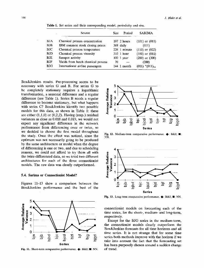
Box&Jenkins results. Pre-processing seems to be necessary with series G and B. For series G to be completely stationary requires a logarithmic transformation, a seasonal difference and a regular difference (see Table 1). Series B needs a regular difference to become stationary, but what happens with series C? Box&Jenkins identify two possible models for this data, as shown in Table 1: these are either (1,1,0) or (0,2,2). Having (resp.) residual variances as close as 0.018 and 0.019, we would not expect any significant difference in the network performance from differencing once or twice, so we decided to choose the first model throughout the study. Once the effect was noticed, since the optimum was not necessarily going to be produced by the same architecture or model when the degree of differencing is one or two, and due to scheduling reasons, we could not afford to try them all with the twice-differenced data, so we tried two different architectures for each of the three connectionist models. The raw data was clearly outperformed.

5.4. Sarima or Connectionist Model?

Figures 11-13 show a comparison between the Box&Jenkins performance and the best of the

5

,-~ 4

� 9

0 if3 ..Q "o O -o 13 ~3~ ~3~ "O

(-) ..Q

Series

Fig. 11. Short-term comparative performance. , : B&J; lU: NN.

e u 3 n- r ~,_~

0

._Q .-Q _Q

Series

Fig. 12. Medium-term comparative performance. ~ : B&J; n : NN.

4 :1,

"~ 3 _~�9 fa

=|2 I~1 'm

= 1 :1.

',E

0 ~l ..Q

_Q ..Q "0 t.) "(3 "0 ~ ~yl -~

~- .~ ~ -Q o - . _ _ ,

Ser ies

Fig. 13. Long-term comparative performance. 4~: B&J; n: NN.

connectionist models on forecasting each of the time series, for the short-, medium- and long-term, respectively.

Except for the BJG series in the medium-term, the connectionist models clearly outperform the Box&Jenkins forecasts for all time horizons and all time series. It is not strange that for some time series both methods improve with the horizon if we take into account the fact that the forecasting set has been purposely chosen around a sudden change of trend.


6. Conclusions

Neural networks appear to be a future alternative to Box&Jenkins forecasting in all circumstances, and if they are not already so it is only due to the lack of a defini t ive identification procedure. This, together with our success in using a G A as a searching algorithm for the S A R I M A model, calls to mind a genetic approach for the identification of the opt imum neural network. Several at tempts are being undertaken at present in this area, and it is our understanding that this topic is worth investigating further. Our work has proven that a correctly identified and trained neural network produces bet ter forecasts than a S A R I M A model. Key factors in obtaining the best results are the internal validation during the training process, the data pre- processing when it is a non-stationary series, and the choice of adequate connectionist model, depending on whether the data is stationary or not. It has also been shown that the connectionist forecasting ability does not necessarily improve with the number of inputs nor hiddens, and that pre- processing, although not essential to outperform B&J, further enhances the neural network ability.

References

1. Yule GU. On a method of investigating periodicities in disturbed series. Phil Trans 1927; A226:267

2. Box GEP, Jenkins GM. Time Series Analysis-Forecasting and Control, Holden-Day, San Francisco, 1976

3. Vails M. Identificaci6 Autom/~tica de S~ries Tem- porals, PhD Thesis, UPC Barcelona, 1983

4. Akaike H. A new look at the statistical model identification. IEEE Trans Auto Control 1974; AC- 19:716-723

5. Burg JP. Maximum Entropy Espectral Analysis, PhD Thesis, Stanford University, 1975

6. Goldberg DE. Genetic Algorithms in Search: Optim- ization and Machine Learning. Addison Wesley, CA, 1989

7. Tsay RS, Tiao GC. Consistent estimates of autore-

gressive parameters and extended sample autocorrelation function for stationarity and nonstationarity ARMA models. J Am Statist Assoc 1984; 79:84-96

8. Pankratz A. Forecasting with Univariate Box-Jenkins Models. John Wiley & Sons, New York, 1983

9. Granger C, Anderson T. An Introduction to Bilinear Time Series Models. Vandenhoeck and Ruprecht, Gottingen, 1978

10. Tong H. Threshold Models in Non-linear Time Series Analysis: Lecture Notes in Statistics. Springer-Verlag, Berlin, 1983

11. Hertz J, Krogh A, Palmer R. Introduction to the theory of neural computation. Addison-Wesley, CA, 1991

12. Freeman J, Skapura D. Neural Networks Algorithms, Application. Addison-Wesley, CA, 1991

13. McClelland J, Rumelhart D. Parallel distributed processing. MIT Press, MA 1988

14. Refenes A. Constructive learning and its application to currency exchange rate forecasting, 1990

15. Gallant S. Three constructive algorithms for neural learning. 8th Ann Conf Cog Sci Soc, 1986

16. Pelillo M, Fanelli M. A method of pruning layered Feddforward NNs. Proc IWANN '93, 1993

17. Karnin E. A simple procedure for pruning BP trained NNs. IEEE Trans Neuro! Networks 1990; VI: 325-333

18. Eberhart R, Dobbins R. Neural Network PC tools a practical guide. Academic Press, CA, 1990

19. Cybenko G. Continuous valued Nns with 2 hidden layers are sufficient. Technical report, Tufts Univer- sity, MA, 1988

20. Cybenko G. Approximation by superpositions of a sigmoidal function. Math Control, Signals Syst 1989; 303-313

21. Tang Z, Almeida C, Fishwick D. Time series forecasting using NNs vs. B&J methodology. Simula- tions 1991

22. Weigend A, Huberman B, et al. Predicting the future; a connectionist approach. Intl J Neural Syst 1990; VI: 193-209

23. Varfis A, Versino C. NNs for economic time series forecasting. Proc ICANN'90, 1990

24. Groot C, Wfirtz D. Analysis of univariate time series with connectionist nets. Proc. ICANN'90, 1990

25. Baestens D, Bergh W, et al. Estimating tax inflows at a public institution. Proc. NN Capital Markets, 1993

26. Tong H, Lira K. Threshold Autoregression, limit cycles and cyclical data. RSS 1980; B42:245

27. Sharda R, Patil R. Connectionist approach to time series prediction: an empirical test. J Intell Manuf 1992; 3:317-323

148

A p p e n d i x

Table A1. Example results table.

SERIE: BJC SIZE: 226 PERIOD: 1 MINUTE Box & Jenki~

MODEL: JUMP CONNECTION (NETWORK)

HIDDENS

HORIZON: 2

INPUTS: 1

AVERAGE RELATIVE MEAN SQUARED ERROR VARIANCE

HIDDENS

2 6 10 14 2 6 10 14

0.67 0.43 1.08 1.01 0.03 0.015 0.04 0.04

0.85 1.48 1.48 1.9 0.03 0.06 0.06 0.08

2.33 2.20 3.21 2.44 i 0.09 0.09 0.13 0.10

0.86 1.23 1.79 0.86 0.03 0.05 0,07 0.03

81 4.42 3.63 3.63 4.91 0.18 0.15 0.15 0.20

CII0) OR (022)

ARV I MSE

0.45 I 0.02

,oP~zoN:5 I 2 6 10 14 2 6 10 14 088 1 0 . 4 4 i

I INPUTS: 1 1 0.86 1.28 1.22 0.5 0.40 0.64 0.61

2 1.46 2.07 2.07 3 0.73 1.04 1.04 1.6

41 2.71 2.73 3.57 2.90 1.36 1.37 1.79 1.46

61 1.40 1.79 2.17 1.33 0.70 0.90 1.09 0.67 I

8 3.96 3.80 3.73 4.65 1.99 1.91 1.87 2.34

HORIZON:10 2 6 10 14 2 6 10 14 0.99 [ 1.37

INPUTS: 1 1.18 0.95 1.49 1.40 1.63 1.25 2.05 1.93

2 2,12 2.94 2.99 3.5 2.92 4.06 4.12 4.9

4 4.19 4.66 5.83 4.85 5.78 6.43 8.04 6.69

6 2.0I 2.71 3.39 1.71 2.77 3.74 4.68 2.36

8 5.87 6.15 6.52 7.32 8.09 8.48 9.0 10.10

J. Blake et al,

This appendix contains one example of the complete set of 30 tables and its correspondent figure for medium term forecasting. In this case, the Back Propagation model for series C shows a minimum for one input and six hidden units, and a clear tendency to worsen in performance as the number of units increases.

Fig. A1. Example results chart.

a comparative study for forecasting using neural networks vs genetically identified box&jenkins...

Documents