0

August 2010

Prepared for the Forum of Labour Market Ministers (FLMM) Labour Market Information Working Group (LMIWG)

Souleima El Achkar CSLS Research Report 2010-07

August 2010

CENTRE FOR THE

STUDY OF LIVING

STANDARDS

A COMPANION GUIDE TO ANALYZING AND PROJECTING

OCCUPATIONAL TRENDS

111 Sparks Street, Suite 500 Ottawa, Ontario K1P 5B5

613-233-8891, Fax 613-233-8250 csls@csls.ca

i

A Companion Guide to Analyzing and Projecting Occupational Trends

Abstract

This report is intended to complement Future Labour Supply and Demand 101: A Guide

to Analysing and Predicting Occupational Trends, a technical document commissioned

by the Forum of Labour Market Ministers (FLMM) Labour Market Information Working

Group (LMIWG) with the aim of achieving greater consistency and coordination in

labour supply and demand modeling in Canada. In conjunction with the technical

document, this companion guide will assist stakeholders in making informed decisions

regarding the occupational modeling needs of their organizations.

ii

A Companion Guide to Analyzing and Projecting Occupational Trends

Table of Contents Abstract ................................................................................................................................ i

Executive Summary ........................................................................................................... iii

I. Introduction ......................................................................................................................1

II. Occupational Forecasting and the Labour Market ..........................................................3 A. A Changing Economy and Labour Market .................................................................3 B. Labour Market Concepts: Demand, Supply, Equilibrium and Imbalances .................3

C. The Role of Occupational Modeling and Forecasting .................................................5

III. Developing a Basic Occupational Forecasting Model ...................................................6 A. Initial Considerations in Developing a Labour Supply and Demand Model ..............6

B. Assumptions, Variables and Coefficients ....................................................................6 C. Forecasting Techniques ...............................................................................................7 D. Basic Structure of a Labour Supply and Demand Model ............................................7

E. Detailed Steps Involved in the Development of a Baseline Model .............................9 Stage 1: Demand Side ..................................................................................................9

Stage 2: Supply Side ...................................................................................................10 Stage 3: Balancing supply and demand – Identifying future imbalances ..................12

F. Simplifying or Expanding the Model .........................................................................12

IV. Limitations of Occupational Modeling and Forecasting .............................................14

V. A Road Map to Undertaking Labour Supply and Demand Modeling and

Forecasting .........................................................................................................................16 A Road Map for Government .........................................................................................16 A Road Map for Educational Institutions ......................................................................17

A Road Map for Industry ...............................................................................................18

Bibliography ......................................................................................................................19

Annex 1 – Glossary of Basic Terminology........................................................................21

Annex 2 – A List of Additional Resources ........................................................................23

Annex 3 – Examples of Occupational Forecasting Models ...............................................24 A. Canadian COPS model ..............................................................................................24 B. BC Education Model .................................................................................................26

C. Alberta Occupational Demand and Supply Outlook Models ....................................26 D. Construction Sector Council Model ..........................................................................28 E. Dutch ROA Model .....................................................................................................29

iii

A Companion Guide to Analyzing and Projecting Occupational Trends

Executive Summary

The Labour Market Information Working Group (LMIWG) of the Forum of

Labour Market Ministers (FLMM) commissioned the development of a guide to

projecting future occupational supply and demand trends and imbalances. This was done

with the aim of achieving greater consistency and coordination in labour supply and

demand modeling in Canada. The guide, a technical document entitled Future Labour

Supply and Demand 101: A Guide to Analysing and Predicting Occupational Trends,

was prepared by the Centre for Spatial Economics.

This companion guide, prepared by the Centre for the Study of Living Standards,

is intended to complement the technical document and assist stakeholders in making

informed decisions regarding the occupational modeling needs of their organizations.

Many factors influence labour market trends. These factors may be associated

with short-term business cycle fluctuations, or with longer-term structural developments

in the economy including technological progress, demographic change, and globalization.

In the face of such uncertainty, labour market stakeholders, such as workers, employers,

and governments, must make decisions about education and training, hiring, and

investment – decisions that will affect the future supply of and demand for jobs and

workers across a variety of sectors and occupations. Occupational forecasting modes can

be useful tools to assist stakeholders in their decision-making and to help prevent costly

labour supply and demand imbalances in the future.

Any economic modeling exercise requires decisions about what variables to

include, how to model the relationships between the variables, and what underlying

assumptions to make. There is no single best approach. The choice of model should

depend on the ultimate need that the forecasting model will fulfill, the resources available

for the development of the model, and the availability and quality of data. This report

provides guidelines for the development of occupational forecasting models to suit the

needs of various stakeholders, including firms, government departments, labour unions,

and educational institutions.

There are several limitations to occupational modeling and forecasting. The

accuracy of a model‟s forecasts depends on the soundness of the macroeconomic scenario

on which the model is based. Measurement error in the variables and inappropriate

assumptions about them may result in inaccurate forecasts. To some extent, there is a

trade-off between accuracy and cost; more accurate forecasts will require more complex

and costly models that account for a wider variety of relevant factors. Different

stakeholders may make different choices with respect to this trade-off, depending on their

particular forecasting needs.

1

A Companion Guide to Analyzing and Projecting Occupational Trends

I. Introduction1

Purpose of the Report

In the absence of a pan-Canadian labour supply projection model that would

enable analysis at the provincial and sub-provincial levels, the Labour Market

Information Working Group (LMIWG) of the Forum of Labour Market Ministers

(FLMM) identified the need for a practical approach to achieve greater consistency and

coordination in labour supply and demand modeling in Canada. To achieve this objective,

the LMIWG commissioned the development of a guide to projecting future occupational

supply and demand trends and imbalances, which would serve as a useful tool for

stakeholders. The guide, a technical document entitled Future Labour Supply and

Demand 101: A Guide to Analysing and Predicting Occupational Trends, was prepared

by the Centre for Spatial Economics.

This companion guide is intended to complement the technical document, and

assist stakeholders in making informed decisions regarding the occupational modeling

needs of their organizations.

Structure of the Report

The guide will be divided into four major sections after the introduction. Section

II will describe the rapidly changing economy and labour market, the factors determining

labour demand and supply (e.g. business cycle, demographic structure, etc.), the

relationships between these factors, and the linkages between these factors and projected

labour market outcomes. The section will provide an overview of relevant concepts (e.g.

skill gaps, labour market imbalances, workforce shortages, skills demands, skills

mismatches) and highlight the role of modeling and forecasting in identifying potential

imbalances.

The third section will review the key considerations when developing an

occupational projection model, and provide the basic structure of the model. It will

outline the model and describe the steps involved in its development, the role of

occupational and industry categories, the required components and inputs, and the

forecasting techniques. This section will underline the key elements of a baseline model

in non-technical terms, and will briefly explain how it can be expanded or modified to

resemble a number of existing occupational forecast models.

1 This report was written in March 2009 while the author was an economist at the Centre for the Study of Living

Standards (CSLS). It was written under the supervision of CSLS Executive Director Andrew Sharpe. The author would

like to thank members of the Forum of Labour Market Ministers Labour Market Information Working Group for

comments, and Jean-François Arsenault and Alexander Murray of the CSLS for editorial assistance.

2

The fourth section will briefly discuss the limitations of occupational modeling,

including forecasting accuracy issues and data and resource availability issues.

Section V will provide stakeholders who wish to undertake labour supply and

demand modeling and forecasting with a road map, that is, a tool to identify and develop

a model that is suitable for them. Depending on their needs, resources and capacity

constraints, organizations may benefit from forecast models that differ in their

complexity and focus (e.g. occupations, education or skills).

Finally, a glossary of basic terminology and a list of additional resources related to

modeling and forecasting, including publications, websites and agencies, will be provided

in an appendix. Additional resources will include a detailed list of available labour

market data sources for Canada.

3

II. Occupational Forecasting and the Labour Market

A. A Changing Economy and Labour Market

There are a number of factors affecting the supply and demand of labour. These

factors may be cyclical, related to short-term fluctuations in aggregate demand, or

structural, reflecting long-term trends or developments in the economy or society,

independent of short-term fluctuations. Structural factors include technological advances,

the globalization of competition, and changes in the demographic composition of the

population.

Technological change has had a major impact on the occupational structure of

many countries by shifting their industrial structure (e.g. from primary and manufacturing

industries to services, in Canada) and by increasing the demand for highly skilled work

relative to that for less skilled work – a phenomenon referred to as „skill-biased‟

technological change.

Globalization also affects occupational structure, by shifting the industrial

structure of countries.2 In addition, a number of researchers have suggested that

globalization increases the need for high-skilled labour in advanced economies, and

reduces the demand for low-skilled labour. There is also evidence that globalization has

contributed to a reduction in wage differentials across countries for labour of similar skill

level, but has (along with technological change) led to an increase in wage inequality

between lower and higher skill levels within high-wage countries.

Demographic factors in the context of Canada and most industrialized economies

generally refer to the increasing average age of the workforce, with fewer entrants and a

large number of retirees as the baby boomers cohort reaches retirement age. Other factors

that are having an impact on skill requirements and occupational demand include

competition and changing patterns of consumer demand, changing work practices and

regulatory changes and increasing concern about environmental issues.

Given the rapidly changing economy and labour market conditions, occupational

projection models and forecasts need to be constantly updated to reflect new

developments.

B. Labour Market Concepts: Demand, Supply, Equilibrium and Imbalances

Occupational demand refers to the number of workers required by employers for

an occupation, given a certain wage level. By definition, therefore, it includes the number

of workers employed as well as the number of vacant positions that employers would like

to fill for this occupation. Occupational supply refers to the number of workers employed

2 Economic theory predicts that globalization will shift the industrial structure of countries towards their export sectors,

which are the sectors that use their relatively abundant factors of production more intensively.

4

or seeking employment in an occupation, given the existing labour market conditions

(primarily, at a certain wage level). Occupational supply may be referred to as the

occupation‟s labour force.

When the occupational demand and supply are equal, the labour market for the

occupation is said to be in equilibrium. A divergence between labour demand and supply

is a labour market imbalance. There are two types of labour market imbalances: excess

supply (unemployment) and excess demand (labour shortages).

Labour market imbalances attributable to the business cycle are by definition

temporary. However, imbalances can also arise from structural factors such as

technological change (e.g. new technologies resulting in a shortage of new skills that

workers have not had opportunity to acquire, or reducing the need for workers to perform

specific tasks) or demographic factors (e.g. a high number of retirements). Inefficient

education investment decisions can also result in imbalances (e.g. shortage of doctors or

civil engineers).

A labour market adjustment occurs when labour demand or labour supply shift

so as to eliminate or reduce an imbalance. For instance, when confronted with a labour

shortage, adjustments by firms include raising wages, providing additional training to the

existing workforce, substituting the scarce labour for capital or for some other type of

labour, and in some cases, attempting to move production to a different location. Labour

market adjustments by workers include acquiring new skills that are in demand, or

moving to a geographic area where there are vacancies due to labour shortages.

Labour market adjustments generally do not take place instantaneously,

however. A lack of information, the time required for training or re-training (particularly

for high skilled occupations), and various institutional barriers to labour market

adjustment mean that in a given place at a given time there will be gaps between the

quantities supplied and demanded for particular skills. For instance, employers may be

unable to raise wages due to inflexible compensation structures or because doing so

reduces their international competitiveness. Obstacles to regional labour mobility can

also contribute to shortages. Moreover, firms and individuals simply may not recognise

the signals of changes in the labour market in order to react to them (e.g. raise wages or

invest in training); slow response time may delay market adjustment.

It is important to note that even if all imbalances were temporary (due to labour

market adjustment), a shift in labour demand and/or labour supply resulting in a different

equilibrium may be preferable for various reasons.3

3 Although many would consider labour market imbalances temporary, the literature on multiple equilibria

emphasises that economies may get stuck at various states depending on their histories. Some of these

perhaps rather stable equilibria can be more desirable for a society than others.

5

C. The Role of Occupational Modeling and Forecasting

By providing information for employers, employees and policymakers,

occupational forecasting facilitates a labour market balance and reduces adjustment costs;

increases productivity and efficiency; and reduces social and economic problem arising

from labour market imbalances (e.g. a shortage of doctors, social problems associated

with high unemployment). It also helps ensure that workers are employed in occupations

that correspond to their skill level, resulting in significant productivity and efficiency

gains.

Occupational forecasting also improves personal and public investment decisions,

and in particular decisions pertaining to education. Individuals often lack the information

and the incentives necessary to invest in acquiring the knowledge and skills that will be

required in the future. This leaves government with a dual role: identifying the skills that

will be in high demand in the future and the areas where shortages may occur (through

occupational forecasting) and subsidizing education.

In addition to providing information, occupational models can illustrate potential

implications of a change in assumptions, including a change in government policy, on

future labour market developments (Centre for Spatial Economics, 2005).

Today, the use of occupational modeling and forecasting is widespread. Most

models used are national in scope, although sub-national components are also available,

such as provincial models for Quebec and Alberta.

6

III. Developing a Basic Occupational Forecasting Model

A. Initial Considerations in Developing a Labour Supply and Demand Model

There is no one ideal occupational forecasting approach or model for all

stakeholders. The choice of model and approach for each organization or stakeholder

depends on a number of factors:

The ultimate need that the forecasting model fulfills:

who are the end users of the forecast and/or whose perspective does the

model need to convey?

what is the desired output format?

The amount of resources committed to the task: a more complex and comprehensive

model requires more resources

Data availability, quality and coverage, which depend on:

the source of the data (Canadian labour market data sources are listed in

Annex 2)

the level of detail or disaggregation required (whether the forecast is for an

occupation vs. occupational group, industry vs. sector)

These issues, as well as the steps described below are combined in a flow chart in

Section V, providing the user with a road map to occupational forecasting.

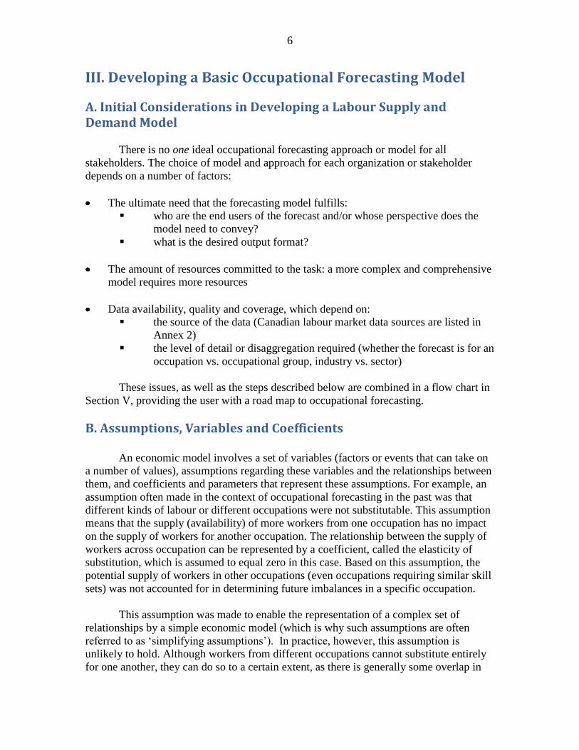
B. Assumptions, Variables and Coefficients

An economic model involves a set of variables (factors or events that can take on

a number of values), assumptions regarding these variables and the relationships between

them, and coefficients and parameters that represent these assumptions. For example, an

assumption often made in the context of occupational forecasting in the past was that

different kinds of labour or different occupations were not substitutable. This assumption

means that the supply (availability) of more workers from one occupation has no impact

on the supply of workers for another occupation. The relationship between the supply of

workers across occupation can be represented by a coefficient, called the elasticity of

substitution, which is assumed to equal zero in this case. Based on this assumption, the

potential supply of workers in other occupations (even occupations requiring similar skill

sets) was not accounted for in determining future imbalances in a specific occupation.

This assumption was made to enable the representation of a complex set of

relationships by a simple economic model (which is why such assumptions are often

referred to as „simplifying assumptions‟). In practice, however, this assumption is

unlikely to hold. Although workers from different occupations cannot substitute entirely

for one another, they can do so to a certain extent, as there is generally some overlap in

7

skills across occupations (particularly within the same occupational group). Thus, a more

realistic assumption is that the elasticity of substitution varies between zero and one, and

takes on higher values for occupations that are either low-skilled or require similar skill

sets. In fact, the assumption of zero substitution has been highlighted as an important

weakness of occupational forecasting in the past. New models generally account for

inter-occupational mobility in some way, although there is not yet a standard way of

doing so.

Stock and Flow variables

Occupational demand and supply as defined in the previous section, refer to the

level (or stock) of workers required or willing to work at a certain wage. In the context of

occupational forecasting, however, or at least for the purpose of this report, occupational

demand and supply are flow variables, in that they refer to changes in the level or stock of

required or available workers. Thus, for the remainder of this report, „occupational

demand‟ refers to the demand for new workers in an occupation. It generally consists of

two elements: expansion demand (employment requirement attributable to growth) and

replacement demand (employment requirement to replace the workers leaving the

occupation for various reasons). Similarly, „occupational supply‟ refers to the supply of

new available and qualified workers for an occupation. It consists of „school leavers‟

(people who have left the formal training system), immigrants, and „re-entrants‟ (people

who re-enter the occupation‟s labour market after a period of non-employment). Re-

entrants can be people who were previously unemployed (in the labour force and actively

seeking work) or not in the occupation‟s labour force (including people previously

employed in another occupation).

C. Forecasting Techniques

The forecasting techniques used at different stages of the occupational forecasting

process vary in complexity, from simple extrapolative techniques (projecting a historical

trend into the future without accounting for the influence of economic or other factors), to

simple regressions linking changes in a dependent variable to changes in another (e.g.

outflow of workers from employment to non-employment as a function of the GDP gap),

to more complex econometric models and techniques that allow for the interaction of

different variables. There often is a trade-off between the simplicity of the model and

techniques used and the accuracy of forecasts. The choice of model ultimately depends

on its purpose and on the resources available for its development.

D. Basic Structure of a Labour Supply and Demand Model

Occupational modeling and forecasting has a long history. The dominant

approach is the Manpower Requirements Approach (MRA), which consists of three stages

or components: projecting occupational demand, projecting occupational supply and

balancing demand and supply. Each of these stages involves several steps. Because of the

large size and complexity of the models, occupational demand and supply are generally

determined independently of one another. There are models that determine both supply

8

and demand simultaneously (e.g. a Dutch model, using an iterative modeling approach)

but such models are beyond the scope of this document.

The MRA approach is - at least partially - used in all existing models. This

approach is therefore used here to develop a basic occupational forecasting model, which

can then be expanded or modified as needed. The approach is summarized in Figure 1.

Figure 1. Developing a Basic Occupational Forecasting Model

Stage 1 Demand Side

Stage 2 Supply Side

Estimating the future level of

aggregate GDP or output

Estimating future output by industry

Estimating future employment by

industry

Estimating the occupational

distribution by industry

Estimating the educational

distribution by occupation

Estimating separations or replacement

demand

Projected occupational

demand

Estimating the population by age, sex, and

educational level

Determining the number of labour force

participants by education level

Estimating the number of secondary and post-

secondary school graduates by age, sex and

educational level

Estimating occupational supply (based on labour

supply by educational level)

Projected occupational supply

Identifying Imbalances Determining Occupational Outlook

Stage 3 Demand and Supply

9

E. Detailed Steps Involved in the Development of a Baseline Model

A stepwise approach to occupational modeling is recommended because of its

relative simplicity, and because it provides useful information at various steps.

Stage 1: Demand Side

Step 1. Estimating the future level of aggregate GDP or output

An occupational forecasting model is always based on a macroeconomic reference scenario. The first step in occupational forecasting involves obtaining a projection of overall economic growth from this scenario. The macroeconomic scenario can be developed by an external organization, and is often based on a survey of forecasters.

The macroeconomic scenario takes into account the external economic environment (e.g. US economic growth) and

the domestic economic environment (e.g. fiscal and monetary policy, the exchange rate, and assumptions with respect to the industrial composition of the economy).

Note: In modelling systems for industry sectors, or for small open economies, large projects driving economic activity may be explicitly taken into account. The influence of such projects for occupational demand often vary, with some projects resulting in a larger than average demand for specific skills or skill sets.

Step 2. Estimating future output by industry

The second step involves determining output by industry, based on the overall economic growth projection obtained in the previous step, and taking into account the changing structure of the economy. Final demand categories are obtained from the macroeconomic scenario, and are translated into industrial output

using an input/output matrix or industrial output shares of total output.

Step 3. Estimating future employment by industry

The third step involves determining employment by industry using the output by industry obtained in the previous step and labour productivity by economic sector. Labour productivity is often measured as hours worked per unit of output. Data on hours worked per worker may be needed to obtain the number of workers by sector in this step.

Step 4. Estimating future employment by occupation

Occupational employment is determined by changes in employment between industries and by changes in employment between occupations within an industry, which can be calculated using different methods. One simple method involves using a (historical) industry/occupation matrix to obtain occupation coefficients or shares of occupations in industry employment, which are then extrapolated into the future.

The projected employment for each occupation is then summed across industries to obtain future employment level

by occupation.

Step 5. Estimating expansion demand by occupation

Expansion demand or net job creation is measured as the change in the level of employment requirement by

occupation from one time period to another.

Note: Expansion demand is generally larger for occupations in the industries or sectors with the largest output growth (from Step 2), as these sectors are likely to have a larger employment growth (from Step 3.)

10

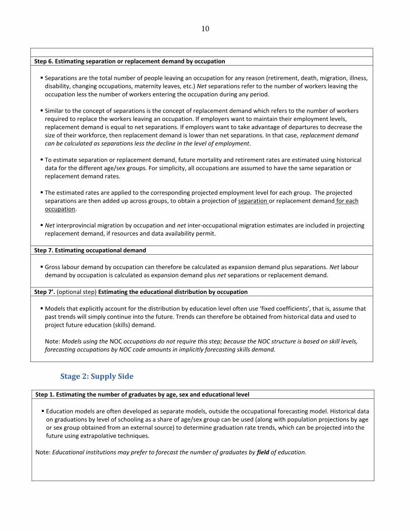
Step 6. Estimating separation or replacement demand by occupation

Separations are the total number of people leaving an occupation for any reason (retirement, death, migration, illness,

disability, changing occupations, maternity leaves, etc.) Net separations refer to the number of workers leaving the occupation less the number of workers entering the occupation during any period.

Similar to the concept of separations is the concept of replacement demand which refers to the number of workers

required to replace the workers leaving an occupation. If employers want to maintain their employment levels, replacement demand is equal to net separations. If employers want to take advantage of departures to decrease the size of their workforce, then replacement demand is lower than net separations. In that case, replacement demand can be calculated as separations less the decline in the level of employment.

To estimate separation or replacement demand, future mortality and retirement rates are estimated using historical

data for the different age/sex groups. For simplicity, all occupations are assumed to have the same separation or replacement demand rates.

The estimated rates are applied to the corresponding projected employment level for each group. The projected

separations are then added up across groups, to obtain a projection of separation or replacement demand for each occupation. Net interprovincial migration by occupation and net inter-occupational migration estimates are included in projecting

replacement demand, if resources and data availability permit.

Step 7. Estimating occupational demand

Gross labour demand by occupation can therefore be calculated as expansion demand plus separations. Net labour

demand by occupation is calculated as expansion demand plus net separations or replacement demand.

Step 7’. (optional step) Estimating the educational distribution by occupation

Models that explicitly account for the distribution by education level often use ‘fixed coefficients’, that is, assume that

past trends will simply continue into the future. Trends can therefore be obtained from historical data and used to project future education (skills) demand. Note: Models using the NOC occupations do not require this step; because the NOC structure is based on skill levels, forecasting occupations by NOC code amounts in implicitly forecasting skills demand.

Stage 2: Supply Side

Step 1. Estimating the number of graduates by age, sex and educational level

Education models are often developed as separate models, outside the occupational forecasting model. Historical data

on graduations by level of schooling as a share of age/sex group can be used (along with population projections by age or sex group obtained from an external source) to determine graduation rate trends, which can be projected into the future using extrapolative techniques.

Note: Educational institutions may prefer to forecast the number of graduates by field of education.

11

Step 2. Estimating the labour force participation and the labour force by age, sex group and educational level

Labour force participation rate trends can be calculated from historical data and projected forward using an

extrapolation technique. The trends are then applied to the corresponding demographic group population projections to obtain the projected labour force for these groups. If graduation trends were estimated, these rates can also be applied to the corresponding labour force estimates

calculated in this step, to obtain estimates of the educated labour force by demographic group. The estimates by age/sex group are then added to obtain an estimate of the projected overall labour force.

Step 3. Including Interprovincial Migration

In sub-national models, inter-regional migration is usually added to the model as an exogenous variable (i.e. changes in

inter-regional migration are assumed to be independent from changes in the other factors determining the size of the labour force). If estimates of interprovincial out-migration were included in the calculation of replacement demand (demand side),

estimates of interprovincial in-migration can be included in the calculation of the labour force (supply side). The number of interprovincial in-migrants is then added to the projected overall labour force from Step 2.

Note: If net interprovincial migration by occupation was included in the calculation of replacement demand, interprovincial in-migrants do not need to be included at this stage. Similarly, inter-occupational migration does not need to be accounted for at this stage because of the inclusion of net inter-occupational migration in estimating replacement demand in the previous stage (demand side). Note: Inter-occupational mobility can be expected to be higher for lower-skill and/or entry level occupations

Step 4. Including Immigration

In some models, such as Canada’s COPS model, the number of immigrants entering an occupation’s labour force are

estimated and included in the model. The number of immigrants by occupation is estimated using the aggregate flow of immigrants into the workforce and fixed occupation shares (the distribution of immigrants by occupation) obtained from census data.

Step. 5 Including Re-entrants

In some models, the number of workers re-entering an occupation’s labour force after a period of non-employment

are estimated and included in the model. Note: this step can be omitted if re-entrants are accounted for in the labour force participation estimates in Step 2.

Step 6. Estimating labour supply by occupation

The occupational labour supply can be estimated by using historical trends of the occupational shares in the labour

force, or by using an education to occupation matrix.

12

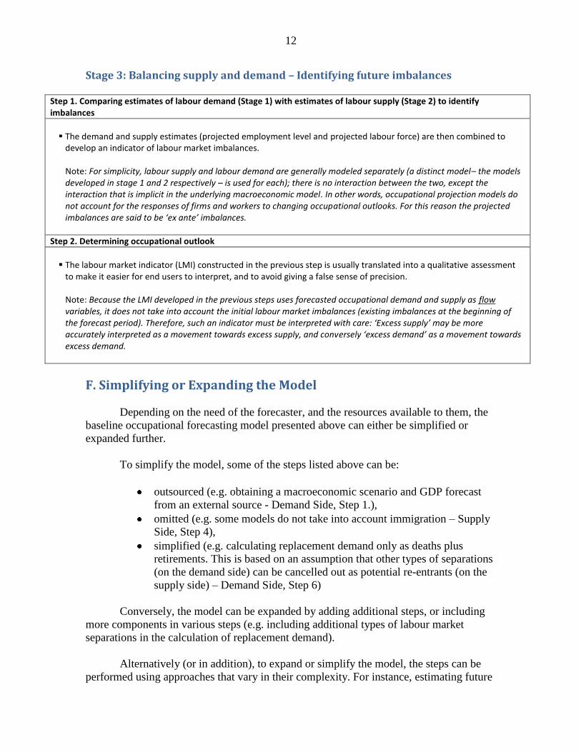
Stage 3: Balancing supply and demand – Identifying future imbalances

Step 1. Comparing estimates of labour demand (Stage 1) with estimates of labour supply (Stage 2) to identify imbalances

The demand and supply estimates (projected employment level and projected labour force) are then combined to

develop an indicator of labour market imbalances. Note: For simplicity, labour supply and labour demand are generally modeled separately (a distinct model– the models developed in stage 1 and 2 respectively – is used for each); there is no interaction between the two, except the interaction that is implicit in the underlying macroeconomic model. In other words, occupational projection models do not account for the responses of firms and workers to changing occupational outlooks. For this reason the projected imbalances are said to be ‘ex ante’ imbalances.

Step 2. Determining occupational outlook

The labour market indicator (LMI) constructed in the previous step is usually translated into a qualitative assessment

to make it easier for end users to interpret, and to avoid giving a false sense of precision.

Note: Because the LMI developed in the previous steps uses forecasted occupational demand and supply as flow variables, it does not take into account the initial labour market imbalances (existing imbalances at the beginning of the forecast period). Therefore, such an indicator must be interpreted with care: ‘Excess supply’ may be more accurately interpreted as a movement towards excess supply, and conversely ‘excess demand’ as a movement towards excess demand.

F. Simplifying or Expanding the Model

Depending on the need of the forecaster, and the resources available to them, the

baseline occupational forecasting model presented above can either be simplified or

expanded further.

To simplify the model, some of the steps listed above can be:

outsourced (e.g. obtaining a macroeconomic scenario and GDP forecast

from an external source - Demand Side, Step 1.),

omitted (e.g. some models do not take into account immigration – Supply

Side, Step 4),

simplified (e.g. calculating replacement demand only as deaths plus

retirements. This is based on an assumption that other types of separations

(on the demand side) can be cancelled out as potential re-entrants (on the

supply side) – Demand Side, Step 6)

Conversely, the model can be expanded by adding additional steps, or including

more components in various steps (e.g. including additional types of labour market

separations in the calculation of replacement demand).

Alternatively (or in addition), to expand or simplify the model, the steps can be

performed using approaches that vary in their complexity. For instance, estimating future

13

employment by occupation based on future industry employment can be done in various

ways, including the following (listed by increasing complexity):

using „fixed coefficients‟ or shares, calculated from historical data. Here

the assumption is that the distribution of occupations by industry does not

change over time.

allowing the coefficients to change over time, based on the historical trend

only.

Estimating the future coefficients or shares by accounting for various

factors that may influence the occupational structure of industries (e.g.

technological change, a change in organizational culture within industries,

etc.).

A challenging but important expansion of the model would be to allow for

demand and supply interactions, or to determine the two simultaneously. Very few

models currently use this approach, due to its complexity and resource intensity. One

notable exception is the Dutch ROA model, briefly outlined in Annex 3.

Another challenging expansion of the model would be to allow for a feedback effect from

occupational demand and supply into the underlying macroeconomic scenario. This may

be relevant for instance in models where the macroeconomic scenario explicitly accounts

for large projects, the completion of which may be dependent on the availability of

labour.

14

IV. Limitations of Occupational Modeling and Forecasting

There are several limitations to occupational modeling and forecasting. First, the

accuracy of these models is a source of concern. To a significant extent, the accuracy of

an occupational model‟s forecasts depends on the soundness of the macroeconomic

scenario on which the model is based. If this underlying macroeconomic forecast is

inaccurate, then the occupational forecast is likely inaccurate as well.

The difficulty of predicting and accounting for the impact of factors such as

technological change (e.g. in terms of labour-capital substitution or new skills demand),

and measuring important concepts such as inter-occupational mobility (or labour-labour

substitution) constitutes a challenge for occupational forecasting. Measurement errors in

these variables and wrong assumptions about them result in inaccurate forecasts. For this

reason, occupational forecasts tend to be more accurate at a higher level of aggregation

(for occupational groups rather than occupations). However, stakeholders and

policymakers are generally more interested in forecasts at lower levels of aggregation.

A related limitation is the simple unavailability of reliable data underlying key

assumptions at detailed levels. For example, COPS uses national 3-digit occupational

data to project provincial 4-digit occupational data on retirements, and it uses only data

on complete labour force withdrawals, ignoring partial labour force withdrawals such as

reductions in hours worked. Given that future demand is in large part driven by

retirements such limitations are not trivial.

The accuracy limitation is even deeper for occupational forecasting than for

traditional forecasting because, unlike most traditional forecasting, occupational forecasts

generally do not include measures of their accuracy. The large number of variables

feeding into these models has made the measurement of accuracy difficult, and little

energy has been spent measuring their past accuracy.4 Given these significant limitations,

even in mainstream models such as COPS, it is important to cross-check results of such

projections with alternate indicators.

Another limitation of most existing occupational forecast models is that they do

not allow for supply and demand interactions, and do not take into account the responses

of workers and firms to changing occupational prospects.5 This limitation is one of the

main differences with traditional forecasting, and it stems in large part from the

somewhat unique purpose of occupational forecasting, which is to inform key

stakeholders whether actions to correct imbalances should be undertaken rather than to

anticipate whether these interventions will take place.

4 Of course, measuring the accuracy of past occupational projections is of limited use given that the models

do not account for supply and demand interactions, and thus are not constructed to be predictors of future

imbalances, but rather to be indicators of future imbalances if no action were to be taken. 5 Projections of occupational shortages or surpluses that do not take into account the inevitability of supply

and demand adjustments are not wrong, they are merely misleading. If supply and demand adjusted

perfectly to every forecast shortage or surplus, no ex ante shortage or surplus would ever be observed ex

post.

15

Finally, occupational models do not differentiate between workers in the same

occupation or skill group who may have different levels of ability, or workers employed

in occupations that do not directly correspond to their formal qualifications.

16

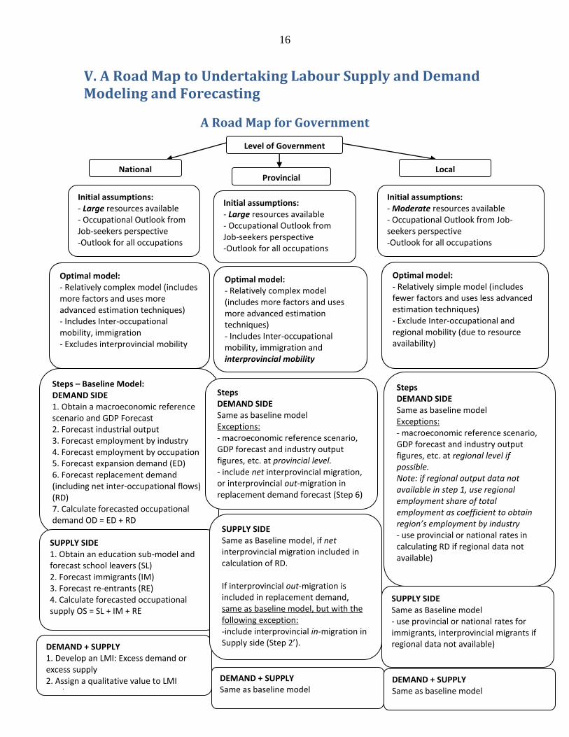
V. A Road Map to Undertaking Labour Supply and Demand Modeling and Forecasting

A Road Map for Government

National Provincial

Level of Government

Local

Initial assumptions: - Large resources available - Occupational Outlook from Job-seekers perspective -Outlook for all occupations

Initial assumptions: - Large resources available - Occupational Outlook from Job-seekers perspective -Outlook for all occupations

Initial assumptions: - Moderate resources available - Occupational Outlook from Job-seekers perspective -Outlook for all occupations

Optimal model: - Relatively complex model (includes more factors and uses more advanced estimation techniques) - Includes Inter-occupational mobility, immigration - Excludes interprovincial mobility

Optimal model: - Relatively complex model (includes more factors and uses more advanced estimation techniques) - Includes Inter-occupational mobility, immigration and interprovincial mobility

Optimal model: - Relatively simple model (includes fewer factors and uses less advanced estimation techniques) - Exclude Inter-occupational and regional mobility (due to resource availability)

Steps – Baseline Model: DEMAND SIDE 1. Obtain a macroeconomic reference scenario and GDP Forecast 2. Forecast industrial output 3. Forecast employment by industry 4. Forecast employment by occupation 5. Forecast expansion demand (ED) 6. Forecast replacement demand (including net inter-occupational flows) (RD) 7. Calculate forecasted occupational demand OD = ED + RD

SUPPLY SIDE 1. Obtain an education sub-model and forecast school leavers (SL) 2. Forecast immigrants (IM) 3. Forecast re-entrants (RE) 4. Calculate forecasted occupational supply OS = SL + IM + RE

DEMAND + SUPPLY 1. Develop an LMI: Excess demand or excess supply 2. Assign a qualitative value to LMI results

Steps DEMAND SIDE Same as baseline model Exceptions: - macroeconomic reference scenario, GDP forecast and industry output figures, etc. at provincial level. - include net interprovincial migration, or interprovincial out-migration in replacement demand forecast (Step 6)

SUPPLY SIDE Same as Baseline model, if net interprovincial migration included in calculation of RD. If interprovincial out-migration is included in replacement demand, same as baseline model, but with the following exception: -include interprovincial in-migration in Supply side (Step 2’).

DEMAND + SUPPLY Same as baseline model

Steps DEMAND SIDE Same as baseline model Exceptions: - macroeconomic reference scenario, GDP forecast and industry output figures, etc. at regional level if possible. Note: if regional output data not available in step 1, use regional employment share of total employment as coefficient to obtain region’s employment by industry - use provincial or national rates in calculating RD if regional data not available)

SUPPLY SIDE Same as Baseline model - use provincial or national rates for immigrants, interprovincial migrants if regional data not available)

DEMAND + SUPPLY Same as baseline model

17

A Road Map for Educational Institutions

Education Ministry University/ College

Educational Institution

Vocational/Specialized Training Institution

Initial assumptions: - Large resources available - Skills/ qualifications forecast -Forecast for all skills - Perspective of students

Initial assumptions: - Low-Moderate resources available - Forecast for all skills - Perspective of students -Outlook for all occupations

Initial assumptions: - Low-Moderate resources available -Forecast for all skills - Perspective of students

Optimal model: - Relatively Complex model (includes more factors and uses more advanced estimation techniques) - Includes Inter-occupational mobility, immigration - Excludes interprovincial mobility

Optimal model: - Relatively simple model (includes fewer factors and uses less advanced estimation techniques)

Optimal model: - Relatively simple model (includes fewer factors and uses less advanced estimation techniques) - Education sub-model developed in-house (using vocational training data)

Steps – Baseline Model: DEMAND SIDE 1. Obtain a macroeconomic reference scenario and GDP Forecast 2. Forecast industrial output 3. Forecast employment by industry 4. Forecast employment by occupation 5. Forecast expansion demand (ED) 6. Forecast replacement demand (including net inter-occupational flows) (RD) 7. Calculate forecasted occupational demand OD = ED + RD 8. Forecast immigrants and re-entrants by occupation (IM+RE) 9. Calculate demand to be filled by education system as OD’ = OD - (IM +RE) 9. Use educational outcome matrix to translate OD’ into demand for skills/by field of study

SUPPLY SIDE 1. Obtain school leavers by skill level/ field of education from external source: Skills supply (OS’)

DEMAND + SUPPLY 1. Develop a skills gap indicator: OD’ – OS’ 2. Assign a qualitative value to indicator results

Steps DEMAND SIDE Same as baseline model, using less advanced estimation techniques

SUPPLY SIDE Same as baseline model

DEMAND + SUPPLY Same as baseline model

DEMAND SIDE Same as baseline model, but first identifying relevant industry/sector and relevant occupations and obtaining all data and forecasts for these industries/ occupations only.

SUPPLY SIDE Forecast Skills supply (OS’) using historical vocational training data (enrolment, completion rates, length of programs)

DEMAND + SUPPLY Same as baseline model

18

A Road Map for Industry

Sector Councils/ Associations Unions

Industry

Companies (employers)

Initial assumptions: - Moderate-Large resources available - Occupational Outlook from employers’ perspective -Outlook for sector’s occupations

Initial assumptions: - Low-Moderate resources available - Occupational Outlook from workers’ perspective -Outlook for members’ occupations

Initial assumptions: - Low-Moderate resources available - Occupational Outlook from employers’ perspective --Outlook for sector’s occupations Optimal model:

- Relatively Complex model (includes more factors and uses more advanced estimation techniques) - Includes Inter-occupational mobility and immigration

Optimal model: - Relatively simple model (includes fewer factors and uses less advanced estimation techniques) - Includes Inter-occupational mobility and immigration

Optimal model: - Relatively simple model (includes fewer factors and uses less advanced estimation techniques)

Steps – Baseline Model: DEMAND SIDE 1. Obtain macroeconomic reference scenario and GDP forecast 2. Identify relevant industry/sector and relevant occupations 3. Forecast industrial output for relevant industry/sector 4. Forecast employment by industry 5. Forecast employment by occupation 6. Forecast expansion demand (ED) 7. Forecast replacement demand (including net inter-occupational flows) (RD) 8. Calculate forecasted occupational demand as OD = ED + RD

SUPPLY SIDE 1. Obtain an education sub-model and forecast school leavers (SL) 2. Forecast immigrants (IM) 3. Forecast re-entrants (RE) 4. Calculate forecasted occupational supply OS = SL + IM + RE

DEMAND + SUPPLY 1. Develop an LMI: Excess demand or excess supply 2. Assign a qualitative indicator based on LMI. Outlook from employer’s perspective: Good if excess supply, bad if excess demand

Steps DEMAND SIDE Same as baseline model, using less advanced estimation techniques

SUPPLY SIDE Same as baseline model

DEMAND + SUPPLY Same as baseline model, exception: Assign a qualitative indicator based on LMI. Outlook from workers’ perspective: Good if excess demand, bad if excess supply

Steps DEMAND SIDE Same as baseline model, using less advanced estimation techniques

SUPPLY SIDE Same as baseline model, using less advanced estimation techniques

SUPPLY SIDE Same as baseline model

19

Bibliography

Boothby, D. (1995a) “COPS: A Revised Demand Side,” Human Resources Development

Canada, Applied Research Branch, Strategic Policy, Technical Document T-95-4, June.

Boothby, D. (1995b) “COPS: A Revised Supply Side,” Human Resources Development

Canada, Applied Research Branch, Strategic Policy, Technical Document T-95-5, July.

Boydell, K., Gauthier J. and Hughes K. (1995), “COPS: A New Model for Occupational

Coefficients,” Human Resources Development Canada, Applied Research Branch,

Strategic Policy, Technical Document T-95-6, July.

Canadian Council on Learning (2007) „Is it possible to accurately forecast Labour Market

Needs?‟ prepared for the British Columbia Ministry of Advanced Education, January.

Centre for Spatial Economics (2005) “Literature Review on Estimating Inter-

occupational Labour Mobility in a Federal, Provincial and Territorial Environment”

prepared for the Forum of Labour Market Ministers, Labour Market Information Group,

March.

Centre for Spatial Economics (2006) “Consultations on Enhancing Canada‟s Labour

Market Supply Modeling Capacity at Provincial-Territorial Level: Recommendations

Report” prepared for the Forum of Labour Market Ministers, Labour Market Information

Group, March.

Centre for Spatial Economics (2008) “Future Labour supply and Demand 101: A Guide

to Analysing and Predicting Occupational Trends”, prepared for the Forum of Labour

Market Ministers, Labour Market Information Working Group, March.

Employment and Immigration Alberta (2009) „Alberta‟s Occupational Demand and

supply Outlook, 2008-2018‟, available at

http://employment.alberta.ca/cps/rde/xchg/hre/hs.xsl/2656.html

Foot, D. and Meltz N. (1992) "An Ex Post Evaluation of Canadian Occupational

Projections, 1961-1981,” Relations Industrielles/Industrial Relations, Vol. 47, No. 2, pp.

200-211.

Henson, H. and Newton C. (1996) “Tools and Methods for Identifying Skill Shortages: A

Cross-Country Comparison,” Human Resources Development Canada, Applied Research

Branch, Strategic Policy, Technical Document T-96-3E.

Herzog, D. (2007) “Labour Supply Monitoring and Forecasting Workshop, Summary

Report,” prepared for the Forum of Labour Market Ministers, Labour Market Information

Group, October.

20

Infometrica Limited (1996) “COPS 1996 Macroeconomic Reference Scenario,” Human

Resources Development Canada, Applied Research Branch, Strategic Policy, Technical

Document T-96-1E, January.

Meltz, N. (1996) “Occupational Forecasting in Canada: Back to the Future,” Human

Resources Development Canada, Applied Research Branch, Strategic Policy, Technical

Document T-96-4E, June.

Smith, D. (2002) “Forecasting future skill needs in Canada,” in Forecasting Labour

Markets in OECD Countries: Measuring and Tackling Mismatches, Ed. Michael Neugart

and Klaus Schömann Edward Elgar,

http://books.google.ca/books?id=cdgrcJLlPoYC&dq=accuracy+of+occupational+forecast

ing+oecd&source=gbs_summary_s&cad=0.

Roth, W. (1995) “Canadian Occupational Projection System: A Presentation of Results

using a Revised Framework,” Human Resources Development Canada, Applied Research

Branch, Strategic Policy, Technical Document T-95-3.

21

Annex 1 – Glossary of Basic Terminology Aggregate Labour Shortage: occurs when there is (near) full employment and a general

difficulty in finding workers to fill vacancies.

Cobweb Cycle: situation arising when students base their educational decisions on the market at

the time they enter a course, rather than the market anticipated at their time of graduation. The

cobweb model developed by Kaldor was first used to describe and explore the relationship

between educational choice, wages and labour market outcomes by Richard Freeman in a series

of articles.

Employment: the number of people working in all industries, in an industry or occupation.

Employment Rate (Employment-to-population ratio): the number of working people in all

industries, in an industry or occupation (employment) as a percentage of the total population.

Flow (or Flow Variable): measure of the change in stock or stock variable (change in a quantity

over a period of time).

Quality Gap: when there are sufficient people with the essential technical skills, not already

using them, who are willing to apply for the vacancies, but who lack other qualities that

employers think are important.

Labour Force: the number of people available for work in all industries, or in a specific industry

or occupation.

Labour Force Participation Rate: the number of people available to work (labour force) in all

industries, in an industry or an occupation, as a percentage of the total population.

Labour Market Adjustment: shift in labour demand and/or labour supply towards an

equilibrium (to offset an imbalance).

Labour Market Equilibrium: a situation where labour supply and demand are equal given a set

of labour market conditions.

Labour Market Mismatch: has four basic sub-types:

Qualitative mismatch: occurs when the qualifications of workers and the qualification

needed to fill available vacancies are not matched. Can also be referred to as „skills

mismatch.‟ Is sometimes referred to as „skills shortage.‟

Regional mismatch: occurs when the unemployed persons seeking work and firms offering

suitable jobs are located in different regions, and the jobs and/or workers are immobile.

Preference mismatch: refers to a mismatch between the types of jobs that unemployed

people are willing to take on, and existing vacancies in the relevant region. Those out of work

are unwilling to take certain types of work because of inadequate remuneration or working

conditions or status, despite the fact that such jobs match their qualifications and skills profile,

or are located in the relevant geographical region.

Information mismatch: occurs when unemployed workers do not acquire information on

relevant existing vacancies, and firms do not have the information necessary for finding

persons with adequate qualifications. Supply does not meet demand because of the lack of

information.

22

Labour Shortage (or Excess Demand): occurs when the demand for workers for a particular

occupation is greater than the supply of workers who are qualified, available and willing to work

under existing market conditions.

Labour Surplus (or Excess Supply): occurs when the supply of workers who are qualified,

available and willing to work in a particular occupation is greater than the demand for workers

under existing market conditions.

Occupation Coefficient: share of employment in an industry accounted for by each occupation.

Skill Shortage or Skill Gap: a divergence between the quantity of a given skill supplied by the workforce and the

quantity demanded by employers under the existing market conditions (given the existing

level of compensation and wage structure).

a situation in which employers are hiring workers whom they consider under-skilled or in

which their existing workforce is under-skilled relative to some desired level.

a labour market situation in which there is a lack of people with the qualifications, skills

or experience necessary to carry out the jobs in question. Sometimes referred to as

„qualitative skills mismatch.‟

Stock (or Stock Variable): a fixed measure at a point in time. Changes in stocks are „flows.‟

Unemployment: the number of workers who are available to work (in the labour force) but who

are not working. Unemployment is calculated as the labour force less employment.

Unemployment Rate: Unemployed people as a percentage of the labour force.

Natural Rate of Unemployment: a level of joblessness that is warranted even where the

market is working 'ideally' because, for example, of the need for workers to look for new

jobs or because of the random and unforeseen shocks to the economic system to which

adjustment needs to be made. The natural rate of unemployment (NRU) was also

originally identified as that point at which inflation would not accelerate or decelerate,

along the vertical part of the Phillips curve. The persistence of unemployment and

inflation in the 1980s led to the notion of the non-accelerating inflation rate of

unemployment (NAIRU).

23

Annex 2 – A List of Additional Resources

Websites

Construction Sector Council (CSC) forecasts: www.constructionforecasts.ca/forecasts

Emploi-Quebec: http://emploiquebec.net/

FLMM: http://www.flmm-lmi.org/

Service Canada: http://www.servicecanada.gc.ca/

Government of Alberta, Employment and Immigration, Labour Market Forecasts:

http://employment.alberta.ca/BI/2656.html

Labour Market & Career Information for Newfoundland and Labrador: LMIworks:

http://www.lmiworks.nl.ca/LMIToolkit/Default.aspx

Statistics Canada:

http://www40.statcan.gc.ca/l01/ind01/l3_2621-eng.htm?hili_none

Publications Construction Sector Council, Construction Looking Forward

Employment and Immigration Alberta (2009) „Alberta‟s Occupational Demand and

supply Outlook, 2008-2018‟, available at

http://employment.alberta.ca/cps/rde/xchg/hre/hs.xsl/2656.html

Human Resources and Social Development Canada, Looking-Ahead: A 10-Year Outlook

for the Canadian Labour Market (2006-2015), available at

http://www.hrsdc.gc.ca/eng/publications_resources/research/categories/labour_market_e/

sp_615_10_06/page00.shtml

Canadian Data Sources

LMI data works: http://www.lmiworks.nl.ca:8080/webview/

Contains data by topic (Population, Labour Force, Education, Employment, Income), by

geography (Canada, Provinces, and Territories, Rural regions, economic zones,

CMAÉCAs and non CMAÉCAs, and communities) and by source (LFS, Census,

Taxfiler).

24

Annex 3 – Examples of Occupational Forecasting Models

A. Canadian COPS model

The Canadian Occupational Projection System (COPS) model, developed by Human

Resources and Skills Development Canada (HRSDC), produces occupational outlooks

based on the NOC system. The COPS model was originally an occupational demand

model, but was extended since the mid 1990s to include supply side information (Centre

for Spatial Economics, 2005: 84).

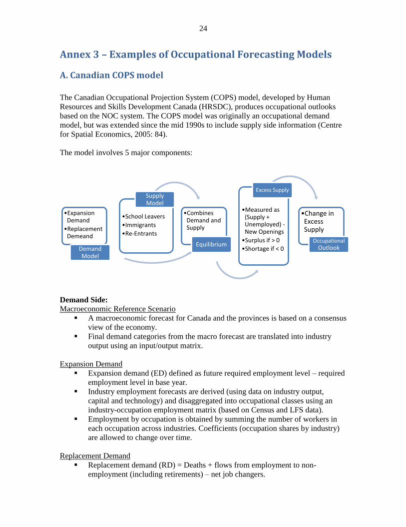
The model involves 5 major components:

Demand Side:

Macroeconomic Reference Scenario

A macroeconomic forecast for Canada and the provinces is based on a consensus

view of the economy.

Final demand categories from the macro forecast are translated into industry

output using an input/output matrix.

Expansion Demand

Expansion demand (ED) defined as future required employment level – required

employment level in base year.

Industry employment forecasts are derived (using data on industry output,

capital and technology) and disaggregated into occupational classes using an

industry-occupation employment matrix (based on Census and LFS data).

Employment by occupation is obtained by summing the number of workers in

each occupation across industries. Coefficients (occupation shares by industry)

are allowed to change over time.

Replacement Demand

Replacement demand (RD) = Deaths + flows from employment to non-

employment (including retirements) – net job changers.

•Expansion Demand

•Replacement Demeand

Demand Model

•School Leavers

•Immigrants

•Re-Entrants

Supply Model

•Combines Demand and Supply

Equilibrium

•Measured as (Supply + Unemployed) -New Openings

•Surplus if > 0

•Shortage if < 0

Excess Supply

•Change in Excess Supply

Occupational Outlook

25

A simple regression model of replacement demand as a proportion of required

employment is estimated. The model is then used to project this proportion into

the future. The projected proportion is multiplied by the projected employment

requirement by occupation to obtain the projected level of replacement demand.

Attrition rates used in this model are not occupation-specific: death rates are

obtained by using mortality rates by age/gender and applying them to

corresponding groups. Withdrawal rates for other reasons are estimated as

changes in participation rates by group.

Occupational Demand

New openings = ED + RD

Supply Side:

Education Component (School Leavers):

An education sub-model projects the number of graduates in a given year. The

model uses historical data to calculate enrolment rates by age/gender for 6 levels

of schooling. Trends in he historical rates are then used to project future rates,

which are applied to the corresponding population groups. To obtain the number

of graduates for the forecast year, a fixed proportion (the last observed

proportion) is applied to the enrolment numbers of the year when graduates

would have normally entered the program (e.g. for a four-year program, the

projected number of graduates in 2010 is obtained by applying the fixed

graduation rate (last observed) to the enrolment numbers in 2006). A similar

process is used to estimate dropouts. Dropouts for each level are considered as

graduates of the next lowest level.

A transition matrix of field-of-study to occupation is used to convert data on

projected graduates by level of education and field of study into projected

entrants in the occupation labour force.

Immigrants

Immigration numbers are determined for the initial year of the projection, based

on the federal government‟s announced quota and assumed to be constant over

the forecast period.

Occupational distribution is determined using a Statistics Canada survey that

identifies the occupations where immigrants work.

Potential Re-entrants

The trend (adjusted for the business cycle) in historical data of the flow from

employment to non-employment, expressed as a proportion of employment, is

obtained from a simple regression model. The model is then used to project this

proportion into the future. The projected proportion is then applied to the

projected employment figures to obtain the projected number of potential re-

entrants.

26

Occupational Supply

Occupational supply = school leavers + immigrants + re-entrants

Demand and Supply:

LMI Indicators

Excess Supply = (Occupational Supply + Unemployed) – New Openings

Outlook/Qualitative Assessment:

Change in Excess Supply

Surplus if > 0, Shortage if < 0

The labour market outlook from the job-seeker‟s perspective is qualified as „good‟, „fair‟

or „limited.‟

B. BC Education Model

A large and detailed dataset is constructed using data on student records at the

secondary and post-secondary level is prepared, educational programs are coded

by 6-digit Classification of Instructional Program (CIP) level and further divided

into length of program. The stock of BC students by current level of schooling is

then projected into the future.

BC Colleges and Universities Outcome Survey data are then used to transform

the projected number of students by education to the number of potential

workers by occupation (transition from CIP to 4-digit NOC).

C. Alberta Occupational Demand and Supply Outlook Models

Alberta Employment and Immigration has developed the Alberta Occupational Demand

Outlook Model (AODOM) and the Alberta Occupational Supply Outlook Model

(AOSOM). Each of the models is linked to a number of sub-models.

Demand Side:

Expansion Demand:

An industry employment forecast is made based on a macroeconomic forecast, a

forecast of output by industry and accounting for the changing employment

structure of industries.

Employment by industry is translated into employment by occupation.

Replacement Demand:

Retirement rates and other separations are derived from the Alberta Labour

Force Survey at an aggregate occupational level.

Separation rates are assumed constant over the forecast period, with the

exception of retirement rates which are assumed to rise over time, based on the

age distribution by occupation (obtained from Census data).

27

Emigration, out-migration and death rates by age/gender group are assumed to

be the same for the general population.

Occupational Demand

New openings = ED + RD

Supply Side:

Population/Demographic Component:

Population levels by age and gender groups are projected by single year cohort.

Net-migration by age and gender is projected using historical trends. In-

migration is calculated as projected net-migration plus assumed out-migration.

Future immigrants are assumed to face similar occupational outcomes as

existing residents of the province.

Alberta‟s aboriginal population is assumed to have the same birth and mortality

rates as the Canadian aboriginal population.

Alberta‟s visible minorities‟ birth and mortality rates are assumed equal to

Alberta‟s general population birth and mortality rates.

A method is used to account for the population with activities limitations.

Education Component:

Secondary and post-secondary school enrolment rates are assumed to follow

historical trends.

Graduation rates are calculated by level of schooling, field of study, age and

gender, and kept constant over the forecast period.

Drop out rates and mature student rates are calculated by level and field of

study.

Migration rates by educational attainment are adjusted to reflect demand

conditions in the province.

Educational attainment is projected by field of study.

Occupational Supply:

Potential occupational supply is determined by using the historical distribution

of occupation by educational attainment.

Actual occupational supply is determined by using historical participation rates

by occupation.

Demand and Supply:

LMI Indicators

A measure of labour market imbalances is calculated as the ratio of projected labour

demand over projected labour supply.

Outlook/Qualitative Assessment:

Labour Market balance if ratio = 1, Potential shortage if ratio > 1, potential labour surplus

if ratio < 1.

28

Note: In the updated version of the model, demand and supply are allowed to interact. In

particular, changes in demand affect the coefficients of occupation by education.

D. Construction Sector Council Model

The Construction Sector Council (CSC) model provides an outlook for over 30

construction trades, for each of the Canadian provinces and for the Ontario regions.

Demand Side:

Macroeconomic Reference Scenario:

A macroeconomic scenario is prepared, which takes into account building

requirements related to construction projects (large and small, announced and

unannounced), maintenance and repair construction activities.

Expansion Demand:

Investment and employment forecasts are combined with a set of coefficients to

forecast labour requirements by trade. Coefficients used often vary depending on

the major projects included in the macroeconomic forecast, because different

projects differ in their trades requirements.

Forecasted labour demand by trade includes demand by the construction sector,

and by all other sectors that employ trades workers.

Replacement Demand:

Replacement demand is calculated as the number of retirements. Retirements are

estimated using data on mortality rates and changes in labour force participation

for workers over 55 years of age.

Occupational Demand:

Expansion demand and replacement demand are combined to obtain the required

labour requirements by trade for construction and other industries.

Supply Side:

Education (Apprenticeship) Component:

The number of graduates from apprenticeship programs is used, with data on the labour

force by age group, to determine the available labour force by trade.

Immigrants:

Immigrants, aboriginals, women and youth are included in the initial calculation of the

population available to enrol in training/apprenticeship.

Re-entrants:

The number of people entering the labour market after a period of non-participation are

also included on the supply side.

29

Mobility:

The available labour force is adjusted for the mobility or workers across sector, industry

and region.

Occupational Supply:

The occupational supply is calculated from population and training/apprenticeship data

and from population data.

Demand and Supply:

LMI Indicators:

Because of the nature of construction activity, the CSC model calculates three

unemployment rates: the annual rate of unemployment (which eliminates seasonal

variation), the peak rate of unemployment (which accounts for cyclical variation) and the

natural rate of unemployment.

Outlook/Qualitative Assessment:

The CSC model provides a „Labour Market Ranking‟, ranging from 1 (excess supply) to

5 (excess demand).

E. Dutch ROA Model

The ROA model uses two econometric models to produce labour and demand forecasts

for 127 occupational groups and 104 educational types.

Demand Side

Macroeconomic Reference Scenario

Sectoral employment forecasts are produced by the Dutch Central Planning Bureau

(CPB).

Expansion Demand (ED)

Expansion demand is broken down by industrial sectors, occupations and type of

education. Changes in occupational structure derived from a random coefficient approach

using LFS data.

Additional step: Accounts for substitution effects („switching jobs‟) per type of

education.

Replacement Demand (RD)

Replacement demand is calculated by type of education, age and gender as expected

outflow (deaths, retirements, etc.) of workers out of the labour force.

Due to absence of flow data, net inflows or outflows are calculated as changes in stock

data.

Future net outflow rates are calculated from historical rates and adjusted for business

cycle fluctuations.

30

Finally, future net outflow rates by age/gender are combined with population group

projections for each occupation or education category to obtain future RD.

Occupational Demand

Recruitment demand = all job openings (ED + RD)

Supply Side

School Leavers

Educational forecasts of the flow of school levers by age and gender from formal (full-

time and part-time) education system prepared by the education ministry, at an aggregate

level.

ROA provides more detailed forecasts by using a matrix of full-time education and

educational attainment, and projects the number of students by educational category.

Occupational Supply

Data on new supply by education are translated into new supply by occupation using data

about newcomers from the „education accounts‟ of Statistics Netherlands.

Demand and Supply

LMI Indicators

Labour Gap Indicator (LGI): Labour demand (ED+RD+ passive substitution effects) –

Labour supply (expected new supply + number of people unemployed for less than a year

with same educational background).

Outlook/Qualitative Assessment

Based on LGI, prospects for newcomers are characterized as „good‟, „reasonable‟,

„moderate‟ or „poor‟.