a cognitive bias approach to feature selection and weighting for case-based learners

Machine Learning, 41, 85–116, 2000c© 2000 Kluwer Academic Publishers. Manufactured in The Netherlands.

A Cognitive Bias Approach to Feature Selectionand Weighting for Case-Based Learners

CLAIRE CARDIE [email protected] of Computer Science, Cornell University, Ithaca, NY 14853–7501, USA

Editor: David W. Aha

Abstract. Research in psychology, psycholinguistics, and cognitive science has discovered and examined nu-merous psychological constraints on human information processing. Short term memory limitations, a focus ofattention bias, and a preference for the use of temporally recent information are three examples. This paper showsthat psychological constraints such as these can be used effectively as domain-independent sources of bias to guidefeature set selection and weighting for case-based learning algorithms.

We first show that cognitive biases can be automatically and explicitly encoded into the baseline instancerepresentation: each bias modifies the representation by changing features, deleting features, or modifying featureweights. Next, we investigate the related problems of cognitive bias selection and cognitive bias interaction forthe feature weighting approach. In particular, we compare two cross-validation algorithms for bias selection thatmake different assumptions about the independence of individual component biases. In evaluations on four naturallanguage learning tasks, we show that the bias selection algorithms can determine which cognitive bias or biasesare relevant for each learning task and that the accuracy of the case-based learning algorithm improves significantlywhen the selected bias(es) are incorporated into the baseline instance representation.

Keywords: case-based learning, instance-based learning, feature set selection, feature weighting, naturallanguage learning

1. Introduction

Inductive concept acquisition has always been a primary interest for researchers in the fieldof machine learning (Langley, 1996; Mitchell, 1997). Independently, psychologists, psy-cholinguists, and cognitive scientists have examined the effects of numerous psychologicallimitations on human information processing (Wilson & Keil, 1999). However, despite thefact that concept learning is a basic cognitive task, cognitive processing limitations arerarely exploited in the design of machine learning systems for concept acquisition.

This paper shows that cognitive processing limitations can be used effectively as domain-independent sources of bias to guide feature set selection and, as a result, to improvelearning algorithm performance. We first describe how cognitive biases can be automati-cally and explicitly encoded into a training instance representation. In particular, we usea simple case-based learning algorithm (k-nearest neighbor (Cover & Hart, 1967)) andinitially focus on a single learning task from the field of natural language processing.

86 C. CARDIE

After presenting a baseline instance representation for the task, we modify the represen-tation in response to three cognitive biases—a focus of attention bias (Broadbent, 1958),a recency bias (Kimball, 1973), and short term memory limitations (Miller, 1956). In aseries of experiments, we compare the modified instance representations to the baselinedescription and find that, when used in isolation, only one cognitive bias significantly im-proves system performance. We hypothesize that additional gains in accuracy might beachieved by applying two or more cognitive biases simultaneously to the baseline instancerepresentation.

As more psychological processing limitations are included in the instance representa-tion, however, the system must address the related issues of cognitive bias interaction andcognitive bias selection. As a result, the paper next presents two methods for cognitive biasselection that make varying assumptions about the independence of individual processinglimitations. In general, each method combines search and cross validation. The greedyapproach to bias selection incrementally incorporates into the baseline representation thebest-performing individual cognitive biases while the learning algorithm’s accuracy con-tinues to improve. This method assumes that there will be few deleterious bias interactions.In contrast, the second algorithm for bias selection makes no assumptions about bias in-teractions and instead exhaustively evaluates all combinations of the available cognitivebiases. Our work differs from most previous work in that we use search and cross validationfor bias selection rather than for feature selection; the selected biases are then responsiblefor directing feature set selection and feature weighting. The results of our experimentsshow that the bias selection algorithms can determine which cognitive biases are relevantfor each learning task and that performance of the case-based learning algorithm improvessignificantly when the selected bias or biases are incorporated into the baseline instancerepresentation.

Finally, we investigate the generality of the cognitive bias approach to feature set selection.We first show that two additional cognitive biases can be translated into representationalchanges for the baseline instance representation. We then apply the feature selection al-gorithm with all five cognitive biases to three additional natural language learning tasks.Again, we find that (1) the cognitive bias selection algorithms are able to choose one ormore appropriate biases for each task, and (2) the incorporation of these relevant biasessignificantly improves the learning algorithm’s performance.

The remainder of the paper is organized as follows. The next two sections describe the firstnatural language learning task—relative pronoun disambiguation—and its baseline instancerepresentation. This task will be used throughout the paper to introduce components of thecognitive bias approach to feature set selection. Section 4 presents the case-based learningalgorithm and its evaluation on the relative pronoun task. The method used to incorporateindependently each of the three primary cognitive biases—focus of attention, recency,short term memory limitations—is described in Section 5. Section 6 proposes and evaluatesthe alternative approaches to bias selection briefly outlined above. An evaluation of thecognitive bias approach to feature set selection on additional data sets comprises Section 7.Cardie (1999) describes the implications of this work for natural language processing ratherthan machine learning.

A COGNITIVE BIAS APPROACH TO FEATURE SELECTION 87

2. Relative pronoun disambiguation

The goal of the machine learning algorithm for the first natural language task is to disam-biguate wh-words (e.g., who, which, where) in sentences like:

Tony sawthe boywho won the award.

In particular, the learning algorithm must locate the phrase or phrases, if any, that representthe antecedent of the wh-word given a description of the context in which the wh-wordoccurs. For the sample sentence, the system should recognize that “the boy” is the antecedentof “who” because “who” refers to “the boy.” Finding the antecedents of relative pronounsis a crucial task for natural language understanding systems in part because the antecedentfills a semantic role in two clauses. In the sample sentence, for example, “the boy” is boththe object of “saw”and the implicit actor of “won.”

In addition, we focus on disambiguation of relative pronouns because (1) they occurfrequently in the long, multi-clause sentences of many real-world texts, (2) disambiguationof relative pronouns was determined to be critical for the larger information extraction taskwithin which the learning algorithm was embedded, (3) our existing natural language pro-cessing (NLP) system (Lehnert et al., 1991) included hand-crafted disambiguation heuristicswith which we could directly compare the learning algorithm performance, and (4) thereis a large body of literature on the human processing of relative clauses. (Both the cor-pus and the broader information extraction task will be described in Section 3.) We focusmore specifically on learning disambiguation heuristics for “who” because this was themost frequent relative pronoun to appear in the corpus, occurring in about one out of everyten sentences and at a higher frequency for the most important documents, i.e., for textsthat are actually relevant to the information extraction task. In addition, the majority ofpsycholinguistic studies of human processing of relative clauses focus on “who.”

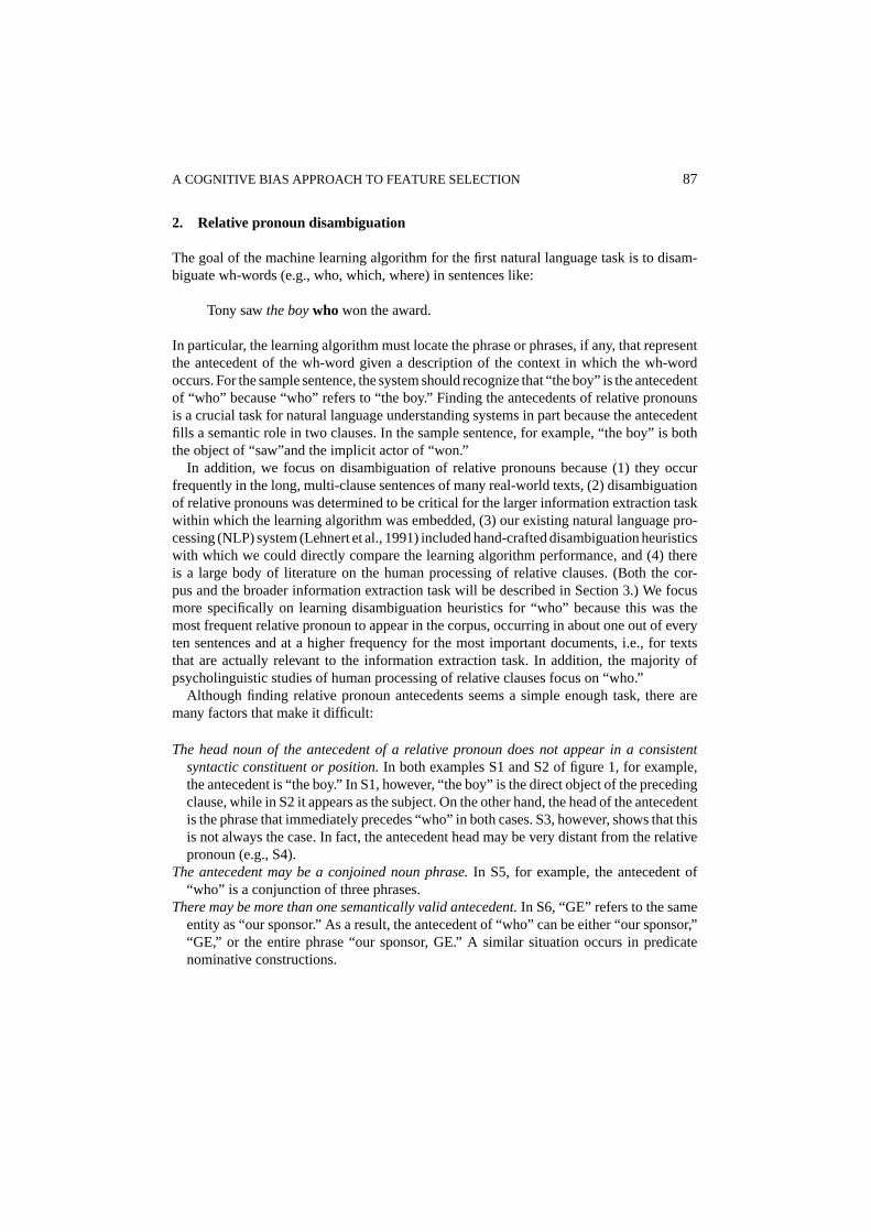
Although finding relative pronoun antecedents seems a simple enough task, there aremany factors that make it difficult:

The head noun of the antecedent of a relative pronoun does not appear in a consistentsyntactic constituent or position.In both examples S1 and S2 of figure 1, for example,the antecedent is “the boy.” In S1, however, “the boy” is the direct object of the precedingclause, while in S2 it appears as the subject. On the other hand, the head of the antecedentis the phrase that immediately precedes “who” in both cases. S3, however, shows that thisis not always the case. In fact, the antecedent head may be very distant from the relativepronoun (e.g., S4).

The antecedent may be a conjoined noun phrase.In S5, for example, the antecedent of“who” is a conjunction of three phrases.

There may be more than one semantically valid antecedent.In S6, “GE” refers to the sameentity as “our sponsor.” As a result, the antecedent of “who” can be either “our sponsor,”“GE,” or the entire phrase “our sponsor, GE.” A similar situation occurs in predicatenominative constructions.

88 C. CARDIE

S1. Tony sawthe boywho won the award.S2. The boywho gave me the book had red hair.S3. Tony ate dinner withthe menfrom Detroitwho sold computers.S4. I spoke tothe womanwith the black shirt and green hat over in the far corner of

the roomwho wanted a second interview.S5. I’d like to thankJim, Terry, and Shawn, who provided the desserts.S6. I’d like to thankour sponsor, GE, who provided financial support.S7. We wonderedwho stole the watch.S8. The womanfrom Philadelphiawho played soccer was my sister.S9. The gifts fromthe childrenwho attended the party are on the table.

Figure 1. Antecedents of “who”.

Sometimes there is no apparent antecedent.As in S7, sentence analyzers must be able todistinguish uses of “who” that have no antecedent (e.g., interrogatives) from instances oftrue relative pronouns.

Locating the antecedent requires the assimilation of both syntactic and semantic knowledge.The syntactic structure of the clause preceding “who” in sentences S8 and S9, for example,is identical. The antecedent in each case is different, however. In S8, the antecedent isthe subject, “the woman.” In S9, it is the head noun of the prepositional phrase, i.e., “thechildren.”

Despite these difficulties, we will show that a machine learning system can learn to locatethe antecedent of “who” given a description of the clause that precedes it.

3. The baseline instance representation

In all experiments, we use the CIRCUS sentence analyzer (Lehnert, 1990) to generatetraining instances. The system generates one instance for every occurrence of “who” thatappears in texts taken from the MUC terrorism corpus. This corpus was developed in con-junction with the third Message Understanding Conference (MUC-3, 1991), a performanceevaluation of state-of-the-art information extraction systems. In general, an information ex-traction system takes as input an unrestricted text and “summarizes” the text with respect toa prespecified topic or domain of interest: it finds useful information about the domain andencodes that information in a structured, template format, suitable for populating databases(Cardie, 1997). The CIRCUS system has been a consistently strong performer in the MUCevaluations. The MUC collection consists of 1300 documents including newswire stories,speeches, radio and TV broadcasts, interviews, and rebel communiques. Texts contain bothwell-formed and ungrammatical sentences; all texts are entirely in upper case.

Each training instance for the relative pronoun task is a list of attribute-value pairs thatencode the context in which the wh-word is found. In addition, each training instance is alsoannotated with a class value that describes the position of the correct antecedent for “who”in each example. This antecedent class value is the feature to be predicted by the learningalgorithm during testing. The details of the baseline instance representation depend, in part,


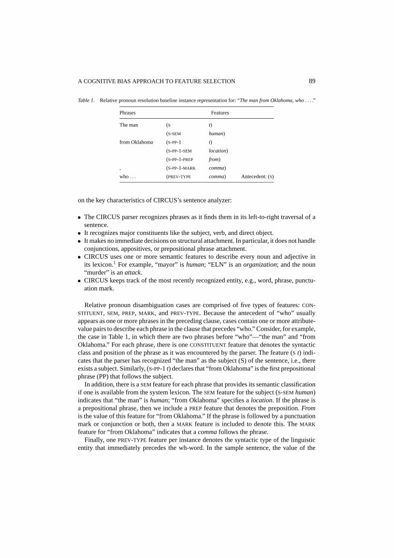
Table 1. Relative pronoun resolution baseline instance representation for: “The man from Oklahoma, who. . . .”

Phrases Features

The man (S t)

(S-SEM human)

from Oklahoma (S-PP-1 t)

(S-PP-1-SEM location)

(S-PP-1-PREP from)

, (S-PP-1-MARK comma)

who . . . (PREV-TYPE comma) Antecedent: (S)

on the key characteristics of CIRCUS’s sentence analyzer:

• The CIRCUS parser recognizes phrases as it finds them in its left-to-right traversal of asentence.• It recognizes major constituents like the subject, verb, and direct object.• It makes no immediate decisions on structural attachment. In particular, it does not handle

conjunctions, appositives, or prepositional phrase attachment.• CIRCUS uses one or more semantic features to describe every noun and adjective in

its lexicon.1 For example, “mayor” ishuman; “ELN” is an organization; and the noun“murder” is anattack.• CIRCUS keeps track of the most recently recognized entity, e.g., word, phrase, punctu-

ation mark.

Relative pronoun disambiguation cases are comprised of five types of features:CON-STITUENT, SEM, PREP, MARK, andPREV-TYPE. Because the antecedent of “who” usuallyappears as one or more phrases in the preceding clause, cases contain one or more attribute-value pairs to describe each phrase in the clause that precedes “who.” Consider, for example,the case in Table 1, in which there are two phrases before “who”—“the man” and “fromOklahoma.” For each phrase, there is oneCONSTITUENTfeature that denotes the syntacticclass and position of the phrase as it was encountered by the parser. The feature (S t) indi-cates that the parser has recognized “the man” as the subject (S) of the sentence, i.e., thereexists a subject. Similarly, (S-PP-1 t) declares that “from Oklahoma” is the first prepositionalphrase (PP) that follows the subject.

In addition, there is aSEMfeature for each phrase that provides its semantic classificationif one is available from the system lexicon. TheSEM feature for the subject (S-SEM human)indicates that “the man” ishuman; “from Oklahoma” specifies alocation. If the phrase isa prepositional phrase, then we include aPREPfeature that denotes the preposition.Fromis the value of this feature for “from Oklahoma.” If the phrase is followed by a punctuationmark or conjunction or both, then aMARK feature is included to denote this. TheMARK

feature for “from Oklahoma” indicates that acommafollows the phrase.Finally, onePREV-TYPE feature per instance denotes the syntactic type of the linguistic

entity that immediately precedes the wh-word. In the sample sentence, the value of the

90 C. CARDIE

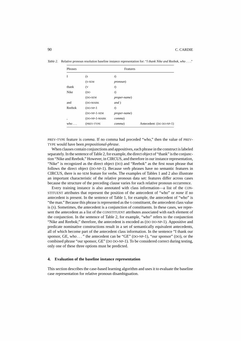
Table 2. Relative pronoun resolution baseline instance representation for: “I thank Nike and Reebok, who. . . .”

Phrases Features

I (S t)

(S-SEM pronoun)

thank (V t)

Nike (DO t)

(DO-SEM proper-name)

and (DO-MARK and)

Reebok (DO-NP-1 t)

(DO-NP-1-SEM proper-name)

, (DO-NP-1-MARK comma)

who . . . (PREV-TYPE comma) Antecedent: (DO DO-NP-1)

PREV-TYPE feature iscomma. If no comma had preceded “who,” then the value ofPREV-TYPE would have beenprepositional-phrase.

When clauses contain conjunctions and appositives, each phrase in the construct is labeledseparately. In the sentence of Table 2, for example, the direct object of “thank” is the conjunc-tion “Nike and Reebok.” However, in CIRCUS, and therefore in our instance representation,“Nike” is recognized as the direct object (DO) and “Reebok” as the first noun phrase thatfollows the direct object (DO-NP-1). Because verb phrases have no semantic features inCIRCUS, there is noSEM feature for verbs. The examples of Tables 1 and 2 also illustratean important characteristic of the relative pronoun data set: features differ across casesbecause the structure of the preceding clause varies for each relative pronoun occurrence.

Every training instance is also annotated with class information—a list of theCON-STITUENT attributes that represent the position of the antecedent of “who” ornoneif noantecedent is present. In the sentence of Table 1, for example, the antecedent of “who” is“the man.” Because this phrase is represented as theSconstituent, the antecedent class valueis (S). Sometimes, the antecedent is a conjunction of constituents. In these cases, we repre-sent the antecedent as a list of theCONSTITUENTattributes associated with each element ofthe conjunction. In the sentence of Table 2, for example, “who” refers to the conjunction“Nike and Reebok;” therefore, the antecedent is encoded as (DO DO-NP-1). Appositive andpredicate nominative constructions result in a set of semantically equivalent antecedents,all of which become part of the antecedent class information. In the sentence “I thank oursponsor, GE, who. . . ” the antecedent can be “GE” (DO-NP-1), “our sponsor” (DO), or thecombined phrase “our sponsor, GE” (DO DO-NP-1). To be considered correct during testing,only one of these three options must be predicted.

4. Evaluation of the baseline instance representation

This section describes the case-based learning algorithm and uses it to evaluate the baselinecase representation for relative pronoun disambiguation.


4.1. The case-based learning algorithm

Throughout the paper, we employ a simple case-based, or instance-based, learning algorithm(e.g., Aha, Kibler, & Albert, 1991). During the training phase, all relative pronoun instancesare simply stored in a case base. Then, given a new relative pronoun instance, a weighted1-nearest neighbor (1-nn) case retrieval algorithm predicts its antecedent:

1. Compare the test case,X, to each case,Y, in the case base and calculate for each pair:

|N|∑i=1

wNi ∗match(XNi ,YNi

)whereN denotes the test case features,wNi is the weight of thei th feature inN, XNi isthe value of featureNi in the test case,YNi is the value ofNi in the training case, andmatch(a, b) is a function that returns 1 ifa andb are equal and 0 otherwise. (For thebaseline experiments,wNi = 1.)

2. Return the cases with the highest score.3. If a single case is retrieved, use its antecedent class information to find the antecedent

in the test case. Otherwise, let the retrieved cases vote on the position of the antecedent.

If the antecedent of the top-ranked case isDO (direct object), for example, then the directobject of the test case sentence would be selected as the antecedent. Sometimes, however, theretrieved case may list more than one option as the antecedent (for appositive and predicatenominative constructions). In these cases, we choose the first option in the antecedent listwhose constituents overlap with those in the current example.

The above case retrieval algorithm matches only on features that appear in the test case.Alternatively, the retrieval algorithm could normalize the feature set across the trainingcases and then match with respect to this expanded feature set. We obtained comparableperformance on the relative pronoun task when using a normalized feature set, but will notdiscuss those results here.

4.2. The relative pronoun data set

The relative pronoun data set contains 241 instances—CIRCUS generates one case for eachoccurrence of “who” in 150 texts from the MUC-3 corpus. The correct antecedent for eachcase must be specified by a human supervisor or by accessing a version of the training corpusthat has been annotated with relative clause attachment information. For the experimentsin this paper, we made one pass through the data set to correct a small number of obviousparsing and semantic class disambiguation errors.

The performance of the learning algorithm depends, in part, on the underlying charac-teristics of this data set. First, instances contain between two and 31 features and representclauses that have from one to 11 phrases. 77% of the cases are unique. In addition, theantecedent class takes on 60 distinct values across the data set. In particular, there are ten

92 C. CARDIE

instances with unique antecedent values. This establishes an upper limit of 96% accuracywhen using the baseline instance representation.

The data set contains just one pair of ‘ambiguous’ instances that have the same set ofattribute-value pairs, but a different antecedent value. Here our instance representation wastoo coarse to differentiate wh-word contexts. In particular, it lacked the necessary lexicalfeatures to distinguish one type of pronoun from another. More importantly, 51% of thecases involve syntactically ambiguous constructs with respect to relative pronoun resolution.These include sentences like the following, where the head noun of either constituent1 orconstituent2 is a syntactically viable antecedent:

I walked [with the man]2 [from Detroit]1 who . . .I saw [the daughter]2 [of the colonel]1 who . . .

In theory, the case-based learning algorithm can use the available semantic class informa-tion or punctuation to correctly handle most of these cases (e.g. “Detroit” is an unlikelyantecedent ofwho since it is a location). Even so, a small number of cases (like the secondexample) will remain ambiguous without additional context.

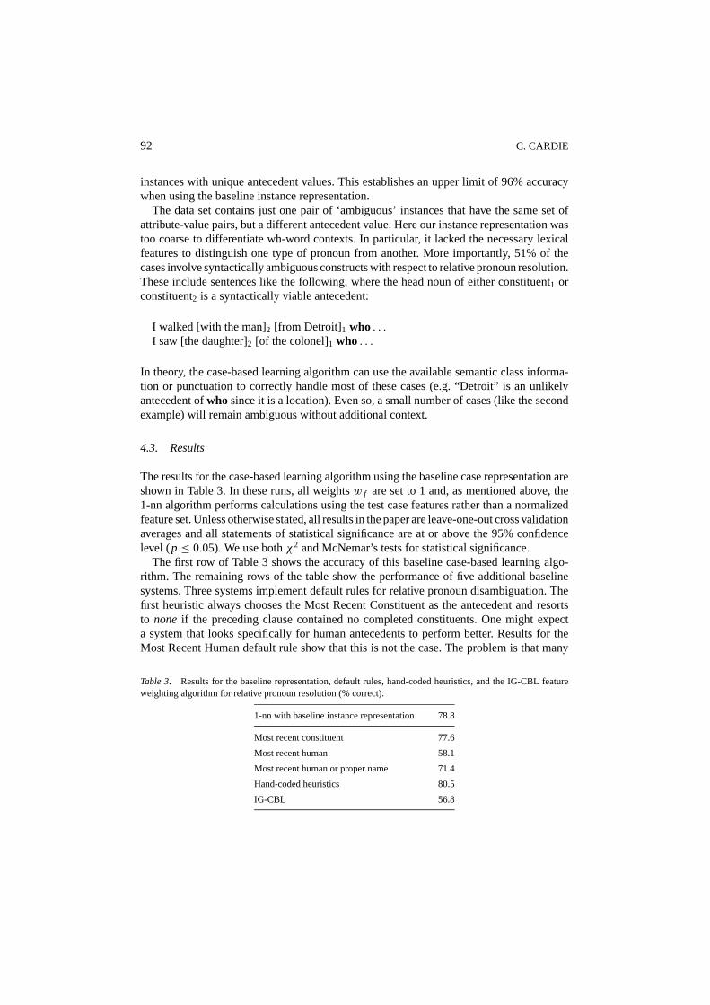
4.3. Results

The results for the case-based learning algorithm using the baseline case representation areshown in Table 3. In these runs, all weightsw f are set to 1 and, as mentioned above, the1-nn algorithm performs calculations using the test case features rather than a normalizedfeature set. Unless otherwise stated, all results in the paper are leave-one-out cross validationaverages and all statements of statistical significance are at or above the 95% confidencelevel (p ≤ 0.05). We use bothχ2 and McNemar’s tests for statistical significance.

The first row of Table 3 shows the accuracy of this baseline case-based learning algo-rithm. The remaining rows of the table show the performance of five additional baselinesystems. Three systems implement default rules for relative pronoun disambiguation. Thefirst heuristic always chooses the Most Recent Constituent as the antecedent and resortsto none if the preceding clause contained no completed constituents. One might expecta system that looks specifically for human antecedents to perform better. Results for theMost Recent Human default rule show that this is not the case. The problem is that many

Table 3. Results for the baseline representation, default rules, hand-coded heuristics, and the IG-CBL featureweighting algorithm for relative pronoun resolution (% correct).

1-nn with baseline instance representation 78.8

Most recent constituent 77.6

Most recent human 58.1

Most recent human or proper name 71.4

Hand-coded heuristics 80.5

IG-CBL 56.8


legitimate antecedents of “who” are characterized by semantic features other thanhuman.Unfortunately, looking for more complicated semantic feature combinations like those ofthe third rule (Most Recent Human or Proper Name) does no better than the simplest defaultrule.

The fourth baseline system of Table 3 employs a set of hand-crafted heuristics for relativepronoun resolution that were developed for use in the MUC-3 performance evaluation. Theheuristics consisted of approximately 30 rules. The following are examples:

If there is no verb and no subject in the preceding clause, and the last constituent was anNP, then the antecedent is the head of the last constituent.

If there is no verb in the preceding clause, and the token that precedes “who” is a comma,then the antecedent is the head of the subject of the preceding clause.

In general, the rules make use of the same syntactic and semantic information that is encodedin the baseline instance representation. They were originally based on approximately 50instances of relative pronouns taken from the MUC terrorism corpus, but were modifiedover a nine-month period to handle counter-examples as they were encountered duringtesting of the full information extraction system.

The results in Table 3 indicate that the baseline 1-nn system (78.8% correct) performsas well as the best default rule (77.6% correct) and below that of the hand-coded heuristics(80.5% correct). Bothχ2 and McNemar’s significance tests indicate, however, that all threesystems are indistinguishable from one another in terms of statistical significance. Althoughthe accuracies of the baseline representation and the Most Recent Constituent default rule arequite close, their behavior is qualitatively different. As expected, the baseline representationperforms markedly worse than the default rule for antecedents that immediately precederelative pronoun; however, it performs markedly better than the default rule for complexantecedents (conjunctions and appositives), for subject antecedents, and for detecting when“who” is not being used as a relative pronoun (antecedent= none). The final row in Table 3is explained in the next section.

4.4. Comparison to IG-CBL

This section compares the performance of the baseline case-based learning algorithm toIG-CBL (Cardie & Howe, 1997), a feature weighting algorithm that has shown good perfor-mance across a number of natural language learning tasks. IG-CBL is a weighted k-nearestneighbor algorithm that is a straightforward composition of two existing approaches forfeature selection and feature weighting. IG-CBL first uses a decision tree for feature se-lection as described in Cardie (1993) and briefly below. The goal in this step is to prunefeatures from the representation so that the case-based learning algorithm can ignore thementirely. IG-CBL then assigns each remaining feature a weight according to its informationgain across the training cases as done in the IB1-IG algorithm (Daelemans, van den Bosch,& Zavrel, 1999). The intent here is to weight each feature relative to its overall importancein the data set. There are three steps to the IG-CBL training phase:

94 C. CARDIE

1. Create the case base.For this, we simply store all of the training instances.2. Use the training instances to create a decision tree for the learning task.Our experiments

use C4.5 (Quinlan, 1993).3. Compute feature weights for use during case retrieval.For each feature,f , we compute

a weight,w f , as follows:

w f = G( f ) if f is in the tree of step 2;

w f = 0 otherwise;

whereG( f ) is the information gain ratio off as computed across all training instancesby C4.5.

To apply the IG-CBL algorithm to the relative pronoun data set, we first normalize theinstances with respect to the entire feature set, filling in anil value for missing features.After training, the class value for a novel instance is determined using a weighted k-nn caseretrieval algorithm identical to that of the baseline case-based learning algorithm exceptthat feature weights are computed as above.

We see from Table 3 that the IG-CBL feature-weighting approach works very poorly forthe relative pronoun task although it has worked well for other natural language learningproblems including part-of-speech tagging, semantic class tagging, prepositional phraseattachment, grapheme-to-phoneme conversion, and noun phrase chunking (Cardie, 1993;Daelemans et al., 1999). We believe that IG-CBL works poorly because of the large numberof antecedent classes and because the information gain bias is not appropriate for the relativepronoun task, especially with normalized instances that contain mostly missing values. Wewill see better performance of IG-CBL on the data sets of Section 7.

5. Incorporating the cognitive biases

In the following subsections, we modify the baseline representation in response to threecognitive biases and measure the effects of those changes on the learning algorithm’s abilityto predict relative pronoun antecedents.

5.1. Incorporating the subject accessibility bias

A number of studies in psycholinguistics have noted the special importance of the firstitem mentioned in a sentence (e.g., Gernsbacher, Hargreaves, & Beeman, 1989; Carreiras,Gernsbacher, & Villa, 1995). In particular, it has been shown that the accessibility of thefirst actor of a sentence remains high even at the end of a sentence (Gernsbacher et al.,1989). The effect of thissubject accessibility biason processing relative clauses was alsonoted in King and Just (1991) and is an example of a more generalfocus of attention bias.In computer vision learning problems, for example, the brightest object in view may bea highly accessible object for the learning agent; in aural tasks, very loud or high-pitchedsounds may be highly accessible. We propose to incorporate the subject accessibility biasinto the baseline case representation by increasing the weights for any features associatedwith the subject of the clause preceding the relative pronoun. Weights for the subject features


Table 4. The effect of the subject accessibility bias on relative pronoun resolution (% correct).

Baseline Subject wt= 2 Subject wt= 5 Subject wt= 8 Subject wt= 12

78.8 76.7 75.5 76.3 75.9

are increased as a function of a fixed increment, thesubject weight. More specifically, thesubject weight is divided evenly across all features associated with the subject (i.e.,S, S-SEM, and possiblyS-PUNCor S-MARK) and then added to the original weight for each subjectfeature.

Table 4 shows the effects on relative pronoun resolution when the subject weight is 2, 5,8, and 12: incorporation of the subject accessibility bias never improves relative pronoundisambiguation when compared to the baseline representation, although dips in performanceare never statistically significant using theχ2 test. McNemar’s test indicates significantdifferences between the baseline representation and the subject-weighted representationwhen the weight is 5 or 12. Higher subject weights were tested, but provide no improvementin performance.

At first these results may seem surprising, but the baseline representation produced byCIRCUS already somewhat encodes the subject accessibility bias by explicitly recognizingthe subject as a major constituent of the sentence (i.e.,S) rather than labeling it merely as alow-level noun phrase (i.e.,NP). (Removing this bias from the baseline representation causesa drop in performance from 78.8% to 75.5%.) It may be that the original encoding of thebias is adequate or that additional modifications to the baseline representation are requiredbefore the subject accessibility bias can have a positive effect. In addition, the subjectaccessibility bias affects a relatively small number of features. Some cases have no subjectfeatures because no subject was identified in the clause preceding the relative pronoun.For these cases, the subject accessibility bias plays no role at all. An analysis of errorsindicates that the baseline representation performs slightly better than the subject-weightedrepresentation (weight= 2) across all of the major antecedent types.

5.2. Incorporating the recency bias

In processing language, people consistently show a bias towards the use of the most recentinformation (e.g., Kimball, 1973; Nicol, 1988; Gibson, 1990; Gibson et al., 1993). In par-ticular, Frazier and Fodor (1978), Cuetos and Mitchell (1988), and others have investigatedthe importance of recency in finding the antecedents of relative pronouns. They found thatfor English there is a preference for choosing the most recent noun phrase as the antecedentin sentences where the antecedent of the relative pronoun is ambiguous. For example, insentences likeThe journalist interviewed the daughter of the colonel who had the accident,people assume that “who” refers to “the colonel” rather than “the daughter of the colonel.”

The feature selection algorithm translates this recency bias into representational changesfor the training and test instances in two ways. The first is a direct modification of thefeature set; the second modifies the weights to indicate a constituent’s distance from therelative pronoun. In the first approach, we rename the features according to the position of

96 C. CARDIE

Table 5. Incorporating the recency bias using a right-to-left labeling.

Baseline representation Sentence Right-to-left labeling

(S t) it (S t)

(S-SEM entity) (S-SEM entity)

(V t) was (V t)

(DO t) the hardliners (NP-2 t)

(DO-SEM human) (NP-2 human)

(DO-PP-1 t) in Congress (PP-1 t)

(DO-PP-1-PREPin) (PP-1-PREPin)

(DO-PP-1-SEM entity) (PP-1-SEM entity)

(PREV-TYPE prepositional-phrase) who . . . (PREV-TYPE prepositional-phrase)

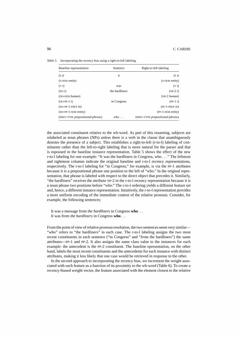
the associated constituent relative to the wh-word. As part of this renaming, subjects arerelabeled as noun phrases (NPs) unless there is a verb in the clause that unambiguouslydenotes the presence of a subject. This establishes a right-to-left (r-to-l) labeling of con-stituents rather than the left-to-right labeling that is more natural for the parser and thatis espoused in the baseline instance representation. Table 5 shows the effect of the newr-to-l labeling for one example: “It was the hardliners in Congress, who. . . ” The leftmostand rightmost columns indicate the original baseline and r-to-l recency representations,respectively. The r-to-l labeling for “in Congress,” for example, is via thePP-1 attributesbecause it is a prepositional phrase one position to the left of “who.” In the original repre-sentation, that phrase is labeled with respect to the direct object that precedes it. Similarly,“the hardliners” receives the attributeNP-2 in the r-to-l recency representation because it isa noun phrase two positions before “who.” The r-to-l ordering yields a different feature setand, hence, a different instance representation. Intuitively, the r-to-l representation providesa more uniform encoding of the immediate context of the relative pronoun. Consider, forexample, the following sentences:

It was a message fromthe hardlinersin Congresswho . . .It was fromthe hardlinersin Congresswho . . .

From the point of view of relative pronoun resolution, the two sentences seem very similar—“who” refers to “the hardliners” in each case. The r-to-l labeling assigns the two mostrecent constituents in each sentence (“in Congress” and “from the hardliners”) the sameattributes—PP-1 andPP-2. It also assigns the same class value to the instances for eachexample: the antecedent is thePP-2 constituent. The baseline epresentation, on the otherhand, labels the most recent constituents and the antecedents for each instance with distinctattributes, making it less likely that one case would be retrieved in response to the other.

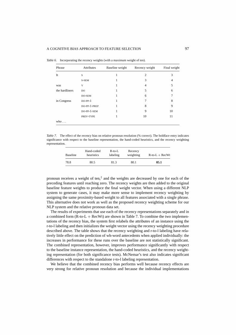
In the second approach to incorporating the recency bias, we increment the weight asso-ciated with each feature as a function of its proximity to the wh-word (Table 6). To create arecency-biased weight vector, the feature associated with the element closest to the relative


Table 6. Incorporating the recency weights (with a maximum weight of ten).

Phrase Attributes Baseline weight Recency weight Final weight

It S 1 2 3

S-SEM 1 3 4

was V 1 4 5

the hardliners DO 1 5 6

DO-SEM 1 6 7

in Congress DO-PP-1 1 7 8

DO-PP-1-PREP 1 8 9

DO-PP-1-SEM 1 9 10

PREV-TYPE 1 10 11

who . . .

Table 7. The effect of the recency bias on relative pronoun resolution (% correct). The boldface entry indicatessignificance with respect to the baseline representation, the hand-coded heuristics, and the recency weightingrepresentation.

Hand-coded R-to-L RecencyBaseline heuristics labeling weighting R-to-L+ RecWt

78.8 80.5 81.3 80.1 85.1

pronoun receives a weight of ten,2 and the weights are decreased by one for each of thepreceding features until reaching zero. The recency weights are then added to the originalbaseline feature weights to produce the final weight vector. When using a different NLPsystem to generate cases, it may make more sense to implement recency weighting byassigning the same proximity-based weight to all features associated with a single phrase.This alternative does not work as well as the proposed recency weighting scheme for ourNLP system and the relative pronoun data set.

The results of experiments that use each of the recency representations separately and ina combined form (R-to-L+ RecWt) are shown in Table 7. To combine the two implemen-tations of the recency bias, the system first relabels the attributes of an instance using ther-to-l labeling and then initializes the weight vector using the recency weighting proceduredescribed above. The table shows that the recency weighting and r-to-l labeling have rela-tively little effect on the prediction of wh-word antecedents when applied individually: theincreases in performance for these runs over the baseline are not statistically significant.The combined representation, however, improves performance significantly with respectto the baseline instance representation, the hand-coded heuristics, and the recency weight-ing representation (for both significance tests). McNemar’s test also indicates significantdifferences with respect to the standalone r-to-l labeling representation.

We believe that the combined recency bias performs well because recency effects arevery strong for relative pronoun resolution and because the individual implementations

98 C. CARDIE

of the recency bias complement one another. In particular, the representation of the localcontext of the wh-word provided by the r-to-l labeling is critical for finding antecedents. Therecency weighting representation lacks such a representation of local context, but providesan additional emphasis on those constituents closest to the relative pronoun.

One can get a sense of the broad changes to the instance space caused by the r-to-l recencylabeling by re-examining some of the original data set characteristics after applying thisbias. As described in Section 4.2, the data set encoded using the baseline case representationexhibits 60 distinct antecedents. After incorporating the r-to-l recency bias, this number isreduced to 39. In addition, the number of instances with unique antecedents is similarlyreduced—from ten to one. In spite of these reductions in data set complexity, the numberof instance types remains about the same: of the 241 cases, 184 (76%) are unique vs. 186(77%) using the baseline representation.

In an analysis of the results, we see that for 25 test cases, the combined recency bias iscorrect when the baseline representation is incorrect; the reverse is true only ten times. Ingeneral, the combined representation does markedly better than the baseline in recognizingwhen “who” is not being used as a relative pronoun. Although the combined represen-tation performs better than the baseline for antecedents at all distances from the relativepronoun, over half of the differences involve ‘middle distance’ antecedents that are two orthree phrases before the relative pronoun. Two instances that the combined recency rep-resentation gets correct when the baseline does not are listed here. (Subscripts denote theantecedent phrases selected using each representation. A subscript ofbothmeans that boththe baseline and combined recency representations selected the phrase as a component ofthe antecedent.)

Ordonez added: I was aware that Pena wanted to get rid of somebody, but Ibaselineneverlearnedwho they were going to kill until. . . (Correct antecedent is nonecombined recency).

Spaniard Jose Maria Martinezboth, Frenchman Roberto Lisandycombined recency, and Ital-ian Dino Rossycombined recency, who were staying. . .

5.3. Incorporating the restricted memory bias

Psychological studies have determined that people can remember at most seven plus or mi-nus two items at any one time (Miller, 1956). More recently, Daneman and Carpenter (1980;1983) show that working memory capacity affects a subject’s ability to find the referentsof pronouns over varying distances. Also, King and Just (1991) show that differences inworking memory capacity can cause differences in the reading time and comprehension ofcertain classes of relative clauses. Moreover, it has been hypothesized that language learn-ing in humans is successful precisely because limits on information processing capacitiesallow children to ignore much of the linguistic data they receive (Newport, 1990). Somecomputational language learning systems (e.g., Elman, 1990) actually build a short termmemory directly into the architecture of the system.

It should be clear that the baseline instance representation for the relative pronoun taskdoes not make use of short term memory limitations: the learning algorithm uses all availablefeatures during case retrieval. Short term memory studies, however, do not explicitly state


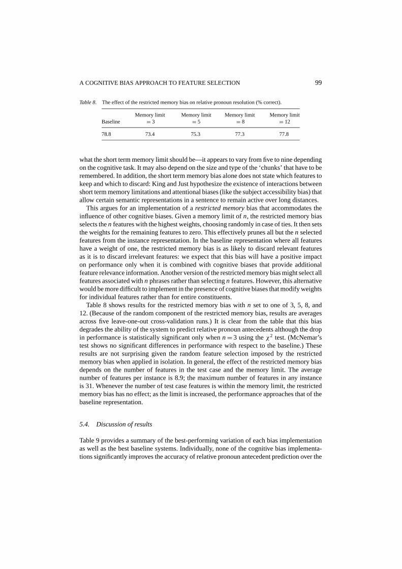
Table 8. The effect of the restricted memory bias on relative pronoun resolution (% correct).

Memory limit Memory limit Memory limit Memory limitBaseline = 3 = 5 = 8 = 12

78.8 73.4 75.3 77.3 77.8

what the short term memory limit should be—it appears to vary from five to nine dependingon the cognitive task. It may also depend on the size and type of the ‘chunks’ that have to beremembered. In addition, the short term memory bias alone does not state which features tokeep and which to discard: King and Just hypothesize the existence of interactions betweenshort term memory limitations and attentional biases (like the subject accessibility bias) thatallow certain semantic representations in a sentence to remain active over long distances.

This argues for an implementation of arestricted memorybias that accommodates theinfluence of other cognitive biases. Given a memory limit ofn, the restricted memory biasselects then features with the highest weights, choosing randomly in case of ties. It then setsthe weights for the remaining features to zero. This effectively prunes all but then selectedfeatures from the instance representation. In the baseline representation where all featureshave a weight of one, the restricted memory bias is as likely to discard relevant featuresas it is to discard irrelevant features: we expect that this bias will have a positive impacton performance only when it is combined with cognitive biases that provide additionalfeature relevance information. Another version of the restricted memory bias might select allfeatures associated withn phrases rather than selectingn features. However, this alternativewould be more difficult to implement in the presence of cognitive biases that modify weightsfor individual features rather than for entire constituents.

Table 8 shows results for the restricted memory bias withn set to one of 3, 5, 8, and12. (Because of the random component of the restricted memory bias, results are averagesacross five leave-one-out cross-validation runs.) It is clear from the table that this biasdegrades the ability of the system to predict relative pronoun antecedents although the dropin performance is statistically significant only whenn= 3 using theχ2 test. (McNemar’stest shows no significant differences in performance with respect to the baseline.) Theseresults are not surprising given the random feature selection imposed by the restrictedmemory bias when applied in isolation. In general, the effect of the restricted memory biasdepends on the number of features in the test case and the memory limit. The averagenumber of features per instance is 8.9; the maximum number of features in any instanceis 31. Whenever the number of test case features is within the memory limit, the restrictedmemory bias has no effect; as the limit is increased, the performance approaches that of thebaseline representation.

5.4. Discussion of results

Table 9 provides a summary of the best-performing variation of each bias implementationas well as the best baseline systems. Individually, none of the cognitive bias implementa-tions significantly improves the accuracy of relative pronoun antecedent prediction over the

100 C. CARDIE

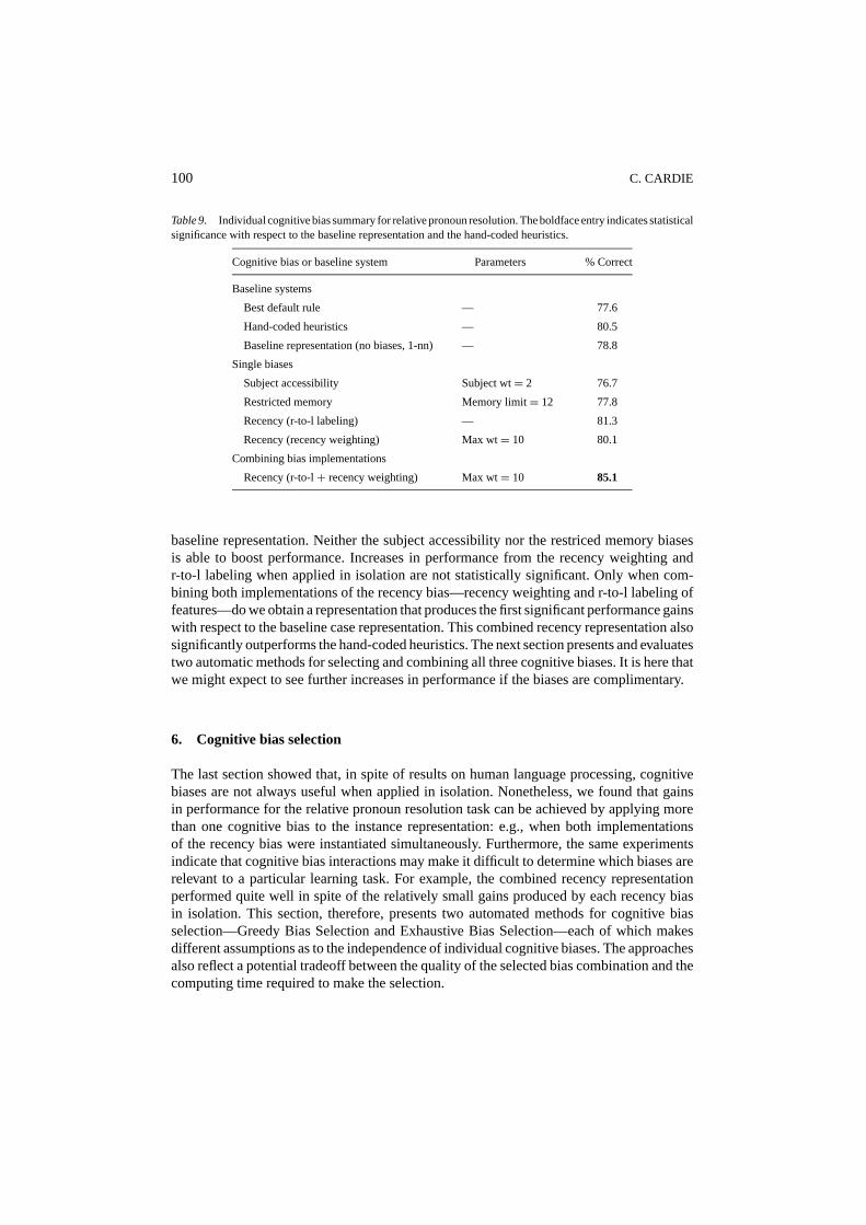
Table 9. Individual cognitive bias summary for relative pronoun resolution. The boldface entry indicates statisticalsignificance with respect to the baseline representation and the hand-coded heuristics.

Cognitive bias or baseline system Parameters % Correct

Baseline systems

Best default rule — 77.6

Hand-coded heuristics — 80.5

Baseline representation (no biases, 1-nn) — 78.8

Single biases

Subject accessibility Subject wt= 2 76.7

Restricted memory Memory limit= 12 77.8

Recency (r-to-l labeling) — 81.3

Recency (recency weighting) Max wt= 10 80.1

Combining bias implementations

Recency (r-to-l+ recency weighting) Max wt= 10 85.1

baseline representation. Neither the subject accessibility nor the restriced memory biasesis able to boost performance. Increases in performance from the recency weighting andr-to-l labeling when applied in isolation are not statistically significant. Only when com-bining both implementations of the recency bias—recency weighting and r-to-l labeling offeatures—do we obtain a representation that produces the first significant performance gainswith respect to the baseline case representation. This combined recency representation alsosignificantly outperforms the hand-coded heuristics. The next section presents and evaluatestwo automatic methods for selecting and combining all three cognitive biases. It is here thatwe might expect to see further increases in performance if the biases are complimentary.

6. Cognitive bias selection

The last section showed that, in spite of results on human language processing, cognitivebiases are not always useful when applied in isolation. Nonetheless, we found that gainsin performance for the relative pronoun resolution task can be achieved by applying morethan one cognitive bias to the instance representation: e.g., when both implementationsof the recency bias were instantiated simultaneously. Furthermore, the same experimentsindicate that cognitive bias interactions may make it difficult to determine which biases arerelevant to a particular learning task. For example, the combined recency representationperformed quite well in spite of the relatively small gains produced by each recency biasin isolation. This section, therefore, presents two automated methods for cognitive biasselection—Greedy Bias Selection and Exhaustive Bias Selection—each of which makesdifferent assumptions as to the independence of individual cognitive biases. The approachesalso reflect a potential tradeoff between the quality of the selected bias combination and thecomputing time required to make the selection.


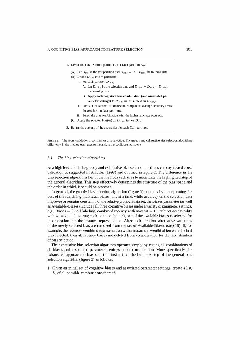
1. Divide the dataD into n partitions. For each partitionDtest,

(A) Let Dtest be the test partition andDtrain = D − Dtest, the training data.

(B) Divide Dtrain into m partitions.

i. For each partitionDtrains

A. Let Dtrains be the selection data andDtrainl = Dtrain − Dtrains ,

the learning data.

B. Apply each cognitive bias combination (and associated pa-

rameter settings) toDtrainl in turn. Test on Dtrains .

ii. For each bias combination tested, compute its average accuracy across

them selection data partitions.

iii. Select the bias combination with the highest average accuracy.

(C) Apply the selected bias(es) onDtrain; test onDtest.

2. Return the average of the accuracies for eachDtest partition.

Figure 2. The cross-validation algorithm for bias selection. The greedy and exhaustive bias selection algorithmsdiffer only in the method each uses to instantiate the boldface step above.

6.1. The bias selection algorithms

At a high level, both the greedy and exhaustive bias selection methods employ nested crossvalidation as suggested in Schaffer (1993) and outlined in figure 2. The difference in thebias selection algorithms lies in the methods each uses to instantiate the highlighted step ofthe general algorithm. This step effectively determines the structure of the bias space andthe order in which it should be searched.

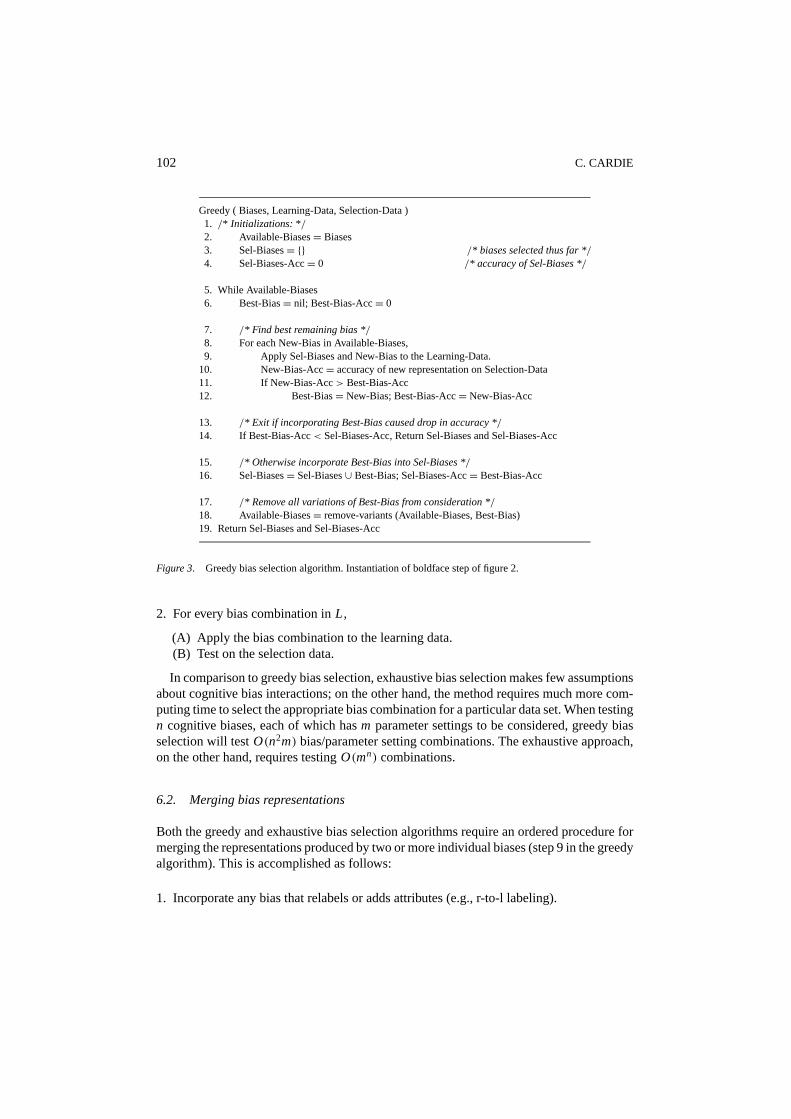
In general, the greedy bias selection algorithm (figure 3) operates by incorporating thebest of the remaining individual biases, one at a time, while accuracy on the selection dataimproves or remains constant. For the relative pronoun data set, the Biases parameter (as wellas Available-Biases) includes all three cognitive biases under a variety of parameter settings,e.g., Biases= {r-to-l labeling, combined recency with max wt= 10, subject accessibilitywith wt = 2, . . . }. During each iteration (step 5), one of the available biases is selected forincorporation into the instance representation. After each iteration, alternative variationsof the newly selected bias are removed from the set of Available-Biases (step 18). If, forexample, the recency-weighting representation with a maximum weight of ten were the firstbias selected, then all recency biases are deleted from consideration for the next iterationof bias selection.

The exhaustive bias selection algorithm operates simply by testing all combinations ofall biases and associated parameter settings under consideration. More specifically, theexhaustive approach to bias selection instantiates the boldface step of the general biasselection algorithm (figure 2) as follows:

1. Given an initial set of cognitive biases and associated parameter settings, create a list,L, of all possible combinations thereof.

102 C. CARDIE

Greedy ( Biases, Learning-Data, Selection-Data )1. /* Initializations: */2. Available-Biases= Biases3. Sel-Biases= {} /* biases selected thus far */4. Sel-Biases-Acc= 0 /* accuracy of Sel-Biases */

5. While Available-Biases6. Best-Bias= nil; Best-Bias-Acc= 0

7. /* Find best remaining bias */8. For each New-Bias in Available-Biases,9. Apply Sel-Biases and New-Bias to the Learning-Data.

10. New-Bias-Acc= accuracy of new representation on Selection-Data11. If New-Bias-Acc> Best-Bias-Acc12. Best-Bias= New-Bias; Best-Bias-Acc= New-Bias-Acc

13. /* Exit if incorporating Best-Bias caused drop in accuracy */

14. If Best-Bias-Acc< Sel-Biases-Acc, Return Sel-Biases and Sel-Biases-Acc

15. /* Otherwise incorporate Best-Bias into Sel-Biases */

16. Sel-Biases= Sel-Biases∪ Best-Bias; Sel-Biases-Acc= Best-Bias-Acc

17. /* Remove all variations of Best-Bias from consideration */

18. Available-Biases= remove-variants (Available-Biases, Best-Bias)19. Return Sel-Biases and Sel-Biases-Acc

Figure 3. Greedy bias selection algorithm. Instantiation of boldface step of figure 2.

2. For every bias combination inL,

(A) Apply the bias combination to the learning data.(B) Test on the selection data.

In comparison to greedy bias selection, exhaustive bias selection makes few assumptionsabout cognitive bias interactions; on the other hand, the method requires much more com-puting time to select the appropriate bias combination for a particular data set. When testingn cognitive biases, each of which hasm parameter settings to be considered, greedy biasselection will testO(n2m) bias/parameter setting combinations. The exhaustive approach,on the other hand, requires testingO(mn) combinations.

6.2. Merging bias representations

Both the greedy and exhaustive bias selection algorithms require an ordered procedure formerging the representations produced by two or more individual biases (step 9 in the greedyalgorithm). This is accomplished as follows:

1. Incorporate any bias that relabels or adds attributes (e.g., r-to-l labeling).


2. Incorporate biases that modify feature weights by adding the weight vectors proposedby each bias (e.g., recency weighting, subject accessibility).

3. Incorporate biases that discard features (e.g., restricted memory bias).

As was the case with representations that included one cognitive bias, the combined biasrepresentations are created automatically. The user specifies only the list of biases to beapplied to the problem and any associated parameters.

6.3. Results

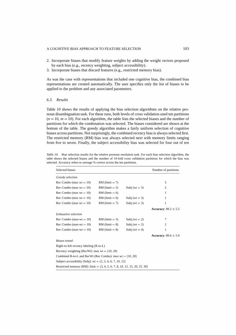
Table 10 shows the results of applying the bias selection algorithms on the relative pro-noun disambiguation task. For these runs, both levels of cross validation used ten partitions(n= 10,m= 10). For each algorithm, the table lists the selected biases and the number ofpartitions for which the combination was selected. The biases considered are shown at thebottom of the table. The greedy algorithm makes a fairly uniform selection of cognitivebiases across partitions. Not surprisingly, the combined recency bias is always selected first.The restricted memory (RM) bias was always selected next with memory limits rangingfrom five to seven. Finally, the subject accessibility bias was selected for four out of ten

Table 10. Bias selection results for the relative pronoun resolution task. For each bias selection algorithm, thetable shows the selected biases and the number of 10-fold cross validation partitions for which the bias wasselected. Accuracy refers to average % correct across the ten partitions.

Selected biases Number of partitions

Greedy selection

Rec Combo (max wt= 10) RM (limit = 7) 5

Rec Combo (max wt= 10) RM (limit = 5) Subj (wt= 3) 2

Rec Combo (max wt= 10) RM (limit = 6) 1



Accuracy: 89.2± 5.5

Exhaustive selection

Rec Combo (max-wt= 10) RM (limit = 5) Subj (wt= 2) 7



Accuracy: 89.6± 5.9

Biases tested:

Right-to-left recency labeling (R-to-L)

Recency weighting (RecWt): max wt= {10, 20}Combined R-to-L and RecWt (Rec Combo): max wt= {10, 20}Subject accessibility (Subj): wt= {2, 3, 4, 6, 7, 10, 12}Restricted memory (RM): limit= {3, 4, 5, 6, 7, 8, 10, 12, 15, 20, 25, 30}

104 C. CARDIE

partitions with a subject weight of three in all cases. The average accuracy of the repre-sentations created using greedy bias selection is 89.2%, which significantly outperformsthe baseline case representation, the best default rule, the hand-coded heuristics, and allof the individual cognitive biases. It also significantly outperforms the combined recencybiases.3

Exhaustive bias selection also chooses a fairly stable set of cognitive biases across par-titions: it selects the combined recency representation with a maximum weight of ten;the restricted memory bias with a relatively small memory limit (usually five); and thesubject accessibility bias with a small subject weight (usually two). The average accu-racy of the representations created using exhaustive bias selection is 89.6%. Like greedybias selection, exhaustive bias selection performs significantly better than the baseline caserepresentation, the best default rule, all of the individual biases, the hand-coded heuris-tics, and the combined recency biases. Significance tests indicate no difference in per-formance when compared to the greedy selection algorithm. The running time for one(outer-level) partition of exhaustive bias selection withn= 10 andm= 10 is about 17 min-utes on an Ultra Sparc 5. In contrast, one partition of greedy bias selection takes about twominutes.

6.4. Discussion and summary of results

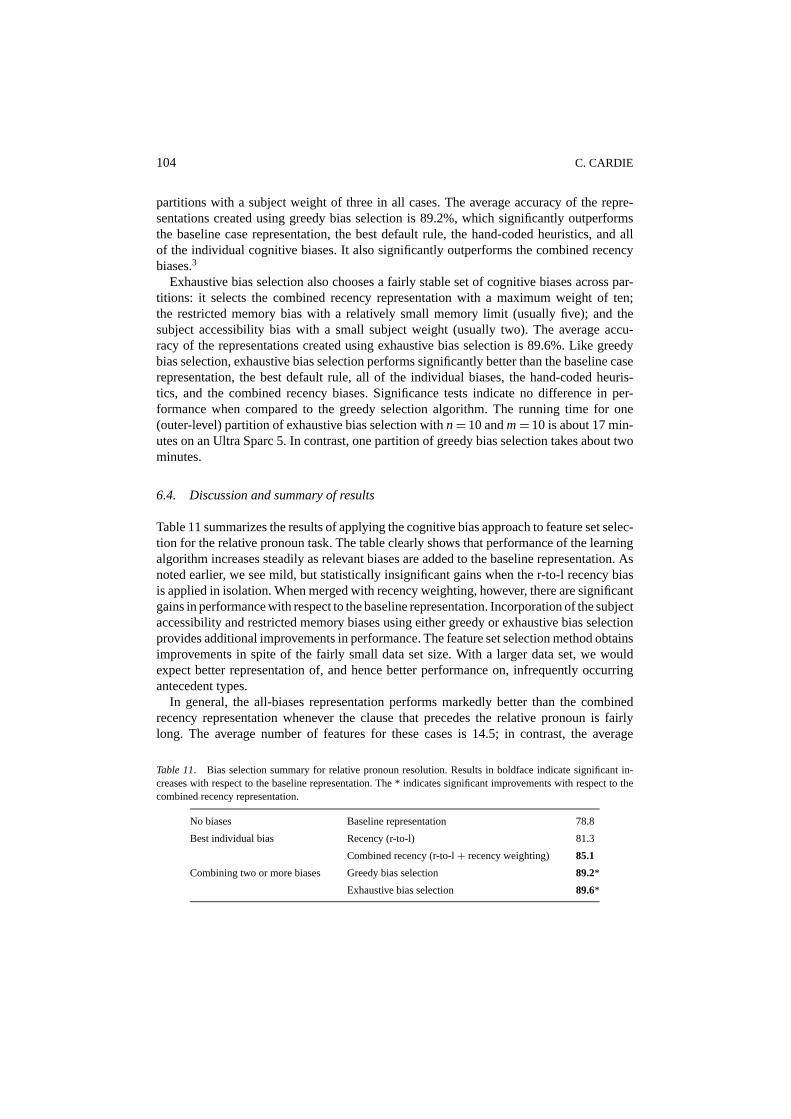
Table 11 summarizes the results of applying the cognitive bias approach to feature set selec-tion for the relative pronoun task. The table clearly shows that performance of the learningalgorithm increases steadily as relevant biases are added to the baseline representation. Asnoted earlier, we see mild, but statistically insignificant gains when the r-to-l recency biasis applied in isolation. When merged with recency weighting, however, there are significantgains in performance with respect to the baseline representation. Incorporation of the subjectaccessibility and restricted memory biases using either greedy or exhaustive bias selectionprovides additional improvements in performance. The feature set selection method obtainsimprovements in spite of the fairly small data set size. With a larger data set, we wouldexpect better representation of, and hence better performance on, infrequently occurringantecedent types.

In general, the all-biases representation performs markedly better than the combinedrecency representation whenever the clause that precedes the relative pronoun is fairlylong. The average number of features for these cases is 14.5; in contrast, the average

Table 11. Bias selection summary for relative pronoun resolution. Results in boldface indicate significant in-creases with respect to the baseline representation. The * indicates significant improvements with respect to thecombined recency representation.

No biases Baseline representation 78.8

Best individual bias Recency (r-to-l) 81.3

Combined recency (r-to-l+ recency weighting) 85.1

Combining two or more biases Greedy bias selection 89.2*

Exhaustive bias selection 89.6*


number features per case for the entire data set is 8.9. It is likely that the restricted memorybias is responsible for most of this improvement: it tends to prune features for distantconstituents in the all-biases representation, allowing the case-based learning algorithm toconcentrate on recent phrases during case retrieval. Furthermore, 73% of the improvementbetween the combined recency and all-biases representations is due to better performance onsyntactically ambiguous relative pronoun constructs (see Section 4.2). Two such examplesfollow:

The government publicly shows the horrorrecencyof womenall−biaseswho have been rapedin the prisons. . .

They also recommend that the persons who are going to carry out the abductionsshould select the victims from among politicians and membersall−biasesof the Colom-bian bourgeoisierecencywho have never distinguished themselves. . .

The two example shows that these syntactically ambiguous cases can be semantically diffi-cult as well: it is often hard for a person to provide consistent antecedent information in thepresence of collective or mass nouns (e.g., group, members). In addition, it is sometimesnecessary to read the relative clause in order to disambiguate the relative pronoun. Ourcurrent case representation, however, includes no features for phrases in the relative clauseitself, making it difficult to handle this type of ambiguity.

This section also showed that both the greedy and exhaustive search in conjunction withcross validation can be used for automatic bias selection. In particular, the experimentsindicate that greedy bias selection may be adequate whenever interactions among cognitivebiases are sufficiently limited. Finally, while exhaustive bias selection performs slightlybetter, the small gains in performance over greedy selection may not be worth the increasein running time.

7. Additional data sets

Thus far, we have concentrated on evaluating the cognitive bias approach to feature setselection using a single data set and three cognitive biases. In this section, we show thatthe approach is effective for tasks other than relative pronoun resolution. In particular, weapply the approach to three additional language learning tasks and make two more cognitivebiases available to the learning algorithm.

7.1. Handling unknown words

The additional data sets correspond to three lexical tagging tasks that address the problemsencountered by a natural language processing system when it reaches unknown words, i.e.,words not in the system lexicon. Given the context in which each unknown word occurs,our NLP system must predict the word’s part of speech as well as its general and specificsemantic class. Assume, for example, that the word “general” was an unknown word andthat the NLP system encountered the following two sentences from the MUC-3 information

106 C. CARDIE

extraction corpus:

Thegeneralconcern was that children might be killed.The terrorists killedGeneralBustillo.

In the first sentence, the system should indicate that the part of speech of “general” is anadjective; in the second sentence, it is a noun modifier. Similarly, given a two-level semanticfeature hierarchy, the system should determine that “general” is being used in its “universalentity” sense in the first case, but as a “person:military officer” in the second.

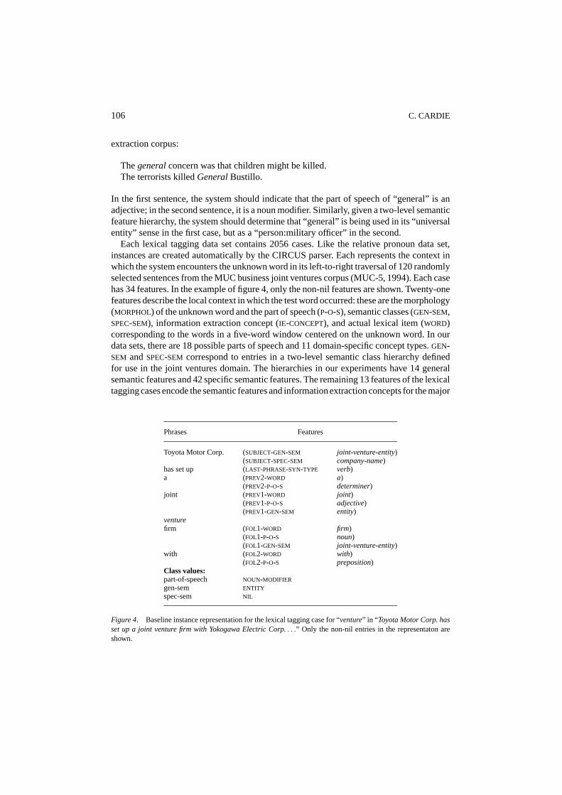
Each lexical tagging data set contains 2056 cases. Like the relative pronoun data set,instances are created automatically by the CIRCUS parser. Each represents the context inwhich the system encounters the unknown word in its left-to-right traversal of 120 randomlyselected sentences from the MUC business joint ventures corpus (MUC-5, 1994). Each casehas 34 features. In the example of figure 4, only the non-nil features are shown. Twenty-onefeatures describe the local context in which the test word occurred: these are the morphology(MORPHOL) of the unknown word and the part of speech (P-O-S), semantic classes (GEN-SEM,SPEC-SEM), information extraction concept (IE-CONCEPT), and actual lexical item (WORD)corresponding to the words in a five-word window centered on the unknown word. In ourdata sets, there are 18 possible parts of speech and 11 domain-specific concept types.GEN-SEM andSPEC-SEM correspond to entries in a two-level semantic class hierarchy definedfor use in the joint ventures domain. The hierarchies in our experiments have 14 generalsemantic features and 42 specific semantic features. The remaining 13 features of the lexicaltagging cases encode the semantic features and information extraction concepts for the major

Phrases Features

Toyota Motor Corp. (SUBJECT-GEN-SEM joint-venture-entity)(SUBJECT-SPEC-SEM company-name)

has set up (LAST-PHRASE-SYN-TYPE verb)a (PREV2-WORD a)

(PREV2-P-O-S determiner)joint (PREV1-WORD joint)

(PREV1-P-O-S adjective)(PREV1-GEN-SEM entity)

venturefirm (FOL1-WORD firm)

(FOL1-P-O-S noun)(FOL1-GEN-SEM joint-venture-entity)

with (FOL2-WORD with)(FOL2-P-O-S preposition)

Class values:part-of-speech NOUN-MODIFIER

gen-sem ENTITY

spec-sem NIL

Figure 4. Baseline instance representation for the lexical tagging case for “venture” in “ Toyota Motor Corp. hasset up a joint venture firm with Yokogawa Electric Corp.. . .” Only the non-nil entries in the representaton areshown.


syntactic constituents (i.e., the subject, verb, direct object, and most recent phrase) thathave been recognized at the time that the unknown word is encountered. Finally, each caseincludes the three class values to be predicted—the unknown word’s part-of-speech, andgeneral and specific semantic features. As was the case for relative pronoun resolution, thecase representation reflects the syntactic and semantic information available to CIRCUS asit processes a text. In this specification for handling unknown words, we treat each predictiontask independently.

In general, the features for the lexical tagging tasks are very similar to those used forrelative pronoun resolution. There are two main differences. First, we have encoded a richerdescription for the individual lexical items in close proximity to the unknown word. For therelative pronoun task, we concentrated on constituent-level representations. This differenceis reasonable since the current task is a lexical task rather than a structural attachmentdecision. However, since two-thirds of the features in the lexical tagging data sets nowrepresent neighboring tokens, the recency bias may have little effect. Second, we havealready discarded many irrelevant features from the representation. For example, the NLPsystem could easily have included features for every low-level phrase it recognizes (as wedid for relative pronoun resolution) and then relied on the learning algorithm to discardall irrelevant features. This preprocessing step inflates the performance of the baselinerepresentation. In addition, there may be less of a need for biases that discard features, likethe restricted memory bias. The data sets, therefore, may respond less readily to a numberof the cognitive biases. This will be a good test for the bias selection algorithms, which mayhave to recognize that not all available biases are relevant to the problems at hand.

7.2. The semantic priming and syntactic biases

To show that our approach can support a variety of cognitive biases, we define two additionalbiases for use with the lexical tagging tasks. The first issemantic priming. Semantic primingis a well-known cognitive effect—during on-line information processing, people tend torespond more quickly to words that are semantically related to entities currently involvedin the interpretation process. Our system implements semantic priming by increasing theweights for all semantic features in the baseline representation (e.g., the general or specificsemantic classes of words or constituents) by some specified value. This is only a verycoarse implementation of this bias, however. It encourages the case retrieval algorithm tomatch on semantic features, but ignores the problem of determining which entities are mostpertinent at the current point in processing. For this, we will rely on the other cognitivebiases. Analogously, we define asyntactic primingbias, which increases the weights forall features associated primarily with syntactic issues (e.g., the part of speech of words orsyntactic category of constituents) by some specified value.

7.3. Results on the lexical tagging tasks

In the experiments below, we investigate the use of all five biases—recency weighting,subject accessibility, restricted memory, semantic priming, and syntactic priming—on the

108 C. CARDIE

lexical tagging tasks. The right-to-left labeling bias is not applicable to these data sets, sinceall features are already effectively labeled with respect to the unknown word. To apply therecency weighting bias, we assume that features associated with the words in the five-wordwindow are more recent than any constituent features. Furthermore, we assume the follow-ing recency ‘ranking’ among terms in the five-word window: (1) unknown word features(MORPHOL); (2) features for the token immediately preceding the unknown word (PREV1);(3) features for the token immediately following the unknown word (FOL1); (4) features forthe second token that precedes the unknown word (PREV2); and (5) features for the secondtoken that follows the unknown word (FOL2). Allowing “following” tokens to incur weightsfrom the recency bias reflects the fact that lexical decision tasks often have an associatedtime delay of about 200 ms (Swinney, 1979), during which time subsequent tokens canbegin to be processed. All experiments employ 10-fold cross validation.4

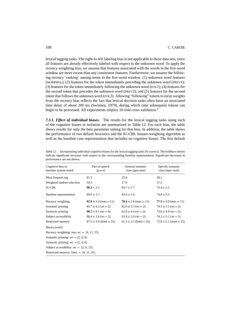
7.3.1. Effect of individual biases. The results for the lexical tagging tasks using eachof the cognitive biases in isolation are summarized in Table 12. For each bias, the tableshows results for only the best parameter setting for that bias. In addition, the table showsthe performance of two default heuristics and the IG-CBL feature-weighting algorithm aswell as the baseline case representation that includes no cognitive biases. The first default

Table 12. Incorporating individual cognitive biases for the lexical tagging tasks (% correct). The boldface entriesindicate significant increases with respect to the corresponding baseline representation. Significant decreases inperformance are not shown.

Cognitive bias or Part of speech General semantic Specific semanticbaseline system tested (p-o-s) class (gen-sem) class (spec-sem)

Most frequent tag 81.5 25.6 58.1

Weighted random selection 34.3 17.0 37.3

IG-CBL 90.3± 3.3 64.7± 5.7 73.4± 3.2

Baseline representation 89.0± 3.7 63.9± 5.4 74.8± 5.3

Recency weighting 92.9± 3.4 (max= 11) 70.4± 3.8 (max= 11) 77.5± 4.0 (max= 11)

Semantic priming 85.7± 4.2 (wt= 2) 62.0± 5.3 (wt= 2) 74.5± 5.1 (wt= 2)

Syntactic priming 90.7± 4.1 (wt= 6) 61.8± 4.4 (wt= 2) 73.0± 4.9 (wt= 2)

Subject accessibility 88.4± 3.6 (wt= 2) 63.9± 5.0 (wt= 2) 74.2± 5.1 (wt= 2)

Restricted memory 87.5± 3.0 (limit= 25) 61.5± 5.5 (limit= 25) 72.8± 5.1 (limit= 25)

Biases tested:

Recency weighting: max wt= {6, 11, 25}Semantic priming: wt={2, 4, 6}Syntactic priming: wt={2, 4, 6}Subject accessibility: wt= {2, 6, 12}Restricted memory: limit= {6, 11, 25}


heuristic selects the most frequently occurring class value; the second heuristic performs aweighted random selection based on class frequency. We see first that, unlike the relativepronoun data set, the baseline representation performs significantly better than the defaultheuristics. The IG-CBL feature-weighting approach also works well although it significantlyoutperforms the baseline representation only for part-of-speech tagging.

Like relative pronoun resolution, however, the recency bias provides significant increasesin performance over the baseline system. This is the case for all three data sets and in spiteof the fact that the baseline representation already focuses somewhat on recent items. Theonly other cognitive bias that boosts performance is the syntactic bias, which helps part-of-speech prediction. All other biases either significantly decrease performance on all datasets or have no effect on the lexical tagging task.

In general, the individual bias results for the lexical tagging tasks are not all that surprising.From a linguistic point of view, the recency weighting corresponds to giving preferentialstatus to features of those lexical items that are closest to the unknown word. This isconsistent with many successful lexical tagging approaches that classify tokens based onlyon information associated with one or two of the immediately preceding tokens.

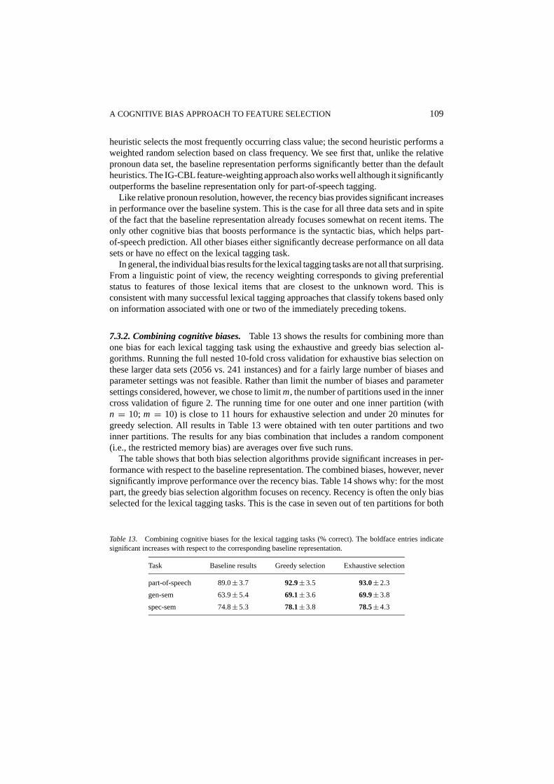
7.3.2. Combining cognitive biases.Table 13 shows the results for combining more thanone bias for each lexical tagging task using the exhaustive and greedy bias selection al-gorithms. Running the full nested 10-fold cross validation for exhaustive bias selection onthese larger data sets (2056 vs. 241 instances) and for a fairly large number of biases andparameter settings was not feasible. Rather than limit the number of biases and parametersettings considered, however, we chose to limitm, the number of partitions used in the innercross validation of figure 2. The running time for one outer and one inner partition (withn = 10; m = 10) is close to 11 hours for exhaustive selection and under 20 minutes forgreedy selection. All results in Table 13 were obtained with ten outer partitions and twoinner partitions. The results for any bias combination that includes a random component(i.e., the restricted memory bias) are averages over five such runs.

The table shows that both bias selection algorithms provide significant increases in per-formance with respect to the baseline representation. The combined biases, however, neversignificantly improve performance over the recency bias. Table 14 shows why: for the mostpart, the greedy bias selection algorithm focuses on recency. Recency is often the only biasselected for the lexical tagging tasks. This is the case in seven out of ten partitions for both

Table 13. Combining cognitive biases for the lexical tagging tasks (% correct). The boldface entries indicatesignificant increases with respect to the corresponding baseline representation.

Task Baseline results Greedy selection Exhaustive selection

part-of-speech 89.0± 3.7 92.9± 3.5 93.0± 2.3

gen-sem 63.9± 5.4 69.1± 3.6 69.9± 3.8

spec-sem 74.8± 5.3 78.1± 3.8 78.5± 4.3

110 C. CARDIE

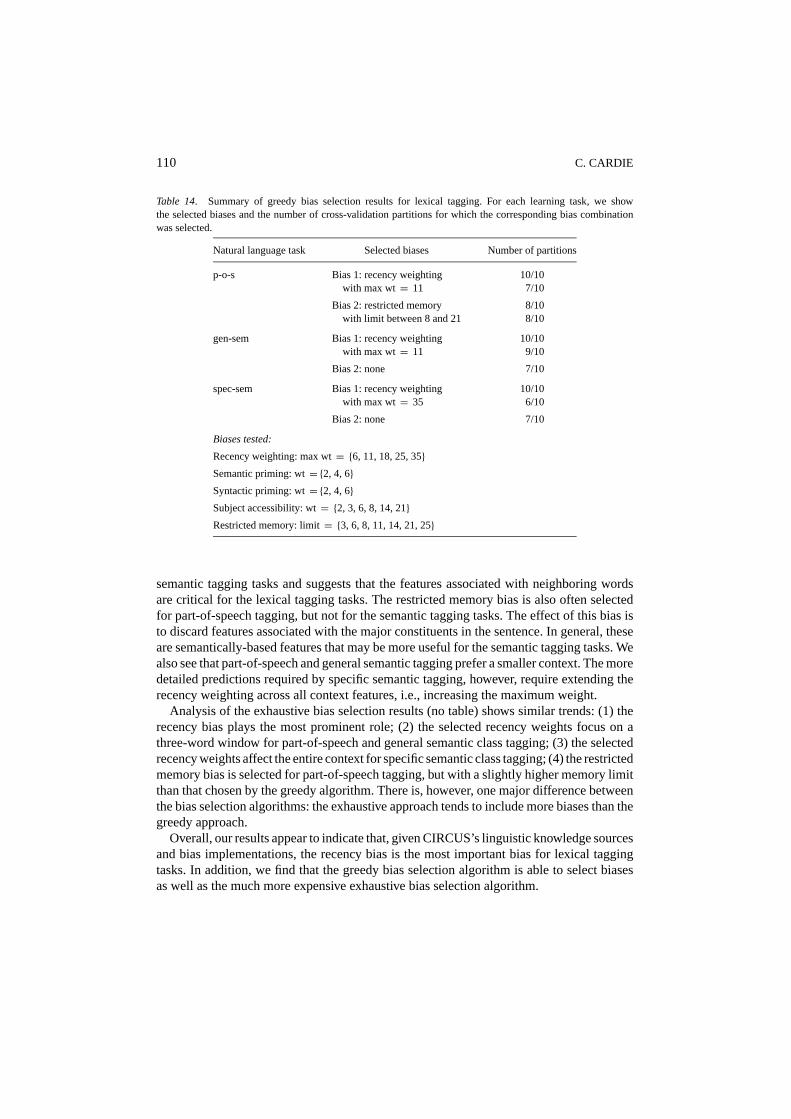
Table 14. Summary of greedy bias selection results for lexical tagging. For each learning task, we showthe selected biases and the number of cross-validation partitions for which the corresponding bias combinationwas selected.

Natural language task Selected biases Number of partitions

p-o-s Bias 1: recency weighting 10/10with max wt = 11 7/10

Bias 2: restricted memory 8/10with limit between 8 and 21 8/10

gen-sem Bias 1: recency weighting 10/10with max wt = 11 9/10

Bias 2: none 7/10

spec-sem Bias 1: recency weighting 10/10with max wt = 35 6/10

Bias 2: none 7/10

Biases tested:

Recency weighting: max wt= {6, 11, 18, 25, 35}Semantic priming: wt={2, 4, 6}Syntactic priming: wt={2, 4, 6}Subject accessibility: wt= {2, 3, 6, 8, 14, 21}Restricted memory: limit= {3, 6, 8, 11, 14, 21, 25}

semantic tagging tasks and suggests that the features associated with neighboring wordsare critical for the lexical tagging tasks. The restricted memory bias is also often selectedfor part-of-speech tagging, but not for the semantic tagging tasks. The effect of this bias isto discard features associated with the major constituents in the sentence. In general, theseare semantically-based features that may be more useful for the semantic tagging tasks. Wealso see that part-of-speech and general semantic tagging prefer a smaller context. The moredetailed predictions required by specific semantic tagging, however, require extending therecency weighting across all context features, i.e., increasing the maximum weight.

Analysis of the exhaustive bias selection results (no table) shows similar trends: (1) therecency bias plays the most prominent role; (2) the selected recency weights focus on athree-word window for part-of-speech and general semantic class tagging; (3) the selectedrecency weights affect the entire context for specific semantic class tagging; (4) the restrictedmemory bias is selected for part-of-speech tagging, but with a slightly higher memory limitthan that chosen by the greedy algorithm. There is, however, one major difference betweenthe bias selection algorithms: the exhaustive approach tends to include more biases than thegreedy approach.

Overall, our results appear to indicate that, given CIRCUS’s linguistic knowledge sourcesand bias implementations, the recency bias is the most important bias for lexical taggingtasks. In addition, we find that the greedy bias selection algorithm is able to select biasesas well as the much more expensive exhaustive bias selection algorithm.


8. Related work

Much previous work has addressed the role of biases in machine learning algorithms. Inparticular, there has been recent interest in automating methods for evaluating and selectingsuch biases. In their overview article to a special issue of this journal on the topic, Gordonand desJardins (1995) view bias selection as searching a space of learning biases. Withintheir framework, the work proposed here uses cognitive processing limitations as a typeof prior knowledge that guides the selection of an appropriaterepresentational biasforthe learning algorithm—the cognitive biases specify the set of primitive terms, or features,that define the space of allowable inductive hypotheses. Furthermore, our approach tobias selection uses greedy and exhaustive search in conjunction with cross validation asproceduralmeta-biases that order search in the representational bias space. In related work,Provost and Buchanan (1995) specify three techniques for buildinginductive policies, i.e.,policies for building strategies for bias selection. Our cognitive bias approach to featureset selection makes use of all three techniques: (1) cognitive biases add structure to thebias space, e.g., the restricted memory bias limits the number of features considered bythe learning algorithm; (2) the cognitive bias approach guides bias-space search, e.g., thegreedy search algorithm incrementally combines the available biases; and (3) the cognitivebias approach to feature set selection constructs a learned theory across multiple biases,i.e., both bias selection algorithms combine the representations produced from individualbiases according to the bias merging procedure specified in Section 6. In addition, the workpresented here is innovative in the source of inspiration for the types of biases that weconsider, namely cognitive preferences.

Previous work in feature set selection has relied on greedy search algorithms (e.g., Xuet al., 1989; Caruana & Freitag, 1994; John et al., 1994; Skalak, 1994) and cross validation(e.g., Maron & Moore, 1997). Our work differs from these approaches in that search occursnot in the feature space, but in the much smaller space of available cognitive biases. Searchand cross validation are not used to directly select relevant subsets of features. They areused instead to select cognitive biases, which are, in turn, responsible for directing bothfeature selection and feature weighting.

Because the cognitive bias approach to feature weighting differs in spirit from mostgeneral methods for feature weighting (e.g., Winnow (Littlestone, 1988)), we focus here oncomparisons to feature-weighting methods for case-based learning algorithms. Even withinthe case-based learning paradigm, however, we know of no previous work that makes useof cognitive biases to guide feature selection. In general, feature-weighting algorithms forinstance-based approaches can be visualized on a continuum, from global methods thatcompute a single weight vector for all cases to extremely local methods that compute adifferent weight vector for each pair of training and test cases. A number of local weightingschemes where feature weights can vary from instance to instance (or feature value tofeature value) have been proposed. The value difference metric of Stanfill and Waltz (1986)was an early machine learning algorithm that assigned a different weight to each valueof a feature. In other work, Aha and Goldstone (1992) associate a different weight vectorwith every training case by combining globally and locally computed feature weights. Thegreater the similarity of a test case to the training case, the greater the emphasis of the

112 C. CARDIE

training case weights over the global weights. Yet another case-based learning algorithmthat allows feature relevance to vary across the training instances is the RC algorithm ofDomingos (1997). This algorithm uses a context-sensitive clustering method to performfeature selection rather than to assign continuous feature weights.

Still other case-based learning systems implement coarsely local feature weightingschemes that allow weights to vary at the class level. Our class distribution weightingmethod is one example (Howe & Cardie, 1997). It computes a different weight vector foreach class in the set of training cases using statistical properties of that subset of the data.Creecy et al. (1992) use per-category feature importance to assign high weight to featuresthat are highly correlated with the class. The IB4 (Aha, 1992) classifier also calculates adifferent weight vector for each class. It attempts to learn feature weights by cycling throughthe training instances and adjusting their values. Weights are strengthened if feature valuesmatch for instances of the same class, and weakened if the values match but the instancesare of different classes.

Other methods compute query-specific weights (Wettschereck et al., 1997) by producinga different similarity metric for each test case. In recent work, we investigated the use oftest-case-specific feature weights based on information gain for improving the performanceof minority class instances (Cardie & Howe, 1997). Hastie and Tibshirani (1994) andFriedman (1994) also compute test-case-specific metrics; their metrics rely on discriminantanalysis and recursive partitioning, respectively. In addition, Atkeson et al. (1997) create adifferent similarity metric for each test case, but do so for regression rather than discrete-valued classification. The cognitive bias approach to feature selection and feature weightingcreates either a query-specific similarity metric or a global similarity metric depending onthe data set. For the relative pronoun task, the method computes a similarity measure basedon the test case: the selected biases are applied to the test case and perform feature selectionand feature weighting. At first it may appear that the same is true for the lexical taggingtasks. For these data sets, however, all cases have the same number and type of attributes.The result is that the similarity metric derived by the cognitive bias approach is global inthat the same features are selected and the same weights used for every case retrieval duringtesting.

Finally, others have examined local similarity metrics based upon domain-specific knowl-edge (Cain, Pazzani, & Silverstein, 1991; Skalak, 1992). In contrast, our approach usesdomain-independent background knowledge in the form of general cognitive processinglimitations to guide feature set selection and feature weighting. Fisher’s (1987) COBWEBalso has some similarities to the methods introduced here. COBWEB is a conceptual clus-tering system that uses a psychologically motivated, test-case-specific similarity metric toguide concept formation. In particular, it creates a polythetic classification tree with trainingcases at the terminal nodes, and bases most predictions on these stored cases. Because thesystem uses probabilistic weights to sort test cases, it effectively assigns different weightsto each path in its tree and, like our approach, can apply a different similarity metric to eachtest case.

Case-based learning approaches to language learning (see Daelemans, 1999) also some-times make use of one or more cognitive biases. At a minimum, an appropriate contextwindow must be selected for inclusion in the case representation. In general, however, any


use of cognitive biases in these systems is only implicit. In addition, previous case-basedlearning efforts for NLP require the design of a new feature set for each natural languagelearning problem. Our approach marks a first step in allowing an NLP system to use the sameunderlying instance representation across many linguistic knowledge acquisition tasks. Fora more detailed discussion of related work in NLP, see Cardie (in press).

9. Summary

The research presented here has shown that cognitive processing limitations can serve asa domain-independent source of bias to guide feature set selection for case-based learners.We have concentrated on a collection of learning tasks from natural language processingand explored the effects of five well-known cognitive biases on these tasks: (1) subjectaccessibility, (2) recency, (3) short term memory limitations, (4) semantic priming, and(5) syntactic priming. We have shown that cognitive biases can be automatically and ex-plicitly incorporated into the instance representations for each natural language learningtask. We have also introduced two algorithms for cognitive bias selection. The algorithmscombine cross validation with greedy and exhaustive search and are able to select one ormore relevant biases under appropriate parameter settings for each of the data sets tested.The representation that uses the selected bias or biases significantly outperforms the base-line representation as well as the default heuristics for each data set. In addition, it performssignificantly better than an information gain-based feature set selection method known toperform well on a variety of natural language learning data sets.

Moreover, our experiments using a nearest-neighbor learning algorithm to determinethe antecedents of relative pronouns indicate that the learning algorithm improves as morerelevant cognitive biases are incorporated into the instance representation. For the lexicaltagging tasks, the selected bias(es) were able to improve upon the baseline in spite of thefact that a number of irrelevant features had already been discarded from the baseline repre-sentation in a preprocessing step. Finally, we found that greedy bias selection worked quitewell for our data sets in spite of the algorithm’s limited ability to handle bias interactions.This provides evidence that sets of compatible cognitive biases can sometimes be selectedfor a particular learning task without enumerating and evaluating all possible cognitive biascombinations.

Still, there are additional issues that need to be addressed in future work. First, the featureset selection method should be tested on larger data sets. With larger lexical tagging datasets, for example, it should be possible to reduce the variance in performance betweencross-validation partitions and possibly to see better performance of both the individualbiases and the bias selection algorithms. Another important line of investigation is thedevelopment of methods that can identify cognitive bias interactions a priori so that onlyappropriate bias combinations need to be tested for effectiveness. Furthermore, we havetested the approach only on lexical and structural tasks in the natural language processingdomain. We would expect the cognitive bias approach to feature set selection to work wellfor other learning tasks where the application of cognitive biases and preferences makessense. Examples might include speech understanding (where some of the same biases

114 C. CARDIE

investigated here should apply), image classification (where focus of attention, brightness,and color biases could be used), and the design of adaptable user-interfaces (where focus ofattention, restricted memory limitations, and recency and color preferences may play a role).We hope to apply the methods presented here to learning problems from these domains.Future work might also investigate the use of cognitive biases to aid feature weightingfor algorithms other than case-based learning. Finally, it may also be possible to create anunsupervised counterpart to the inductive learning algorithm presented here. This wouldeliminate the need for expensive and time-consuming linguistic annotation of training textswith supervisory information.

Acknowledgments

We thank David Skalak for many helpful discussions and comments on an earlier draft ofthis paper. In addition, we thank the anonymous reviewers and editor David Aha for theirconstructive comments and suggestions. The research reported here was supported in partby NSF grant IRI–9624639.

Notes

1. There are 11 such semantic features: human, proper-name, location, entity, physical-target, organization,weapon, attack, pronoun, time, and quantity. A subset of these features are specific to the domain from whichthe training instances were extracted. A different set would be required for texts from a different domain.

2. The weight was chosen based on preliminary testing. Other values will be tested in subsequent sections.3. Here we are comparing accuracies for leave-one-out vs. 10-fold cross validation, which violates training set

size assumptions for the significance tests. The same significant differences were obtained, however, using10-fold cross validation results for the baseline and single bias experiments.

4. The value ofk (k-nn) for each NLP task was chosen via cross validation from among values of 1, 3, 5, 10, and15: part-of-speech prediction,k= 1; general semantic class,k= 5; specific semantic class,k= 10.

References

Aha, D. W. (1992). Tolerating noisy, irrelevant, and novel attributes in instance-based learning algorithms.Inter-national Journal of Man-Machine Studies, 36, 267–287.

Aha, D. W. & Goldstone, R. L. (1992). Concept learning and flexible weighting. InProceedings of the FourteenthAnnual Conference of the Cognitive Science Society(pp. 534–539). Hillsdale, NJ: Lawrence Erlbaum Associates.

Aha, D. W., Kibler, D., & Albert, M. (1991). Instance-based learning algorithms.Machine Learning, 6(1), 37–66.Atkeson, C. G., Moore, A. W., & Schaal, S. (1997). Locally weighted learning.Artificial Intelligence Review, 11,

11–73.Broadbent, D. E. (1958).Perception and communication. London: Pergamon.Cain, T., Pazzani, M., & Silverstein, G. (1991). Using domain knowledge to influence similarity judgement. In

Proceedings of the Case-Based Reasoning Workshop(pp. 191–199). San Francisco, CA: Morgan Kaufmann.Cardie, C. (1993). Using decision trees to improve case-based learning. InProceedings of the Tenth International

Conference on Machine Learning(pp. 25–32). San Francisco, CA: Morgan Kaufmann.Cardie, C. (1997). Empirical methods in information extraction.AI Magazine, 18(4), 65–79.Cardie, C. (1999). Integrating case-based learning and cognitive biases for machine learning of natural language.

Journal of Experimental and Theoretical Artificial Intelligence, 11, 297–337


Cardie, C. & Howe, N. (1997). Improving minority class prediction using case-specific feature weights. InProceed-ings of the Fourteenth International Conference on Machine Learning(pp. 57–65). San Francisco, CA: MorganKaufmann.

Carreiras, M., Gernsbacher, M. A., & Villa, V. (1995). The advantage of first mention in Spanish.PsychonomicBulletin and Review, 2, 124–129.

Caruana, R. & Freitag, D. (1994). Greedy attribute selection. InProceedings of the Eleventh International Con-ference on Machine Learning(pp. 28–36). San Francisco, CA: Morgan Kaufmann.

Cover, T. & Hart, P. (1967). Nearest neighbor pattern classification.IEEE Transactions on Information Theory,13, 21–27.

Creecy, R., Masand, B., Smith, S., & Waltz, D. (1992). Trading mips and memory for knowledge engineering.Communications of the ACM, 35, 48–64.

Cuetos, F. & Mitchell, D. C. (1988). Cross-linguistic differences in parsing: Restrictions on the use of the lateclosure strategy in Spanish.Cognition, 30(1), 73–105.

Daelemans, W. (Ed.). (1999). Special issue on case-based learning of natural language.Journal of Experimentaland Theoretical Artificial Intelligence, 11.

Daelemans, W., van den Bosch, A., & Zavrel, J. (1999). Forgetting exceptions is harmful in language learning.Machine Learning, 34(1–3), 11–43.

Daneman, M. & Carpenter, P. A. (1980). Individual differences in working memory and reading.Journal of VerbalLearning and Verbal Behavior, 19, 450–466.

Daneman, M. & Carpenter, P. A. (1983). Individual differences in integrating information between and withinsentences.Journal of Experimental Psychology: Learning, Memory, and Cognition, 9, 561–584.

Domingos, P. (1997). Context-sensitive feature selection for lazy learners.Artificial Intelligence Review, 11,227–253.

Elman, J. (1990). Finding structure in time.Cognitive Science, 14, 179–211.Fisher, D. (1987). Knowledge acquisition via incremental conceptual clustering.Machine Learning, 2, 139–172.Frazier, L. & Fodor, J. D. (1978). The sausage machine: A new two-stage parsing model.Cognition, 6, 291–325.Friedman, J. H. (1994). Flexible metric nearest neighbor classification. Unpublished manuscript available at

playfair.stanford.edu via /pub/friedman/README.Gernsbacher, M. A., Hargreaves, D. J., & Beeman, M. (1989). Building and accessing clausal representations:

The advantage of first mention versus the advantage of clause recency.Journal of Memory and Language, 28,735–755.

Gibson, E. (1990). Recency preferences and garden-path effects. InProceedings of the Twelfth Annual Conferenceof the Cognitive Science Society(pp. 72–79). Hillsdale, NJ: Lawrence Erlbaum Associates.

Gibson, E., Pearlmutter, N., Canseco-Gonzalez, E., & Hickok, G. (1993). Cross-linguistic attachment prefer-ences: Evidence from English and Spanish. InSixth Annual CUNY Sentence Processing Conference.Amherst,MA: University of Massachusetts.

Gordon, D. & desJardins, M. (1995). Evaluation and selection of biases in machine learning.Machine Learning,20(1–2), 5–22.

Hastie, T. J. & Tibshirani, R. J. (1994). Discriminant adaptive nearest neighbor classification. Unpublishedmanuscript available at playfair.stanford.edu as /pub/hastie/dann.ps.Z.

Howe, N. & Cardie, C. (1997). Examining locally varying weights for nearest neighbor algorithms. InProceedingsof the Second International Conference on Case-Based Reasoning(pp. 455–466). Berlin: Springer.

John, G., Kohavi, R., & Pfleger, K. (1994). Irrelevant features and the subset selection problem. InProceedingsof the Eleventh International Conference on Machine Learning(pp. 121–129). San Francisco, CA: MorganKaufmann.

Kimball, J. (1973). Seven principles of surface structure parsing in natural language.Cognition, 2, 15–47.King, J. & Just, M. A. (1991). Individual differences in syntactic processing: The role of working memory.Journal

of Memory and Language, 30, 580–602.Langley, P. (1996).Elements of machine learning. San Francisco, CA: Morgan Kaufmann.Lehnert, W. (1990). Symbolic/subsymbolic sentence analysis: Exploiting the best of two worlds. In J. Barnden &

J. Pollack (Eds.),Advances in connectionist and neural computation theory. Norwood, NJ: Ablex Publishers.Lehnert, W., Cardie, C., Fisher, D., Riloff, E., & Williams, R. (1991). University of Massachusetts: Description

of the CIRCUS system as used in MUC-3. InProceedings of the Third Message Understanding Conference(MUC-3) (pp. 223–233). San Mateo, CA: Morgan Kaufmann.

116 C. CARDIE

Littlestone, N. (1988). Learning quickly when irrelevant attributes abound: A new linear-threshold algorithm.Machine Learning, 2, 285–318.

Maron, O. & Moore, A. (1997). The racing algorithm: Model selection for lazy learners.Artificial IntelligenceReview, 11(1–5), 193–225.

Miller, G. A. (1956). The magical number seven, plus or minus two: Some limits on our capacity for processinginformation.Psychological Review, 63(1), 81–97.

Mitchell, T. (1997).Machine learning. New York: McGraw-Hill.MUC-3 (1991).Proceedings of the Third Message Understanding Conference (MUC-3). San Mateo, CA: Morgan

Kaufmann.MUC-5 (1994).Proceedings of the Fifth Message Understanding Conference (MUC- 5). San Mateo, CA: Morgan

Kaufmann.Newport, E. (1990). Maturational constraints on language learning.Cognitive Science, 14, 11–28.Nicol, J. (1988). Coreference processing during sentence comprehension. Ph.D. Thesis, Massachusetts Institute

of Technology, Cambridge, MA.Provost, F. & Buchanan, B. (1995). Inductive policy: The pragmatics of bias selection.Machine Learning, 20(1–2),

35–62.Quinlan, J. R. (1993).C4.5: Programs for machine learning. San Mateo, CA: Morgan Kaufmann.Schaffer, C. (1993). Overfitting avoidance as bias.Machine Learning, 10(2), 153–178.Skalak, D. (1992). Representing cases as knowledge sources that apply local similarity metrics. InProceedings

of the Fourteenth Annual Conference of the Cognitive Science Society(pp. 325–330). Hillsdale, NJ: LawrenceErlbaum Associates.

Skalak, D. (1994). Prototype and feature selection by sampling and random mutation hill climbing algorithms.In Proceedings of the Eleventh International Conference on Machine Learning(pp. 293– 301). San Francisco,CA: Morgan Kaufmann.

Stanfill, C. & Waltz, D. (1986). Toward memory-based reasoning.Communications of the ACM, 29, 1213–1228.Swinney, D. A. (1979). Lexical access during sentence comprehension: (Re)consideration of context effects.

Journal of Verbal Learning and Verbal Behavior, 18, 645–660.Wettschereck, D., Aha, D. W., & Mohri, T. (1997). A review and empirical evaluation of feature-weighting methods

for a class of lazy learning algorithms.Artificial Intelligence Review, 11, 273–314.Wilson, R. A. & Keil, F. (Eds.). (1999).The MIT encyclopedia of the cognitive sciences. Cambridge, MA: MIT

Press.Xu, L., Yan, P., & Chang, T. (1989). Best first strategy for feature selection. InNinth International Conference on

Pattern Recognition(pp. 706–708). IEEE Computer Society Press.

Received September 2, 1998Revised October 19, 1998Final manuscript August 6, 1999

a cognitive bias approach to feature selection and weighting for case-based learners

Documents