A CASE STUDY OF MACHINE LEARNING HARDWARE: REAL-TIME SOURCESEPARATION USING MARKOV RANDOM FIELDS VIA SAMPLING-BASED INFERENCE

Glenn G. Ko1 Rob A. Rutenbar2

University of Illinois at Urbana-Champaign, Department of Electrical and Computer Engineering1

University of Illinois at Urbana-Champaign, Department of Computer Science2{giko1,rutenbar2}@illinois.edu

ABSTRACT

We explore sound source separation to isolate human voice frombackground noise on mobile phones, e.g. talking on your cell phonein an airport. The challenges involved are real-time execution andpower constraints. As a solution, we present a novel hardware-based sound source separation implementation capable of real-timestreaming performance. The implementation uses a recently intro-duced Markov Random Field (MRF) inference formulation of fore-ground/background separation, and targets voice separation on mo-bile phones with two microphones. We demonstrate a real-timestreaming FPGA implementation running at 150 MHz with total of207 KB RAM. Our implementation achieves a speedup of 20X overa conventional software implementation, achieves an SDR of 6.655dB with 1.601 ms latency, and exhibits excellent perceived audioquality. A virtual ASIC design shows that this architecture is quitesmall (less than 10M gates), consumes only 69.977 mW running at20 MHz (52X less than an ARM Cortex-A9 software reference), andappears amenable to additional optimization for power.

Index Terms— Machine learning, source separation, MarkovRandom Field, Gibbs sampling, real-time streaming hardware

1. INTRODUCTION

There is growing interest in the deployment of Machine Learning(ML) algorithms for applications that classify, categorize, label, andextract actionable intelligence from large and complex data sources.To date, this has been successful for enterprise applications, whichuse ML and data mining ideas in the context of data-to-action an-alytics. The research community has shown that many perceptualapplications, such as those in computer vision and machine listeningcan similarly be addressed using ML ideas. Most ML algorithms are,however, computationally intensive, requiring either extreme opera-tion counts, memory bandwidth, or both. For enterprise level tasks,this requires distributed software solutions in large clouds. But formobile appliances, such solutions are infeasible. The new questionis how to implement ML applications, especially perceptual tasks ina practical mobile form.

As a step toward answering this question, we focus on one suchperceptual ML case study. We explore sound source separation,which refers to separating human voice from background noise. In

This work was supported in part by Systems on Nanoscale Informa-tion fabriCs (SONIC), one of the six SRC STARnet Centers, sponsored byMARCO and DARPA, and the National Science Foundation under Grant No.CCF-1302641. The authors also acknowledge Paris Smaragdis, Minje Kimand Adel Ejjeh of University of Illinois at Urbana-Champaign for their inputon MRF methods, and experimental power analysis.

the real audio world, humans listen to a mixture of multiple soundsignals and the brain separates out the sound sources naturally. Thisis a classical signal processing problem called the cocktail partyproblem. However, this source separation problem remains difficultfor computers. The typical issue in implementing separation is thetrade-off between usable quality and computational complexity.

When minimal or no information is provided about the sourceor the mixing process, this problem is called Blind Source Separa-tion (BSS) [1]. Assuming a situation where the number of mixturesignals is less than the sources - two microphones on a cellphone- we focus on a recently introduced formulation for BSS that for-mulates the problem as Maximum A Posteriori (MAP) inference ona grid-connected Markov Random Field [2]. Roughly speaking, webuild a 2-D “image” in the form of a spectrogram for sound mixturesobtained from each of the microphones. Each column of the imagerepresents samples from one time point. Each pixel represents theratio of energy of the desired sound source to the interfering soundsource at a specific frequency. MRF inference solves iteratively forbinary 0/1 labeling of this image, identifying which frequencies atwhich time points properly belong to either the desired sound source(“1”) or the interfering sound source (“0”).

In this work, we present a novel hardware implementation ofsound source separation using Markov Random Fields. We are notthe first to explore hardware implementations of sound source sepa-ration [3, 4, 5]. However, our preferred MRF model has some usefuladvantages, e.g., the ability to incorporate prior information like thesmoothness of the interchannel level difference of the sound mixturespectrograms. Previous implementations have very long latency ordo not discuss latency at all, which is critical for any practical imple-mentations; our hardware has very small latency enabling real-timestreaming source separation.

There are prior studies that focus solely on accelerating Gibbssampling inference for Markov Random Fields, which we have usedfor source separation. One approach is to accelerate through incor-poration of novel devices. [6, 7] suggest novel stochastic circuit ar-chitectures. [8] suggests using resonance energy transfer circuits,which is an outdated architecture. Neither approach seems practicalin any real system. Another approach used algorithmic modifica-tions and parallelization [9], but heavy control overhead appears topose challenges to achieve real-time performance for mobile.

The reminder of the paper is organized as follows. Section 2reviews the MRF inference model. Section 3 gives an overview ofour real-time streaming hardware architecture, along with a discus-sion of trade-offs, such as the size of the MRF, and the number ofsampling inference iterations to find an acceptable MAP labeling.Section 4 gives the details of test scenario and offers hardware imple-mentation details and results. Section 5 offers concluding remarks.

2477978-1-5090-4117-6/17/$31.00 ©2017 IEEE ICASSP 2017

2. SOURCE SEPARATION USING SAMPLING-BASEDINFERENCE ON MARKOV RANDOM FIELDS

Sound source separation can be formed as an MAP inference prob-lem, where a binary mask label l ∈ {0, 1} that corresponds to thecategory of sound sources is assigned to each time-frequency pointin the spectrograms obtained from taking the Short-Time FourierTransform (STFT) of input sound mixtures from a microphone ar-ray. The goal is to find the most probable label assignments for allthe points (or pixels) in the spectrograms. In this work, we assumethat there are desired and interfering sources. This MAP inferenceproblem can be formulated in terms of the parameters defined on anundirected grid graph (i.e. a grid MRF) with nodes ν and edges ε as

argminlE(l) = argmin

l

∑s∈ν

θs(ls) +∑

(s,t)∈ε

(ls, lt)

(1)

where θs(ls) and θst(ls, lt) are parameters which penalize certainchoices for a set of labels l and are called the data cost and smooth-ness cost, respectively [10]. The data cost θs(ls) is related to thelikelihood of a label ls being assigned to the node s. We follow theGaussian-based data cost formulation of our previous work [2] inwhich the data cost is defined as a function of two Gaussians,

θi(xi) =

(Ai−µ0)

2

2σ20

if xi = 0

(Ai−µ1)2

2σ21

if xi = 1,(2)

whereAs is the Inter-channel Level Difference (ILD), the log ratio ofthe energy values seen at the s (time, frequency) point between thespectrogram of the two microphones. The means, µ0 and µ1, andthe variances, σ0 and σ1, correspond to the mean and variance ofeach sound component of the energy ratio Gaussians. The smooth-ness cost θst(ls, lt) models the prior preference of two neighboringnodes, defined on edge (s, t), to encode spatial locality in frequencyand time domain in the spectrogram as follows [2]:

θi,j(xi, xj) = ‖xi − xj‖2. (3)

The goal of the optimization problem (1) is to find the set of labels lamong all possible per-pixel label choices that minimize the objec-tive function. This overall sum is called energy and (1) is called anenergy minimization problem.

In recent years, several algorithms have been proposed to solvethe above MRF inference problem [11]. Existing algorithms cannotbe run in real-time without hardware acceleration. In the domainof MAP inference, we argue that sampling-based algorithms inher-ently have the most potential for parallel computation, which is animportant consideration for hardware implementations. The Gibbssampler, a variant of the Markov Chain Monte Carlo (MCMC) sam-pler, was first introduced in the context of computer vision by Gemanand Geman [12]. It is used to obtain a sequence of samples approx-imately derived from a specified distribution when direct samplingis intractable. The samples can be used to approximate the marginaldistribution of one of the variables of the MRF. Suppose we have ajoint distribution P (x1, ..., xn) where xi are the labels on each nodeas stated in the prior discussion. We can use the Gibbs sampler tosample from the P (x1, ..., xn) distribution. In the case of an MRF,the conditional distribution of each variable is reduced to the condi-tional distribution given the Markov blanket of that variable.

Just as it is common for users to provide an initial seed for im-age segmentation [13], we can also provide initial observations or

Algorithm 1 Creating masks for source separation via MCMC-EM1: procedure SOURCESEPARATIONMASK(Ai, x)2: for each EM iteration do3: ConstructMRF4: (E-Step) GibbsSampling:5: for t = 1 to max iteration T do6: for each node i = 1 to I do7: x

(t+1)i ∼ P (xi|x(t+1)

1 , ..., xt+1i−1, x

ti+1, ..., x

(t)n )

8: end for9: end for

10: (M-Step) UpdateGaussians µ0,1 and σ0,1

11: end for12: return x13: end procedure

STFT

STFT

Pre-Processing

Gibbs Samping Inference

Post-Processing ISTFT

Update Gaussian

Parameters

ILD Generation,MRF Construction

Decision,Masking

Sampled!at 16 KHz 1024-point

FFT, 50% overlap

Repeat for EM_Iterations

Repeat for Gibbs_Iterations

Signal Reconstruction

Fig. 1. Streaming source separation

guesses about the underlying distribution. However, such user in-tervention is hard to impose on a real-time system. Thus, we per-form an unsupervised learning where the Expectation-Maximization(EM) approach is used to estimate means and variances of the dis-tribution as shown in Algorithm 1. We start with rough guesses ofthe Gaussian parameters for the data cost formulation based on thegeometric orientation of microphones and sources. After one Gibbssampling inference iteration on the graph, Gaussian variables are re-calculated from the converged labels by grouping the nodes corre-sponding to each of the binary labels. The inference iterations arerepeated using the updated data cost based on the new Gaussian pa-rameters until convergence and the resulting labels are used to createthe mask for separation. This is especially useful in scenarios wherethe sources are not stationary with respect to the microphones.

3. REAL-TIME STREAMING IMPLEMENTATION

The flow of the algorithm and each corresponding step of the stream-ing source separation system is shown in Figure 1. The followingsubsections will describe each of our steps in detail, providing ex-planation for design choices made with the final goal of achieving areal-time streaming implementation.

3.1. Spectrogram generation

In the first step, the pair of audio input streams are converted to a pairof spectrograms by STFT. In order to construct a streaming versionof source separation using MRFs, we have to decide on the temporalgranularity of the source separation. In order to decrease the latency,we must use the finest granularity possible for each segment of inputstream processed at a time. Here we assume that our system pro-cesses the input stream based on the size of the FFT, which is thefinest granularity that can be taken with our implementation. Weperform a 1024-point FFT with 50% overlap and a cosine window.The result of each 1024-point FFT will correspond to single columnof the ILD matrix and the MRF generated from it.

2478

3.2. ILD generation and MRF construction

As audio input is streamed and FFT is taken, it is appended as anew column to the ILD matrix which plots the ILD values for each(time, frequency) point. In order to take advantage of spatial localityin both the frequency and time domain, it is best to have the ILDmatrix and the resulting MRF constructed to be as large as possible.At a higher level, the larger the MRF, the better the source separationwill be. However, a larger MRF means longer inference runtime, anda larger memory to store the previous columns generated.

Initially, the Gaussian parameters for calculating the data costof the MRF are approximated based on the location and the orienta-tion of the sources relative to a pair microphones on a mobile phone.These are updated using EM once the inference is completed. TheILD generation and MRF construction is repeated with the updatedparameters, and the process is repeated until convergence of the pa-rameters. Note that a single column of the MRF does not containmuch information about the approximated Gaussian mixtures. Al-though it will have a smoothness prior in the vertical (frequency)direction, it will not have horizontal (temporal) prior information.Instead of constructing a single column MRF, we store several previ-ous columns of MRF from previous time samples of the input streamto build a larger MRF to take advantage of smoothness in the tem-poral direction. Since the ’vertical’ spatial dimension of the MRFdepends on the size (number of frequencies) of the spectrograms orthe size of the FFT taken, it will be constant at 513. The width canbe adjusted for quality and execution time trade-off.

3.3. Gibbs sampling MAP inference

The inference on the constructed MRF is analogous to how an FFTworks in streaming fashion. The steady stream of newly constructedMRF columns can be understood as similar to input samples com-ing in for STFT block. The MRF is a sliding window that slidesthrough streaming inputs, the MRF columns, that are constructedfrom previous stages with overlap. Another variable to determineis the number of Gibbs sampling inference iterations per MRF con-structed. Ideally, the inference must be repeated until convergenceof the resulting label values. The trade-off between the quality ofthe final source separation masking labels and the run-time must beconsidered when selecting the number of iterations to run.

3.4. Masking, updating Gaussians and output reconstruction

Once the inference is completed, the Gaussian parameters are up-dated using the resulting labels. The updated Gaussian parameterswill be used to regenerate the MRF. Once we update the MRF withnew Gaussian parameters, Gibbs sampling inference is run again toproduce new labels and the Gaussian parameters. This process is re-peated until it reaches the desired number of EM iterations. Oncedone, labels can be used to create a mask that will separate thesources from using the spectrogram created in the earlier steps. Theseparated sources are then reconstructed to an audible output audiostream using an ISTFT.

4. EXPERIMENTS AND RESULTS

4.1. Experimental audio setup

To test our implementation, we chose two speech signals, one fe-male and one male, from the TIMIT corpus [14] as the input signals.These speech signals were sampled at 16,000 Hz and encoded with16-bit PCM. For convenience, we modeled the audio input as a pair

STFT

FFT$Real$FIFO

Input$FIFO

FFT$Imag$FIFO

STFTInput$FIFO

FFT$Imag$FIFO

ILD$FIFO

ILD'Genera-on

FFT$Real$FIFO

Data'Cost'Genera-on

Data Cost$FIFO

Data$Cost$FIFO

Gibbs'Sampling'Inference'Core

Label$FIFO

ISTFT

Masked$Real$FIFO

Output$FIFO

Masked$Imag$FIFO

ISTFT Output$FIFO

Masked$Imag$FIFO

Masked$Real$FIFO

Gaussian'Update

Data'Cost'Genera-on

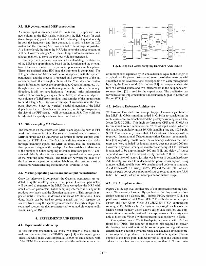
Fig. 2. Proposed Gibbs Sampling Hardware Architecture

of microphones separated by 15 cm, a distance equal to the length ofa typical mobile phone. We created two convolutive mixtures withsimulated room reverberations corresponding to each microphonesby using the Roomsim Matlab toolbox [15]. A comprehensive mix-ture of a desired source and five interferences in the cellphone envi-ronment from [2] is used for the experiments. The qualitative per-formance of the implementation is measured by Signal-to-DistortionRatio (SDR) [16].

4.2. Software Reference Architecture

We have implemented a software prototype of source separation us-ing MRF via Gibbs sampling coded in C. Prior to considering themobile use-case, we benchmarked the prototype running on an IntelXeon X6550 2GHz. This high performance CPU took 31.695 msto run sound source separation on 32 ms of input audio, which isthe smallest granularity given 16 KHz sampling rate and 1024-pointSTFT. This essentially means that at least 64 ms of latency will berequired. International Telecommunication Union’s recommenda-tion [17] regarding mouth-to-ear delay latency indicates that mostusers are “very satisfied” as long as latency does not exceed 200 ms.However, a typical latency or mouth-to-ear delay of LTE networkis assumed to be approximately 160 ms [18], and delay of sourceseparated voice on LTE network easily exceeds 200 ms. This un-acceptable level of latency justifies our interest in custom hardware.Additionally, we need to understand the power consumption, usinga more realistic mobile cpu. We benchmarked code on a simulatedARM Cortex-A9 CPU using GEM5 [19] and McPAT [20]. We esti-mate the peak power consumption of source separation on the ARMto be 3.661 Watts, which is unacceptable for mobile usage.

4.3. FPGA Implementation

Figure 2 is the top level architecture of our proposed streaming hard-ware. We currently have a fully synthesized Verilog version of ourdesign running on a Convey HC-1 hybrid-FPGA platform [21]. Theplatform consists of Intel Xeon 5138 2.13 GHz dual-core host pro-cessor, and four Xilinx Virtex 5 (V5LX330) FPGA coprocessorsrunning at 150 MHz each. The system has a single cache-coherentshared virtual memory which allows easier data transfers and com-munication between the host and the co-processors. Our design wasable to fit on one Virtex 5 with resource utilization shown in Table 1.

Our system uses a 32-bit fixed-point arithmetic with 16 frac-tional bits (Q16). The number of fraction bits required to convertthe floating point arithmetic of the source separation algorithm wasdetermined by checking dynamic range and adequate amount of pre-cision required to produce correct values within the system. The ex-ception to this fixed-point number format is input and output streamvalues that are fractions with magnitude less than 1. To maximize

2479

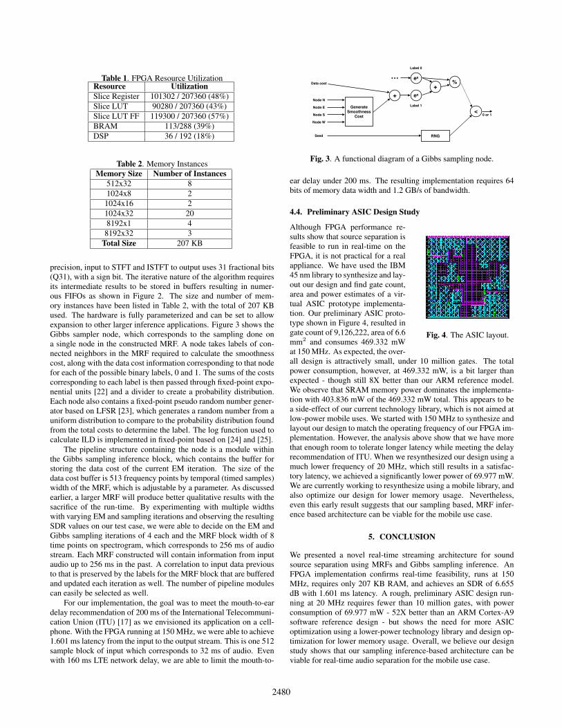
Table 1. FPGA Resource UtilizationResource UtilizationSlice Register 101302 / 207360 (48%)Slice LUT 90280 / 207360 (43%)Slice LUT FF 119300 / 207360 (57%)BRAM 113/288 (39%)DSP 36 / 192 (18%)

Table 2. Memory InstancesMemory Size Number of Instances

512x32 81024x8 2

1024x16 21024x32 208192x1 4

8192x32 3Total Size 207 KB

precision, input to STFT and ISTFT to output uses 31 fractional bits(Q31), with a sign bit. The iterative nature of the algorithm requiresits intermediate results to be stored in buffers resulting in numer-ous FIFOs as shown in Figure 2. The size and number of mem-ory instances have been listed in Table 2, with the total of 207 KBused. The hardware is fully parameterized and can be set to allowexpansion to other larger inference applications. Figure 3 shows theGibbs sampler node, which corresponds to the sampling done ona single node in the constructed MRF. A node takes labels of con-nected neighbors in the MRF required to calculate the smoothnesscost, along with the data cost information corresponding to that nodefor each of the possible binary labels, 0 and 1. The sums of the costscorresponding to each label is then passed through fixed-point expo-nential units [22] and a divider to create a probability distribution.Each node also contains a fixed-point pseudo random number gener-ator based on LFSR [23], which generates a random number from auniform distribution to compare to the probability distribution foundfrom the total costs to determine the label. The log function used tocalculate ILD is implemented in fixed-point based on [24] and [25].

The pipeline structure containing the node is a module withinthe Gibbs sampling inference block, which contains the buffer forstoring the data cost of the current EM iteration. The size of thedata cost buffer is 513 frequency points by temporal (timed samples)width of the MRF, which is adjustable by a parameter. As discussedearlier, a larger MRF will produce better qualitative results with thesacrifice of the run-time. By experimenting with multiple widthswith varying EM and sampling iterations and observing the resultingSDR values on our test case, we were able to decide on the EM andGibbs sampling iterations of 4 each and the MRF block width of 8time points on spectrogram, which corresponds to 256 ms of audiostream. Each MRF constructed will contain information from inputaudio up to 256 ms in the past. A correlation to input data previousto that is preserved by the labels for the MRF block that are bufferedand updated each iteration as well. The number of pipeline modulescan easily be selected as well.

For our implementation, the goal was to meet the mouth-to-eardelay recommendation of 200 ms of the International Telecommuni-cation Union (ITU) [17] as we envisioned its application on a cell-phone. With the FPGA running at 150 MHz, we were able to achieve1.601 ms latency from the input to the output stream. This is one 512sample block of input which corresponds to 32 ms of audio. Evenwith 160 ms LTE network delay, we are able to limit the mouth-to-

Generate!Smoothness

Cost

Node N

Node E

Node S

Node W

+Data cost

ex

RNGSeed

<0 or 1

ex

+

%…

Label 0

Label 1

Fig. 3. A functional diagram of a Gibbs sampling node.

ear delay under 200 ms. The resulting implementation requires 64bits of memory data width and 1.2 GB/s of bandwidth.

4.4. Preliminary ASIC Design Study

Fig. 4. The ASIC layout.

Although FPGA performance re-sults show that source separation isfeasible to run in real-time on theFPGA, it is not practical for a realappliance. We have used the IBM45 nm library to synthesize and lay-out our design and find gate count,area and power estimates of a vir-tual ASIC prototype implementa-tion. Our preliminary ASIC proto-type shown in Figure 4, resulted ingate count of 9,126,222, area of 6.6mm2 and consumes 469.332 mWat 150 MHz. As expected, the over-all design is attractively small, under 10 million gates. The totalpower consumption, however, at 469.332 mW, is a bit larger thanexpected - though still 8X better than our ARM reference model.We observe that SRAM memory power dominates the implementa-tion with 403.836 mW of the 469.332 mW total. This appears to bea side-effect of our current technology library, which is not aimed atlow-power mobile uses. We started with 150 MHz to synthesize andlayout our design to match the operating frequency of our FPGA im-plementation. However, the analysis above show that we have morethat enough room to tolerate longer latency while meeting the delayrecommendation of ITU. When we resynthesized our design using amuch lower frequency of 20 MHz, which still results in a satisfac-tory latency, we achieved a significantly lower power of 69.977 mW.We are currently working to resynthesize using a mobile library, andalso optimize our design for lower memory usage. Nevertheless,even this early result suggests that our sampling based, MRF infer-ence based architecture can be viable for the mobile use case.

5. CONCLUSION

We presented a novel real-time streaming architecture for soundsource separation using MRFs and Gibbs sampling inference. AnFPGA implementation confirms real-time feasibility, runs at 150MHz, requires only 207 KB RAM, and achieves an SDR of 6.655dB with 1.601 ms latency. A rough, preliminary ASIC design run-ning at 20 MHz requires fewer than 10 million gates, with powerconsumption of 69.977 mW - 52X better than an ARM Cortex-A9software reference design - but shows the need for more ASICoptimization using a lower-power technology library and design op-timization for lower memory usage. Overall, we believe our designstudy shows that our sampling inference-based architecture can beviable for real-time audio separation for the mobile use case.

2480

6. REFERENCES

[1] J-F Cardoso, “Blind signal separation: statistical principles,”Proceedings of the IEEE, vol. 86, no. 10, pp. 2009–2025, 1998.

[2] M. Kim, P. Smaragdis, G.G. Ko, and R.A. Rutenbar,“Stereophonic spectrogram segmentation using markov ran-dom fields,” in International Workshop on Machine Learningfor Signal Processing (MLSP). IEEE, 2012.

[3] C. Charoensak and F. Sattar, “A single-chip fpga design forreal-time ica-based blind source separation algorithm,” in Cir-cuits and Systems, 2005. ISCAS 2005. IEEE International Sym-posium on, may 2005, pp. 5822 – 5825 Vol. 6.

[4] Charayaphan Charoensak and Farook Sattar, “Design of low-cost fpga hardware for real-time ica-based blind source separa-tion algorithm,” EURASIP J. Appl. Signal Process., vol. 2005,pp. 3076–3086, Jan. 2005.

[5] K.-K. Shyu, M.-H. Lee, Y.-T. Wu, and P.-L. Lee, “Implemen-tation of pipelined fastica on fpga for real-time blind sourceseparation,” Neural Networks, IEEE Transactions on, vol. 19,no. 6, pp. 958 –970, june 2008.

[6] Vikash K. Mansinghka, Eric M. Jonas, and Joshua B. Tenen-baum, “Stochastic digital circuits for probabilistic infer-ence,” Tech. Rep., Massachussets Institute of Technology,2008, MITCSAIL-TR-2008-069.

[7] Vikash K. Mansinghka and Eric Jonas, “Building fast bayesiancomputing machines out of intentionally stochastic, digitalparts,” CoRR, vol. abs/1402.4914, 2014.

[8] Siyang Wang, Xiangyu Zhang, Yuxuan Li, Ramin Bashizade,Song Yang, Chris Dwyer, and Alvin R. Lebeck, “Acceleratingmarkov random field inference using molecular optical gibbssampling units,” in Proceedings of the International Sympo-sium on Computer Architecture, 2016, ISCA ’16.

[9] Dongzhen Piao, Speeding Up Gibbs Sampling in ProbabilisticOptical Flow, PhD dissertation, Carnegie Mellon University,2014.

[10] V. Kolmogorov, “Convergent tree-reweighted message passingfor energy minimization,” Pattern Analysis and Machine Intel-ligence, IEEE Transactions on, vol. 28, no. 10, pp. 1568–1583,2006.

[11] R. Szeliski, R. Zabih, D. Scharstein, O. Veksler, V. Kol-mogorov, A. Agarwala, M. Tappen, and C. Rother, “A compar-ative study of energy minimization methods for markov ran-dom fields with smoothness-based priors,” Pattern Analysisand Machine Intelligence, IEEE Transactions on, vol. 30, no.6, pp. 1068–1080, 2008.

[12] S. Geman and D. Geman, “Stochastic relaxation, gibbs distri-butions, and the bayesian restoration of images,” Pattern Anal-ysis and Machine Intelligence, IEEE Transactions on, , no. 6,pp. 721–741, 1984.

[13] Yuri Y Boykov and M-P Jolly, “Interactive graph cuts for op-timal boundary & region segmentation of objects in nd im-ages,” in Computer Vision, 2001. ICCV 2001. Proceedings.Eighth IEEE International Conference on. IEEE, 2001, vol. 1,pp. 105–112.

[14] J.S. Garofolo, L.F. Lamel, W. M. Fisher, J.G. Fiscus, D.S. Pal-lett, N.L. Dahlgren, and Zue V., “Timit acoustic-phonetic con-tinuous speech corpus,” Linguistic Data Consortium, 1993.

[15] D. Campbell, K. Palomaki, and G. Brown, “A matlab sim-ulation of” shoebox” room acoustics for use in research andteaching,” Computing and Information Systems, vol. 9, no. 3,pp. 48, 2005.

[16] E. Vincent, R. Gribonval, and C. Fevotte, “Performance mea-surement in blind audio source separation,” Audio, Speech,and Language Processing, IEEE Transactions on, vol. 14, no.4, pp. 1462–1469, 2006.

[17] Telecommunication Standardization Sector of ITU, “Interna-tional telephone connections and circuits -general recommendations on the transmission quality for anentire international telephone connection,” ITU-T Recommen-dation G.114, 2003.

[18] H. Holma and A. Toskala, LTE for UMTS: Evolution to LTE-Advanced, Wiley, 2011.

[19] Nathan Binkert, Bradford Beckmann, Gabriel Black, Steven KReinhardt, Ali Saidi, Arkaprava Basu, Joel Hestness, Derek RHower, Tushar Krishna, Somayeh Sardashti, et al., “The gem5simulator,” ACM SIGARCH Computer Architecture News, vol.39, no. 2, pp. 1–7, 2011.

[20] Sheng Li, Jung Ho Ahn, Richard D Strong, Jay B Brockman,Dean M Tullsen, and Norman P Jouppi, “Mcpat: an inte-grated power, area, and timing modeling framework for multi-core and manycore architectures,” in Proceedings of the 42ndAnnual IEEE/ACM International Symposium on Microarchi-tecture. ACM, 2009, pp. 469–480.

[21] Convey Computer, “The convey hc-1 computer, architectureoverview,” nov. 2008.

[22] Jeremie Detrey and Florent de Dinechin, “Parameterizedfloating-point logarithm and exponential functions for fpgas,”Microprocessors and Microsystems, vol. 31, no. 8, pp. 537–545, 2007.

[23] Thomas E. Tkacik, “A hardware random number generator,” inRevised Papers from the 4th International Workshop on Cryp-tographic Hardware and Embedded Systems, London, UK,UK, 2003, CHES ’02, pp. 450–453, Springer-Verlag.

[24] John N Mitchell, “Computer multiplication and division usingbinary logarithms,” IRE Transactions on Electronic Comput-ers, , no. 4, pp. 512–517, 1962.

[25] Roberto Gutierrez and Javier Valls, “Low cost hardware im-plementation of logarithm approximation,” IEEE Transactionson Very Large Scale Integration (VLSI) Systems, vol. 19, no.12, pp. 2326–2330, 2011.

2481