a biologically inspired approach to feasible …matwbn.icm.edu.pl/ksiazki/amc/amc20/amc2015.pdf ·...

Int. J. Appl. Math. Comput. Sci., 2010, Vol. 20, No. 1, 69–84DOI: 10.2478/v10006-010-0005-7

A BIOLOGICALLY INSPIRED APPROACH TO FEASIBLE GAIT LEARNINGFOR A HEXAPOD ROBOT

DOMINIK BELTER, PIOTR SKRZYPCZYNSKI

Institute of Control and Information EngineeringPoznan University of Technology, ul. Piotrowo 3A, 60–965, Poznan, Poland

e-mail: dominik.belter,[email protected]

The objective of this paper is to develop feasible gait patterns that could be used to control a real hexapod walking robot.These gaits should enable the fastest movement that is possible with the given robot’s mechanics and drives on a flatterrain. Biological inspirations are commonly used in the design of walking robots and their control algorithms. However,legged robots differ significantly from their biological counterparts. Hence we believe that gait patterns should be learnedusing the robot or its simulation model rather than copied from insect behaviour. However, as we have found tahula rasalearning ineffective in this case due to the large and complicated search space, we adopt a different strategy: in a seriesof simulations we show how a progressive reduction of the permissible search space for the leg movements leads to theevolution of effective gait patterns. This strategy enables the evolutionary algorithm to discover proper leg co-ordinationrules for a hexapod robot, using only simple dependencies between the states of the legs and a simple fitness function. Thedependencies used are inspired by typical insect behaviour, although we show that all the introduced rules emerge alsonaturally in the evolved gait patterns. Finally, the gaits evolved in simulations are shown to be effective in experiments ona real walking robot.

Keywords: evolutionary learning, legged robots, gait generation, model identification, reality gap.

1. Introduction

The generation of gaits—the patterns of moving legs inwalking or running—is a fundamental problem for everywalking robot. For multi-legged robots, developing walk-ing patterns is a challenging task, because there are a largenumber of degrees of freedom and therefore the solutionmust be found in a large, multidimensional search/statespace, where useful states are sparsely distributed.

The issues of gait generation have been studied formany years, and there are various approaches to this prob-lem known from the literature (Ridderstrom, 1999). Al-though the generation of adaptive gait patterns has alreadybeen demonstrated in simulated (Kumar and Waldron,1989; Yang, 2009) and real (Fukuoka et al., 2003; Parkerand Mills, 1999) environments, many walking robot con-trollers use gaits programmed by hand. In most cases(particularly for six- and eight-legged walking machines)these gaits are statically stable, i.e., the gait longitudinalstability margin is positive (Song and Waldron, 1989).

Typically, the synthesis of simple, static gaits isbased on a kinematic model of the robot, and the de-signer’s inspiration is taken from biology (Figliolini et al.,

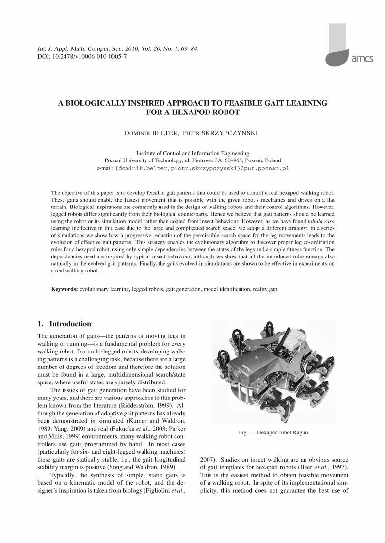
Fig. 1. Hexapod robot Ragno.

2007). Studies on insect walking are an obvious sourceof gait templates for hexapod robots (Beer et al., 1997).This is the easiest method to obtain feasible movementof a walking robot. In spite of its implementational sim-plicity, this method does not guarantee the best use of

dominik.belter,[email protected]

70 D. Belter and P. Skrzypczynski

the robot kinematic and dynamic capabilities. When legco-ordination patterns known from nature are used, someother gaits are excluded by design, only because they havenot been observed in living creatures. Despite the factthat these walking patterns are not used in nature, it isworth verifying whether they are applicable to walkingmachines. Even though insects are simple animals, theyare much more complex than the existing walking robots.An example may be leg specialization found in both in-sects and vertebrates, which is largely ignored in the de-sign of walking robots due to technological and controlissues (Ritzmann et al., 2004). Thus, as it seems to be im-possible to copy even the simplest insect into a robotic de-sign, also movement strategies, including gaits, may dif-fer. We believe that gaits optimized or learned using anactual robot can perform better than their counterparts di-rectly modelled on biological patterns due to their adjust-ment to the specific robot hardware.

To find gait patterns for a walking robot from scratch,the multidimensional space of all possible leg statesshould be examined. The hexapod robot Ragno (Fig. 1)used in this research has 18 degrees of freedom, so in ageneral case 18 reference values for all the active jointshave to be determined in every control cycle. A variety ofmethods exist for solving such a problem, but an evolu-tionary algorithm seems to be appropriate to perform thisdifficult task, due to its ability to provide an approach tothe global solution better than gradient-based analyticalalgorithms, its good explorative properties, and insensi-tivity to the initial parameters.

However, even with an evolutionary technique learn-ing one big task by the robot at once may be hard. A rea-sonable solution to this problem is the supervised learn-ing procedure: a human supervisor defines the whole con-trol framework and evaluates the progress of the learn-ing robot. Such an approach is often called ‘shaping’(Dorigo and Colombetti, 1997). This paradigm wasused successfully in our previous research on GA-basedlearning of fuzzy reactive behaviour for a wheeled robot(Skrzypczynski, 2004b).

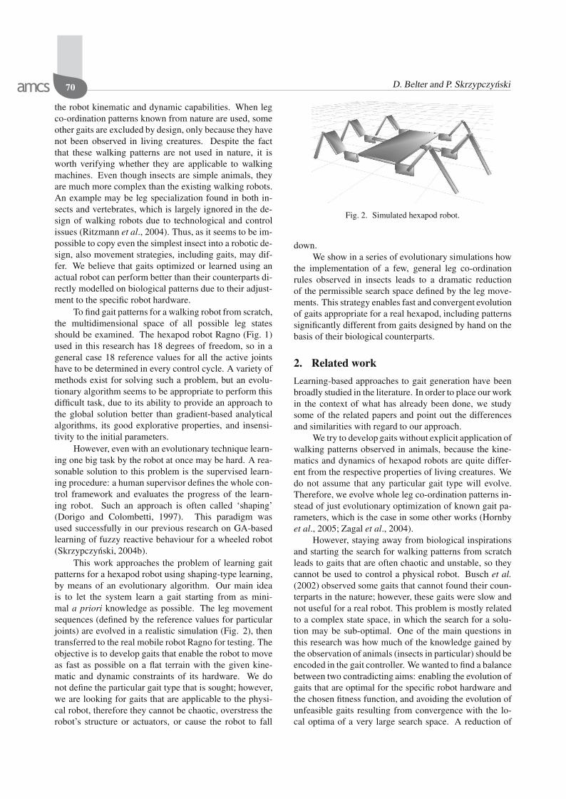
This work approaches the problem of learning gaitpatterns for a hexapod robot using shaping-type learning,by means of an evolutionary algorithm. Our main ideais to let the system learn a gait starting from as mini-mal a priori knowledge as possible. The leg movementsequences (defined by the reference values for particularjoints) are evolved in a realistic simulation (Fig. 2), thentransferred to the real mobile robot Ragno for testing. Theobjective is to develop gaits that enable the robot to moveas fast as possible on a flat terrain with the given kine-matic and dynamic constraints of its hardware. We donot define the particular gait type that is sought; however,we are looking for gaits that are applicable to the physi-cal robot, therefore they cannot be chaotic, overstress therobot’s structure or actuators, or cause the robot to fall

Fig. 2. Simulated hexapod robot.

down.We show in a series of evolutionary simulations how

the implementation of a few, general leg co-ordinationrules observed in insects leads to a dramatic reductionof the permissible search space defined by the leg move-ments. This strategy enables fast and convergent evolutionof gaits appropriate for a real hexapod, including patternssignificantly different from gaits designed by hand on thebasis of their biological counterparts.

2. Related work

Learning-based approaches to gait generation have beenbroadly studied in the literature. In order to place our workin the context of what has already been done, we studysome of the related papers and point out the differencesand similarities with regard to our approach.

We try to develop gaits without explicit application ofwalking patterns observed in animals, because the kine-matics and dynamics of hexapod robots are quite differ-ent from the respective properties of living creatures. Wedo not assume that any particular gait type will evolve.Therefore, we evolve whole leg co-ordination patterns in-stead of just evolutionary optimization of known gait pa-rameters, which is the case in some other works (Hornbyet al., 2005; Zagal et al., 2004).

However, staying away from biological inspirationsand starting the search for walking patterns from scratchleads to gaits that are often chaotic and unstable, so theycannot be used to control a physical robot. Busch et al.(2002) observed some gaits that cannot found their coun-terparts in the nature; however, these gaits were slow andnot useful for a real robot. This problem is mostly relatedto a complex state space, in which the search for a solu-tion may be sub-optimal. One of the main questions inthis research was how much of the knowledge gained bythe observation of animals (insects in particular) should beencoded in the gait controller. We wanted to find a balancebetween two contradicting aims: enabling the evolution ofgaits that are optimal for the specific robot hardware andthe chosen fitness function, and avoiding the evolution ofunfeasible gaits resulting from convergence with the lo-cal optima of a very large search space. A reduction of

A biologically inspired approach to feasible gait learning for a hexapod robot 71

this space comes from excluding a priori some unwantedsolutions (Belter et al., 2008). Niching could be addition-ally incorporated in order to avoid premature convergence(Kowalczuk and Białaszewski, 2006). While it is not op-timal to use copied insect gaits with a robot, and it is nei-ther possible nor feasible to copy the Darwinian evolu-tion (Albiez and Berns, 2004), when trying to reduce thesearch space, it is interesting to take advantage of the rulesand/or constraints that proved to lead to a proper solutionin natural evolution.

We use an evolutionary algorithm to effectivelysearch for optimal gaits. The term ‘evolutionary algo-rithms’ summarizes a family of machine learning andoptimization methods inspired by biological evolution(Holland, 1975) that include (among others) genetic al-gorithms (GAs), genetic programming (GP), and evo-lution strategies (ESs) (Arabas, 2001). Evolving con-trol systems by using genetic algorithms has becomequite popular in the field of robotics (see (Walker etal., 2003) for a survey). Learning and tuning behaviour bymeans of GA was found useful in developing behaviour-based control systems of wheeled mobile robots (e.g.,(Skrzypczynski, 2004a; 2004b).

In the walking machines domain, GA-based meth-ods have been used to evolve gaits for a number of leggedrobots, including hexapods (Barfoot et al., 2006; Gal-lagher et al., 1996; Lewis et al., 1994) and octopods(Jakobi, 1998; Luk et al., 2001). An evolutionary algo-rithm has also been successfully applied in the process ofdeveloping dynamic gaits for four-legged Sony entertain-ment robots (Hornby et al., 2005). Also other learning al-gorithms have already been applied to the gait generationproblem, most notably different variants of the reinforce-ment learning (RL) paradigm. For example, six-leggedGenghis learned to co-ordinate a simple behaviour set re-sulting in a tripod gait (Maes and Brooks, 1990).

In (Kirchner, 1998), Q-learning was used to developswing and stance movements for legs of a hexapod robot.Also Kimura et al. (2001) and Svinin et al. (2001) usedRL to develop motion patterns for a quadruped and anoctopod, respectively. We prefer to use an evolutionaryalgorithm rather than RL, because problems with largestate spaces are known to be hard to solve with foun-dational RL algorithms. While it is possible to decom-pose a priori the search space by enumerating the stati-cally stable robot configurations and eliminating the un-stable ones, an explicit description of the stable configu-rations is not always general and precise enough (Svininet al., 2001). In the system under study such a decomposi-tion might lead to an unnecessary reduction of the admis-sible search space, and it might impact the ability to learnoptimal gaits. Therefore, we prefer to explore the non-decomposed search space, and we require an appropriatelearning algorithm to accomplish this. Although severalresearchers have successfully applied special RL variants

to various robot learning problems involving large statespaces (Tuyls et al., 2003), we have chosen evolution-ary algorithms instead, which can handle complex, non-differentiable search spaces (Goldberg, 1989).

The motivation for using a simulator for learningrobot gaits stems primarily from the fact that try-and-errorlearning using a real robot may be dangerous for the hard-ware. Also, significant effort (recharging of batteries, re-pairs) may be necessary to maintain the real robot dur-ing continuous testing (Maes and Brooks, 1990). Becauseof these problems, real-world experiments can impose aprohibitive time overhead. The number of simulated runsperformed in a given amount of time can be much higherthan that of real experiments. However, any simplifica-tion made in a simulator may be exploited by the learningalgorithm, resulting in a gait pattern, which cannot be re-produced in the real robot. The problem of transferringthe results from a simulation to a real robot has been rec-ognized in the literature (Mataric and Cliff, 1996; Walkeret al., 2003). The system described here crosses the so-called ‘reality gap’ (Jakobi et al., 1995) by using a simu-lator that models the physical characteristics of the robot,including its dynamics, and the way a real robot interactswith the environment.

Although there are known results on gait learningusing physical robots, we prefer learning in simulationdue to reasons related to the aim of this research and thechosen learning method. As stated before, the aim is toevolve gaits that are optimal for the given task and robothardware. Hence, we try to learn walking patterns fromscratch, and we would also like to explore the dynamicstates of the robot, beyond the static stability area. When-ever basic motion patterns are acquired through interac-tion with the environment, the possibility of critical fail-ures increases. The issues of safety during gait learningusing an actual robot are considered by Huber and Gru-pen (1997). One of their safety constraints requires thatthe walking robot should always remain statically stable.Introducing such a constraint eliminates a large, ‘unsafe’portion of the search space but also any possibility to ob-tain gaits that include dynamic states, which is clearlyagainst our aims. On the other hand, whenever dynamicstates are allowed, it is difficult to provide a set of con-straints which will ensure robot safety. Such problemsobviously do not exist in the simulator, where every colli-sion and every excessive force in a joint is detected by thesoftware.

One can argue that using the actual robot to obtainthe reinforcement feedback from the environment shouldcompletely remove the reality gap problem. However, inmost of the works that use physical robots in gait learningthese robots are equipped with special hardware to col-lect the reinforcement signals (Kimura et al., 2001; Maesand Brooks, 1990) or are placed in a completely artificialenvironment like the treadmill setup designed by Barfoot


et al. (2006) to evolve walking gaits. Hence, robots arenot confronted with the real world as it is, because theadditional equipment may cause errors or bias in the rein-forcement signal (e.g., due to wheel slippage) or even in-troduce factors that are not present in the natural environ-ment (Barfoot et al., 2006). Therefore, real robot-basedgait learning systems are not completely free from the re-ality gap problem. However, in the real world, there aresituations that cannot be foreseen, and it is not possibleto program or learn an appropriate set of reactions for it inadvance. As was observed by Kirchner (1998), such prob-lems should be solved by the robot itself during interactionwith the environment, and that is where learning using areal machine should be used. Real robot learning may bealso used for the adaptation of an existing control systemto particular properties of the environment. An example ofsuch a learning system is shown by Chernova and Veloso(2004), where quadruped robots used for robotic socceradapt to a new walking surface.

A well-established paradigm in the evolutionaryrobotics literature is the minimal simulation. The minimalsimulation principle was proposed by Jakobi (1995), whoapplied it to different robots, including an eight-leggedwalking machine (Jakobi, 1998). The same approach isalso used by Svinin et al. (2001), where the minimalsimulation model of an octopod is explained in detail. Incontrast, we use a simulator based on the exact dynamicmodel of the Ragno robot. Researchers using the minimalsimulation approach argue that a learning procedure basedon a model of a robot’s dynamics can be prohibitivelyslow (Jakobi et al., 1995). However, recent advancesin computer speed and the availability of fast, optimizedsoftware ‘engines’ implementing the simulation of real-world physics made such simulators a viable solution forevolutionary robotics. While a minimal simulation may beenough to provide a reinforcement for a wheeled mobilerobot performing a simple navigation task, legged robotsshould explore their dynamics to achieve effective gaits.

The minimal octopod robot model developed in(Svinin et al., 2001) excludes any dynamical effects re-lated to the balancing motions of the body and assumesthat the proper control commands lead to stable configu-rations. Whenever the robot comes into an unstable con-figuration, the command that led to this configuration im-mediately gets a negative reinforcement. Obviously, suchan approach does not permit the evolution of gaits that in-clude dynamic states. As pointed out by Gallagher et al.(1996), who use a simple simulation to evolve gaits for ahexapod robot, an important difference between the simu-lated and the real robot is that the oversimplified simulatedrobot falls down as soon as static stability is lost, whilethe real robot needs time to fall. Observing our results(cf. Fig. 17), one can see that the more elaborated, non-minimal simulator enables the learning system to explorethis fact, and to evolve a fast gait that does not preserve

(a) (b)

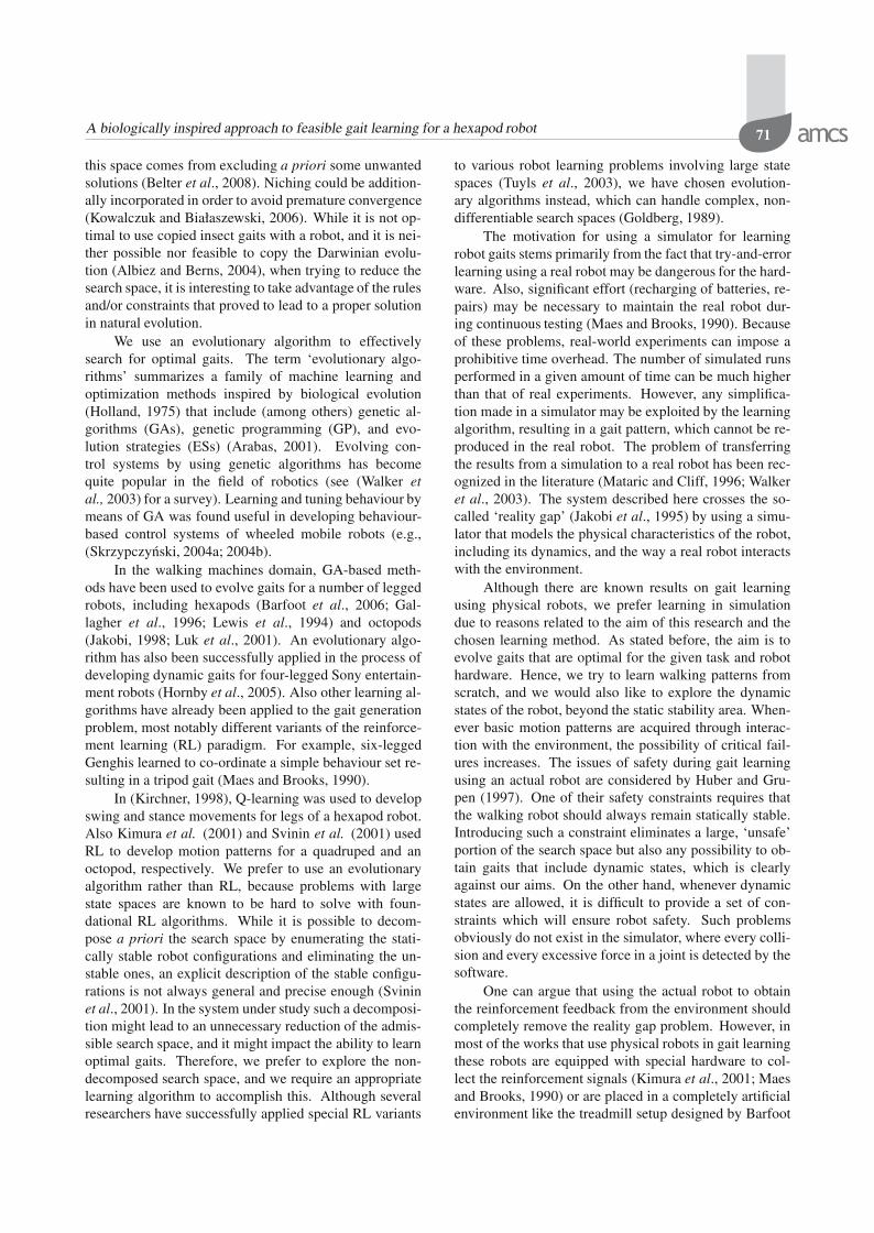
Fig. 3. Robot co-ordinate system and leg numbering (a). Neu-tral position of a leg (b).

the static stability all the time.

3. Experimental setup

3.1. Hexapod robot. The walking robot Ragno (cf.Fig. 1), which was developed in-house, is used in thisresearch. It has six legs. Each leg has three joints thatare driven by integrated servomotors. Figure 3(a) showsa general view of this robot’s mechanics, its local co-ordinate frame and the leg numbering convention used.The robot is 33 cm long and 30 cm wide and weights2.15 kg (without batteries).

The control architecture of the robot is divided intofour layers (Walas et al., 2008). The first one is placedoff-board. It has sufficient resources to compute the ap-propriate control signal for all joints of each leg. The off-board layer sends control commands to the robot. Thecommands include 18 reference values for the leg joints.These reference values are determined as a difference be-tween the desired joint positions and the neutral ones. Theneutral position for a leg is shown in Fig. 3(b) and is de-fined by the vector of the joint angles: [90, 45,−117]T .To change the leg position, the difference between the ref-erence and the neutral position has to be sent to the legjoint controllers. Sending the zero vector for a given legmeans setting this leg to its neutral position.

The second, on-board control layer interprets thesecommands and sends them to the appropriate leg con-trollers. There are six leg controllers that work simulta-neously. They produce control inputs for the integratedservomechanisms of the joints. Each joint has a feedbackfrom its angle position. Additionally, the robot has a dou-ble axis accelerometer and a gyroscope to measure trunkorientation in a 3D space. The on-board and off-boardparts of the control system communicate by means of aBluetooth connection.

The robot has been programmed by hand to walkwith two statically stable gaits: a simple crawl and atripod-like gait. The crawl is used at slow speeds—at mostone leg is transferred at a time. In the tripod gait two setsof three legs each are moved repeatedly. This is the fasteststatically stable gait for a hexapod, and according to Wil-son (1966) it is one of the standard gaits of insects. The


012345

012345

012345

012345

012345

012345

0 mm

10 mm

LEG 1

0 mm

10 mm

0 mm

10 mm

0 mm

10 mm

0 mm

10 mm

LEG 2

LEG 3

LEG 4

LEG 5

0 mm

10 mm

LEG 6

RIG

HT

LE

GS

LE

FT

LE

GS

1 2 3 4 5 6 7 8 Tp

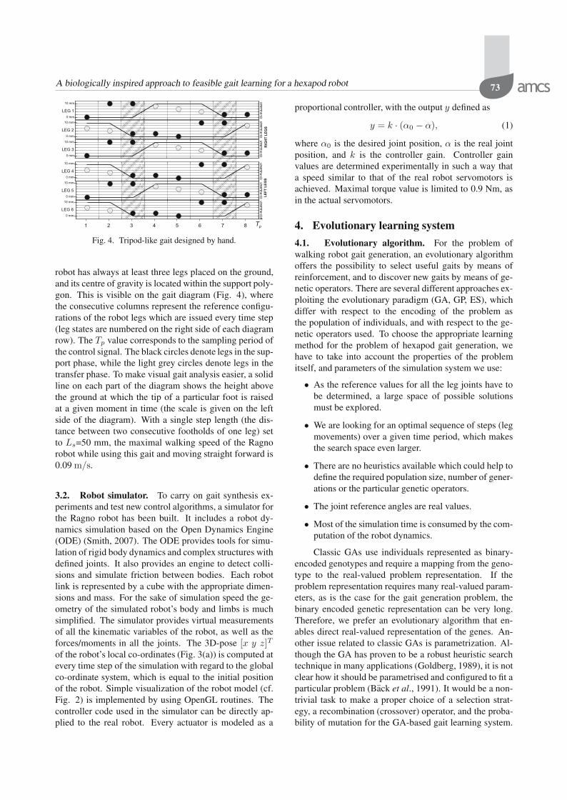
Fig. 4. Tripod-like gait designed by hand.

robot has always at least three legs placed on the ground,and its centre of gravity is located within the support poly-gon. This is visible on the gait diagram (Fig. 4), wherethe consecutive columns represent the reference configu-rations of the robot legs which are issued every time step(leg states are numbered on the right side of each diagramrow). The Tp value corresponds to the sampling period ofthe control signal. The black circles denote legs in the sup-port phase, while the light grey circles denote legs in thetransfer phase. To make visual gait analysis easier, a solidline on each part of the diagram shows the height abovethe ground at which the tip of a particular foot is raisedat a given moment in time (the scale is given on the leftside of the diagram). With a single step length (the dis-tance between two consecutive footholds of one leg) setto Ls=50 mm, the maximal walking speed of the Ragnorobot while using this gait and moving straight forward is0.09 m/s.

3.2. Robot simulator. To carry on gait synthesis ex-periments and test new control algorithms, a simulator forthe Ragno robot has been built. It includes a robot dy-namics simulation based on the Open Dynamics Engine(ODE) (Smith, 2007). The ODE provides tools for simu-lation of rigid body dynamics and complex structures withdefined joints. It also provides an engine to detect colli-sions and simulate friction between bodies. Each robotlink is represented by a cube with the appropriate dimen-sions and mass. For the sake of simulation speed the ge-ometry of the simulated robot’s body and limbs is muchsimplified. The simulator provides virtual measurementsof all the kinematic variables of the robot, as well as theforces/moments in all the joints. The 3D-pose [x y z]T

of the robot’s local co-ordinates (Fig. 3(a)) is computed atevery time step of the simulation with regard to the globalco-ordinate system, which is equal to the initial positionof the robot. Simple visualization of the robot model (cf.Fig. 2) is implemented by using OpenGL routines. Thecontroller code used in the simulator can be directly ap-plied to the real robot. Every actuator is modeled as a

proportional controller, with the output y defined as

y = k · (α0 − α), (1)

where α0 is the desired joint position, α is the real jointposition, and k is the controller gain. Controller gainvalues are determined experimentally in such a way thata speed similar to that of the real robot servomotors isachieved. Maximal torque value is limited to 0.9 Nm, asin the actual servomotors.

4. Evolutionary learning system

4.1. Evolutionary algorithm. For the problem ofwalking robot gait generation, an evolutionary algorithmoffers the possibility to select useful gaits by means ofreinforcement, and to discover new gaits by means of ge-netic operators. There are several different approaches ex-ploiting the evolutionary paradigm (GA, GP, ES), whichdiffer with respect to the encoding of the problem asthe population of individuals, and with respect to the ge-netic operators used. To choose the appropriate learningmethod for the problem of hexapod gait generation, wehave to take into account the properties of the problemitself, and parameters of the simulation system we use:

• As the reference values for all the leg joints have tobe determined, a large space of possible solutionsmust be explored.

• We are looking for an optimal sequence of steps (legmovements) over a given time period, which makesthe search space even larger.

• There are no heuristics available which could help todefine the required population size, number of gener-ations or the particular genetic operators.

• The joint reference angles are real values.

• Most of the simulation time is consumed by the com-putation of the robot dynamics.

Classic GAs use individuals represented as binary-encoded genotypes and require a mapping from the geno-type to the real-valued problem representation. If theproblem representation requires many real-valued param-eters, as is the case for the gait generation problem, thebinary encoded genetic representation can be very long.Therefore, we prefer an evolutionary algorithm that en-ables direct real-valued representation of the genes. An-other issue related to classic GAs is parametrization. Al-though the GA has proven to be a robust heuristic searchtechnique in many applications (Goldberg, 1989), it is notclear how it should be parametrised and configured to fit aparticular problem (Back et al., 1991). It would be a non-trivial task to make a proper choice of a selection strat-egy, a recombination (crossover) operator, and the proba-bility of mutation for the GA-based gait learning system.


INITIALIZATION

fitness evaluationfor everyindividual

randomly selecttwo individuals

meeting

mutation -new individual

created

stopcondition

reproduction

competition -worse is removed

fitnessevaluation

reproduction -two new

individuals created

STOP

NO

YES

YESNO

NO YES

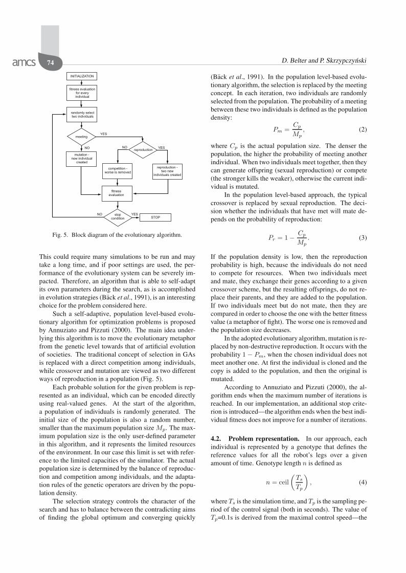
Fig. 5. Block diagram of the evolutionary algorithm.

This could require many simulations to be run and maytake a long time, and if poor settings are used, the per-formance of the evolutionary system can be severely im-pacted. Therefore, an algorithm that is able to self-adaptits own parameters during the search, as is accomplishedin evolution strategies (Back et al., 1991), is an interestingchoice for the problem considered here.

Such a self-adaptive, population level-based evolu-tionary algorithm for optimization problems is proposedby Annuziato and Pizzuti (2000). The main idea under-lying this algorithm is to move the evolutionary metaphorfrom the genetic level towards that of artificial evolutionof societies. The traditional concept of selection in GAsis replaced with a direct competition among individuals,while crossover and mutation are viewed as two differentways of reproduction in a population (Fig. 5).

Each probable solution for the given problem is rep-resented as an individual, which can be encoded directlyusing real-valued genes. At the start of the algorithm,a population of individuals is randomly generated. Theinitial size of the population is also a random number,smaller than the maximum population size Mp. The max-imum population size is the only user-defined parameterin this algorithm, and it represents the limited resourcesof the environment. In our case this limit is set with refer-ence to the limited capacities of the simulator. The actualpopulation size is determined by the balance of reproduc-tion and competition among individuals, and the adapta-tion rules of the genetic operators are driven by the popu-lation density.

The selection strategy controls the character of thesearch and has to balance between the contradicting aimsof finding the global optimum and converging quickly

(Back et al., 1991). In the population level-based evolu-tionary algorithm, the selection is replaced by the meetingconcept. In each iteration, two individuals are randomlyselected from the population. The probability of a meetingbetween these two individuals is defined as the populationdensity:

Pm =Cp

Mp, (2)

where Cp is the actual population size. The denser thepopulation, the higher the probability of meeting anotherindividual. When two individuals meet together, then theycan generate offspring (sexual reproduction) or compete(the stronger kills the weaker), otherwise the current indi-vidual is mutated.

In the population level-based approach, the typicalcrossover is replaced by sexual reproduction. The deci-sion whether the individuals that have met will mate de-pends on the probability of reproduction:

Pr = 1 − Cp

Mp. (3)

If the population density is low, then the reproductionprobability is high, because the individuals do not needto compete for resources. When two individuals meetand mate, they exchange their genes according to a givencrossover scheme, but the resulting offsprings, do not re-place their parents, and they are added to the population.If two individuals meet but do not mate, then they arecompared in order to choose the one with the better fitnessvalue (a metaphor of fight). The worse one is removed andthe population size decreases.

In the adopted evolutionary algorithm, mutation is re-placed by non-destructive reproduction. It occurs with theprobability 1 − Pm, when the chosen individual does notmeet another one. At first the individual is cloned and thecopy is added to the population, and then the original ismutated.

According to Annuziato and Pizzuti (2000), the al-gorithm ends when the maximum number of iterations isreached. In our implementation, an additional stop crite-rion is introduced—the algorithm ends when the best indi-vidual fitness does not improve for a number of iterations.

4.2. Problem representation. In our approach, eachindividual is represented by a genotype that defines thereference values for all the robot’s legs over a givenamount of time. Genotype length n is defined as

n = ceil(

Ts

Tp

), (4)

where Ts is the simulation time, and Tp is the sampling pe-riod of the control signal (both in seconds). The value ofTp=0.1s is derived from the maximal control speed—the


(a)

(b)

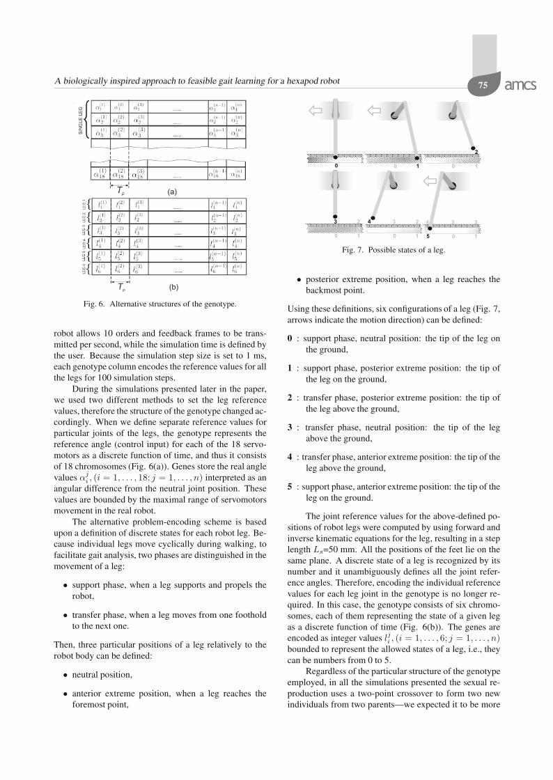
Fig. 6. Alternative structures of the genotype.

robot allows 10 orders and feedback frames to be trans-mitted per second, while the simulation time is defined bythe user. Because the simulation step size is set to 1 ms,each genotype column encodes the reference values for allthe legs for 100 simulation steps.

During the simulations presented later in the paper,we used two different methods to set the leg referencevalues, therefore the structure of the genotype changed ac-cordingly. When we define separate reference values forparticular joints of the legs, the genotype represents thereference angle (control input) for each of the 18 servo-motors as a discrete function of time, and thus it consistsof 18 chromosomes (Fig. 6(a)). Genes store the real anglevalues αj

i , (i = 1, . . . , 18; j = 1, . . . , n) interpreted as anangular difference from the neutral joint position. Thesevalues are bounded by the maximal range of servomotorsmovement in the real robot.

The alternative problem-encoding scheme is basedupon a definition of discrete states for each robot leg. Be-cause individual legs move cyclically during walking, tofacilitate gait analysis, two phases are distinguished in themovement of a leg:

• support phase, when a leg supports and propels therobot,

• transfer phase, when a leg moves from one footholdto the next one.

Then, three particular positions of a leg relatively to therobot body can be defined:

• neutral position,

• anterior extreme position, when a leg reaches theforemost point,

0 0 1

0 1

234

0 1

23

0 1

234

5

0 1

2

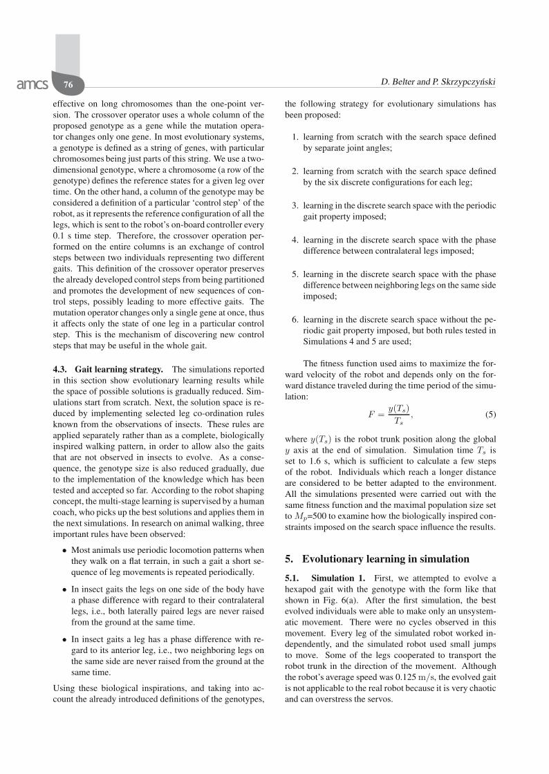
Fig. 7. Possible states of a leg.

• posterior extreme position, when a leg reaches thebackmost point.

Using these definitions, six configurations of a leg (Fig. 7,arrows indicate the motion direction) can be defined:

0 : support phase, neutral position: the tip of the leg onthe ground,

1 : support phase, posterior extreme position: the tip ofthe leg on the ground,

2 : transfer phase, posterior extreme position: the tip ofthe leg above the ground,

3 : transfer phase, neutral position: the tip of the legabove the ground,

4 : transfer phase, anterior extreme position: the tip of theleg above the ground,

5 : support phase, anterior extreme position: the tip of theleg on the ground.

The joint reference values for the above-defined po-sitions of robot legs were computed by using forward andinverse kinematic equations for the leg, resulting in a steplength Ls=50 mm. All the positions of the feet lie on thesame plane. A discrete state of a leg is recognized by itsnumber and it unambiguously defines all the joint refer-ence angles. Therefore, encoding the individual referencevalues for each leg joint in the genotype is no longer re-quired. In this case, the genotype consists of six chromo-somes, each of them representing the state of a given legas a discrete function of time (Fig. 6(b)). The genes areencoded as integer values lji , (i = 1, . . . , 6; j = 1, . . . , n)bounded to represent the allowed states of a leg, i.e., theycan be numbers from 0 to 5.

Regardless of the particular structure of the genotypeemployed, in all the simulations presented the sexual re-production uses a two-point crossover to form two newindividuals from two parents—we expected it to be more


effective on long chromosomes than the one-point ver-sion. The crossover operator uses a whole column of theproposed genotype as a gene while the mutation opera-tor changes only one gene. In most evolutionary systems,a genotype is defined as a string of genes, with particularchromosomes being just parts of this string. We use a two-dimensional genotype, where a chromosome (a row of thegenotype) defines the reference states for a given leg overtime. On the other hand, a column of the genotype may beconsidered a definition of a particular ‘control step’ of therobot, as it represents the reference configuration of all thelegs, which is sent to the robot’s on-board controller every0.1 s time step. Therefore, the crossover operation per-formed on the entire columns is an exchange of controlsteps between two individuals representing two differentgaits. This definition of the crossover operator preservesthe already developed control steps from being partitionedand promotes the development of new sequences of con-trol steps, possibly leading to more effective gaits. Themutation operator changes only a single gene at once, thusit affects only the state of one leg in a particular controlstep. This is the mechanism of discovering new controlsteps that may be useful in the whole gait.

4.3. Gait learning strategy. The simulations reportedin this section show evolutionary learning results whilethe space of possible solutions is gradually reduced. Sim-ulations start from scratch. Next, the solution space is re-duced by implementing selected leg co-ordination rulesknown from the observations of insects. These rules areapplied separately rather than as a complete, biologicallyinspired walking pattern, in order to allow also the gaitsthat are not observed in insects to evolve. As a conse-quence, the genotype size is also reduced gradually, dueto the implementation of the knowledge which has beentested and accepted so far. According to the robot shapingconcept, the multi-stage learning is supervised by a humancoach, who picks up the best solutions and applies them inthe next simulations. In research on animal walking, threeimportant rules have been observed:

• Most animals use periodic locomotion patterns whenthey walk on a flat terrain, in such a gait a short se-quence of leg movements is repeated periodically.

• In insect gaits the legs on one side of the body havea phase difference with regard to their contralaterallegs, i.e., both laterally paired legs are never raisedfrom the ground at the same time.

• In insect gaits a leg has a phase difference with re-gard to its anterior leg, i.e., two neighboring legs onthe same side are never raised from the ground at thesame time.

Using these biological inspirations, and taking into ac-count the already introduced definitions of the genotypes,

the following strategy for evolutionary simulations hasbeen proposed:

1. learning from scratch with the search space definedby separate joint angles;

2. learning from scratch with the search space definedby the six discrete configurations for each leg;

3. learning in the discrete search space with the periodicgait property imposed;

4. learning in the discrete search space with the phasedifference between contralateral legs imposed;

5. learning in the discrete search space with the phasedifference between neighboring legs on the same sideimposed;

6. learning in the discrete search space without the pe-riodic gait property imposed, but both rules tested inSimulations 4 and 5 are used;

The fitness function used aims to maximize the for-ward velocity of the robot and depends only on the for-ward distance traveled during the time period of the simu-lation:

F =y(Ts)Ts

, (5)

where y(Ts) is the robot trunk position along the globaly axis at the end of simulation. Simulation time Ts isset to 1.6 s, which is sufficient to calculate a few stepsof the robot. Individuals which reach a longer distanceare considered to be better adapted to the environment.All the simulations presented were carried out with thesame fitness function and the maximal population size setto Mp=500 to examine how the biologically inspired con-straints imposed on the search space influence the results.

5. Evolutionary learning in simulation

5.1. Simulation 1. First, we attempted to evolve ahexapod gait with the genotype with the form like thatshown in Fig. 6(a). After the first simulation, the bestevolved individuals were able to make only an unsystem-atic movement. There were no cycles observed in thismovement. Every leg of the simulated robot worked in-dependently, and the simulated robot used small jumpsto move. Some of the legs cooperated to transport therobot trunk in the direction of the movement. Althoughthe robot’s average speed was 0.125 m/s, the evolved gaitis not applicable to the real robot because it is very chaoticand can overstress the servos.


012345

012345

012345

012345

012345

012345

0 mm

10 mm

LEG 1

0 mm

10 mm

0 mm

10 mm

0 mm

10 mm

0 mm

10 mm

LEG 2

LEG 3

LEG 4

LEG 5

0 mm

10 mm

LEG 6

RIG

HT

LE

GS

LE

FT

LE

GS

1 2 3 4 5 6 7 8 9 Tp10 11 12 13 14 15

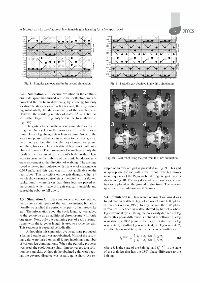
Fig. 8. Irregular gait obtained in the second simulation.

5.2. Simulation 2. Because evolution in the continu-ous state space had turned out to be ineffective, we ap-proached the problem differently, by allowing for onlysix discrete states for each robot leg and, thus, by reduc-ing substantially the dimensionality of the search space.However, the resulting number of states, 66 = 46656, isstill rather large. The genotype has the form shown inFig. 6(b).

The gaits obtained in the second simulation were alsoirregular. No cycles in the movement of the legs werefound. Every leg changes its role in walking. Some of thelegs have phase difference in relation to the others, as inthe tripod gait, but after a while they change their phase,and then, for example, contralateral legs work without aphase difference. The movement of some legs is only theresult of the movement of the robot’s body, as these legswork to preserve the stability of the trunk, but do not gen-erate movement in the direction of walking. The averagespeed achieved in simulation with this way of walking was0.073 m/s, and this gait was still not applicable to thereal robot. This is visible on the gait diagram (Fig. 8),which shows some control steps (denoted with a slantedbackground), where fewer than three legs are placed onthe ground, which made this gait statically unstable andcaused the robot to fall down.

5.3. Simulation 3. In the next experiment, we retainedthe discrete state space of the leg movements, but addi-tionally we applied the periodic property of an insect-likegait. The information about the cycle length lc was addedto the genotype as an additional chromosome with onlyone gene. Now, only the beginning part of each chromo-some, with the lc-genes length, is used to evolve the gait.This sequence is repeated periodically.

Although in this simulation cyclic gaits are produced,a fast and stable gait was not obtained. Most of the result-ing gaits were based on small jumps involving a numberof various leg combinations. When the periodic propertywas used, the evolutionary algorithm converged to a solu-tion very quickly. Although the obtained gaits were regu-lar, the covered distance was usually quite short. An ex-

012345

012345

012345

012345

012345

012345

RIG

HT

LE

GS

LE

FT

LE

GS

0 mm

10 mm

LEG 1

0 mm

10 mm

0 mm

10 mm

0 mm

10 mm

0 mm

10 mm

LEG 2

LEG 3

LEG 4

LEG 5

0 mm

10 mm

LEG 6

1 2 3 4 5 6 7 8 9 Tp10 11 12 13 14 15

Fig. 9. Periodic gait obtained in the third simulation.

Fig. 10. Real robot using the gait from the third simulation.

ample of an evolved gait is presented in Fig. 9. This gaitis appropriate for use with a real robot. The leg move-ment sequence of the Ragno robot during one gait cycle isshown in Fig. 10. The grey dots indicate those legs, whosetips were placed on the ground in due time. The averagespeed in this simulation was 0.08 m/s.

5.4. Simulation 4. In research on insect walking it wasfound that contralateral legs of an insect have 180 phasedifference (Wilson, 1966). In a cyclic gait, the 180 phasedifference is defined as a state shifted by half of a wholeleg movement cycle. Using the previously defined six legstates, this phase difference is defined as follows: if a legis in state 0, a 180 phase shifted leg is in state 3; if a legis in state 1, a shifted leg is in state 4; if a leg is in state 2,a shifted leg is in state 5, etc., which can be written as

l+180k =

li + 3, for li ≤ 2,li − 3, for li > 2,

(6)

where li is the state of the i-th leg, and l+180k is the state

of the k-th leg that has the 180 phase difference to thei-th leg.


......

......

......

5

......

......

......

0 14 4 0 1 4 0 14 4 0 1 4 0 1

5 14 4 5 1 4 14 4 1 4 1

0 14 4 0 1 4 0 14 4 0 1 4 0 1

1 3 4 1 3 4 1 3 4

1 3 4 1 3 4 1 3 4

1 2 4 1 2 4 1 2 4

012345

012345

012345

012345

012345

012345

1 2 3 4 5 6 7 8 9

0 mm

10 mm

LEG 1

0 mm

10 mm

0 mm

10 mm

0 mm

10 mm

0 mm

10 mm

LEG 2

LEG 3

LEG 4

LEG 5

0 mm

10 mm

LEG 6

RIG

HT

LE

GS

LE

FT

LE

GS

1 2 3 4 5 6 7 8 9 n

3

Tp

ev

olv

ed

ge

no

typ

e

lc

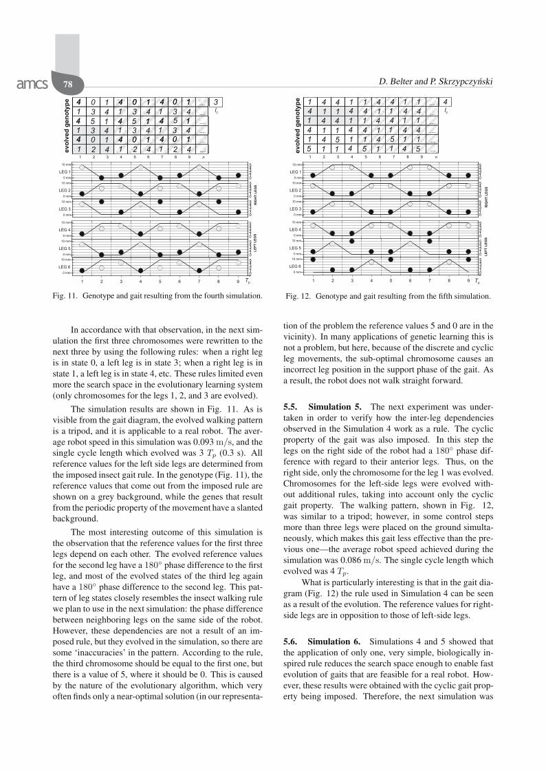
Fig. 11. Genotype and gait resulting from the fourth simulation.

In accordance with that observation, in the next sim-ulation the first three chromosomes were rewritten to thenext three by using the following rules: when a right legis in state 0, a left leg is in state 3; when a right leg is instate 1, a left leg is in state 4, etc. These rules limited evenmore the search space in the evolutionary learning system(only chromosomes for the legs 1, 2, and 3 are evolved).

The simulation results are shown in Fig. 11. As isvisible from the gait diagram, the evolved walking patternis a tripod, and it is applicable to a real robot. The aver-age robot speed in this simulation was 0.093 m/s, and thesingle cycle length which evolved was 3 Tp (0.3 s). Allreference values for the left side legs are determined fromthe imposed insect gait rule. In the genotype (Fig. 11), thereference values that come out from the imposed rule areshown on a grey background, while the genes that resultfrom the periodic property of the movement have a slantedbackground.

The most interesting outcome of this simulation isthe observation that the reference values for the first threelegs depend on each other. The evolved reference valuesfor the second leg have a 180 phase difference to the firstleg, and most of the evolved states of the third leg againhave a 180 phase difference to the second leg. This pat-tern of leg states closely resembles the insect walking rulewe plan to use in the next simulation: the phase differencebetween neighboring legs on the same side of the robot.However, these dependencies are not a result of an im-posed rule, but they evolved in the simulation, so there aresome ‘inaccuracies’ in the pattern. According to the rule,the third chromosome should be equal to the first one, butthere is a value of 5, where it should be 0. This is causedby the nature of the evolutionary algorithm, which veryoften finds only a near-optimal solution (in our representa-

012345

012345

012345

012345

012345

012345

1 2 3 4 5 6 7 8 9

RIG

HT

LE

GS

LE

FT

LE

GS

0 mm

10 mm

LEG 1

0 mm

10 mm

0 mm

10 mm

0 mm

10 mm

0 mm

10 mm

LEG 2

LEG 3

LEG 4

LEG 5

0 mm

10 mm

LEG 6

......

......

......

......

......

......

4 4 1 1 4 4 1 11

4 1 1 4 4 1 1 4 4

4 4 1 1 4 4 1 11

4 1 1 4 4 1 1 4 4

4 5 1 1 4 5 1 11

5 1 1 4 5 1 1 4 51 2 3 4 5 6 7 8 9 n

4

Tp

ev

olv

ed

ge

no

typ

e

lc

Fig. 12. Genotype and gait resulting from the fifth simulation.

tion of the problem the reference values 5 and 0 are in thevicinity). In many applications of genetic learning this isnot a problem, but here, because of the discrete and cyclicleg movements, the sub-optimal chromosome causes anincorrect leg position in the support phase of the gait. Asa result, the robot does not walk straight forward.

5.5. Simulation 5. The next experiment was under-taken in order to verify how the inter-leg dependenciesobserved in the Simulation 4 work as a rule. The cyclicproperty of the gait was also imposed. In this step thelegs on the right side of the robot had a 180 phase dif-ference with regard to their anterior legs. Thus, on theright side, only the chromosome for the leg 1 was evolved.Chromosomes for the left-side legs were evolved with-out additional rules, taking into account only the cyclicgait property. The walking pattern, shown in Fig. 12,was similar to a tripod; however, in some control stepsmore than three legs were placed on the ground simulta-neously, which makes this gait less effective than the pre-vious one—the average robot speed achieved during thesimulation was 0.086 m/s. The single cycle length whichevolved was 4 Tp.

What is particularly interesting is that in the gait dia-gram (Fig. 12) the rule used in Simulation 4 can be seenas a result of the evolution. The reference values for right-side legs are in opposition to those of left-side legs.

5.6. Simulation 6. Simulations 4 and 5 showed thatthe application of only one, very simple, biologically in-spired rule reduces the search space enough to enable fastevolution of gaits that are feasible for a real robot. How-ever, these results were obtained with the cyclic gait prop-erty being imposed. Therefore, the next simulation was


012345

012345

012345

012345

012345

012345

1 2 3 4 5 6 7 8 9

0 mm

10 mm

LEG 1

0 mm

10 mm

0 mm

10 mm

0 mm

10 mm

0 mm

10 mm

LEG 2

LEG 3

LEG 4

LEG 5

0 mm

10 mm

LEG 6

RIG

HT

LE

GS

LE

FT

LE

GS

......

......

......

......

......

......

4 54 1 1 4 4 54 2

1 1 2 4 4 5 1 1 2

4 54 1 1 4 4 54 2

4 54 1 1 4 4 54 2

1 1 2 4 4 5 1 1 2

1 1 2 4 4 5 1 1 2

1 2 3 4 5 6 7 8 9 n

Tp

ev

olv

ed

ge

no

typ

e

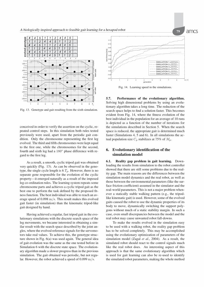
Fig. 13. Genotype and gait resulting from the sixth simulation.

conceived in order to verify the assertion on the cyclic, re-peated control steps. In this simulation both rules testedpreviously were used, apart from the periodic gait con-dition. Only the chromosome representing the first legevolved. The third and fifth chromosomes were kept equalto the first one, while the chromosomes for the second,fourth and sixth leg had a 180 phase difference with re-gard to the first leg.

As a result, a smooth, cyclic tripod gait was obtainedvery quickly (Fig. 13). As can be observed in the geno-type, the single cycle length is 6 Tp. However, there is noseparate gene responsible for the evolution of the cyclicproperty—it emerged naturally as a result of the imposedleg co-ordination rules. The learning system repeats somechromosome parts and achieves a cyclic tripod gait as thebest one to perform the task defined by the proposed fit-ness function. The best individual was able to reach an av-erage speed of 0.098 m/s. This result makes this evolvedgait faster (in simulation) than the kinematic tripod-likegait designed by hand.

Having achieved a regular, fast tripod gait in the evo-lutionary simulations with the discrete search space of theleg movements, we became interested in obtaining a sim-ilar result with the search space described by the joint an-gles, where the evolved reference signals for the servomo-tors take real values. To achieve this, the genotype struc-ture shown in Fig. 6(a) was used again. The general ideaof gait evolution was the same as the one tested before inSimulation 6 with the discrete state space. The evolution-ary algorithm made a slower progress than in the previoussimulation. The gait obtained was periodic, but not regu-lar. However, the robot achieved a speed of 0.099 m/s.

0 1 2 3 4 5 6 7 8 9 x 10

0.02

0.03

0.04

0.05

0.06

0.07

0.08

0.09

generation

bestfitn

ess

[m/s

]

0.10

0.11

0.01

SIMULATION 1

SIMULATION 2

SIMULATION 3

SIMULATION 4

SIMULATION 5

SIMULATION 6

CONTINUOUSSEARCH SPACE

DISCRETESEARCH SPACE





Fig. 14. Learning speed in the simulations.

5.7. Performance of the evolutionary algorithm.Solving high dimensional problems by using an evolu-tionary algorithm takes a long time. The reduction of thesearch space helps to find a solution faster. This becomesevident from Fig. 14, where the fitness evolution of thebest individual in the population for an average of 10 runsis depicted as a function of the number of iterations forthe simulations described in Section 5. When the searchspace is reduced, the appropriate gait is determined muchfaster (Simulations 4, 5 and 6). In all simulations the ac-tual population size Cp stabilizes at 75% of Mp.

6. Evolutionary identification of thesimulation model

6.1. Reality gap problem in gait learning. Down-loading the results from simulation to the robot controllershowed that there are still some problems due to the real-ity gap. The main reasons are the differences between thesimulation model dynamics and the real robot, as well asthose between the environmental parameters (like the sur-face friction coefficient) assumed in the simulator and thereal-world parameters. This is not a major problem when-ever a statically stable walking pattern (e.g., the tripod-like kinematic gait) is used. However, some of the evolvedgaits caused the robot to use the dynamic properties of itsbody to move, dynamically switching the support poly-gons without much of a static stability margin. In such acase, even small discrepancies between the model and thereal robot may cause unwanted robot fall-downs.

To make the results evolved in the simulation easyto be used with a walking robot, the reality gap problemhas to be solved completely. This may be accomplishedusing the evolutionary optimization of parameters of thesimulation model (Zagal et al., 2004). As a result, thesimulated robot should react to the control signals muchlike the real robot does. An interesting aspect of thisapproach is that the same evolutionary algorithm whichis used for gait learning can also be re-used to identifythe simulated robot parameters, making the whole method


more effective from the point of view of the programmingeffort required to cross the reality gap. Although thereare many system identification techniques used in robotics(Kozlowski, 1998), which are based on exact mathemat-ical models of robots, such a model of a multi-leggedwalking machine, even if identified successfully, wouldbe infeasible for our purposes. We are searching for a setof parameters that enable the much simplified simulatedmodel to mimic the real robot behaviour within the cho-sen class and range of control signals. Thus, we are facinga search/optimization problem rather than a typical iden-tification problem. Evolutionary and other soft comput-ing techniques are known for being well suited to solveproblems belonging to this class, which motivated ourchoice. In parallel we performed the same robot parameteroptimization with a different soft computing technique—particle swarm optimization, which is covered elsewhere(Belter and Skrzypczynski, 2009).

6.2. Parameter identification system. The structureof the Ragno robot simulation model is described by fourparameters: the trunk mass, and the masses of the tibia,femur and coxa links constituting a leg (all legs have thesame parameters). Two additional parameters are relatedto the servomotors. One describes the gain of the con-troller in every joint, and the other defines maximal angu-lar speed of joint movement.

For the identification task, the population level-basedevolutionary algorithm described in Section 4.1 was ap-plied, but with different problem encoding and parame-ters. This time the genotype is one-dimensional, and con-sists of a single chromosome with six genes directly repre-senting the real-valued model parameters. The maximumsize of the population was set to 100 individuals.

The general idea of identification is to find a set ofparameters that jointly minimize the discrepancy betweenthe trajectories of some characteristic points of the robotobserved in simulation and in the real Ragno walking ma-chine. However, for this task the choice of such pointsand their trajectories is not straightforward, because theparameter values we search for manifest themselves mostprominently in different types of movement, which are of-ten dynamic and hard to track in a physical robot.

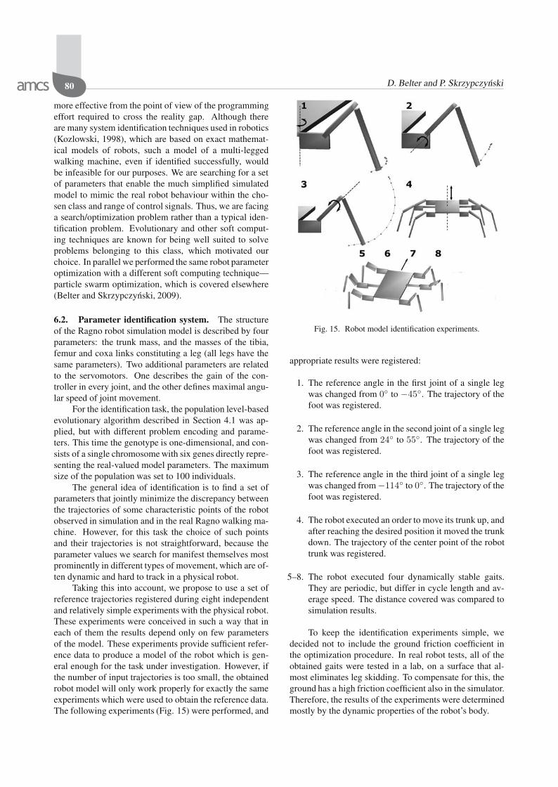
Taking this into account, we propose to use a set ofreference trajectories registered during eight independentand relatively simple experiments with the physical robot.These experiments were conceived in such a way that ineach of them the results depend only on few parametersof the model. These experiments provide sufficient refer-ence data to produce a model of the robot which is gen-eral enough for the task under investigation. However, ifthe number of input trajectories is too small, the obtainedrobot model will only work properly for exactly the sameexperiments which were used to obtain the reference data.The following experiments (Fig. 15) were performed, and

Fig. 15. Robot model identification experiments.

appropriate results were registered:

1. The reference angle in the first joint of a single legwas changed from 0 to −45. The trajectory of thefoot was registered.

2. The reference angle in the second joint of a single legwas changed from 24 to 55. The trajectory of thefoot was registered.

3. The reference angle in the third joint of a single legwas changed from −114 to 0. The trajectory of thefoot was registered.

4. The robot executed an order to move its trunk up, andafter reaching the desired position it moved the trunkdown. The trajectory of the center point of the robottrunk was registered.

5–8. The robot executed four dynamically stable gaits.They are periodic, but differ in cycle length and av-erage speed. The distance covered was compared tosimulation results.

To keep the identification experiments simple, wedecided not to include the ground friction coefficient inthe optimization procedure. In real robot tests, all of theobtained gaits were tested in a lab, on a surface that al-most eliminates leg skidding. To compensate for this, theground has a high friction coefficient also in the simulator.Therefore, the results of the experiments were determinedmostly by the dynamic properties of the robot’s body.


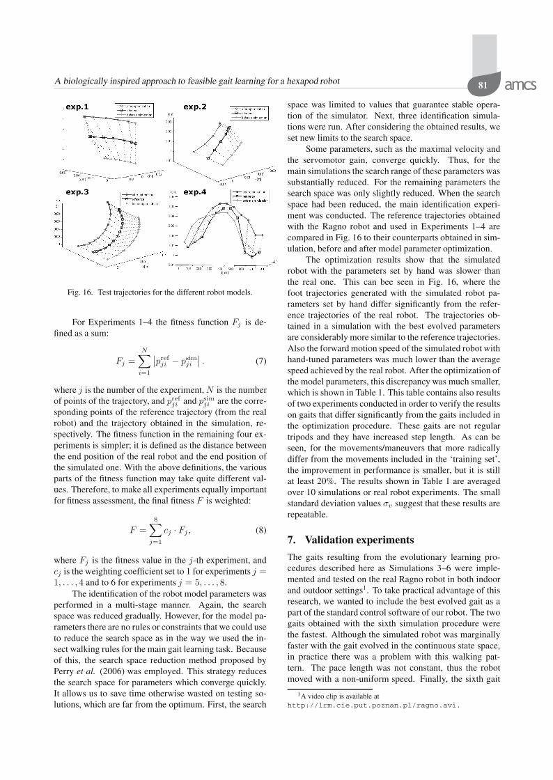
Fig. 16. Test trajectories for the different robot models.

For Experiments 1–4 the fitness function Fj is de-fined as a sum:

Fj =N∑

i=1

∣∣prefji − psim

ji

∣∣ . (7)

where j is the number of the experiment, N is the numberof points of the trajectory, and pref

ji and psimji are the corre-

sponding points of the reference trajectory (from the realrobot) and the trajectory obtained in the simulation, re-spectively. The fitness function in the remaining four ex-periments is simpler; it is defined as the distance betweenthe end position of the real robot and the end position ofthe simulated one. With the above definitions, the variousparts of the fitness function may take quite different val-ues. Therefore, to make all experiments equally importantfor fitness assessment, the final fitness F is weighted:

F =8∑

j=1

cj · Fj , (8)

where Fj is the fitness value in the j-th experiment, andcj is the weighting coefficient set to 1 for experiments j =1, . . . , 4 and to 6 for experiments j = 5, . . . , 8.

The identification of the robot model parameters wasperformed in a multi-stage manner. Again, the searchspace was reduced gradually. However, for the model pa-rameters there are no rules or constraints that we could useto reduce the search space as in the way we used the in-sect walking rules for the main gait learning task. Becauseof this, the search space reduction method proposed byPerry et al. (2006) was employed. This strategy reducesthe search space for parameters which converge quickly.It allows us to save time otherwise wasted on testing so-lutions, which are far from the optimum. First, the search

space was limited to values that guarantee stable opera-tion of the simulator. Next, three identification simula-tions were run. After considering the obtained results, weset new limits to the search space.

Some parameters, such as the maximal velocity andthe servomotor gain, converge quickly. Thus, for themain simulations the search range of these parameters wassubstantially reduced. For the remaining parameters thesearch space was only slightly reduced. When the searchspace had been reduced, the main identification experi-ment was conducted. The reference trajectories obtainedwith the Ragno robot and used in Experiments 1–4 arecompared in Fig. 16 to their counterparts obtained in sim-ulation, before and after model parameter optimization.

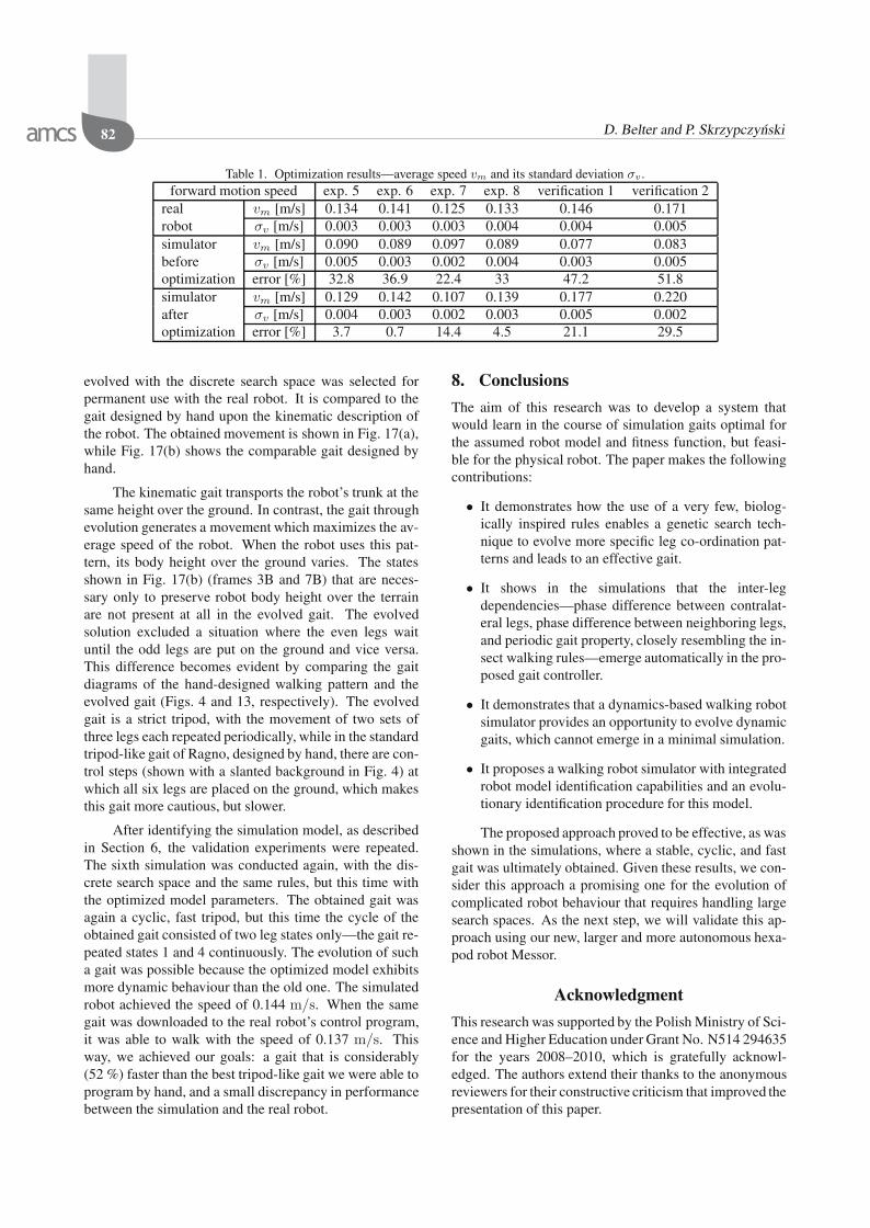
The optimization results show that the simulatedrobot with the parameters set by hand was slower thanthe real one. This can bee seen in Fig. 16, where thefoot trajectories generated with the simulated robot pa-rameters set by hand differ significantly from the refer-ence trajectories of the real robot. The trajectories ob-tained in a simulation with the best evolved parametersare considerably more similar to the reference trajectories.Also the forward motion speed of the simulated robot withhand-tuned parameters was much lower than the averagespeed achieved by the real robot. After the optimization ofthe model parameters, this discrepancy was much smaller,which is shown in Table 1. This table contains also resultsof two experiments conducted in order to verify the resultson gaits that differ significantly from the gaits included inthe optimization procedure. These gaits are not regulartripods and they have increased step length. As can beseen, for the movements/maneuvers that more radicallydiffer from the movements included in the ‘training set’,the improvement in performance is smaller, but it is stillat least 20%. The results shown in Table 1 are averagedover 10 simulations or real robot experiments. The smallstandard deviation values σv suggest that these results arerepeatable.

7. Validation experiments

The gaits resulting from the evolutionary learning pro-cedures described here as Simulations 3–6 were imple-mented and tested on the real Ragno robot in both indoorand outdoor settings1. To take practical advantage of thisresearch, we wanted to include the best evolved gait as apart of the standard control software of our robot. The twogaits obtained with the sixth simulation procedure werethe fastest. Although the simulated robot was marginallyfaster with the gait evolved in the continuous state space,in practice there was a problem with this walking pat-tern. The pace length was not constant, thus the robotmoved with a non-uniform speed. Finally, the sixth gait

1A video clip is available athttp://lrm.cie.put.poznan.pl/ragno.avi.

http://lrm.cie.put.poznan.pl/ragno.avi.


Table 1. Optimization results—average speed vm and its standard deviation σv .forward motion speed exp. 5 exp. 6 exp. 7 exp. 8 verification 1 verification 2

real vm [m/s] 0.134 0.141 0.125 0.133 0.146 0.171robot σv [m/s] 0.003 0.003 0.003 0.004 0.004 0.005simulator vm [m/s] 0.090 0.089 0.097 0.089 0.077 0.083before σv [m/s] 0.005 0.003 0.002 0.004 0.003 0.005optimization error [%] 32.8 36.9 22.4 33 47.2 51.8simulator vm [m/s] 0.129 0.142 0.107 0.139 0.177 0.220after σv [m/s] 0.004 0.003 0.002 0.003 0.005 0.002optimization error [%] 3.7 0.7 14.4 4.5 21.1 29.5

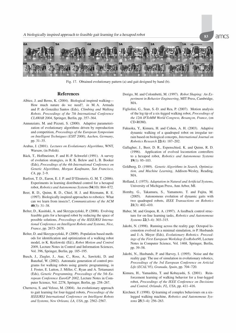
evolved with the discrete search space was selected forpermanent use with the real robot. It is compared to thegait designed by hand upon the kinematic description ofthe robot. The obtained movement is shown in Fig. 17(a),while Fig. 17(b) shows the comparable gait designed byhand.

The kinematic gait transports the robot’s trunk at thesame height over the ground. In contrast, the gait throughevolution generates a movement which maximizes the av-erage speed of the robot. When the robot uses this pat-tern, its body height over the ground varies. The statesshown in Fig. 17(b) (frames 3B and 7B) that are neces-sary only to preserve robot body height over the terrainare not present at all in the evolved gait. The evolvedsolution excluded a situation where the even legs waituntil the odd legs are put on the ground and vice versa.This difference becomes evident by comparing the gaitdiagrams of the hand-designed walking pattern and theevolved gait (Figs. 4 and 13, respectively). The evolvedgait is a strict tripod, with the movement of two sets ofthree legs each repeated periodically, while in the standardtripod-like gait of Ragno, designed by hand, there are con-trol steps (shown with a slanted background in Fig. 4) atwhich all six legs are placed on the ground, which makesthis gait more cautious, but slower.

After identifying the simulation model, as describedin Section 6, the validation experiments were repeated.The sixth simulation was conducted again, with the dis-crete search space and the same rules, but this time withthe optimized model parameters. The obtained gait wasagain a cyclic, fast tripod, but this time the cycle of theobtained gait consisted of two leg states only—the gait re-peated states 1 and 4 continuously. The evolution of sucha gait was possible because the optimized model exhibitsmore dynamic behaviour than the old one. The simulatedrobot achieved the speed of 0.144 m/s. When the samegait was downloaded to the real robot’s control program,it was able to walk with the speed of 0.137 m/s. Thisway, we achieved our goals: a gait that is considerably(52 %) faster than the best tripod-like gait we were able toprogram by hand, and a small discrepancy in performancebetween the simulation and the real robot.

8. Conclusions

The aim of this research was to develop a system thatwould learn in the course of simulation gaits optimal forthe assumed robot model and fitness function, but feasi-ble for the physical robot. The paper makes the followingcontributions:

• It demonstrates how the use of a very few, biolog-ically inspired rules enables a genetic search tech-nique to evolve more specific leg co-ordination pat-terns and leads to an effective gait.

• It shows in the simulations that the inter-legdependencies—phase difference between contralat-eral legs, phase difference between neighboring legs,and periodic gait property, closely resembling the in-sect walking rules—emerge automatically in the pro-posed gait controller.

• It demonstrates that a dynamics-based walking robotsimulator provides an opportunity to evolve dynamicgaits, which cannot emerge in a minimal simulation.

• It proposes a walking robot simulator with integratedrobot model identification capabilities and an evolu-tionary identification procedure for this model.

The proposed approach proved to be effective, as wasshown in the simulations, where a stable, cyclic, and fastgait was ultimately obtained. Given these results, we con-sider this approach a promising one for the evolution ofcomplicated robot behaviour that requires handling largesearch spaces. As the next step, we will validate this ap-proach using our new, larger and more autonomous hexa-pod robot Messor.

Acknowledgment

This research was supported by the Polish Ministry of Sci-ence and Higher Education under Grant No. N514 294635for the years 2008–2010, which is gratefully acknowl-edged. The authors extend their thanks to the anonymousreviewers for their constructive criticism that improved thepresentation of this paper.


Fig. 17. Obtained evolutionary pattern (a) and gait designed by hand (b).

ReferencesAlbiez, J. and Berns, K. (2004). Biological inspired walking—

How much nature do we need?, in M. A. Armadaand P. de Gonzalez Santos (Eds), Climbing and WalkingRobots. Proceedings of the 7th International ConferenceCLAWAR 2004, Springer, Berlin, pp. 357–364.

Annunziato, M. and Pizzuti, S. (2000). Adaptive parameteri-zation of evolutionary algorithms driven by reproductionand competition, Proceedings of the European Symposiumon Intelligent Techniques (ESIT 2000), Aachen, Germany,pp. 31–35.

Arabas, J. (2001). Lectures on Evolutionary Algorithms, WNT,Warsaw, (in Polish).

Back, T., Hoffmeister, F. and H.-P. Schwefel (1991). A surveyof evolution strategies, in R. K. Belew and L. B. Booker(Eds), Proceedings of the 4th International Conference onGenetic Algorithms, Morgan Kaufmann, San Francisco,CA, pp. 2–9.

Barfoot, T. D., Earon, E. J. P. and D’Eleuterio, G. M. T. (2006).Experiments in learning distributed control for a hexapodrobot, Robotics and Autonomous Systems 54(10): 864–872.

Beer, R. D., Quinn, R. D., Chiel, H. J. and Ritzmann, R. E.(1997). Biologically inspired approaches to robotics: Whatcan we learn from insects?, Communications of the ACM40(3): 31–38.

Belter, D., Kasinski, A. and Skrzypczynski, P. (2008). Evolvingfeasible gaits for a hexapod robot by reducing the space ofpossible solutions, Proceedings of the IEEE/RSJ Interna-tional Conference on Intelligent Robots and Systems, Nice,France, pp. 2673–2678.

Belter, D. and Skrzypczynski, P. (2009). Population based meth-ods for identification and optimization of a walking robotmodel, in K. Kozlowski (Ed.), Robot Motion and Control2009, Lecture Notes in Control and Information Sciences,Vol. 396, Springer, Berlin, pp. 185–195.

Busch, J., Ziegler, J., Aue, C., Ross, A., Sawitzki, D. andBanzhaf, W. (2002). Automatic generation of control pro-grams for walking robots using genetic programming, inJ. Foster, E. Lutton, J. Miller, C. Ryan and A. Tettamanzi(Eds), Genetic Programming, Proceedings of the 5th Eu-ropean Conference EuroGP 2002, Lecture Notes in Com-puter Science, Vol. 2278, Springer, Berlin, pp. 258–267.

Chernova, S. and Veloso, M. (2004). An evolutionary approachto gait learning for four-legged robots, Proceedings of theIEEE/RSJ International Conference on Intelligent Robotsand Systems, New Orleans, LA, USA, pp. 2562–2567.

Dorigo, M. and Colombetti, M. (1997). Robot Shaping: An Ex-periment in Behavior Engineering, MIT Press, Cambridge,MA.

Figliolini, G., Stan, S.-D. and Rea, P. (2007). Motion analysisof the leg tip of a six-legged walking robot, Proceedings ofthe 12th IFToMM World Congress, Besancon, France, (onCD-ROM).

Fukuoka, Y., Kimura, H. and Cohen, A. H. (2003). Adaptivedynamic walking of a quadruped robot on irregular ter-rain based on biological concepts, International Journal onRobotics Research 22(4): 187–202.

Gallagher, J., Beer, D. R., Espenschied, K. and Quinn, R. D.(1996). Application of evolved locomotion controllersto a hexapod robot, Robotics and Autonomous Systems19(1): 95–103.

Goldberg, D. (1989). Genetic Algorithms in Search, Optimiza-tion, and Machine Learning, Addison-Wesley, Reading,MA.

Holland, J. (1975). Adaptation in Natural and Artificial Systems,University of Michigan Press, Ann Arbor, MI.

Hornby, G., Takamura, S., Yamamoto, T. and Fujita, M.(2005). Autonomous evolution of dynamic gaits withtwo quadruped robots, IEEE Transactions on Robotics21(3): 402–410.

Huber, M. and Grupen, R. A. (1997). A feedback control struc-ture for on-line learning tasks, Robotics and AutonomousSystems 22(3–4): 303–315.

Jakobi, N. (1998). Running across the reality gap: Octopod lo-comotion evolved in a minimal simulation, in P. Husbandsand J.-A. Meyer (Eds), Evolutionary Robotics. Proceed-ings of the First European Workshop EvoRobot98, LectureNotes in Computer Science, Vol. 1468, Springer, Berlin,pp. 39–58.

Jakobi, N., Husbands, P. and Harvey, I. (1995). Noise and thereality gap: The use of simulation in evolutionary robotics,Proceedings of the 3rd European Conference on ArticialLife (ECAL’95), Granada, Spain, pp. 704–720.

Kimura, H., Yamashita, T. and Kobayashi, S. (2001). Rein-forcement learning of walking behavior for a four-leggedrobot, Proceedings of the IEEE Conference on Decisionsand Control, Orlando, FL, USA, pp. 411–416.

Kirchner, F. (1998). Q-learning of complex behaviours on a six-legged walking machine, Robotics and Autonomous Sys-tems 25(3–4): 256–263.


Kowalczuk, Z. and Białaszewski, T. (2006). Nichingmechanisms in evolutionary computations, InternationalJournal of Applied Mathematics and Computer Science16(1): 59–84.

Kozlowski, K. (1998). Modelling and Identification in Robotics,Springer, Berlin.

Kumar, V. R. and Waldron, K. J. (1989). Adaptive gaitcontrol for a walking robot, Journal of Robotic Systems6(1): 49–76.

Lewis, M., Fagg, A. and Bekey, G. (1994). Genetic algorithmsfor gait synthesis in a hexapod robot, in Y. Zheng (Ed.), Re-cent Trends in Mobile Robots, World Scientific, Singapore,pp. 317–331.

Luk, B. L., Galt, S. and Chen, S. (2001). Using genetic al-gorithms to establish efficient walking gaits for an eight-legged robot, International Journal of Systems Science32(6): 703–713.

Maes, P. and Brooks, R. A. (1990). Learning to coordinatebehaviors, Proceedings of the 8th National Conferenceon Artificial Intelligence (AAAI 1990), Boston, MA, USA,pp. 796–802.

Mataric, M. and Cliff, D. (1996). Challenges in evolving con-trollers for physical robots, Robotics and Autonomous Sys-tems 19(1): 67–83.

Parker, G. B. and Mills, J. W. (1999). Adaptive hexapod gait con-trol using anytime learning with fitness biasing, Proceed-ings of the Genetic and Evolutionary Computation Confer-ence, Orlando, FL, USA, pp. 519–524.

Perry, M. J., Koh, C. G. and Choo, Y. S. (2006). Modified geneticalgorithm strategy for structural identification, Automatica84(8–9): 529–540.

Ridderstrom, C. (1999). Legged locomotion control—A litera-ture survey, Technical Report TRITA-MMK 1999:27, RoyalInstitute of Technology, Stockholm.

Ritzmann, R. E., Quinn, R. D. and Fischer, M. C. (2004). Con-vergent evolution and locomotion through complex terrainby insects, vertebrates and robots, Arthropod Structure &Development 33(3): 361–379.

Skrzypczynski, P. (2004a). Experimental validation of the fuzzyreactive behaviours evolved in simulation, in F. Groen,N. Amato, A. Bonarini, E. Yoshida and B. Krose (Eds),Intelligent Autonomous Systems 8, IOS Press, Amsterdam,pp. 464–471.

Skrzypczynski, P. (2004b). Shaping in a realistic simulation:An approach to learn reactive fuzzy rules, Preprints of the5th IFAC/EURON Symposium on Intelligent AutonomousVehicles, Lisbon, Portugal, (on CD-ROM).

Smith, R. (2007). Open dynamics engine,http://www.ode.org.

Song, S.-M. and Waldron, K. J. (1989). Machines that Walk:The Adaptive Suspension Vehicle, MIT Press, Cambridge,MA.

Svinin, M. M., Yamada, K. and Ueda, K. (2001). Emergent syn-thesis of motion patterns for locomotion robots, ArtificialIntelligence in Engineering 15(4): 353–363.

Tuyls, K., Maes, S. and Manderick, B. (2003). Reinforcementlearning in large state spaces: Simulated robotic soccer asa testbed, RoboCup 2002: Robot Soccer World Cup VI,Lecture Notes in Computer Science, Vol. 2752, Springer,Berlin, pp. 319–326.

Walas, K., Belter, D. and Kasinski, A. (2008). Control and en-vironment sensing system for a six-legged robot, Journalof Automation, Mobile Robotics and Intelligent Systems2(3): 26–31.

Walker, J., Garrett, S. and Wilson, M. (2003). Evolving con-trollers for real robots: A survey of the literature, AdaptiveBehavior 11(3): 179–203.

Wilson, D. M. (1966). Insect walking, Annaul Reiew of Ento-mology 11(1): 103–122.

Yang, J.-M. (2009). Fault-tolerant gait planning for a hexapodrobot walking over rough terrain, Journal of Intelligent andRobotic Systems 54(4): 613–627.

Zagal, J. C., Ruiz-del-Solar, J. and Vallejos, P. (2004). Back toreality: Crossing the reality gap in evolutionary robotics,Preprints of the 5th IFAC/EURON Symposium on Intel-ligent Autonomous Vehicles, Lisbon, Portugal, (on CD-ROM).

Dominik Belter received the M.Sc. degreein control engineering and robotics from thePoznan University of Technology in 2007.Since then he has been pursuing his Ph.D. inrobotics, working as a research assistant at theInstitute of Control and Information Engineer-ing, Poznan University of Technology. His re-search interests include the control of walkingrobots, machine learning, and soft computing.

.

Piotr Skrzypczynski graduated from thePoznan University of Technology (1993). Hereceived the Ph.D. and D.Sc. degrees inrobotics from the same University in 1997 and2007, respectively. Since 1998 he has beenan assistant professor at the Institute of Con-trol and Information Engineering (ICIE) of thePoznan University of Technology, and the headof the Mobile Robotics Laboratory of the ICIE.Dr. Skrzypczynski is the author or co-author of

over 90 technical papers in the fields of robotics and computer science.His current research interests include autonomous mobile robots, naviga-tion, multisensor fusion, distributed robotic systems, and computationalintelligence methods in robotics.

Received: 16 January 2009Revised: 20 July 2009

http://www.ode.org.

a biologically inspired approach to feasible …matwbn.icm.edu.pl/ksiazki/amc/amc20/amc2015.pdf ·...

Documents