A

rfce©

K

1

ltMca2

dusHlTmcci

0d

Journal of Power Sources 165 (2007) 267–278

A Bayesian network fault diagnostic system for protonexchange membrane fuel cells

Luis Alberto M. Riascos a,∗, Marcelo G. Simoes b, Paulo E. Miyagi c

a Federal University of ABC, r. Santa Adelia, 166, CEP 09210-170, Santo Andre, SP, Brazilb Colorado School of Mines, 1500 Illinois Street, 80401, Golden, CO, USA

c Escola Politecnica, University of Sao Paulo, Av. Prof. Mello Moraes, 2231, CEP 05508-900, Sao Paulo, Brazil

Received 1 November 2006; received in revised form 4 December 2006; accepted 5 December 2006Available online 10 January 2007

bstract

This paper considers the effects of different types of faults on a proton exchange membrane fuel cell model (PEMFC). Using databases (which

ecord the fault effects) and probabilistic methods (such as the Bayesian-Score and Markov Chain Monte Carlo), a graphical–probabilistic structureor fault diagnosis is constructed. The graphical model defines the cause-effect relationship among the variables, and the probabilistic methodaptures the numerical dependence among these variables. Finally, the Bayesian network (i.e. the graphical–probabilistic structure) is used toxecute the diagnosis of fault causes in the PEMFC model based on the effects observed.

2006 Elsevier B.V. All rights reserved.

t[

tFbtc

td

cIfo

eywords: Bayesian networks; Fault diagnosis; Fuel cells

. Introduction

Environmental issues have increased the demand for less pol-uting energy generation technologies. Governmental actionso support a hydrogen-based economy are under way, as well.

ost recent developments in proton exchange membrane fuelell (PEMFC) technology have made them commercially avail-ble for stationary and mobile applications in the range of up to00 kW.

Fuel cells (FCs) convert the energy contained in hydrogenirectly into electricity with only water and heat as the prod-cts of the reaction. Under certain pressure, hydrogen (H2) isupplied into a porous conductive electrode (the anode). The2 spreads through the electrode until it reaches the catalytic

ayer of the anode, where it reacts to form protons and electrons.he H+ ions (or protons) flow through the electrolyte (a solid

embrane), and the electrons pass through an external electri-

al circuit, producing electrical energy. On the other side of theell, the oxygen (O2) spreads through the cathode and reachests catalytic layer. On this layer, the O2, H+ protons, and elec-

∗ Corresponding author. Tel.: +55 11 49963166; fax: +55 11 30915471.E-mail address: luis.riascos@ufabc.edu.br (L.A.M. Riascos).

tl

2

pa

378-7753/$ – see front matter © 2006 Elsevier B.V. All rights reserved.oi:10.1016/j.jpowsour.2006.12.003

rons produce liquid water and residual heat as sub-products5].

Several papers have been published considering FC opera-ion in normal conditions; but only few of them addressed theC operation under fault analysis. Faults are events that cannote ignored in any real machines, and their consideration is essen-ial for improving the operability, flexibility, and autonomy ofommercial equipment.

In this paper, Bayesian network algorithms are applied forhe construction of a graphical–probabilistic structure to faultiagnosis in PEMFCs.

This paper is organized as follows. In Section 2, the basic con-epts for the mathematical model of a PEMFC are introduced.n Section 3, four types of faults in PEMFC are considered:aults in the air fan; faults in the refrigeration system; growthf the fuel crossover; and faults in the hydrogen pressure. Sec-ion 4 introduces a short background of Bayesian networks andearning algorithms to apply on fault diagnosis of PEMFC.

. The fuel cell model

A mathematical model of a fuel cell (FC) was used to study theossible fault effects. This model consists of an electro-chemicalnd a thermo-dynamical sub-model.

2 f Power Sources 165 (2007) 267–278

2

r

V

i

E

ws

t

V

wIc

tt

V

w(

R

ρ

wim

pg

V

wtcwt

otct

u

Table 1Parameters of a PEMFC BCS, 500 W

Parameter Value

nr 32A 64 cm2

� 178 �mPO2 0.2095 atmPH2 1 atmRC 0.003�B 0.016 Vξ1 −0.948ξ2 0.00286 + 0.0002 ln A+ (4.3 × 10−5) ln cH2

ξ3 7.6 × 10−5

ξ4 −1.93 × 10−4

ψ 23.0J 2

J

tipm

asyegsnnb

2

td

2

d

warhremoved). Heat can be removed by the air flowing inside thestack (Qrem1), by the refrigeration system (Qrem2 ), by water

68 L.A.M. Riascos et al. / Journal o

.1. The electrochemical model

The output voltage VFC of a single cell can be defined as theesult of the following expression [11]:

FC = ENernst − Vact − Vohmic − Vcon (1)

ENernst is the thermodynamic potential of the cell representingts reversible voltage:

Nernst = 1.229 − 0.85 × 10−3(T − 298.15)

+ 4.31 × 10−5T

[ln(PH2 ) + 1

2ln(PO2 )

](2)

here: PH2 and PO2 (atm) are the hydrogen and oxygen pres-ures, respectively, and T (K) is the operating temperature.

Vact is the voltage drop due to the activation of the anode andhe cathode:

act = −[ξ1 + ξ2T + ξ3T ln(cO2 ) + ξ4T ln(IFC)] (3)

here ξi (i = 1–4) are specific coefficients for every type of FC,FC (A) is the electrical current, and cO2 (atm) is the oxygenoncentration.

Vohmic is the ohmic voltage drop associated with the conduc-ion of protons through the solid electrolyte, and of electronshrough the internal electronic resistance:

ohmic = IFC(RM + RC) (4)

here RC (�) is the contact resistance to electron flow, and RM�) is the resistance to proton transfer through the membrane:

M = ρM�

A,

M = 181.6[1 + 0.03(IFC/A) + 0.062(T/303)2(IFC/A)2.5]

[ψ − 0.634 − 3(IFC/A)] exp[4.18(T − 303/T )](5)

here ρM (� cm) is the specific resistivity of membrane, � (cm)s the thickness of membrane, A (cm2) is the active area of the

embrane, and ψ is a coefficient for every type of membrane.Vcon represents the voltage drop resulting from the mass trans-

ortation effects, which affects the concentration of the reactingases:

con = −B ln

(1 − J

Jmax

)(6)

here B (V) is a constant depending on the type of FC, Jmax ishe maximum electrical current density, and J is the electricalurrent density produced by the cell. In general, J = Jout + Jnhere Jout is the real electrical output current density, and Jn is

he fuel crossover and internal loss current.Considering a stack composed by several FCs, and as first

rder analysis, the output voltage is VStack = nrVFC, where nr ishe number of cells composing the stack. However constructive

haracteristic of the stack such as flow distribution and heatransfer should be taken [1,10,19].

In this paper, a mathematical model for a 500 W stack (man-factured by BCS Technologies) is used. The parameters for

ei

t

n 3 mA cm

max 0.469 A cm2

his particular model are presented in Table 1. In [6] the polar-zation curve obtained with this model is compared to theolarization curve of the manufacturing data sheet to validate theodel.In general, these parameters are based on manufacturing data

nd laboratory experiments, and their accuracy can affect theimulation results. In [5], a multi-parametric sensitivity anal-sis is performed to define the importance of the accuracy ofach parameter. Basically, the parameters are classified in threeroups: insensitive (A, RC, �), sensitive (Jn, B,ψ, ξ4), and highlyensitive parameters (Jmax, ξ3, ξ1). The accuracy was analyzed inormal conditions, considering variations around ±10% of theirormal values. However, in fault conditions, those variations cane stronger, as presented in Sections 3.1–3.4.

.2. The thermo-dynamical model

The calculation of the relative humidity and the operatingemperature of the FC essentially compose the thermo-ynamical model [7].

.2.1. TemperatureThe variation of temperature is obtained with the following

ifferential equation:

dT

dt= �Q

MCs(7)

here M (kg) is the whole stack mass, Cs (J K−1 kg−1) is theverage specific heat coefficient of the stack, �Q (J s−1) is theate of heat variation (i.e. the difference between the rate ofeat generated by the cell operation (Qgen) and the rate of heat

vaporation (Qrem3), and by heat exchanged with the surround-ngs (Qrem4 ).

In this FC system, the refrigeration system is turned on whenhe operating temperature is higher than 50 ◦C.

f Power Sources 165 (2007) 267–278 269

2

Tre

H

wP

ioee

P

I

drlbtiHat

a[d

prb

r8Tt

[eaottia

L.A.M. Riascos et al. / Journal o

.2.2. Relative humidityA correct level of humidity should be maintained in the FC.

his level is measured through the relative humidity HR. Theelative humidity HRout of the output air is calculated from thequation:

Rout = Pwin + Pwgen

Psat out(8)

here PWin is the partial pressure of the water in the inlet air;Wgen is the partial pressure of the water generated by the chem-

cal reaction [11]; Psat out is the saturated vapor pressure in theutput air. Considering that HRout × Psat out = PW out, Eq. (8)stablishes the balance of water: output = input + internal gen-ration.

The Psat is calculated from the equation:

sat = T a exp(b/T + c)

10

f T > 273.15 (◦K), then a = −4.9283; b = −6763.28; c = 54.22;If the HR is much smaller than 100%, then the membrane

ries out and the conductivity decreases. On the other hand, aelative humidity greater than 100% produces accumulation ofiquid water on the electrodes, which can become flooded andlock the pores; this makes gas diffusion difficult. The result ofhese two conditions is a fairly narrow range of normal operat-ng conditions. In conclusion the ideal operational condition isR = 100%. In this equipment, the control system adjusts the

ir-reaction volume to maintain the HR close to 100%. In [16]his control technique has been implemented.

In abnormal conditions some parameters change, i.e. floodingnd drying condition affects RC and RM, respectively. Also in9] the variation of the resistances had been associated with faultetection of flooding and drying.

Fig. 1 (adapted from [11]) illustrates the variation of tem-erature and relative humidity for different stoichiometry airelationships (λ= 2, 4). The stoichiometry λ is the relationshipetween inlet air divided by the air necessary for the chemical

Fig. 1. Temperature and relative humidity for λ= 2, 4 (adapted from [11]).

2

navλ

ttcH

w2icustNecas

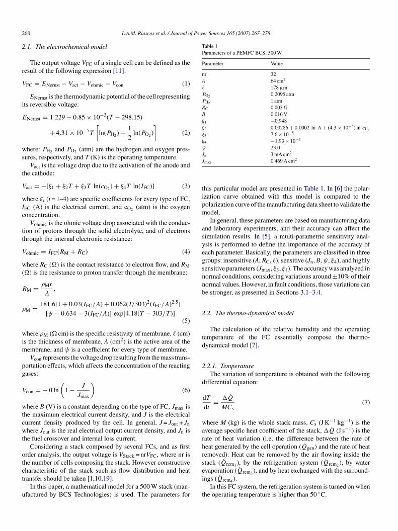
Fig. 2. Variation of output HR vs. input HR.

eaction. In general, the maximum efficiency occurs at about0% of fuel utilization (H2) and 50% of oxygen utilization.herefore, for a good concentration of O2 in the air through

he entire FC, λ should be bigger than 2 [11].To prevent the membrane from drying, some researchers (e.g.

11]) have proposed extra humidification on the input air. How-ver, the variation in the HR of the input air produces a very smalldjustment in the output HR; for example, a variation of 10%n the input HR represents a variation of approximately 2% onhe output HR. Thus, in many cases, the extra humidification ofhe input air is not enough to resolve the drying problem. Fig. 2llustrates the variation produced on the HR of output air by thedjustment in the HR of input air.

.3. Normal operation of a fuel cell

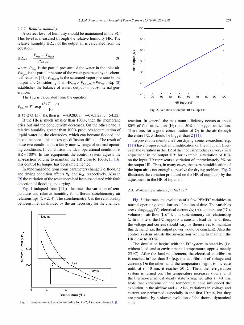
Fig. 3 illustrates the evolution of a few PEMFC variables inormal operating conditions as a function of time. The variablesre: voltagestack (V), electrical current IFC (A), temperature (◦C),olume of air flow (L s−1), and stoichiometry air relationship. In this test, the FC supports a constant-load demand; thus,

he voltage and current should vary by themselves to maintainhis demand (i.e. the output power would be constant). Also theontrol system adjusts the air-reaction volume to maintain theR close to 100%.The simulation begins with the FC system in stand-by (i.e.

ithout load, and at environmental temperature, approximately5 ◦C). After the load requirement, the electrical equilibriums reached in less than 3 s (e.g. the equilibrium of voltage andurrent). On the other hand, the temperature begins to increasentil, at t = 10 min, it reaches 50 ◦C. Then, the refrigerationystem is turned on. The temperature increases slowly untilhe thermo-dynamical steady state is reached after t = 40 min.ote that variations on the temperature have influenced the

volution in the airflow and λ. Also, variations in voltage andurrent are performed, especially in the first 10 min, but theyre produced by a slower evolution of the thermo-dynamicaltate.

270 L.A.M. Riascos et al. / Journal of Power Sources 165 (2007) 267–278

itions

3

•

•

lo

(gsmc

3

pcn

iswT

egmoo

R

wdoic

itdn(t

c

wmw

Fig. 3. Evolution of variables of a FC in normal cond

. Faults in fuel cells

In general, two types of fault detection can be considered:

Faults that can be detected by monitoring a specific variable.For example, the leak of fuel can be detected by installing aspecific gas sensor. In this case, a diagnosis is not necessary.Faults that cannot be detected directly by monitoring or faultsthat need some type of diagnosis.

Usually, fault detection on commercial fuel cell equipment isimited to detection of faults of the first type. This work focusesn fault detection of the second type.

Four types of faults in PEMFCs are considered in this study:1) fault in the air fan, (2) fault in the refrigeration system, (3)rowth of the fuel crossover, and (4) fault in the hydrogen pres-ure. The effects of these faults are included in the mathematicalodel to analyze the behavior of the FC system in fault operation

onditions.

.1. Fault in the air reaction fan

A reduction of the reaction air by a fault in the air fan canroduce two major effects: (1) accumulation of liquid water thanannot be evaporated and (2) reduction of O2 volume below thatecessary for a complete reaction with the H2.

A common method for removing excess water inside the FC

s using the air flowing through it. The correct variation of thetoichiometry λ maintains the HR proximal to 100%. However,hen a fault in the air fan takes place, this becomes impossible.his fault reduces the air reaction flow, which reduces the water

iIw

deriving from a mathematical model in MATLAB®.

vaporation volume and permits the accumulation of water. Areat accumulation of water causes the flooding of electrodesaking gas diffusion difficult and affecting the performance

f the FC. These effects are simulated by Eq. (9), which wasbtained empirically.

c(k) = Rc(0) ·(wacum(k)

const1

)0.8

, Jmax(k) = Jmax(0)

(wacum(k)/const1)1.2

(9)

here Jmax(0) is the value of the maximum electrical currentensity at the initial state (normal condition), Rc(0) is the valuef the variable at the initial state (normal condition), wacum(k)s the volume of water accumulated at instant k, and const1 is aonstant defining when the electrodes are led to flooding.

The second effect of a fault in the air fan occurs when λs below the practical and recommended value. In this case,he O2 concentration is reduced and the exit air completelyepleted of O2. This reduction of O2 concentration produces aegative effect on the ENernst (Eq. (2)) and increase on the VactEq. (3)). In this case, the O2 concentration changes accordingo empirical Eq. (10):

O2(k) = cO2(0)√const2/λ(k)

(10)

here cO2(k) is the O2 concentration at instant k, cO2(0) is the nor-al O2 concentration in the air, and const2 is a constant defininghen λ is lower than necessary for the chemical reaction.

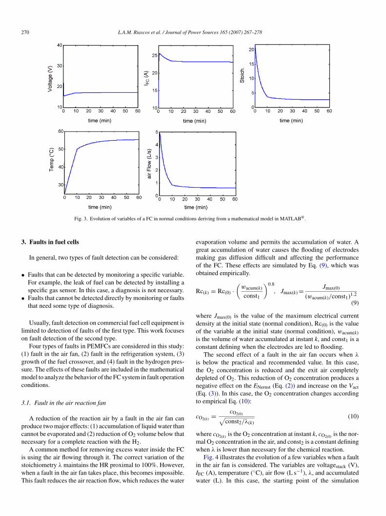
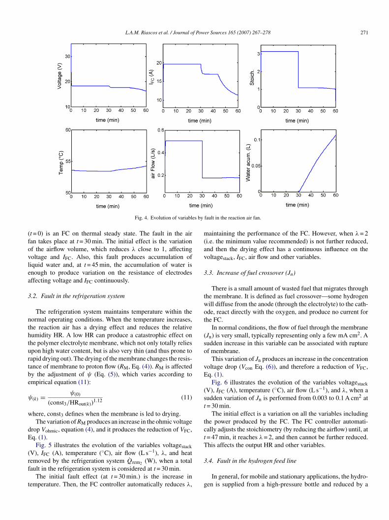
Fig. 4 illustrates the evolution of a few variables when a fault

n the air fan is considered. The variables are voltagestack (V),FC (A), temperature (◦C), air flow (L s−1), λ, and accumulatedater (L). In this case, the starting point of the simulation

L.A.M. Riascos et al. / Journal of Power Sources 165 (2007) 267–278 271

s by

(fovlea

3

nthturtbe

ψ

w

dE

(rf

t

m(av

3

twot

(so

vE

(st

tctT

Fig. 4. Evolution of variable

t = 0) is an FC on thermal steady state. The fault in the airan takes place at t = 30 min. The initial effect is the variationf the airflow volume, which reduces λ close to 1, affectingoltage and IFC. Also, this fault produces accumulation ofiquid water and, at t = 45 min, the accumulation of water isnough to produce variation on the resistance of electrodesffecting voltage and IFC continuously.

.2. Fault in the refrigeration system

The refrigeration system maintains temperature within theormal operating conditions. When the temperature increases,he reaction air has a drying effect and reduces the relativeumidity HR. A low HR can produce a catastrophic effect onhe polymer electrolyte membrane, which not only totally reliespon high water content, but is also very thin (and thus prone toapid drying out). The drying of the membrane changes the resis-ance of membrane to proton flow (RM, Eq. (4)). RM is affectedy the adjustment of ψ (Eq. (5)), which varies according tompirical equation (11):

(k) = ψ(0)

(const3/HRout(k))1.12 (11)

here, const3 defines when the membrane is led to drying.The variation of RM produces an increase in the ohmic voltage

rop Vohmic, equation (4), and it produces the reduction of VFC,q. (1).

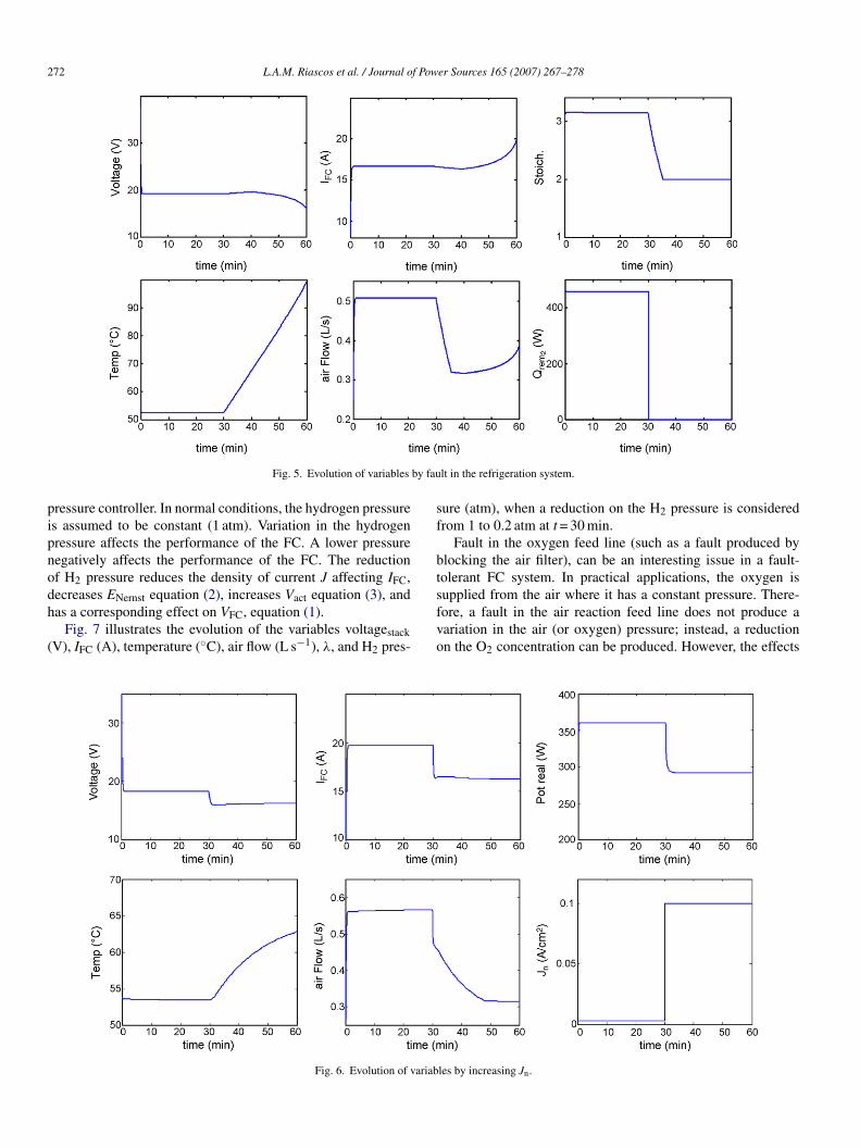
Fig. 5 illustrates the evolution of the variables voltagestackV), IFC (A), temperature (◦C), air flow (L s−1), λ, and heat

emoved by the refrigeration system Qrem2 (W), when a totalault in the refrigeration system is considered at t = 30 min.

The initial fault effect (at t = 30 min.) is the increase inemperature. Then, the FC controller automatically reduces λ,

3

g

fault in the reaction air fan.

aintaining the performance of the FC. However, when λ= 2i.e. the minimum value recommended) is not further reduced,nd then the drying effect has a continuous influence on theoltagestack, IFC, air flow and other variables.

.3. Increase of fuel crossover (Jn)

There is a small amount of wasted fuel that migrates throughhe membrane. It is defined as fuel crossover—some hydrogenill diffuse from the anode (through the electrolyte) to the cath-de, react directly with the oxygen, and produce no current forhe FC.

In normal conditions, the flow of fuel through the membraneJn) is very small, typically representing only a few mA cm2. Audden increase in this variable can be associated with rupturef membrane.

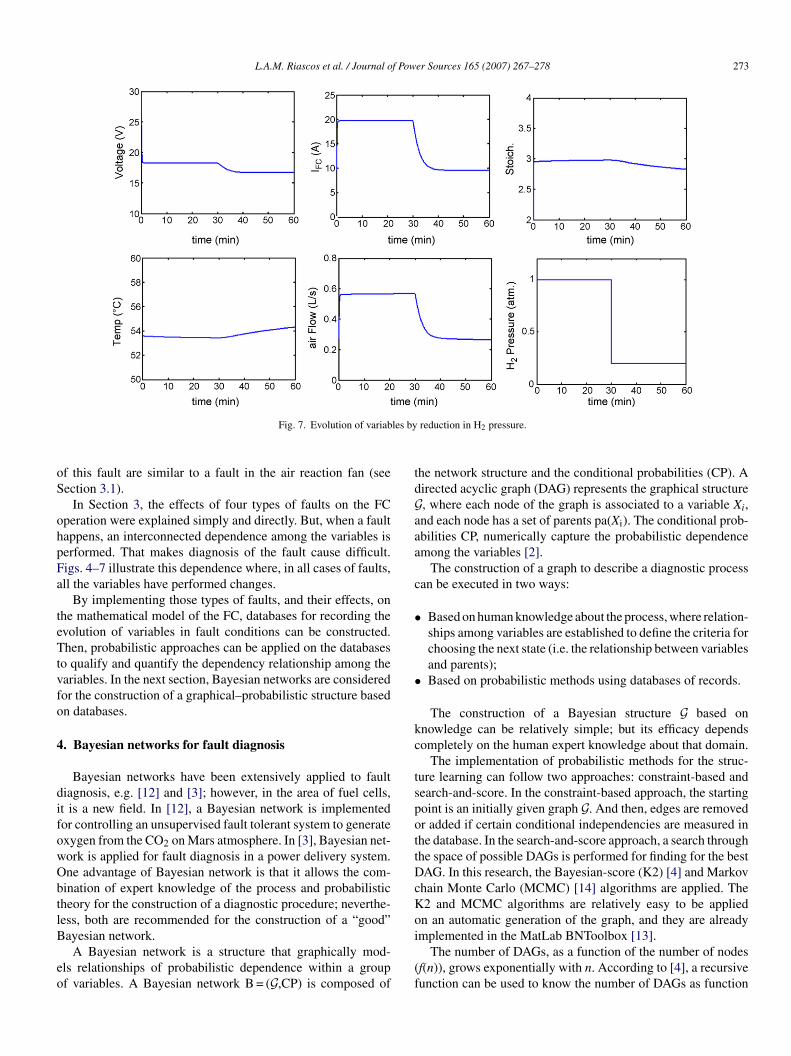
This variation of Jn produces an increase in the concentrationoltage drop (Vcon Eq. (6)), and therefore a reduction of VFC,q. (1).

Fig. 6 illustrates the evolution of the variables voltagestackV), IFC (A), temperature (◦C), air flow (L s−1), and λ, when audden variation of Jn is performed from 0.003 to 0.1 A cm2 at= 30 min.

The initial effect is a variation on all the variables includinghe power produced by the FC. The FC controller automati-ally adjusts the stoichiometry (by reducing the airflow) until, at= 47 min, it reaches λ= 2, and then cannot be further reduced.his affects the output HR and other variables.

.4. Fault in the hydrogen feed line

In general, for mobile and stationary applications, the hydro-en is supplied from a high-pressure bottle and reduced by a

272 L.A.M. Riascos et al. / Journal of Power Sources 165 (2007) 267–278

by fau

pipnodh

(

sf

bt

Fig. 5. Evolution of variables

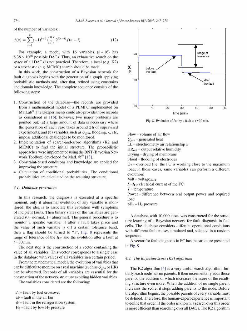
ressure controller. In normal conditions, the hydrogen pressures assumed to be constant (1 atm). Variation in the hydrogenressure affects the performance of the FC. A lower pressureegatively affects the performance of the FC. The reductionf H2 pressure reduces the density of current J affecting IFC,

ecreases ENernst equation (2), increases Vact equation (3), andas a corresponding effect on VFC, equation (1).

Fig. 7 illustrates the evolution of the variables voltagestackV), IFC (A), temperature (◦C), air flow (L s−1), λ, and H2 pres-

sfvo

Fig. 6. Evolution of variab

lt in the refrigeration system.

ure (atm), when a reduction on the H2 pressure is consideredrom 1 to 0.2 atm at t = 30 min.

Fault in the oxygen feed line (such as a fault produced bylocking the air filter), can be an interesting issue in a fault-olerant FC system. In practical applications, the oxygen is

upplied from the air where it has a constant pressure. There-ore, a fault in the air reaction feed line does not produce aariation in the air (or oxygen) pressure; instead, a reductionn the O2 concentration can be produced. However, the effects

les by increasing Jn.

L.A.M. Riascos et al. / Journal of Power Sources 165 (2007) 267–278 273

les by

oS

ohpFa

teTtvfo

4

difowObtlB

eo

tdGaaa

c

•

•

kc

tspottDcKo

Fig. 7. Evolution of variab

f this fault are similar to a fault in the air reaction fan (seeection 3.1).

In Section 3, the effects of four types of faults on the FCperation were explained simply and directly. But, when a faultappens, an interconnected dependence among the variables iserformed. That makes diagnosis of the fault cause difficult.igs. 4–7 illustrate this dependence where, in all cases of faults,ll the variables have performed changes.

By implementing those types of faults, and their effects, onhe mathematical model of the FC, databases for recording thevolution of variables in fault conditions can be constructed.hen, probabilistic approaches can be applied on the databases

o qualify and quantify the dependency relationship among theariables. In the next section, Bayesian networks are consideredor the construction of a graphical–probabilistic structure basedn databases.

. Bayesian networks for fault diagnosis

Bayesian networks have been extensively applied to faultiagnosis, e.g. [12] and [3]; however, in the area of fuel cells,t is a new field. In [12], a Bayesian network is implementedor controlling an unsupervised fault tolerant system to generatexygen from the CO2 on Mars atmosphere. In [3], Bayesian net-ork is applied for fault diagnosis in a power delivery system.ne advantage of Bayesian network is that it allows the com-ination of expert knowledge of the process and probabilisticheory for the construction of a diagnostic procedure; neverthe-ess, both are recommended for the construction of a “good”

ayesian network.

A Bayesian network is a structure that graphically mod-ls relationships of probabilistic dependence within a groupf variables. A Bayesian network B = (G,CP) is composed of

i

(f

reduction in H2 pressure.

he network structure and the conditional probabilities (CP). Airected acyclic graph (DAG) represents the graphical structure, where each node of the graph is associated to a variable Xi,nd each node has a set of parents pa(Xi). The conditional prob-bilities CP, numerically capture the probabilistic dependencemong the variables [2].

The construction of a graph to describe a diagnostic processan be executed in two ways:

Based on human knowledge about the process, where relation-ships among variables are established to define the criteria forchoosing the next state (i.e. the relationship between variablesand parents);Based on probabilistic methods using databases of records.

The construction of a Bayesian structure G based onnowledge can be relatively simple; but its efficacy dependsompletely on the human expert knowledge about that domain.

The implementation of probabilistic methods for the struc-ure learning can follow two approaches: constraint-based andearch-and-score. In the constraint-based approach, the startingoint is an initially given graph G. And then, edges are removedr added if certain conditional independencies are measured inhe database. In the search-and-score approach, a search throughhe space of possible DAGs is performed for finding for the bestAG. In this research, the Bayesian-score (K2) [4] and Markovhain Monte Carlo (MCMC) [14] algorithms are applied. The2 and MCMC algorithms are relatively easy to be appliedn an automatic generation of the graph, and they are already

mplemented in the MatLab BNToolbox [13].

The number of DAGs, as a function of the number of nodesf(n)), grows exponentially with n. According to [4], a recursiveunction can be used to know the number of DAGs as function

2 f Power Sources 165 (2007) 267–278

o

f

8so

fpaf

1

2

3

4

4

mioemttrt

vi

ccc

tcws

i

4

tpii

74 L.A.M. Riascos et al. / Journal o

f the number of variables:

(n) =n∑i=1

(−1)i+1(ni

)2i(n−i)f (n− i) (12)

For example, a model with 16 variables (n = 16) has.38 × 1046 possible DAGs. Thus, an exhaustive search on thepace of all DAGs is not practical. Therefore, a local (e.g. K2)r a stochastic (e.g. MCMC) search should be made.

In this work, the construction of a Bayesian network forault diagnosis begins with the generation of a graph applyingrobabilistic methods and, after that, refined using constrainsnd domain knowledge. The complete sequence consists of theollowing steps:

. Construction of the database—the records are providedfrom a mathematical model of a PEMFC implemented onMatLab®. Field experiments could also provide those recordsas considered in [16]; however, two major problems arepointed out: (a) a large amount of data is necessary wherethe generation of each case takes around 2 h of supervisedexperiments, and (b) variables such as Qgen, flooding, λ, etc,impose additional challenges to be monitored.

. Implementation of search-and-score algorithms (K2 andMCMC) to find the initial structure. The probabilisticapproaches were implemented using the BNT (Bayesian Net-work Toolbox) developed for MatLab® [13].

. Constraint-based conditions and knowledge are applied forimproving the structure.

. Calculation of conditional probabilities. The conditionalprobabilities are calculated on the resulting structure.

.1. Database generation

In this research, the diagnosis is executed at a specificoment, only if abnormal evolution of any variable is mon-

tored; the idea is to associate this evolution with symptomsf incipient faults. Then binary states of the variables are gen-rated (0 = normal, 1 = abnormal). The general procedure is toonitor a specific variable; if after a fault takes place and

he value of such variable is off a certain tolerance band,hen a flag should be turned to “1”. Fig. 8 represents theange of tolerance of the IFC and the evolution after a fault at= 30 min.

The next step is the construction of a vector containing thealue of all variables. This vector corresponds to a single casen the database with values of all variables in a certain period.

From the mathematical model, the evolution of variables thatan be difficult to monitor on a real machine (such as Qgen or HR)an be observed. Records of all variables are essential for theonstruction of the network structure avoiding hidden variables.

The variables considered are the following:

Jn = fault by fuel crossoveraF = fault in the air fanrF = fault in the refrigeration systemH2 = fault by low H2 pressure

tbti

Fig. 8. Evolution of IFC by a fault at t = 30 min.

Flow = volume of air flowQgen = generated heatLL = stoichiometry air relationship λHRout = output relative humidityDrying = drying of membraneFlood = flooding of electrodesOv = overload (i.e. the FC is working close to the maximumload; in those cases, same variables can perform a differentevolution)Volt = voltagestackI = IFC electrical current of the FCT = temperaturePower = difference between real output power and requiredloadpH2 = H2 pressure

A database with 10,000 cases was constructed for the struc-ure learning of a Bayesian network for fault diagnosis in fuelells. The database considers different operational conditionsith different fault causes simulated and, selected in a random

equence.A vector for fault diagnosis in FC has the structure presented

n Fig. 9.

.2. The Bayesian-score (K2) algorithm

The K2 algorithm [4] is a very useful search algorithm. Ini-ially, each node has no parents. It then incrementally adds thosearents, the addition of which increases the score of the result-ng structure even more. When the addition of no single parentncreases the score, it stops adding parents to the node. Before

he algorithm begins, the possible parents of every variable muste defined. Therefore, the human-expert experience is importanto define that order. If the order is known, a search over this orders more efficient than searching over all DAGs. The K2 algorithm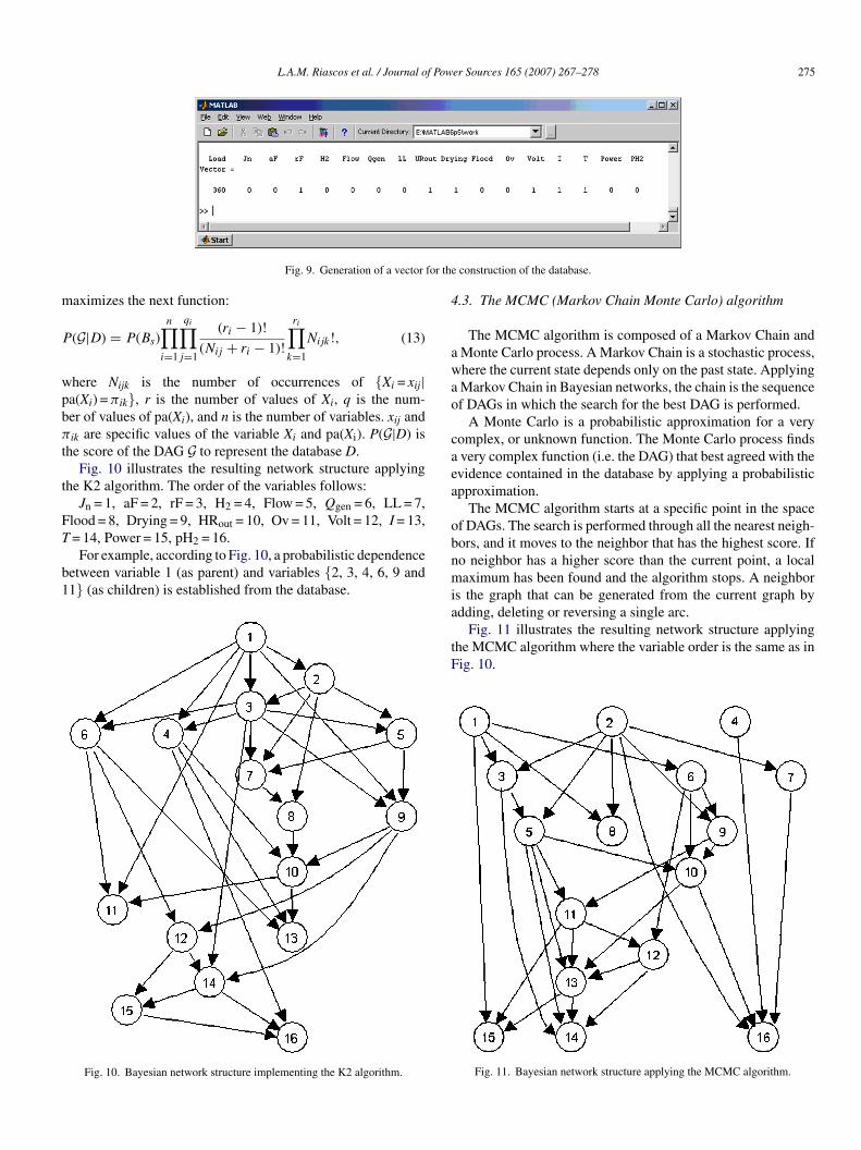

L.A.M. Riascos et al. / Journal of Power Sources 165 (2007) 267–278 275

for the

m

P

wpbπ

t

t

FT

b1

4

awao

caea

o

Fig. 9. Generation of a vector

aximizes the next function:

(G|D) = P(Bs)n∏i=1

qi∏j=1

(ri − 1)!

(Nij + ri − 1)!

ri∏k=1

Nijk!, (13)

here Nijk is the number of occurrences of {Xi = xij|a(Xi) =πik}, r is the number of values of Xi, q is the num-er of values of pa(Xi), and n is the number of variables. xij andik are specific values of the variable Xi and pa(Xi). P(G|D) is

he score of the DAG G to represent the database D.Fig. 10 illustrates the resulting network structure applying

he K2 algorithm. The order of the variables follows:Jn = 1, aF = 2, rF = 3, H2 = 4, Flow = 5, Qgen = 6, LL = 7,

lood = 8, Drying = 9, HRout = 10, Ov = 11, Volt = 12, I = 13,

= 14, Power = 15, pH2 = 16.For example, according to Fig. 10, a probabilistic dependence

etween variable 1 (as parent) and variables {2, 3, 4, 6, 9 and1} (as children) is established from the database.

Fig. 10. Bayesian network structure implementing the K2 algorithm.

bnmia

tF

construction of the database.

.3. The MCMC (Markov Chain Monte Carlo) algorithm

The MCMC algorithm is composed of a Markov Chain andMonte Carlo process. A Markov Chain is a stochastic process,here the current state depends only on the past state. ApplyingMarkov Chain in Bayesian networks, the chain is the sequencef DAGs in which the search for the best DAG is performed.

A Monte Carlo is a probabilistic approximation for a veryomplex, or unknown function. The Monte Carlo process findsvery complex function (i.e. the DAG) that best agreed with thevidence contained in the database by applying a probabilisticpproximation.

The MCMC algorithm starts at a specific point in the spacef DAGs. The search is performed through all the nearest neigh-ors, and it moves to the neighbor that has the highest score. Ifo neighbor has a higher score than the current point, a localaximum has been found and the algorithm stops. A neighbor

s the graph that can be generated from the current graph bydding, deleting or reversing a single arc.

Fig. 11 illustrates the resulting network structure applyinghe MCMC algorithm where the variable order is the same as inig. 10.

Fig. 11. Bayesian network structure applying the MCMC algorithm.

2 f Power Sources 165 (2007) 267–278

4

aMsbte

•••

caa

ataa(S(twap

dt(b

miebsptla

4

obc

lit

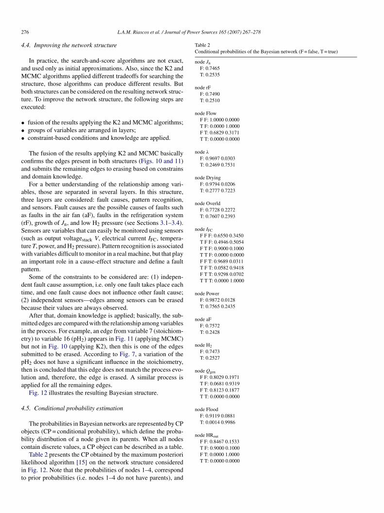
Table 2Conditional probabilities of the Bayesian network (F = false, T = true)

node Jn

F: 0.7465T: 0.2535

node rFF: 0.7490T: 0.2510

node FlowF F: 1.0000 0.0000T F: 0.0000 1.0000F T: 0.6829 0.3171T T: 0.0000 0.0000

node λF: 0.9697 0.0303T: 0.2469 0.7531

node DryingF: 0.9794 0.0206T: 0.2777 0.7223

node OverldF: 0.7728 0.2272T: 0.7607 0.2393

node IFC

F F F: 0.6550 0.3450T F F: 0.4946 0.5054F T F: 0.9000 0.1000T T F: 0.0000 0.0000F F T: 0.9689 0.0311T F T: 0.0582 0.9418F T T: 0.9298 0.0702T T T: 0.0000 1.0000

node PowerF: 0.9872 0.0128T: 0.7565 0.2435

node aFF: 0.7572T: 0.2428

node H2

F: 0.7473T: 0.2527

node Qgen

F F: 0.8029 0.1971T F: 0.0681 0.9319F T: 0.8123 0.1877T T: 0.0000 0.0000

node FloodF: 0.9119 0.0881T: 0.0014 0.9986

node HRout

F F: 0.8467 0.1533T F: 0.9000 0.1000

76 L.A.M. Riascos et al. / Journal o

.4. Improving the network structure

In practice, the search-and-score algorithms are not exact,nd used only as initial approximations. Also, since the K2 andCMC algorithms applied different tradeoffs for searching the

tructure, those algorithms can produce different results. Butoth structures can be considered on the resulting network struc-ure. To improve the network structure, the following steps arexecuted:

fusion of the results applying the K2 and MCMC algorithms;groups of variables are arranged in layers;constraint-based conditions and knowledge are applied.

The fusion of the results applying K2 and MCMC basicallyonfirms the edges present in both structures (Figs. 10 and 11)nd submits the remaining edges to erasing based on constrainsnd domain knowledge.

For a better understanding of the relationship among vari-bles, those are separated in several layers. In this structure,hree layers are considered: fault causes, pattern recognition,nd sensors. Fault causes are the possible causes of faults suchs faults in the air fan (aF), faults in the refrigeration systemrF), growth of Jn, and low H2 pressure (see Sections 3.1–3.4).ensors are variables that can easily be monitored using sensorssuch as output voltagestack V, electrical current IFC, tempera-ure T, power, and H2 pressure). Pattern recognition is associatedith variables difficult to monitor in a real machine, but that play

n important role in a cause-effect structure and define a faultattern.

Some of the constraints to be considered are: (1) indepen-ent fault cause assumption, i.e. only one fault takes place eachime, and one fault cause does not influence other fault cause;2) independent sensors—edges among sensors can be erasedecause their values are always observed.

After that, domain knowledge is applied; basically, the sub-itted edges are compared with the relationship among variables

n the process. For example, an edge from variable 7 (stoichiom-try) to variable 16 (pH2) appears in Fig. 11 (applying MCMC)ut not in Fig. 10 (applying K2), then this is one of the edgesubmitted to be erased. According to Fig. 7, a variation of theH2 does not have a significant influence in the stoichiometry,hen is concluded that this edge does not match the process evo-ution and, therefore, the edge is erased. A similar process ispplied for all the remaining edges.

Fig. 12 illustrates the resulting Bayesian structure.

.5. Conditional probability estimation

The probabilities in Bayesian networks are represented by CPbjects (CP = conditional probability), which define the proba-ility distribution of a node given its parents. When all nodesontain discrete values, a CP object can be described as a table.

Table 2 presents the CP obtained by the maximum posterioriikelihood algorithm [15] on the network structure consideredn Fig. 12. Note that the probabilities of nodes 1–4, correspondo prior probabilities (i.e. nodes 1–4 do not have parents), and

F T: 0.0000 1.0000T T: 0.0000 0.0000

L.A.M. Riascos et al. / Journal of Power Sources 165 (2007) 267–278 277

Table 2 (Continued )

node VoltF: 0.9637 0.0363T: 0.8113 0.1887

node TF: 1.0000 0.0000T: 0.7604 0.2396

node pH2

tp

Gdciao

ebvoSFidIdscIamH

oi

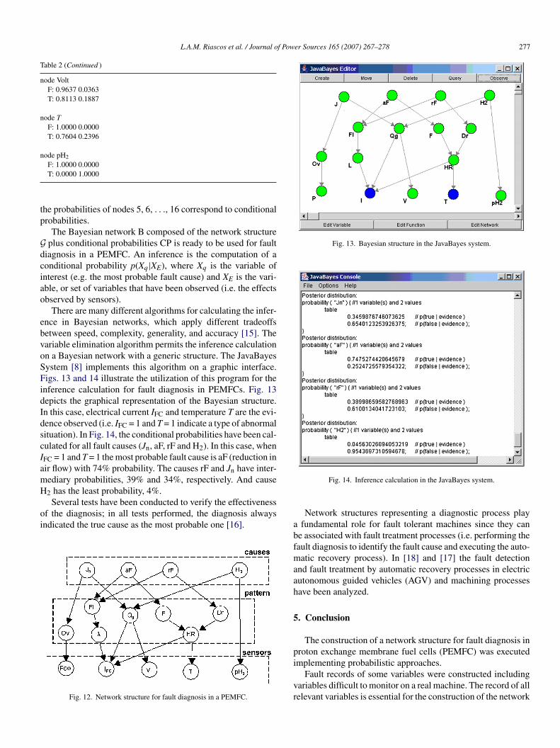
Fig. 13. Bayesian structure in the JavaBayes system.

F: 1.0000 0.0000T: 0.0000 1.0000

he probabilities of nodes 5, 6, . . ., 16 correspond to conditionalrobabilities.

The Bayesian network B composed of the network structureplus conditional probabilities CP is ready to be used for fault

iagnosis in a PEMFC. An inference is the computation of aonditional probability p(Xq|XE), where Xq is the variable ofnterest (e.g. the most probable fault cause) and XE is the vari-ble, or set of variables that have been observed (i.e. the effectsbserved by sensors).

There are many different algorithms for calculating the infer-nce in Bayesian networks, which apply different tradeoffsetween speed, complexity, generality, and accuracy [15]. Theariable elimination algorithm permits the inference calculationn a Bayesian network with a generic structure. The JavaBayesystem [8] implements this algorithm on a graphic interface.igs. 13 and 14 illustrate the utilization of this program for the

nference calculation for fault diagnosis in PEMFCs. Fig. 13epicts the graphical representation of the Bayesian structure.n this case, electrical current IFC and temperature T are the evi-ence observed (i.e. IFC = 1 and T = 1 indicate a type of abnormalituation). In Fig. 14, the conditional probabilities have been cal-ulated for all fault causes (Jn, aF, rF and H2). In this case, whenFC = 1 and T = 1 the most probable fault cause is aF (reduction inir flow) with 74% probability. The causes rF and Jn have inter-ediary probabilities, 39% and 34%, respectively. And cause2 has the least probability, 4%.

Several tests have been conducted to verify the effectiveness

f the diagnosis; in all tests performed, the diagnosis alwaysndicated the true cause as the most probable one [16].

Fig. 12. Network structure for fault diagnosis in a PEMFC.

abfmaah

5

pi

vr

Fig. 14. Inference calculation in the JavaBayes system.

Network structures representing a diagnostic process playfundamental role for fault tolerant machines since they can

e associated with fault treatment processes (i.e. performing theault diagnosis to identify the fault cause and executing the auto-atic recovery process). In [18] and [17] the fault detection

nd fault treatment by automatic recovery processes in electricutonomous guided vehicles (AGV) and machining processesave been analyzed.

. Conclusion

The construction of a network structure for fault diagnosis inroton exchange membrane fuel cells (PEMFC) was executed

mplementing probabilistic approaches.

Fault records of some variables were constructed includingariables difficult to monitor on a real machine. The record of allelevant variables is essential for the construction of the network

2 f Pow

sl

mM“ipe

tbmd

aon

taa

A

cP

R

[

[

[

[[

[

[

[

[faults in automated machines based on Petri nets and Bayesian networks,in: Proceedings of IEEE-ISIE (International Symposium in Industrial Elec-tronics), Rio de Janeiro, Brazil, 2003.

[19] M. Santis, S.A. Freunberger, M. Papra, A. Wokaun, F.N. Buchi, J. Power

78 L.A.M. Riascos et al. / Journal o

tructure avoiding hidden variables, especially on intermediaryayers.

For the construction of a network structure, the sole imple-entation of probabilistic approaches (such as the K2 andCMC algorithms), is not enough for the construction of a

good” network, as presented in Figs. 10 and 11. An understand-ng of the process (e.g. processes in PEMFCs), is recommended,articularly for applying constrain-based conditions and knowl-dge to improve the network structure.

For the diagnostic process (i.e. the inference calculation),he evidence was based on observations of variables that cane easily monitored by sensors like voltmeters, ammeters, ther-ocouples, etc. This allows an easy implementation of fault

iagnostic processes in FC systems.The tests have shown agreement between the inference results

nd the original fault causes. They will allow the implementationf an on-line supervisor for fault diagnosis applying Bayesianetworks constructed as described in this research.

Topics such as the study of fault effects in FCs, the construc-ion of network structures for fault diagnosis in FCs, and theirssociation to fault treatment processes are still under study, andre still open to research contributions.

cknowledgment

The authors thank FAPESP, CNPq, and CAPES for the finan-ial support to the present project, and Prof. J.M. Correa androf. F.G. Cozman for academic contribution.

eferences

[1] P.A.C. Chang, J. St-Pierre, J. Stumper, B. Wetton, J. Power Sources 162(1) (2006) 340–355.

er Sources 165 (2007) 267–278

[2] D.M. Chickering, J. Mach. Learn. Res. 3 (2002) 507–554.[3] C.F. Chien, S.L. Chen, Y.S. Lin, IEEE Trans. Power Deliv. 17 (3) (2002)

785–793.[4] G.F. Cooper, E. Herskovits, Mach. Learn. 9 (1992) 309–347.[5] J.M. Correa, F.A. Farret, L.N. Canha, M.G. Simoes, V.A. Popov, IEEE

Trans. Energy Conver. 20 (1) (2005) 211–218.[6] J.M. Correa, F.A. Farret, L.N. Canha, M.G. Simoes, IEEE Trans. Ind.

Electron. 51 (5) (2004) 1103–1112.[7] J.M. Correa, F.A. Farret, J.R. Gomes, M.G. Simoes, IEEE Trans. Ind. Appl.

Soc. 39 (4) (2003) 1136–1142.[8] F.G. Cozman, http://www-2.cs.cmu.edu/∼javabayes/ (2001).[9] N. Fouquet, C. Doulet, C. Nouillant, G. Dauphin-Tanguy, B. Ould Boua-

mama, J. Power Sources 159 (2) (2006) 905–913.10] S.A. Freunberger, M. Santis, I.A. Schneider, A. Wokaun, F.N. Buchi, J.

Electrochem. Soc. 153 (2) (2006), A396–A405 & A909–A913.11] J. Larminie, A. Dicks, Fuel Cell Systems Explained, John Wiley & Sons

Ltd., 2003.12] U. Lerner, B. Moses, M. Scott, S. McIlraith, D. Koller, Proceedings of 18th

Conference on Uncertainty in AI, 2002, pp. 301–310.13] K. Murphy, (2005). http://bnt.sourceforge.net/.14] J. Pearl, Causality: Models Reasoning and Inference, Cambridge University

Press, 2000.15] J. Pearl, Probabilistic Reasoning in Intelligent Systems: Networks of Plau-

sible Inference, Morgan Kaufmann Publ., 1988.16] L.A.M. Riascos, M.G. Simoes, F.G. Cozman, P.E. Miyagi, Proceedings

of the 41st IEEE-IAS, Industry Application Society, Tampa-FL, USA,2006.

17] L.A.M. Riascos, P.E. Miyagi, Cont. Eng. Pract. 14 (2006) 397–408.

18] L.A.M. Riascos, F.G. Cozman, P.E. Miyagi, Detection and treatment of

Sources 161 (2) (2006) 1076–1083.