a bayesian approach to paired comparison rankings based on a graphical model

Computational Statistics & Data Analysis 48 (2005) 269–290www.elsevier.com/locate/csda

A Bayesian approach to paired comparisonrankings based on a graphical model

Hea-Jung Kim∗

Department of Statistics, Dongguk University, Pil-dong 3-Ga, Chung-Gu, Seoul 100-715,Republic of Korea

Received 1 August 2003; received in revised form 1 January 2004; accepted 13 January 2004

Abstract

A Bayesian method for 1nding an optimal ranking in scalar functions of K population pa-rameters is developed. This is based on the paired comparison experimental arrangement whoseresults can naturally be represented by a completely oriented graphical model. Introducing pos-terior preference probabilities satisfying a strong stochastic transitivity condition to the model,a criterion for the optimal ranking is suggested. Necessary theories involved in the method andsome computational aspects are provided. As illustrated examples, ranking in generalized vari-ances of K multivariate normal populations and in products of independent normal means aregiven.c© 2004 Elsevier B.V. All rights reserved.

Keywords: Graphical model; Hamiltonian path; Paired comparison ranking; Stochastic transitivity;Generalized variances

1. Introduction

Consider K independent populations with parameters �1; : : : ; �K , and suppose thatthere is an interest in the relative magnitudes of �k ’s. This is situation arising frequentlyin the paired comparison experimental arrangement. At this point various familiar meth-ods and theories are possible for solving the problem of the interest. A great deal ofwork has focused on the problem of multiple inferences and simultaneous con1denceintervals for �k ’s (Hsu, 1996; Bauer, 1997; Pennello, 1997 and references therein).Other work on the selection problem has developed and evaluated methods for picking

∗ Tel.: +82-2260-3221; fax: +82-2267-0998.E-mail address: [email protected] (H.-J. Kim).

0167-9473/$ - see front matter c© 2004 Elsevier B.V. All rights reserved.doi:10.1016/j.csda.2004.01.002

mailto:[email protected]

270 H.-J. Kim /Computational Statistics & Data Analysis 48 (2005) 269–290

the best population in terms of magnitude of �k ’s (Bechhofer et al., 1995; Kim andNelson, 2001 among others). Another works are about the probability distribution ofrankings (Gilbert, 2003 and references therein), and the others are paired comparisonranking in �k ’s (Davison and Solomon, 1973; David, 1987).

Unlike the previous works, of particular interest of this paper is the ranking of scalarfunctions of parameter vector or matrix, f(�k)’s, that may exhibit heterogeneity bothin the parameters, �k ’s, of interest and in the characteristic of the populations. Thepaired comparison ranking P = (p1; : : : ; pK) de1ned (in terms of preference order) asthe smallest numbers in the set {1; : : : ; K} such that pi ¡pj if f(�i) → f(�j) (readthis as f(�i) is preferred to f(�j)), for i; j=1; : : : ; K , is useful in describing magnitudeof competitors in the multiple comparisons. Variations on this basic theme are commonin many 1elds, including environmental applications, such as exposure assessment andrisk modeling (1nding ranks in several products of n normal means, Sun and Ye,1995), quality assessment in engineering (ranks in determinant of multivariate normalcovariance matrices, Rencher, 2002), and economics (global economic competition,Amanto and Amanto, 2001).

We present here a graphical approach to the analysis of data arising from pairedcomparison ranking. A graphical model is considered: A completely oriented graph(a graph which every pair of nodes is connected by a single uniquely directed edge;Skiena, 1990, p. 175) that incorporates preference probabilities obtained from a multiplepaired comparisons. The objectives of the approach are (i) to construct a graphicalmodel that bring unique ranking in the parameters, f(�k)’s, and the power of visualinterpretation to bear on the paired comparison ranking, and (ii) to provide a criterionfor ranking in the parameters, f(�k)’s, and show that it is especially appropriate whena strong stochastic transitivity condition can be imposed on the preference probabilities.

Section 2 presents a completely oriented graph that is closely related to the pairedcomparison ranking, which can be used to make an optimal ranking. In Section 3,incorporating a probability model to each node of the graph, we construct a graphicalmodel designed particularly for the paired comparison ranking in parameter functions ofseveral probability models. Several properties of the graphical model are also examined.We then suggest a criterion for obtaining an optimal paired comparison ranking in theparameter functions of interest. In Section 4, some computational aspects are discussed,and Sections 5 and 6 illustrate our method by using four examples. Finally, someconclusions are given in Section 7.

2. Relation to graph theory

A tournament is a digraph whose underlying graph is a completely directed graph.The directed graph is a natural way of representing the results of paired comparisonexperiments. The mathematical literature treats problem related to the experiments usingthe language of round robin tournaments (see Harary et al., 1965). For the tournamentswe can consider a 1nite oriented graph G(X; R) that consists of X say X ={1; 2; : : : ; K},of vertices and a collection of arcs R where arc is of form x → y with x and y in X .A rank order (simply ranking) is an arrangement P = (p1; p2; : : : ; pK) of the objects

H.-J. Kim /Computational Statistics & Data Analysis 48 (2005) 269–290 271

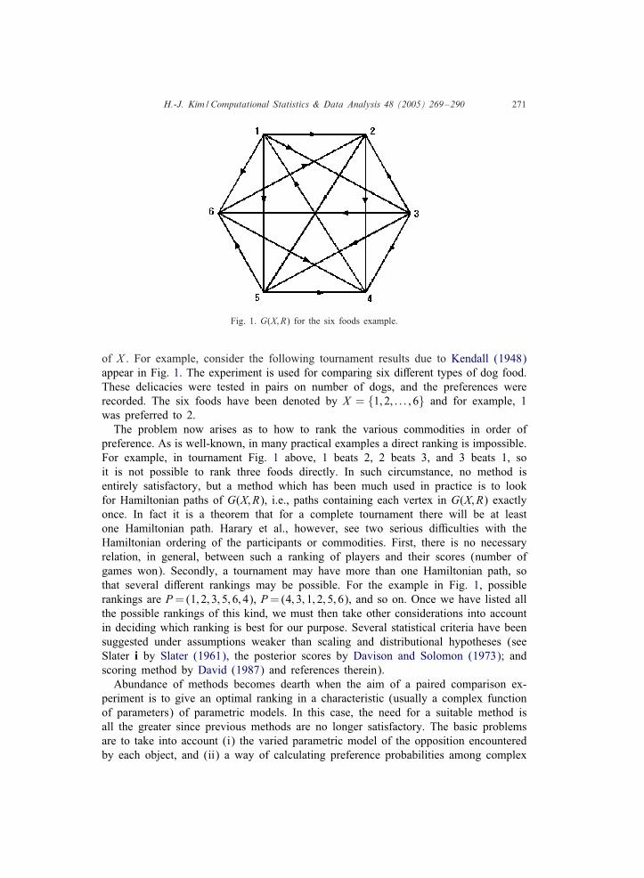
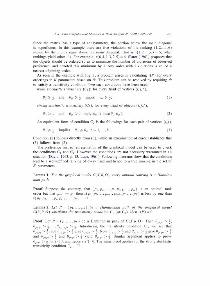
Fig. 1. G(X; R) for the six foods example.

of X . For example, consider the following tournament results due to Kendall (1948)appear in Fig. 1. The experiment is used for comparing six diJerent types of dog food.These delicacies were tested in pairs on number of dogs, and the preferences wererecorded. The six foods have been denoted by X = {1; 2; : : : ; 6} and for example, 1was preferred to 2.

The problem now arises as to how to rank the various commodities in order ofpreference. As is well-known, in many practical examples a direct ranking is impossible.For example, in tournament Fig. 1 above, 1 beats 2, 2 beats 3, and 3 beats 1, soit is not possible to rank three foods directly. In such circumstance, no method isentirely satisfactory, but a method which has been much used in practice is to lookfor Hamiltonian paths of G(X; R), i.e., paths containing each vertex in G(X; R) exactlyonce. In fact it is a theorem that for a complete tournament there will be at leastone Hamiltonian path. Harary et al., however, see two serious diKculties with theHamiltonian ordering of the participants or commodities. First, there is no necessaryrelation, in general, between such a ranking of players and their scores (number ofgames won). Secondly, a tournament may have more than one Hamiltonian path, sothat several diJerent rankings may be possible. For the example in Fig. 1, possiblerankings are P=(1; 2; 3; 5; 6; 4), P=(4; 3; 1; 2; 5; 6), and so on. Once we have listed allthe possible rankings of this kind, we must then take other considerations into accountin deciding which ranking is best for our purpose. Several statistical criteria have beensuggested under assumptions weaker than scaling and distributional hypotheses (seeSlater i by Slater (1961), the posterior scores by Davison and Solomon (1973); andscoring method by David (1987) and references therein).

Abundance of methods becomes dearth when the aim of a paired comparison ex-periment is to give an optimal ranking in a characteristic (usually a complex functionof parameters) of parametric models. In this case, the need for a suitable method isall the greater since previous methods are no longer satisfactory. The basic problemsare to take into account (i) the varied parametric model of the opposition encounteredby each object, and (ii) a way of calculating preference probabilities among complex


functions of parameters. Our method is obtained as a result of theoretical analysis of agraphical model where posterior preference probabilities among functions of parametersin the models are incorporated with the graph G(X; R). In outline, special features ofour method and results are as follows: (i) In each vertex of the graph G(X; R), weassume a parametric model to be compared. (ii) Our method is designed to obtain anoptimal paired comparison ranking in any functions of parameter vector (or matrix)of the hypothesized models. (iii) A simple criterion and procedure for obtaining theoptimal paired comparison ranking is given by utilizing a transitivity condition for thegraphical model. (iv) Under the condition, we show that there is unique Hamiltonianpath in the graphical model and its rank order is equivalent to the optimal pairedcomparison ranking.

3. The graphical model

Using the 1nite directed graph G(X; R), one can formulate a graphical model for thepaired comparisons. Suppose K parameters (scalar functions of �k ; f(�k)’s, k=1; : : : ; K)are to be compared in pairs with data being obtained from K populations. For this case,the oriented graph is de1ned by G(X; R), where X ={1; : : : ; K} is of a set of parameterindices called vertices and R = {(i; j)|i∈X; j ∈X; i �= j} is the set of arcs.

Suppose a K × K matrix � = {�ij} (i; j = 1; : : : ; K), where �ij = Pr(i → j) denotesthe probability of preference for ith function f(�i) over jth function f(�j), so that�ij + �ji = 1, and �ii = 1

2 . Then the graphical model for the paired comparisons is apair (G;�) where G is the oriented graph and � is the K × K preference probabilitymatrix. From now on we shall denote the graphical model by G(X; R;�).

Given the model G(X; R;�), one can obtain a rank order P of the parameters whereP = (p1; : : : ; pK) is de1ned (in terms of preference order) as the smallest numbers inthe set {1; : : : ; K} such that pi ¡pj if f(�pi) → f(�pj).

Let v(P) denote the number of violations of the observed preference, that is thenumber of arcs pi → pj in R such that pj precedes pi in P. The so-called preferencematrix representation of the graphical model is useful for determining v(P). For givenP, the preference matrix contains a plus in its i; jth place if �pipj ¿

12 (i.e. if pi → pj)

a minus if �pjpi ¿12 (i.e. if pj → pi) and a dot if �pipj = 1

2 . Suppose G(X; R;�) inFig. 1 has the preference probabilities �pipj =Pr(pi → pj)= 3

4 for all pi and pj. Thenthe rank P = (1; 2; : : : ; 6) obtained from Fig. 1 would yield the preference matrix:

· + + − + +

− · − + + −− + · + + +

+ − − · − −− − − + · +

− + − + − ·

:


Since the matrix has a type of antisymmetry, the portion below the main diagonalis superMuous. In this example there are 1ve violations of the ranking (1; 2; : : : ; 6)shown by the minus signs above the main diagonal. That is v(1; 2 : : : ; 6) = 5; otherrankings yield other v’s. For example, v(6; 4; 1; 3; 2; 5) = 6. Slater (1961) proposes thatthe objects should be ordered so as to minimize the number of violations of observedpreference, and denoted this minimum by i. Any order with i violations is called anearest adjoining order.

As seen in the example with Fig. 1, a problem arises in calculating v(P) for everyorderings in K parameters based on �. This problem can be resolved by requiring �to satisfy a transitivity condition. Two such conditions have been used:weak stochastic transitivity (C1): for every triad of vertices (i; j; ‘),

�ij¿ 12 and �j‘¿ 1

2 imply �i‘¿ 12 ; (1)

strong stochastic transitivity (C2): for every triad of objects (i; j; ‘),

�ij¿ 12 and �j‘¿ 1

2 imply �i‘¿max(�ij; �j‘): (2)

An equivalent form of condition C2 is the following: for each pair of vertices (i; j),

�ij¿ 12 implies �i‘¿ �j‘ ‘ = 1; : : : ; K: (3)

Condition (2) follows directly from (3), while an examination of cases establishes that(3) follows from (2).

The preference matrix representation of the graphical model can be used to checkthe conditions C1 and C2. However the conditions are not necessary warranted in allsituation (David, 1963, p. 13; Luce, 1961). Following theorems show that the conditionslead to a well-de1ned ranking of every triad and hence to a true ranking in the set ofK parameters.

Lemma 1. For the graphical model G(X; R;�), every optimal ranking is a Hamilto-nian path.

Proof. Suppose the contrary, that (p1; p2; : : : ; pi; pi+1; : : : ; pK) is an optimal rankorder but that pi+1 → pi, then v(p1; p2; : : : ; pi−1; pi+1; pi; : : : ; pK) is less by one thanv(p1; p2; : : : ; pi; pi+1; : : : ; pK).

Lemma 2. Let P = (p1; : : : ; pK) be a Hamiltonian path of the graphical modelG(X; R;�) satisfying the transitivity condition C1 (or C2), then v(P) = 0.

Proof. Let P = (p1; : : : ; pK) be a Hamiltonian path of G(X; R;�). Then �p1p2 ¿12 ,

�p2 ;p3 ¿12 ; : : : ; �pK−1pK ¿ 1

2 . Introducing the transitivity condition C1, we see that�p1p2 ¿

12 , and �p2 ;p3 ¿

12 give �p1p3 ¿

12 . Now �p1p3 ¿

12 and �p3p4 ¿

12 give �p1p4 ¿

12 ,

and �p1p4 ¿12 and �p4p5 ¿

12 yield �p1p5 ¿

12 . Similar argument applies to prove

�pipj ¿12 for i¡ j. and hence v(P)=0. The same proof applies for the strong stochastic

transitivity condition C2.


It is well known that, for a directed graph G(X; R) obtained from a complete pairedcomparisons, there exists at least one Hamiltonian path (cf. Harary et al., 1965). Thisfact and Lemma 2 imply that any graphical model G(X; R;�) satisfying C1 (or C2),has an optimal ranking P of K parameters achieving v(P) = 0. We shall call a pairedcomparison ranking P having v(P) = 0 is the ‘optimal paired comparison ranking’.

Theorem 1. If a graph model G(X; R;�), X = {1; : : : ; K}, satis9es the transitivitycondition C1 (or C2). Then there exists one and only one Hamiltonian path of Kvertices, P = (p1; : : : ; pK) yielding v(P) = 0.

Proof. Lemmas 1 and 2 note that a Hamiltonian path of G(X; R;�), X = {1; : : : ; K},yields the optimal paired comparison ranking P=(p1; : : : ; pK). Suppose there is anotherHamiltonian path yielding the optimal paired comparison ranking, say P∗=(p∗

1 ; : : : ; p∗K).

Then, under G(X; R;�) and the condition C1 (or C2), the two optimal rankings withv(P) = v(P∗) = 0 would yield �pipj ¿

12 and �p∗

i p∗j¿ 1

2 for all i¡ j; i; j = 1; : : : ; K .These probability relations can be satis1ed only if pi = p∗

i and pj = p∗j for all i¡ j,

i.e. P = P∗, because �pipj + �pjpi = 1 and �p∗i p

∗j

+ �p∗j p

∗i

= 1.

Theorem 2. When the strong stochastic transitivity condition C2 is satis9ed, theoptimal paired comparison ranking P = (p1; : : : ; pK) of a graphical model G(X; R;�)with X = {1; : : : ; K}, is equivalent to the ranking according to the row-sum scoresof �.

Proof. Without loss of generality, we assume that P = (1; 2; : : : ; K). The condition C2

of G(X; R;�) implies the following relations: It is straight forward to see, from (3),that �k‘¿ �k+1‘, for ‘¿k, k=1; : : : ; K−1; ‘=1; : : : ; K . For ‘=k, �k‘= 1

2 by de1nition.For ‘¡k, �‘k+1¿ �‘k by (2). This implies �k‘¿ �k+1‘, because �k‘ = 1 − �‘k and�k+1‘ = 1 − �‘k+1. Decomposing kth and k + 1th row-sum scores of �, we have

K∑‘=1

�k‘ =∑‘¡k

�k‘ + �kk +∑‘¿k

�k‘

andK∑

‘=1

�k+1‘ =∑‘¡k

�k+1‘ + �k+1k +∑‘¿k

�k+1‘;

respectively. Since �kk¿�k+1k for P = (1; 2; : : : ; K), we have∑K

‘=1 �k‘¿∑K

‘=1 �k+1‘,k = 1; : : : ; K − 1.

4. Bayesian computational aspects

The practical matter of determining the optimal paired comparison ranking is noteasy. A direct algorithm would be to enumerate all K! possible rankings in G(X; R;�),score v in each ranking based on �, and 1nd the optimal ranking P with minimum


score v. Alternatively, one may obtain all the Hamiltonian paths from a graphicalmodel G(X; R;�) with K vertices, and then score v in each path to 1nd the optimalranking. When a model G(X; R;�) satis1es the weak stochastic transitivity conditionC1, constructing the optimal paired comparison ranking of the parameters in the modelis equivalent to 1nding a Hamiltonian path of the model having v(P)=0 by Theorem 1.However, 1nding Hamiltonian paths in a graphical model is diKcult problem and thisproblem has not been resolved yet (see, Adelman, 1994; Fu et al., 2003).

However the optimal ranking can be easily obtained when the strong stochastictransitivity condition C2 is satis1ed in the paired comparison ranking of K parameters.Suppose that parameters of K populations, �1; : : : ; �K , are compared in all possibleK(K −1)=2 diJerent pairings. As seen in Theorem 2, the simplest procedure is to rankthem according to the vector w of row-sum scores (cf. David, 1987),

w = �1; (4)

where 1 is the column vector of K ones and � is the preference probability matrix.Suppose we have G(X; R;�) with a set of vertices X = {1; : : : ; K} where kth vertex

denotes a scalar function f(�k) of parameter �k of a probability model (or population)�k , k = 1; : : : ; K . If sample is available from each �k , then following theorem makesthe model G(X; R;�) satisfy C2.

Theorem 3. Suppose ranking is conducted according to descending order of magnitudein f(�k)’s. If �= {�ij} is obtained from a proper joint posterior distribution of �k ’ssuch that

�ij = pr(i → j) =pr(�iM ¿ 0|Data)

pr(�iM ¿ 0|Data) + pr(�jM ¿ 0|Data);

where i; j = 1; : : : ; K , �rM = f(�r) − fM ; r = i; j, and fM =∑K

k=1 f(�k)=K . ThenG(X; R;�) warrants the strong stochastic transitivity condition C2.

Proof. For each pair of vertices (i; j), �ij¿ 12 implies pr(�iM ¿ 0|Data)¿

pr(�iM ¿ 0|Data) which in turn implies �i‘¿ �j‘, ‘ = 1; : : : ; K , in that �ij is mono-tonic increasing in pr(�iM ¿ 0|Data). Thus, for any triad of vertices (i; j; ‘), if �ij¿ 1

2and �j‘¿ 1

2 then �i‘¿ �j‘ and �i‘¿ �ij, i.e. �i‘¿max(�ij; �j‘), the strong stochastictransitivity condition C2.

Sometimes ranking need to be conducted according to ascending order of magnitudein f(�k)’s. In this case, Theorem 3 can be modi1ed by de1ning �ij = Pr(�iM ¡0|Data)={Pr(�iM ¡ 0|Data) + Pr(�jM ¡ 0|Data)}. For positive f(�k)’s, if we de-1ne �ij = f(�i)=fM , Theorem 3 with �ij = Pr(�iM ¡ 1|Data)={Pr(�iM ¡ 1|Data) +Pr(�jM ¡ 1|Data)} and �ij = Pr(�iM ¿ 1|Data)={Pr(�iM ¿ 1|Data) + Pr(�jM ¿1|Data)} are also true for ascending order and descending order of magnitudes inf(�k)’s, respectively. This will be discussed in Section 5. In order to de1ne the pos-terior preference probabilities �ij’s, we use the posterior mean of f(�k)’s, fM , asa reference quantity. The other choices of the reference quantity can be used. For


example, fMed = Median{f(�1); : : : ; f(�K)} would better reMects the diJerence amongf(�k)’s in computing �ij.

5. Application of rankings in generalized variances

5.1. Graphical model

The generalized variance can be used to rank distinct groups and populations inorder of their dispersion or spread (see Grizzle and Allen, 1969; Press, 1982; Rencher,2002). For example, a certain product, such as semiconductor, produced by a number ofcompanies is characterized by a vector of p measurements. Although the same productis produced on the average, the companies can be distinguished on the basis of theirassociated generalized variances. The problem arises as to how to rank the variousgeneralized variances in order of their magnitude. The problem can be resolved by thepaired comparison ranking in the generalized variances, |"k |’s, of K populations. LetX = {1; 2; : : : ; K} be the set of vertices whose element correspond to index of |"k |denoting each population distribution and let element �ij of � denote the posteriorpreference probability that is

pr(i → j) =pr(|"i|¡ |"M‖data)

pr(|"i|¡ |"M‖data) + pr(|"j|¡ |"M‖data) ;

where |"M |=∑Kk=1 |"k |=K . Then G1(X; R;�) is a graphical model for the paired com-

parison ranking in K generalized variances and warrants the strong stochastic transitivitycondition for �.

Followings are need to calculate posterior preference probabilities for the pairedcomparison ranking in the K generalized variances.

5.2. The posterior distribution

Suppose X1(i); : : : ; XNi(i) are independent p-variate observations from ith population�i ∼ Np($i; %−1

i ), i = 1; : : : ; K , where %i = "−1i , the precision matrix. Let

QX (i) =Ni∑‘=1

X‘(i)=Ni; and Vi =Ni∑‘=1

(X‘(i) − QX (i))(X‘(i) − QX (i))′:

Then the joint p.d.f. of QX (i)’s and Vi’s is proportional toK∏i=1

|Vi|(Ni−p−2)=2|%i|Ni=2etr{

−12%i[Vi + Ni( QX (i) − $i)( QX (i) − $i)′]

}; (5)

where etr{A}=exp{trA}. To assure very little information is contributed to the analysisby a subjective prior density, we assume diJuse prior

p($i; %i; i = 1; : : : ; K) ˙K∏i=1

|%i|−(p+1)=2: (6)


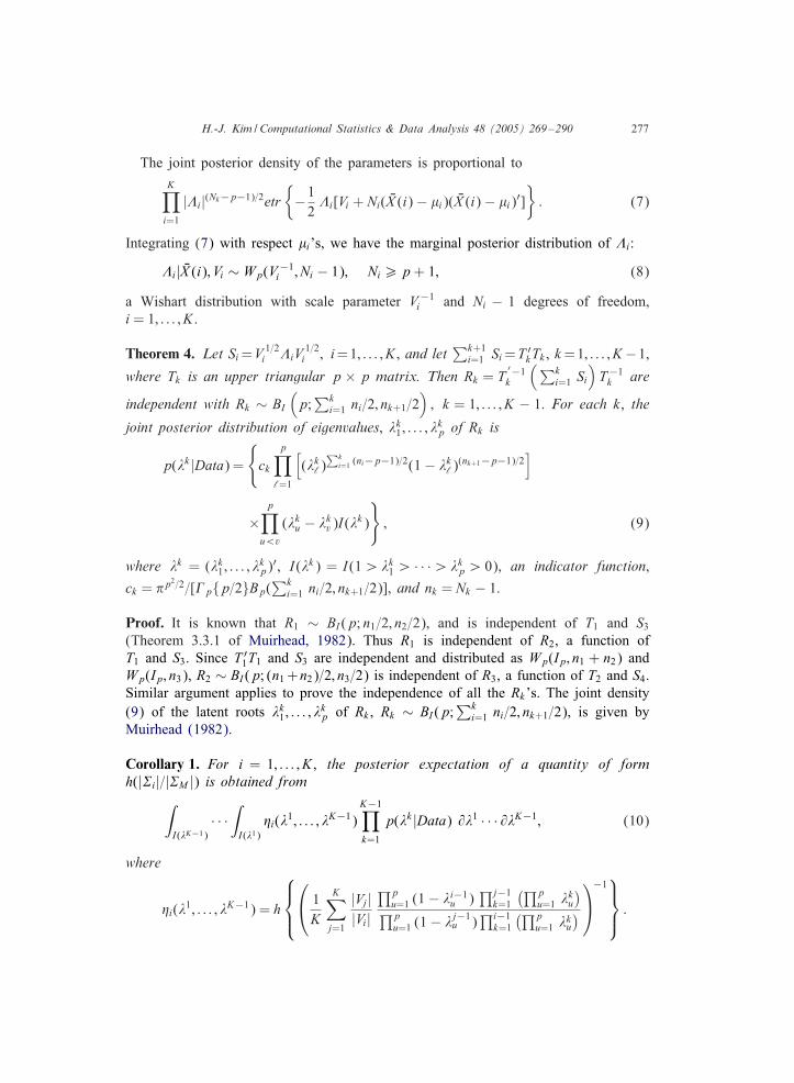
The joint posterior density of the parameters is proportional toK∏i=1

|%i|(Nk−p−1)=2etr{

−12%i[Vi + Ni( QX (i) − $i)( QX (i) − $i)′]

}: (7)

Integrating (7) with respect $i’s, we have the marginal posterior distribution of %i:

%i| QX (i); Vi ∼ Wp(V−1i ; Ni − 1); Ni¿p + 1; (8)

a Wishart distribution with scale parameter V−1i and Ni − 1 degrees of freedom,

i = 1; : : : ; K .

Theorem 4. Let Si =V 1=2i %iV

1=2i ; i=1; : : : ; K , and let

∑k+1i=1 Si =T ′

kTk , k =1; : : : ; K −1,

where Tk is an upper triangular p × p matrix. Then Rk = T′−1k

(∑ki=1 Si

)T−1k are

independent with Rk ∼ BI

(p;∑k

i=1 ni=2; nk+1=2); k = 1; : : : ; K − 1. For each k, the

joint posterior distribution of eigenvalues, -k1 ; : : : ; -

kp of Rk is

p(-k |Data) =

{ck

p∏‘=1

[(-k

‘)∑k

i=1 (ni−p−1)=2(1 − -k‘)

(nk+1−p−1)=2]

×p∏

u¡v

(-ku − -k

v)I(-k)

}; (9)

where -k = (-k1 ; : : : ; -

kp)′, I(-k) = I(1¿-k

1 ¿ · · ·¿-kp ¿ 0), an indicator function,

ck = 0p2=2=[1p{p=2}Bp(∑k

i=1 ni=2; nk+1=2)], and nk = Nk − 1.

Proof. It is known that R1 ∼ BI (p; n1=2; n2=2), and is independent of T1 and S3

(Theorem 3.3.1 of Muirhead, 1982). Thus R1 is independent of R2, a function ofT1 and S3. Since T ′

1T1 and S3 are independent and distributed as Wp(Ip; n1 + n2) andWp(Ip; n3), R2 ∼ BI (p; (n1 +n2)=2; n3=2) is independent of R3, a function of T2 and S4.Similar argument applies to prove the independence of all the Rk ’s. The joint density(9) of the latent roots -k

1 ; : : : ; -kp of Rk , Rk ∼ BI (p;

∑ki=1 ni=2; nk+1=2), is given by

Muirhead (1982).

Corollary 1. For i = 1; : : : ; K , the posterior expectation of a quantity of formh(|"i|=|"M |) is obtained from∫

I(-K−1)· · ·

∫I(-1)

3i(-1; : : : ; -K−1)K−1∏k=1

p(-k |Data) @-1 · · · @-K−1; (10)

where

3i(-1; : : : ; -K−1) = h

1

K

K∑j=1

|Vj||Vi|

∏pu=1 (1 − -i−1

u )∏j−1

k=1

(∏pu=1 -k

u

)∏p

u=1 (1 − -j−1u )

∏i−1k=1

(∏pu=1 -k

u

)

−1 :


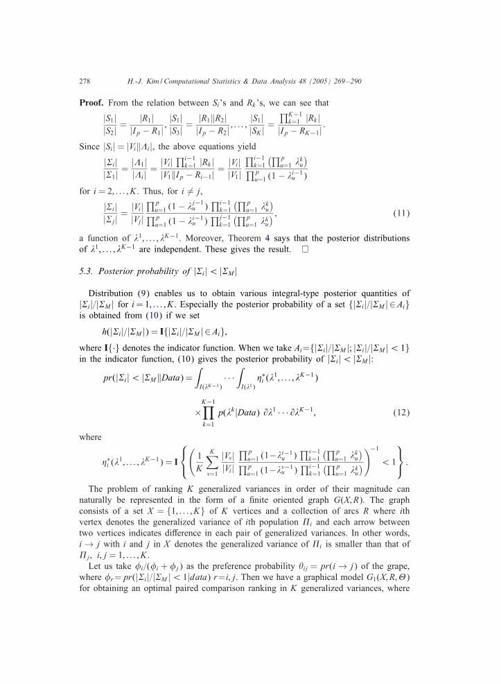
Proof. From the relation between Si’s and Rk ’s, we can see that

|S1||S2| =

|R1||Ip − R1| ;

|S1||S3| =

|R1‖R2||Ip − R2| ; : : : ;

|S1||SK | =

∏K−1k=1 |Rk |

|Ip − RK−1| :

Since |Si| = |Vi‖%i|, the above equations yield

|"i||"1| =

|%1||%i| =

|Vi|∏i−1

k=1 |Rk ||V1‖Ip − Ri−1| =

|Vi||V1|

∏i−1k=1

(∏pu=1 -k

u

)∏p

u=1 (1 − -i−1u )

for i = 2; : : : ; K . Thus, for i �= j,

|"i||"j| =

|Vi||Vj|

∏pu=1 (1 − -j−1

u )∏i−1

k=1

(∏pu=1 -k

u

)∏p

u=1 (1 − -i−1u )

∏j−1k=1

(∏pu=1 -k

u

) ; (11)

a function of -1; : : : ; -K−1. Moreover, Theorem 4 says that the posterior distributionsof -1; : : : ; -K−1 are independent. These gives the result.

5.3. Posterior probability of |"i|¡ |"M |

Distribution (9) enables us to obtain various integral-type posterior quantities of|"i|=|"M | for i = 1; : : : ; K . Especially the posterior probability of a set {|"i|=|"M | ∈Ai}is obtained from (10) if we set

h(|"i|=|"M |) = I{|"i|=|"M | ∈Ai};where I{·} denotes the indicator function. When we take Ai={|"i|=|"M |; |"i|=|"M |¡ 1}in the indicator function, (10) gives the posterior probability of |"i|¡ |"M |:

pr(|"i|¡ |"M‖Data) =∫I(-K−1)

· · ·∫I(-1)

3∗i (-

1; : : : ; -K−1)

×K−1∏k=1

p(-k |Data) @-1 · · · @-K−1; (12)

where

3∗i (-

1; : : : ; -K−1) = I

(

1K

K∑5=1

|V5||Vi|

∏pu=1 (1−-i−1

u )∏5−1

k=1

(∏pu=1 -k

u

)∏p

u=1 (1−-5−1u )

∏i−1k=1

(∏pu=1 -k

u

))−1

¡ 1

:

The problem of ranking K generalized variances in order of their magnitude cannaturally be represented in the form of a 1nite oriented graph G(X; R). The graphconsists of a set X = {1; : : : ; K} of K vertices and a collection of arcs R where ithvertex denotes the generalized variance of ith population �i and each arrow betweentwo vertices indicates diJerence in each pair of generalized variances. In other words,i → j with i and j in X denotes the generalized variance of �i is smaller than that of�j; i; j = 1; : : : ; K .

Let us take �i=(�i + �j) as the preference probability �ij = pr(i → j) of the grape,where �r=pr(|"i|=|"M |¡ 1|data) r=i; j. Then we have a graphical model G1(X; R;�)for obtaining an optimal paired comparison ranking in K generalized variances, where


�={�ij}; i; j=1; : : : ; K . The advantage of the parameterization is that �=(�1; : : : ; �K)is in terms of the set of K generalized variances, whereas the parameterization � ofthe model is in terms of the K(K−1)=2 paired comparisons. Moreover, it is straightfor-ward to see from Theorem 3 that the graphical model G1(X; R;�) satis1es the strongstochastic transitivity condition C2 in (2): for �ij¿ 1

2 implies �i¿�j which in turnimplies �i‘¿ �j‘ in that �ij is monotone increasing in �i. The true ranking of thegeneralized variances determined by � is precisely the ranking determined by �.

An analytic evaluation of the probability �ij is not available because the posteriordistribution

∏K−1k=1 p(-k |Data) in (12) is complicated. In this regard, a Monte-Carlo

method, in particular, a variant of weighted Monte-Carlo approach by Chen and Shao(1999) may naturally serve as an alternative solution for calculating the probability.The approach will be described in the next section.

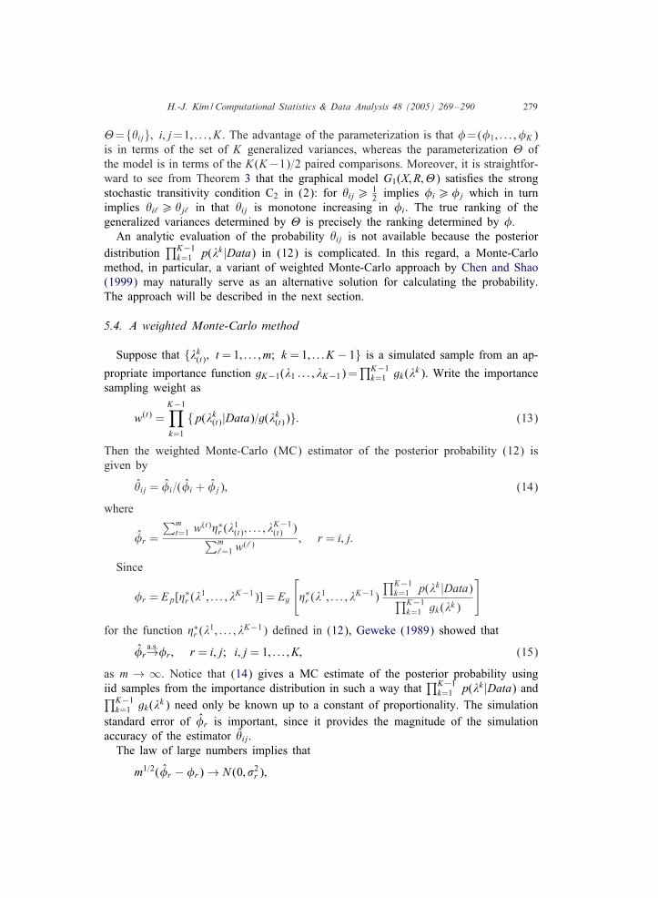
5.4. A weighted Monte-Carlo method

Suppose that {-k(t); t = 1; : : : ; m; k = 1; : : : K − 1} is a simulated sample from an ap-

propriate importance function gK−1(-1 : : : ; -K−1) =∏K−1

k=1 gk(-k). Write the importancesampling weight as

w(t) =K−1∏k=1

{p(-k(t)|Data)=g(-k

(t))}: (13)

Then the weighted Monte-Carlo (MC) estimator of the posterior probability (12) isgiven by

�ij = �i=(�i + �j); (14)

where

�r =

∑mt=1 w(t)3∗

r (-1(t); : : : ; -

K−1(t) )∑m

‘=1 w(‘)

; r = i; j:

Since

�r = Ep[3∗r (-

1; : : : ; -K−1)] = Eg

[3∗r (-

1; : : : ; -K−1)∏K−1

k=1 p(-k |Data)∏K−1k=1 gk(-k)

]

for the function 3∗r (-

1; : : : ; -K−1) de1ned in (12), Geweke (1989) showed that

�ra:s:→�r; r = i; j; i; j = 1; : : : ; K; (15)

as m → ∞. Notice that (14) gives a MC estimate of the posterior probability usingiid samples from the importance distribution in such a way that

∏K−1k=1 p(-k |Data) and∏K−1

k=1 gk(-k) need only be known up to a constant of proportionality. The simulationstandard error of �r is important, since it provides the magnitude of the simulationaccuracy of the estimator �ij.

The law of large numbers implies that

m1=2(�r − �r) → N (0; 92r );


where 92r =92

Vr=S2

r and it can be estimated by 92r = 92

Vr =Sr2 with Sr =1=m

∑mt=1 w

(t) and92Vr = 1=m

∑mt=1(w

(t)3∗r (-

1(t); : : : ; -

K−1(t) ) − w(t)�r)2.

Thus, from Rao (1973, p. 441), approximate distribution of �ij is

9−1(ij) m1=2(�ij − �ij) → N (0; 1);

where

92(ij) =∑r=i; j

∑r′=i; j

@�ij

@�r

@�ij

@�r′9rr′

provided 92m(ij) �= 0 when the true values of the parameters are substituted for �r ,

r= i; j. 9rr′ is covariance of m1=2(�r −�r) and m1=2(�r′ −�r′), and it can be estimatedby ˆCovrr′ =Sr

2, where

ˆCovrr′ = 1=mm∑

t=1

(w(t)3∗r (-

1(t); : : : ; -

K−1(t) ) − w(t)�r)(w(t)3∗

r′(-1(t); : : : ; -

K−1(t) )

−w(t)�r′):

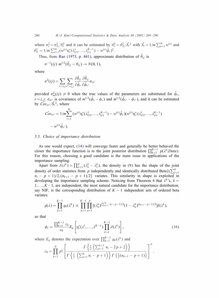
5.5. Choice of importance distribution

As one would expect, (14) will converge faster and generally be better behaved thecloser the importance function is to the joint posterior distribution

∏K−1k=1 p(-k |Data).

For this reason, choosing a good candidate is the main issue in applications of theimportance sampling.

Apart from J (-k) =∏p

u¡v (-ku − -k

v), the density in (9) has the shape of the jointdensity of order statistics from p independently and identically distributed Beta{(

∑ki=1

ni − p + 1)=2; (nk+1 − p + 1)=2} variates. This similarity in shape is exploited indeveloping the importance sampling scheme. Noticing from Theorem 4 that -k ’s, k =1; : : : ; K−1, are independent, the most natural candidate for the importance distribution,say NIF, is the corresponding distribution of K − 1 independent sets of ordered betavariates:

g(-) =K−1∏k=1

gk(-k) ˙K−1∏k=1

p∏u=1

[(-ku)

(∑k

i=1 ni−p−1)=2(1 − -ku)

(nk+1−p−1)=2]I(-k);

so that

�r =∏K−1

k=1 ckc0

Eg

[3∗r (-

1; : : : ; -K−1)K−1∏k=1

J (-k)

]; (16)

where Eg denotes the expectation over∏K−1

k=1 gk(-k) and

c0 =�∏

k=1

p!

1

{12

(∑k+1i=1 ni − 2p + 2

)}1{

12

(∑ki=1 ni − p + 1

)}1{

12 (nk+1 − p + 1)

}

p

:


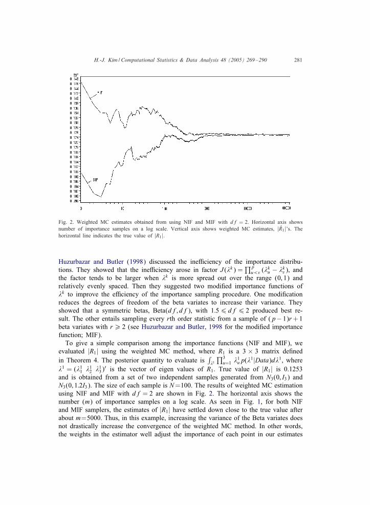
Fig. 2. Weighted MC estimates obtained from using NIF and MIF with df = 2. Horizontal axis showsnumber of importance samples on a log scale. Vertical axis shows weighted MC estimates, |R1|’s. Thehorizontal line indicates the true value of |R1|.

Huzurbazar and Butler (1998) discussed the ineKciency of the importance distribu-tions. They showed that the ineKciency arose in factor J (-k) =

∏pu¡v (-k

u − -kv), and

the factor tends to be larger when -k is more spread out over the range (0; 1) andrelatively evenly spaced. Then they suggested two modi1ed importance functions of-k to improve the eKciency of the importance sampling procedure. One modi1cationreduces the degrees of freedom of the beta variates to increase their variance. Theyshowed that a symmetric betas, Beta(df; df), with 1:56df6 2 produced best re-sult. The other entails sampling every rth order statistic from a sample of (p−1)r +1beta variates with r¿ 2 (see Huzurbazar and Butler, 1998 for the modi1ed importancefunction; MIF).

To give a simple comparison among the importance functions (NIF and MIF), weevaluated |R1| using the weighted MC method, where R1 is a 3 × 3 matrix de1nedin Theorem 4. The posterior quantity to evaluate is

∫-1

∏3u=1 -1

up(-1|Data)d-1, where-1 = (-1

1 -12 -1

3)′ is the vector of eigen values of R1. True value of |R1| is 0.1253

and is obtained from a set of two independent samples generated from N3(0; I3) andN3(0; 1:2I3). The size of each sample is N=100. The results of weighted MC estimationusing NIF and MIF with df = 2 are shown in Fig. 2. The horizontal axis shows thenumber (m) of importance samples on a log scale. As seen in Fig. 1, for both NIFand MIF samplers, the estimates of |R1| have settled down close to the true value afterabout m=5000. Thus, in this example, increasing the variance of the Beta variates doesnot drastically increase the convergence of the weighted MC method. In other words,the weights in the estimator well adjust the importance of each point in our estimates


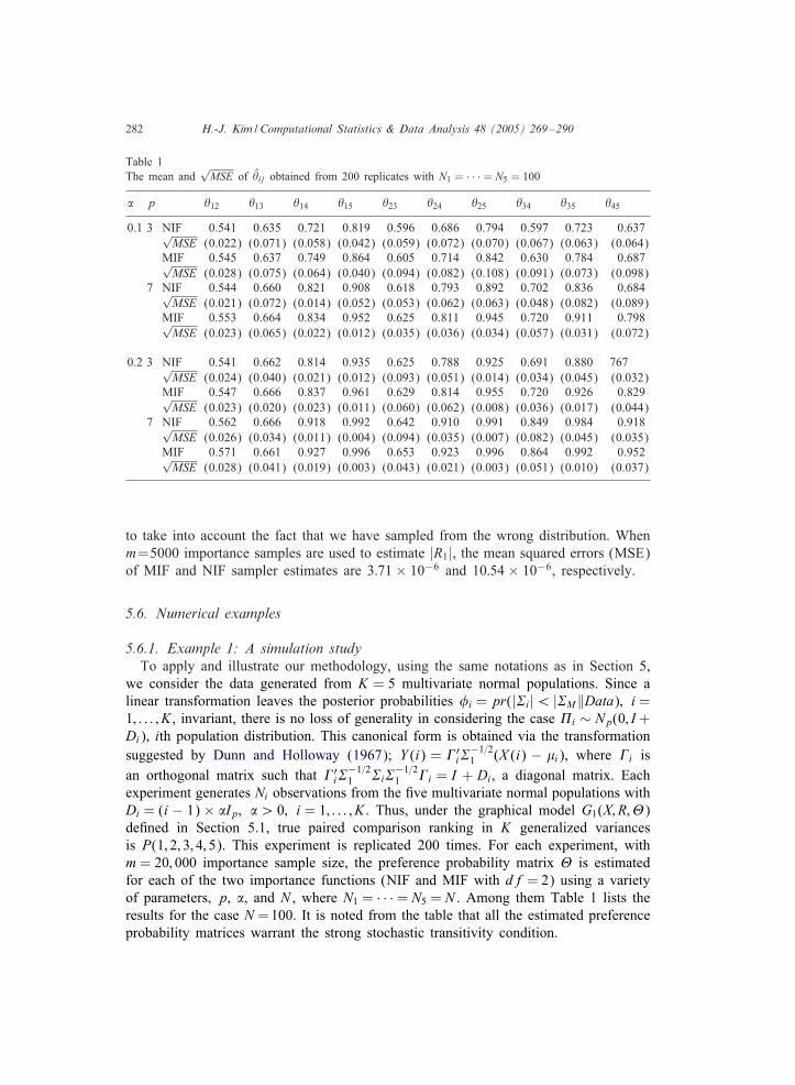
Table 1The mean and

√MSE of �ij obtained from 200 replicates with N1 = · · · = N5 = 100

= p �12 �13 �14 �15 �23 �24 �25 �34 �35 �45

0.1 3 NIF 0.541 0.635 0.721 0.819 0.596 0.686 0.794 0.597 0.723 0.637√MSE (0.022) (0.071) (0.058) (0.042) (0.059) (0.072) (0.070) (0.067) (0.063) (0.064)

MIF 0.545 0.637 0.749 0.864 0.605 0.714 0.842 0.630 0.784 0.687√MSE (0.028) (0.075) (0.064) (0.040) (0.094) (0.082) (0.108) (0.091) (0.073) (0.098)

7 NIF 0.544 0.660 0.821 0.908 0.618 0.793 0.892 0.702 0.836 0.684√MSE (0.021) (0.072) (0.014) (0.052) (0.053) (0.062) (0.063) (0.048) (0.082) (0.089)

MIF 0.553 0.664 0.834 0.952 0.625 0.811 0.945 0.720 0.911 0.798√MSE (0.023) (0.065) (0.022) (0.012) (0.035) (0.036) (0.034) (0.057) (0.031) (0.072)

0.2 3 NIF 0.541 0.662 0.814 0.935 0.625 0.788 0.925 0.691 0.880 767√MSE (0.024) (0.040) (0.021) (0.012) (0.093) (0.051) (0.014) (0.034) (0.045) (0.032)

MIF 0.547 0.666 0.837 0.961 0.629 0.814 0.955 0.720 0.926 0.829√MSE (0.023) (0.020) (0.023) (0.011) (0.060) (0.062) (0.008) (0.036) (0.017) (0.044)

7 NIF 0.562 0.666 0.918 0.992 0.642 0.910 0.991 0.849 0.984 0.918√MSE (0.026) (0.034) (0.011) (0.004) (0.094) (0.035) (0.007) (0.082) (0.045) (0.035)

MIF 0.571 0.661 0.927 0.996 0.653 0.923 0.996 0.864 0.992 0.952√MSE (0.028) (0.041) (0.019) (0.003) (0.043) (0.021) (0.003) (0.051) (0.010) (0.037)

to take into account the fact that we have sampled from the wrong distribution. Whenm=5000 importance samples are used to estimate |R1|, the mean squared errors (MSE)of MIF and NIF sampler estimates are 3:71 × 10−6 and 10:54 × 10−6, respectively.

5.6. Numerical examples

5.6.1. Example 1: A simulation studyTo apply and illustrate our methodology, using the same notations as in Section 5,

we consider the data generated from K = 5 multivariate normal populations. Since alinear transformation leaves the posterior probabilities �i = pr(|"i|¡ |"M‖Data); i =1; : : : ; K , invariant, there is no loss of generality in considering the case �i ∼ Np(0; I +Di), ith population distribution. This canonical form is obtained via the transformationsuggested by Dunn and Holloway (1967); Y (i) = 1′

i"−1=21 (X (i) − $i), where 1i is

an orthogonal matrix such that 1′i"

−1=21 "i"

−1=21 1i = I + Di, a diagonal matrix. Each

experiment generates Ni observations from the 1ve multivariate normal populations withDi = (i − 1) × =Ip; =¿ 0; i = 1; : : : ; K . Thus, under the graphical model G1(X; R;�)de1ned in Section 5.1, true paired comparison ranking in K generalized variancesis P(1; 2; 3; 4; 5). This experiment is replicated 200 times. For each experiment, withm = 20; 000 importance sample size, the preference probability matrix � is estimatedfor each of the two importance functions (NIF and MIF with df = 2) using a varietyof parameters, p, =, and N , where N1 = · · · = N5 = N . Among them Table 1 lists theresults for the case N =100. It is noted from the table that all the estimated preferenceprobability matrices warrant the strong stochastic transitivity condition.


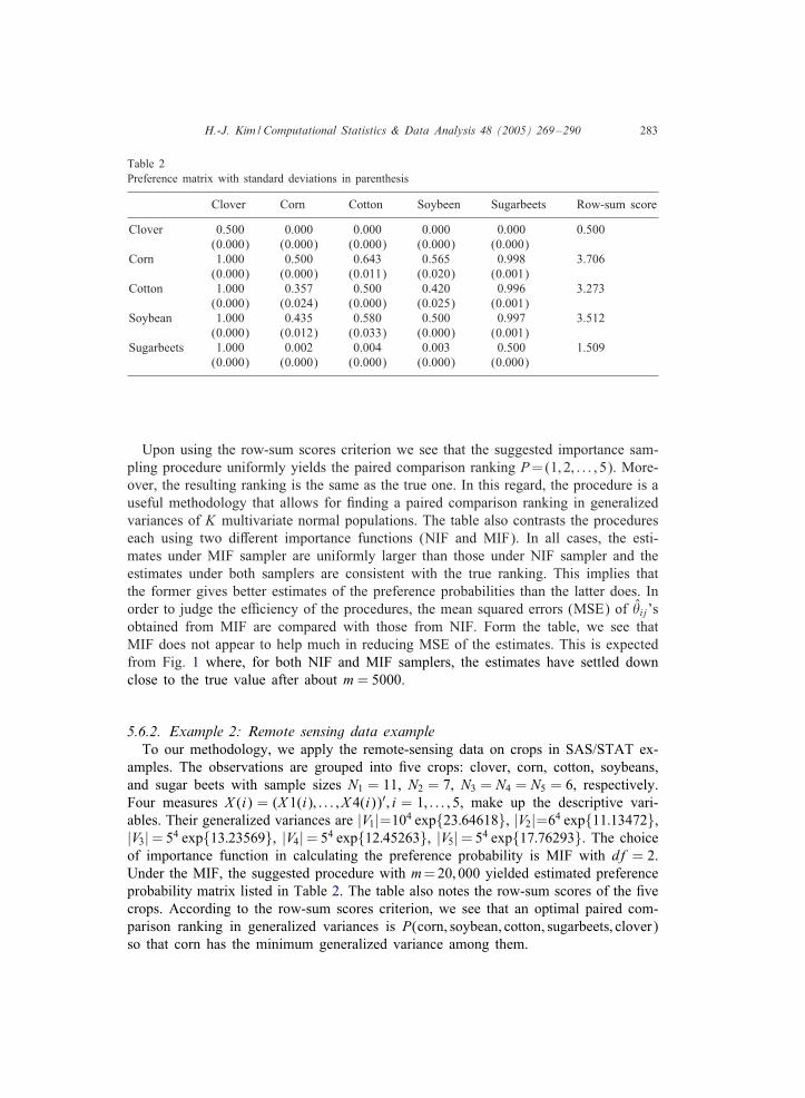
Table 2Preference matrix with standard deviations in parenthesis

Clover Corn Cotton Soybeen Sugarbeets Row-sum score

Clover 0.500 0.000 0.000 0.000 0.000 0.500(0.000) (0.000) (0.000) (0.000) (0.000)

Corn 1.000 0.500 0.643 0.565 0.998 3.706(0.000) (0.000) (0.011) (0.020) (0.001)

Cotton 1.000 0.357 0.500 0.420 0.996 3.273(0.000) (0.024) (0.000) (0.025) (0.001)

Soybean 1.000 0.435 0.580 0.500 0.997 3.512(0.000) (0.012) (0.033) (0.000) (0.001)

Sugarbeets 1.000 0.002 0.004 0.003 0.500 1.509(0.000) (0.000) (0.000) (0.000) (0.000)

Upon using the row-sum scores criterion we see that the suggested importance sam-pling procedure uniformly yields the paired comparison ranking P=(1; 2; : : : ; 5). More-over, the resulting ranking is the same as the true one. In this regard, the procedure is auseful methodology that allows for 1nding a paired comparison ranking in generalizedvariances of K multivariate normal populations. The table also contrasts the procedureseach using two diJerent importance functions (NIF and MIF). In all cases, the esti-mates under MIF sampler are uniformly larger than those under NIF sampler and theestimates under both samplers are consistent with the true ranking. This implies thatthe former gives better estimates of the preference probabilities than the latter does. Inorder to judge the eKciency of the procedures, the mean squared errors (MSE) of �ij’sobtained from MIF are compared with those from NIF. Form the table, we see thatMIF does not appear to help much in reducing MSE of the estimates. This is expectedfrom Fig. 1 where, for both NIF and MIF samplers, the estimates have settled downclose to the true value after about m = 5000.

5.6.2. Example 2: Remote sensing data exampleTo our methodology, we apply the remote-sensing data on crops in SAS/STAT ex-

amples. The observations are grouped into 1ve crops: clover, corn, cotton, soybeans,and sugar beets with sample sizes N1 = 11, N2 = 7, N3 = N4 = N5 = 6, respectively.Four measures X (i) = (X 1(i); : : : ; X 4(i))′; i = 1; : : : ; 5, make up the descriptive vari-ables. Their generalized variances are |V1|=104 exp{23:64618}, |V2|=64 exp{11:13472},|V3| = 54 exp{13:23569}, |V4| = 54 exp{12:45263}, |V5| = 54 exp{17:76293}. The choiceof importance function in calculating the preference probability is MIF with df = 2.Under the MIF, the suggested procedure with m=20; 000 yielded estimated preferenceprobability matrix listed in Table 2. The table also notes the row-sum scores of the 1vecrops. According to the row-sum scores criterion, we see that an optimal paired com-parison ranking in generalized variances is P(corn; soybean; cotton; sugarbeets; clover)so that corn has the minimum generalized variance among them.


6. Application of ranking in products of normal means

6.1. Graphical model

As indicated in Section 1, the estimate of a product of normal means has been ap-plied in many environmental statistical problems. In this section, we consider Bayesianinference concerning the paired comparisons ranking in products of s normal means, k , k=1; : : : ; K among K populations by using G2(X; R;�). Let X ={1; 2; : : : ; K} be theset of vertices whose element correspond to index of the product of s normal meansof each population. Element �ij of � denotes the posterior preference probability,

pr(i → j) =pr( i − M ¡ 0|data)

pr( i − M ¡ 0|data) + pr( j − M ¡ 0|data) ; i �= j;

so that the graphical model warrants the strong stochastic transitivity condition C2 byTheorem 3. Here M is the mean of k ’s.

When s = 2, estimating k can be recognized as the determination of an area of arectangular based measurements of length and width in kth population. For s = 3, k

can be viewed as the volume of a cuboid when the length, width, and height representthe means of three normal random variables. An example is in the assessment of riskdue to exposure to radiation or various pollutants. Assume that the does per unit time,the units of time per day, and number of days during which an individual is exposedare three independent normal random variables. The total exposure is the product ofthree means.

6.2. Posterior preference probability

Suppose that X‘1(k); : : : ; X‘N‘k(k) are independent sample of ‘th variable from kth

normal population having distribution N ($‘(k); 92‘(k)) with $‘(k)¿ 0, for ‘= 1; : : : ; s;

k=1; : : : ; K . The parameters of interest are 1 =∏s

‘=1 $‘(1), 2 =∏s

‘=1 $‘(2); : : : ; K =∏s‘=1 $‘(K), the products of s independent normal means of K experimental sites

(or populations).Assuming priori independence of $‘(k)’s and 92

‘(k)’s, we take a reference prior for$‘(k)’s and log 92

‘(k)’s, that is

0($‘(k); 92‘(k); ‘ = 1; : : : ; s; k = 1; : : : ; K)

˙K∏

k=1

s∏‘=1

9−2‘ (k)

1 + $2

‘(k)∑‘′ �=‘

$−2‘′ (k)

1=2

:

Here, for the prior of the product of $‘(k)’s, we use a reference prior developed bySun and Ye (1995). Our interest in this example is the optimal ranking in the relativemagnitudes of the products of the s means among K diJerent experimental sites. Inparticular, we want to obtain the preference probabilities matrix � = {�ij}.


It is straightforward to see that the joint posterior distribution of $‘(k)’s is

p($‘(k); k = 1; : : : ; K ; ‘ = 1; : : : ; s|Data)

˙s∏

‘=1

K∏k=1

1 + $2

‘(k)∑‘′ �=‘

$−2‘′ (k)

1=2

×1 +

{$‘(k) − QX ‘(k)s‘(k)=

√N‘k

}2

=(N‘k − 1)

−N‘k =2

(17)

for $‘(k)¿ 0, where QX ‘(k) =∑N‘k

u=1 X‘u(k)=n‘k , and s2‘(k) =∑N‘k

u=1 (X‘u(k) − QX ‘(k))2=(N‘k − 1). Thus

�ij =�∗

i

�∗i + �∗

j; i; j = 1; : : : ; K;

where �∗r = Ep[I{ i − M ¡ 0}|Data], r = i; j, and the expectation Ep is taken with

respect to the joint posterior distribution (17), and I(·) is the indicator function.Assume that {$(t)

‘ (k); t=1; : : : ; m; k= i; : : : ; K ; ‘=1; : : : ; s} is a random sample froman importance function g($‘(k); k = 1; : : : ; K ; ‘ = 1; : : : ; s) of (17). Then, from theweighted MC method described in Section 5.4, an estimate of �ij can be obtained by

�ij =�∗

i

�∗i + �∗

j

; (18)

where

�∗r =

∑mt=1 w(t)I

{∏s‘ $(t)

‘ (r) −∑Kk=1

(∏s‘ $(t)

‘ (k))=K ¡ 0

}∑m

‘=1 w(‘); r = i; j

and

w(t) =p($(t)

‘ (k); k = i; : : : ; K ; ‘ = 1; : : : ; s|Data)

g($(t)‘ (k); k = 1; : : : ; K ; ‘ = 1; : : : ; s)

; t = 1; : : : ; m

are the important sampling weights. Asymptotic properties of �∗r and �ij can be easily

derived by using analogous derivation in Section 5.2.

6.3. Numerical examples

6.3.1. Example 3: Multiple comparisons in normal meansIn this example, we consider the optimal paired comparison ranking in K independent

normal means under the graphical model G2(X; R;�), and compare with the results ofthe Duncan multiple range test and the Tukey’s test. Suppose that Nk independent


Table 3The mean and standard deviation of �ij obtained from 100 replicates

Nk �12 �13 �14 �15 �16 �23 �24 �25

20 Mean 0.604 0.641 0.669 0.891 0.999 0.540 0.571 0.987s.d. (0.031) (0.021) (0.019) (0.012) (0.021) (0.024) (0.027) (0.015)

50 Mean 0.613 0.709 0.882 0.901 0.999 0.572 0.876 0.989s.d. (0.036) (0.042) (0.024) (0.012) (0.009) (0.025) (0.026) (0.008)

100 Mean 0.637 0.767 0.911 0.999 1.000 0.655 0.898 0.999s.d. (0.028) (0.013) (0.011) (0.007) (0.001) (0.026) (0.013) (0.001)

�26 �34 �35 �36 �45 �46 �56

0.998 0.531 0.954 0.998 0.924 0.993 0.889(0.003) (0.026) (0.013) (0.001) (0.005) (0.001) (0.015)0.999 0.788 0.978 0.998 0.982 0.998 0.917

(0.001) (0.017) (0.003) (0.005) (0.002) (0.001) (0.08)1.000 0.868 0.998 1.000 0.987 0.999 0.996

(0.001) (0.011) (0.003) (0.000) (0.012) (0.001) (0.005)

observations X5k (k), 5k = 1; : : : ; Nk , are drawn from the normal population N ($k ; 92k)

for k = 1; : : : ; K . We take a uniform prior for $1; : : : ; $K , log 921 ; : : : ; log 92

K , that is0($1; : : : ; $K ; 92

1 ; : : : ; 92K) ˙

∏Kk=1 9−2

k . The joint posterior distribution of $1; : : : ; $K isgiven by

p($k ; k = 1; : : : ; K |Data) ˙K∏

k=1

(1 +

{$k − QX k

sk=√Nk

}2

=(Nk − 1)

)−Nk =2

(19)

a product of independent t-density functions with the mean QX k , the scale parametersk=

√Nk , and Nk − 1 degrees of freedom for k = 1; : : : ; K .

For illustrative purpose, we drew Nk independent observations from N ($k ; 92k), where

Nk = 20; 50; 100, $k = 1 + 0:5(k − 1), and 92k = 2 + 0:1(k − 1) for k = 1; : : : ; 6, so that

K = 6 and true ranking in the ascending order in magnitudes of K normal means isP = (1; 2; 3; 4; 5; 6).

Using 100 replications of simulated samples {$(t)k ; t = 1; : : : ; 10; 000; k = 1; : : : ; 6}

from (19), we obtained the means and standard deviations of MC estimates of �ij,i �= j; i; j = 1; : : : ; 6. They are tabulated in Table 3.

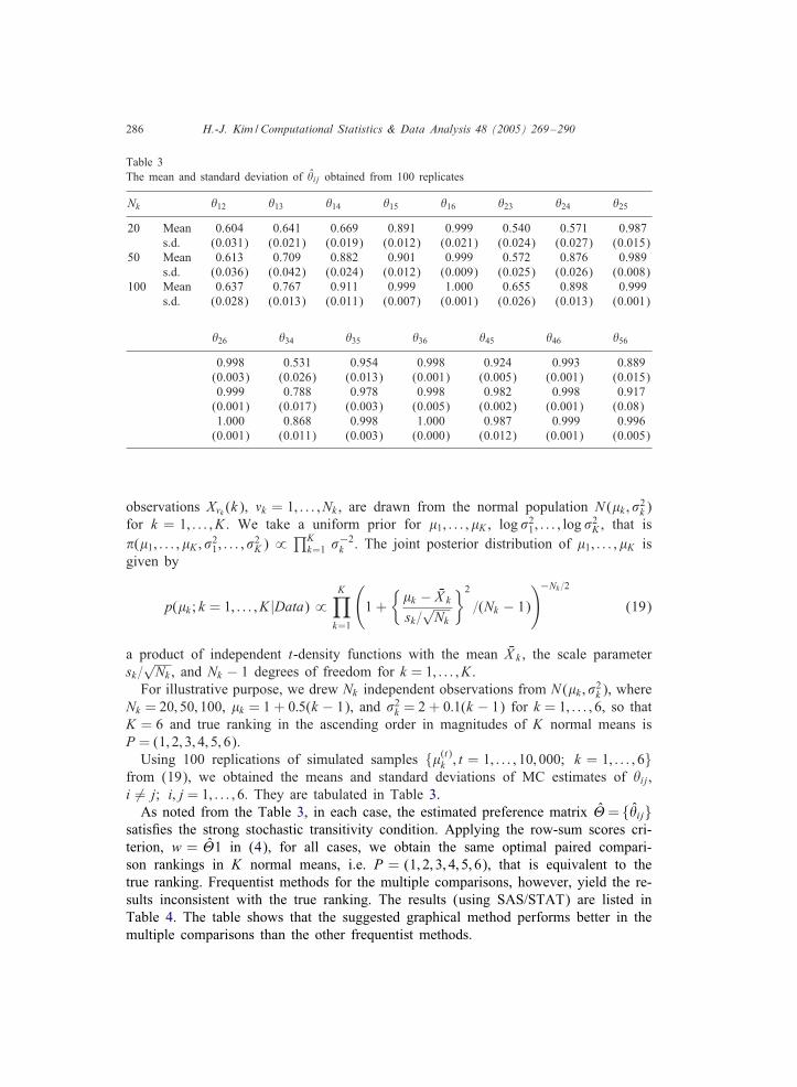
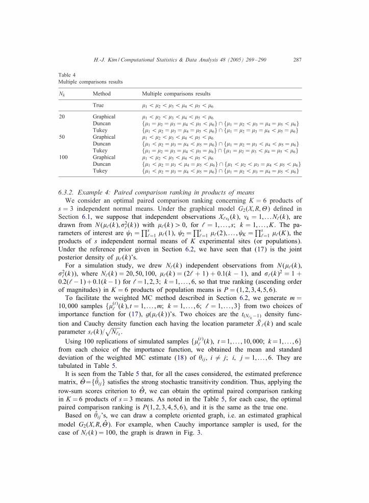
As noted from the Table 3, in each case, the estimated preference matrix �= {�ij}satis1es the strong stochastic transitivity condition. Applying the row-sum scores cri-terion, w = �1 in (4), for all cases, we obtain the same optimal paired compari-son rankings in K normal means, i.e. P = (1; 2; 3; 4; 5; 6), that is equivalent to thetrue ranking. Frequentist methods for the multiple comparisons, however, yield the re-sults inconsistent with the true ranking. The results (using SAS/STAT) are listed inTable 4. The table shows that the suggested graphical method performs better in themultiple comparisons than the other frequentist methods.


Table 4Multiple comparisons results

Nk Method Multiple comparisons results

True $1 ¡$2 ¡$3 ¡$4 ¡$5 ¡$6

20 Graphical $1 ¡$2 ¡$3 ¡$4 ¡$5 ¡$6Duncan {$1 = $2 = $3 = $4 ¡$5 ¡$6} ∩ {$1 = $2 ¡$3 = $4 = $5 ¡$6}Tukey {$1 ¡$2 = $3 = $4 = $5 ¡$6} ∩ {$1 = $2 = $3 = $4 ¡$5 = $6}

50 Graphical $1 ¡$2 ¡$3 ¡$4 ¡$5 ¡$6Duncan {$1 ¡$2 = $3 = $4 ¡$5 = $6} ∩ {$1 = $2 = $3 ¡$4 ¡$5 = $6}Tukey {$1 = $2 = $3 = $4 ¡$5 = $6} ∩ {$1 = $2 = $3 ¡$4 = $5 ¡$6}

100 Graphical $1 ¡$2 ¡$3 ¡$4 ¡$5 ¡$6Duncan {$1 ¡$2 = $3 ¡$4 = $5 ¡$6} ∩ {$1 ¡$2 ¡$3 = $4 ¡$5 ¡$6}Tukey {$1 ¡$2 = $3 = $4 ¡$5 = $6} ∩ {$1 = $2 ¡$3 = $4 = $5 ¡$6}

6.3.2. Example 4: Paired comparison ranking in products of meansWe consider an optimal paired comparison ranking concerning K = 6 products of

s = 3 independent normal means. Under the graphical model G2(X; R;�) de1ned inSection 6.1, we suppose that independent observations X‘5k (k), 5k = 1; : : : N‘(k), aredrawn from N ($‘(k); 92

‘(k)) with $‘(k)¿ 0, for ‘ = 1; : : : ; s; k = 1; : : : ; K . The pa-rameters of interest are 1 =

∏s‘=1 $‘(1), 2 =

∏s‘=1 $‘(2); : : : ; K =

∏s‘=1 $‘(K), the

products of s independent normal means of K experimental sites (or populations).Under the reference prior given in Section 6.2, we have seen that (17) is the jointposterior density of $‘(k)’s.

For a simulation study, we drew N‘(k) independent observations from N ($‘(k);92‘(k)), where N‘(k) = 20; 50; 100, $‘(k) = (2‘ + 1) + 0:1(k − 1), and 9‘(k)2 = 1 +

0:2(‘−1)+0:1(k −1) for ‘=1; 2; 3; k =1; : : : ; 6; so that true ranking (ascending orderof magnitudes) in K = 6 products of population means is P = (1; 2; 3; 4; 5; 6).

To facilitate the weighted MC method described in Section 6.2, we generate m =10; 000 samples {$(t)

‘ (k); t = 1; : : : ; m; k = 1; : : : ; 6; ‘ = 1; : : : ; 3} from two choices ofimportance function for (17), g($‘(k))’s. Two choices are the t(N‘k −1) density func-tion and Cauchy density function each having the location parameter QX ‘(k) and scaleparameter s‘(k)=

√N‘k .

Using 100 replications of simulated samples {$(t)‘ (k); t=1; : : : ; 10; 000; k =1; : : : ; 6}

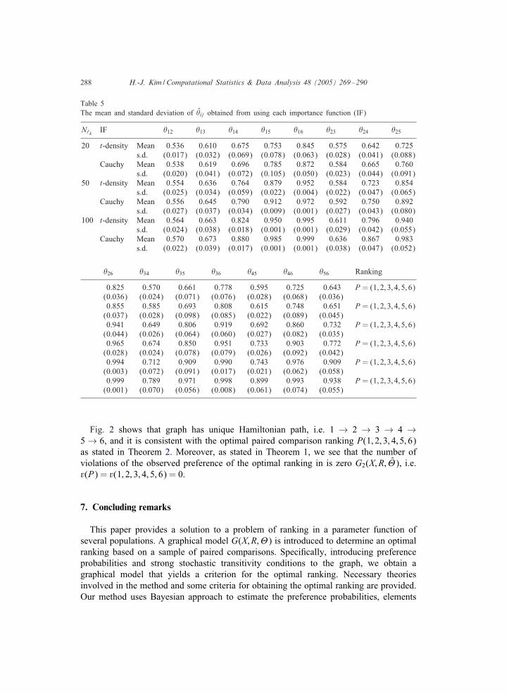
from each choice of the importance function, we obtained the mean and standarddeviation of the weighted MC estimate (18) of �ij, i �= j; i; j = 1; : : : ; 6. They aretabulated in Table 5.

It is seen from the Table 5 that, for all the cases considered, the estimated preferencematrix, �={�ij} satis1es the strong stochastic transitivity condition. Thus, applying therow-sum scores criterion to �, we can obtain the optimal paired comparison rankingin K = 6 products of s= 3 means. As noted in the Table 5, for each case, the optimalpaired comparison ranking is P(1; 2; 3; 4; 5; 6), and it is the same as the true one.

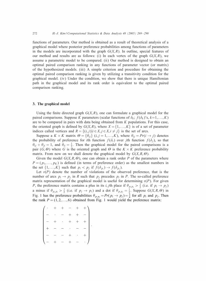
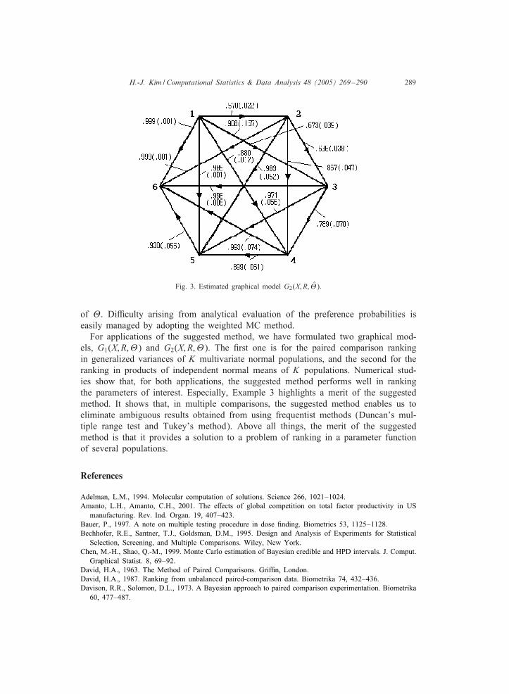
Based on �ij’s, we can draw a complete oriented graph, i.e. an estimated graphicalmodel G2(X; R; �). For example, when Cauchy importance sampler is used, for thecase of N‘(k) = 100, the graph is drawn in Fig. 3.


Table 5The mean and standard deviation of �ij obtained from using each importance function (IF)

N‘k IF �12 �13 �14 �15 �16 �23 �24 �25

20 t-density Mean 0.536 0.610 0.675 0.753 0.845 0.575 0.642 0.725s.d. (0.017) (0.032) (0.069) (0.078) (0.063) (0.028) (0.041) (0.088)

Cauchy Mean 0.538 0.619 0.696 0.785 0.872 0.584 0.665 0.760s.d. (0.020) (0.041) (0.072) (0.105) (0.050) (0.023) (0.044) (0.091)

50 t-density Mean 0.554 0.636 0.764 0.879 0.952 0.584 0.723 0.854s.d. (0.025) (0.034) (0.059) (0.022) (0.004) (0.022) (0.047) (0.065)

Cauchy Mean 0.556 0.645 0.790 0.912 0.972 0.592 0.750 0.892s.d. (0.027) (0.037) (0.034) (0.009) (0.001) (0.027) (0.043) (0.080)

100 t-density Mean 0.564 0.663 0.824 0.950 0.995 0.611 0.796 0.940s.d. (0.024) (0.038) (0.018) (0.001) (0.001) (0.029) (0.042) (0.055)

Cauchy Mean 0.570 0.673 0.880 0.985 0.999 0.636 0.867 0.983s.d. (0.022) (0.039) (0.017) (0.001) (0.001) (0.038) (0.047) (0.052)

�26 �34 �35 �36 �45 �46 �56 Ranking

0.825 0.570 0.661 0.778 0.595 0.725 0.643 P = (1; 2; 3; 4; 5; 6)(0.036) (0.024) (0.071) (0.076) (0.028) (0.068) (0.036)0.855 0.585 0.693 0.808 0.615 0.748 0.651 P = (1; 2; 3; 4; 5; 6)

(0.037) (0.028) (0.098) (0.085) (0.022) (0.089) (0.045)0.941 0.649 0.806 0.919 0.692 0.860 0.732 P = (1; 2; 3; 4; 5; 6)

(0.044) (0.026) (0.064) (0.060) (0.027) (0.082) (0.035)0.965 0.674 0.850 0.951 0.733 0.903 0.772 P = (1; 2; 3; 4; 5; 6)

(0.028) (0.024) (0.078) (0.079) (0.026) (0.092) (0.042)0.994 0.712 0.909 0.990 0.743 0.976 0.909 P = (1; 2; 3; 4; 5; 6)

(0.003) (0.072) (0.091) (0.017) (0.021) (0.062) (0.058)0.999 0.789 0.971 0.998 0.899 0.993 0.938 P = (1; 2; 3; 4; 5; 6)

(0.001) (0.070) (0.056) (0.008) (0.061) (0.074) (0.055)

Fig. 2 shows that graph has unique Hamiltonian path, i.e. 1 → 2 → 3 → 4 →5 → 6, and it is consistent with the optimal paired comparison ranking P(1; 2; 3; 4; 5; 6)as stated in Theorem 2. Moreover, as stated in Theorem 1, we see that the number ofviolations of the observed preference of the optimal ranking in is zero G2(X; R; �), i.e.v(P) = v(1; 2; 3; 4; 5; 6) = 0.

7. Concluding remarks

This paper provides a solution to a problem of ranking in a parameter function ofseveral populations. A graphical model G(X; R;�) is introduced to determine an optimalranking based on a sample of paired comparisons. Speci1cally, introducing preferenceprobabilities and strong stochastic transitivity conditions to the graph, we obtain agraphical model that yields a criterion for the optimal ranking. Necessary theoriesinvolved in the method and some criteria for obtaining the optimal ranking are provided.Our method uses Bayesian approach to estimate the preference probabilities, elements


Fig. 3. Estimated graphical model G2(X; R; �).

of �. DiKculty arising from analytical evaluation of the preference probabilities iseasily managed by adopting the weighted MC method.

For applications of the suggested method, we have formulated two graphical mod-els, G1(X; R;�) and G2(X; R;�). The 1rst one is for the paired comparison rankingin generalized variances of K multivariate normal populations, and the second for theranking in products of independent normal means of K populations. Numerical stud-ies show that, for both applications, the suggested method performs well in rankingthe parameters of interest. Especially, Example 3 highlights a merit of the suggestedmethod. It shows that, in multiple comparisons, the suggested method enables us toeliminate ambiguous results obtained from using frequentist methods (Duncan’s mul-tiple range test and Tukey’s method). Above all things, the merit of the suggestedmethod is that it provides a solution to a problem of ranking in a parameter functionof several populations.

References

Adelman, L.M., 1994. Molecular computation of solutions. Science 266, 1021–1024.Amanto, L.H., Amanto, C.H., 2001. The eJects of global competition on total factor productivity in US

manufacturing. Rev. Ind. Organ. 19, 407–423.Bauer, P., 1997. A note on multiple testing procedure in dose 1nding. Biometrics 53, 1125–1128.Bechhofer, R.E., Santner, T.J., Goldsman, D.M., 1995. Design and Analysis of Experiments for Statistical

Selection, Screening, and Multiple Comparisons. Wiley, New York.Chen, M.-H., Shao, Q.-M., 1999. Monte Carlo estimation of Bayesian credible and HPD intervals. J. Comput.

Graphical Statist. 8, 69–92.David, H.A., 1963. The Method of Paired Comparisons. GriKn, London.David, H.A., 1987. Ranking from unbalanced paired-comparison data. Biometrika 74, 432–436.Davison, R.R., Solomon, D.L., 1973. A Bayesian approach to paired comparison experimentation. Biometrika

60, 477–487.


Dunn, O.J., Holloway, L.N., 1967. The robustness of Hotelling’s T 2. J. Amer. Statist. Assoc. 62, 124–136.Fu, B., Beigel, R., Zhou, F., 2003. An O(2n) volume molecular algorithm for Hamiltonian path.

www.cis.temple.edu/∼beigel/papers.Geweke, J., 1989. Bayesian inference in econometrics models using Monte Carlo integration. Econometrica

57, 1340–1371.Gilbert, S., 2003. Distribution of rankings for groups exhibiting heteroscedasticity and correlation. J. Amer.

Statist. Assoc. 98, 147–157.Grizzle, J.E., Allen, D.M., 1969. Analysis of growth and does response curves. Biometrics 25, 357–382.Harary, F., Norman, R.Z., Cartwright, D., 1965. Structural Models: An Introduction to the Theory of Directed

Graphs. Wiley, New York.Hsu, J.C., 1996. Multiple Comparisons. Chapman & Hall, London.Huzurbazar, S., Butler, R.W., 1998. Importance sampling for p-value computations in multivariate tests. J.

Comput. Graphical Statist. 7, 342–355.Kendall, M.G., 1948. Rank Correlation Methods. Charles GriKn and Co., London.Kim, S., Nelson, B.L., 2001. A fully sequential selection procedure for indiJerence-zone selection in

simulation. Trans. Model. Comput. Simulation 11, 251–273.Luce, R.D., 1961 A choice theory analysis of similarity judgements. Psychometrika 26, 151–163.Muirhead, R.J., 1982. Aspects of Multivariate Statistical Theory. Wiley, New York.Pennello, G., 1997. The k-ratio multiple comparisons Bayes rule for the balanced two-way design. J. Amer.

Statist. Assoc. 92, 675–684.Press, S.J., 1982. Applied Multivariate Analysis. Krieger Publishing Co., Florida.Rao, C.R., 1973. Linear Statistical Inference and Its Applications. Wiley, New York.Rencher, A.C., 2002. Methods of Multivariate Analysis. Wiley, New York.Skiena, S., 1990. Implementing Discrete Mathematics: Combinatorics and Graph Theory with Mathematica.

Addison-Wesley, Reading, MA.Slater, P., 1961. Inconsistencies in a schedule of paired comparisons. Biometrika 48, 303–312.Sun, D., Ye, K., 1995. Reference prior Bayesian analysis for normal mean products. J. Amer. Statist. Assoc.

90, 589–597.

http://www.cis.temple.edu/~beigel/papers

a bayesian approach to paired comparison rankings based on a graphical model

Documents