9 recurrent quantum neural network and its applications€¦ · · 2015-08-139 recurrent quantum...
TRANSCRIPT
9 Recurrent Quantum Neural Network
and its Applications
Laxmidhar Behera, Indrani Kar, and Avshalom C. Elitzur
Summary. Although the biological body consists of many individual parts oragents, our experience is holistic. We suggest that collective response behavior isa key feature in intelligence. A nonlinear Schrodinger wave equation is used tomodel collective response behavior. It is shown that such a paradigm can naturallymake a model more intelligent. This aspect has been demonstrated through an ap-plication – intelligent filtering – where complex signals are denoised without anya priori knowledge about either signal or noise. Such a paradigm has also helpedus to model eye-tracking behavior. Experimental observations such as saccadic andsmooth-pursuit eye-movement behavior have been successfully predicted by thismodel.
9.1 Intelligence – Still Ill-Understood
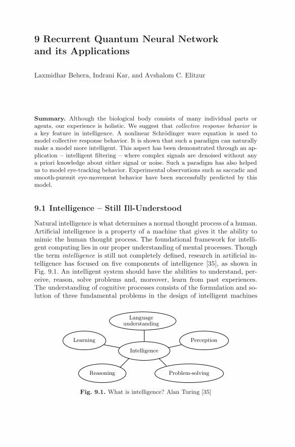
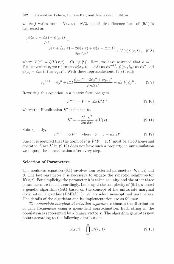
Natural intelligence is what determines a normal thought process of a human.Artificial intelligence is a property of a machine that gives it the ability tomimic the human thought process. The foundational framework for intelli-gent computing lies in our proper understanding of mental processes. Thoughthe term intelligence is still not completely defined, research in artificial in-telligence has focused on five components of intelligence [35], as shown inFig. 9.1. An intelligent system should have the abilities to understand, per-ceive, reason, solve problems and, moreover, learn from past experiences.The understanding of cognitive processes consists of the formulation and so-lution of three fundamental problems in the design of intelligent machines
Intelligence
Learning Perception
Problem-solvingReasoning
understandingLanguage
Fig. 9.1. What is intelligence? Alan Turing [35]

328 Laxmidhar Behera, Indrani Kar, and Avshalom C. Elitzur
that “intelligently” observe, predict and interact with their surroundings.These problems are known as (i) the system-identification problem, (ii) thestochastic-filtering problem, and (iii) the adaptive-control problem.
Here we address the issue of the intelligent stochastic-filtering problem.The main question therefore is: Can we design a method that allows us toestimate any signal embedded in noise without assuming any knowledge aboutthe signal or noise behavior?
Information processing in the brain is mediated by the dynamics of large,highly interconnected neuronal populations. The activity patterns exhibitedby the brain are extremely rich; they include stochastic weakly correlatedlocal firing, synchronized oscillations and bursts, and propagating waves ofactivity. Perception, emotion, etc., are supposed to be emergent properties ofsuch complex nonlinear neural circuits.
Different architectures of interconnected neurons, such as feedforward andrecurrent neural networks, have been explored to study global brain behav-ior [14, 1, 7, 8, 2]. Instead of considering one of these conventional neuralarchitectures, an alternative neural architecture is proposed here for neuralcomputing, namely, a recurrent quantum neural network (RQNN). This termentails that the individual neuronal response does not play a significant rolewhen the collective behavior of a neural lattice is observed.
Population dynamics studies of “bird flocks” and “fish schools” [25] showthat the individual dynamics does not play a role in group dynamics. Hence,ignoring individual neuron dynamics while considering average lattice be-havior is sometimes a sound methodology. The proposed RQNN is quite dif-ferent in spirit and objective from the QNN architecture available in theliterature [10, 9, 32], as these QNNs synthesize a neural lattice using individ-ual neural responses. The collective response model proposed in this chapterentails that there exists a quantum process that mediates the average be-havior of a neural lattice. This collective response is described here usingSchrodinger wave equation. We show that the closed-loop RQNN dynamicsexhibits a soliton property. We exploit this property for stochastic filtering.The signal estimation is shown to be quite accurate. Moreover, filtering, us-ing this approach, is done without any a priori knowledge of either signal ornoise.
9.2 Intelligent Filtering – Denoising of Complex Signals
According to Bucy [13], every solution to a stochastic filtering problem in-volves the computation of the time-varying probability density function (pdf)on the state space of the observed system. Dawes [16, 17] proposed a novelmodel – a parametric avalanche stochastic filter – using this very concept. Hiswork is the main impetus for the present work, which we hope will motivateothers to explore this new approach.
9 Recurrent Quantum Neural Network and its Applications 329
For stochastic-filtering applications, we make the hypothesis that the av-erage behavior of a neural lattice that estimates a stochastic signal is a prob-ability density function that is mediated by a quantum process. We use theSchrodinger wave equation to track this pdf function since it is a known factthat the square of the modulus of the ψ function, the solution of this wavefunction, is also a pdf function. It will be explained in detail later in thischapter that the Schrodinger wave equation becomes nonlinear when its po-tential field is excited by a feedback signal that is a function of ψ, the stateof the quantum process. It is known [11] that the nonlinear Schrodinger waveequation exhibits a soliton property, which is necessary to track nondispers-ing wave packets, representative of the time-varying pdf. This is a genericidentity of a stochastic signal under observation.
The proposed model is an improvement over the model proposed byDawes [17] in two respects: (i) the movement of wave packets as solitonsand (ii) nonlinearly modulated spatial potential field. We also noted that it isvery difficult to heuristically tune the parameters of the nonlinear Schrodingerwave equation while tracking the probability density function. This led us tomake use of the evolutionary computation approach based on the univari-ate marginal distribution algorithm to identify these parameters in knowncases of signals embedded in noise. In a recent work [6], we have shownthat both Gaussian and non-Gaussian pdfs are learnt by the proposed re-current quantum neural network (RQNN) and the signal estimation is quiteaccurate in the presence of a noise level up to 6 dB. The results were alsocompared with a classical filtering algorithm. In this work, we consider thestochastic-filtering of nonstationary signals including the speech signals. Thespeech-enhancement capability of the proposed RQNN is also establishedin real time. Thus this chapter provides a complete framework for learninga stochastic signal in terms of its probability density function.
The other important feature of our proposed model is the novelty of itsapplication to signal processing. The popular Kalman filter assumes that thedynamic process is linear with Gaussian observation noise and the algorithmis too computationally intensive for a system of practical complexity [27].The extended version, popularly known as EKF, makes many approxima-tions to include nonlinear processes as well. However, in practical situationsthe stochastic noise can not be limited to a Gaussian or even a unimodaldistribution. In contrast, the proposed RQNN estimates a signal without anya priori assumption on the shape and nature of the signal and the noise. Ina nutshell, we propose a stochastic-filtering scheme that is a step forwardtowards intelligent filtering.
9.2.1 RQNN Architecture used for Stochastic-Filtering
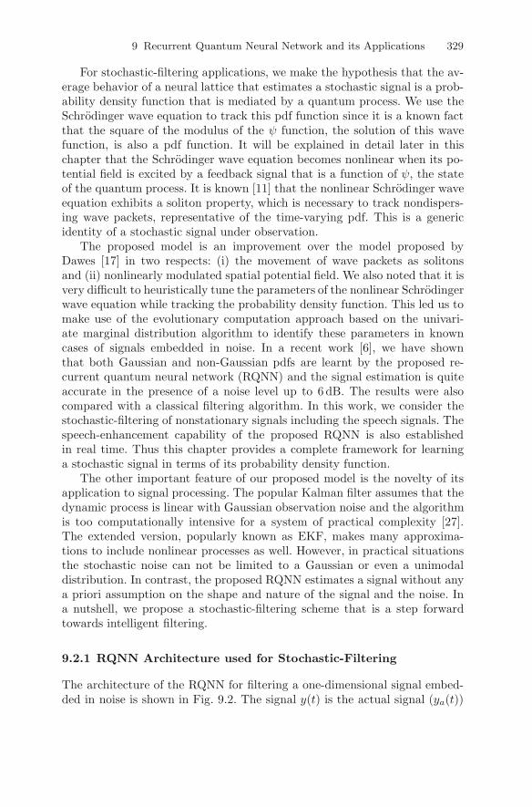
The architecture of the RQNN for filtering a one-dimensional signal embed-ded in noise is shown in Fig. 9.2. The signal y(t) is the actual signal (ya(t))
330 Laxmidhar Behera, Indrani Kar, and Avshalom C. Elitzur
y...
W1
WN
V (x)⊗1
N
Quantumactivationfunction(Schrodingerwave equation)
∫ψ∗xψdx
ψ
−
+ y
Fig. 9.2. A stochastic filter using RQNN with linear modulation
embedded in noise (µ(t)), i. e. y(t) = ya(t) + µ(t). The signal excites N neu-rons spatially located along the x-axis after being preprocessed by synapses.In the model the synapses are represented by time-varying synaptic weightsK(x, t). The unified dynamics of the one-dimensional neural lattice consistingof N neurons is described by the Schrodinger wave equation given as
i�∂ψ(x, t)
∂t= − �
2
2m∇2ψ(x, t) + ζ(U(x, t) + G(| ψ |2))ψ(x, t) , (9.1)
where i,�, ψ(x, t) and ∇ carry their usual meaning in the context of Schro-dinger wave equation. The ψ(x, t) function represents the solution of (9.1).The potential field of the Schrodinger wave equation given in (9.1) consistsof two terms:
U(x, t) = −K(x, t)y(t) , (9.2)
G(| ψ |2) = K(x, t)∫
xf(x, t)dx , (9.3)
wheref(x, t) =| ψ(x, t) |2 . (9.4)
Since the potential field term in (9.1) is a function of ψ(x, t), the Schrodingerwave equation that describes the stochastic filter is nonlinear. In contrast toartificial neural networks studied in the literature, in our model the neurallattice consisting of N neurons is described by the state ψ(x, t) which is thesolution of (9.1). Simultaneously, the model is recurrent as the dynamicsconsists of a feedback term G(.). The information about the signal is thustransferred to the potential field of the Schrodinger wave equation and thedynamics is evolved accordingly. Here we have used a linear neural circuit toset up the potential field where K(x, t)s are the associated linear synapticweights. The signal is then estimated using a maximum-likelihood estimatoras
y(t) =∫
xf(x, t)dx. (9.5)
9 Recurrent Quantum Neural Network and its Applications 331
When the estimate y(t) is the actual signal, then the signal that generatesthe potential field for the Schrodinger wave equation, ν(t), is simply the noisethat is embedded in the signal. If the statistical mean of the noise is zero,then this error-correcting signal ν(t) has little effect on the movement of thewave packet. Precisely, it is the actual signal content in the input y(t) thatmoves the wave packet along the desired direction that, in effect, achieves thegoal of the stochastic-filtering. It is expected that the synaptic weights evolvein such a manner so as to drive the ψ function to carry the exact informationof the pdf of the observed stochastic variable y(t).
Learning and Estimation
The nonlinear Schrodinger wave equation given by (9.1) exhibits a solitonproperty, i. e. the square of | ψ(x, t) | is a wave packet that moves like a parti-cle. The importance of this property is as follows. Let the stochastic variabley(t) be described by a Gaussian probability density function f(x, t) withmean κ and standard deviation σ. Let the initial state of (9.1) correspond tozero mean Gaussian probability density function f ′(x, t) with standard devi-ation σ′. As the dynamics evolves with online update of the synaptic weightsK(x, t), the probability density function f ′(x, t) should ideally move towardthe pdf, f(x) of the signal y(t). Thus the filtering problem in this new frame-work can be seen as the ability of the nonlinear Schrodinger wave equation toproduce a wave packet solution that glides along with the time-varying pdfcorresponding to the signal y(t).
The synaptic weights K(x, t), which is a N × 1-dimensional vector, isupdated using the Hebbian learning algorithm
∂K(x, t)∂t
= βν(t)f(x, t) , (9.6)
where ν(t) = y(t) − y(t). y(t) is the filtered estimate of the actual sig-nal ya(t). We compute the filtered estimate according to (9.5). We willshow later that the wave packet moves in the required direction in our newmodel.
9.2.2 Integration of the Schrodinger Wave Equation
The nonlinear Schrodinger wave equation is – from the mathematical pointof view – a partial differential equation with two variables: x and t. In anabstract sense, receptive fields of N neurons span the entire distance alongthe x-axis. (9.1) is converted into the finite difference form by dividing thex-axis into N mesh points so that x and t are represented as follows:
xj = j�x tn = n�t , (9.7)
332 Laxmidhar Behera, Indrani Kar, and Avshalom C. Elitzur
where j varies from −N/2 to +N/2. The finite-difference form of (9.1) isexpressed as
iψ(x, t + �t) − ψ(x, t)
�t=
− ψ(x + �x, t) − 2ψ(x, t) + ψ(x −�x, t)2m�x2 + V (x)ψ(x, t) , (9.8)
where V (x) = ζ(U(x, t) + G(| ψ |2)). Here, we have assumed that � = 1.For convenience, we represent ψ(xj , tn + �t) as ψj
n+1, ψ(xj , tn) as ψjn and
ψ(xj −�x, tn) as ψj−1n. With these representations, (9.8) reads
ψjn+1 = ψj
n + i�tψj+1
n − 2ψjn + ψj−1
n
2m�x2 − i�tVjψjn . (9.9)
Rewriting this equation in a matrix form one gets
Fn+1 = Fn − i�tH ′Fn , (9.10)
where the Hamiltonian H ′ is defined as
H ′ = − �2
2m
d2
dx2+ V (x) . (9.11)
Subsequently,Fn+1 = UFn where U = I − i�tH ′ . (9.12)
Since it is required that the norm of F is F ∗F = 1, U must be an orthonormaloperator. Since U in (9.12) does not have such a property, in our simulationwe impose the normalization after every step.
Selection of Parameters
The nonlinear equation (9.1) involves four external parameters: �, m, ζ andβ. The last parameter β is necessary to update the synaptic weight vectorK(x, t). For simplicity, the parameter � is taken as unity and the other threeparameters are tuned accordingly. Looking at the complexity of (9.1), we useda genetic algorithm (GA) based on the concept of the univariate marginaldistribution algorithm (UMDA) [5, 29] to select near-optimal parameters.The details of the algorithm and its implementation are as follows:
The univariate marginal distribution algorithm estimates the distributionof gene frequencies using a mean-field approximation. Each string in thepopulation is represented by a binary vector x. The algorithm generates newpoints according to the following distribution:
p(x, t) =n∏
i=1
psi (xi, t) . (9.13)

9 Recurrent Quantum Neural Network and its Applications 333
The UMDA algorithm is given as follows:
– Step 1: Set t = 1, Generate N(>> 0) binary strings randomly.– Step 2: Select M < N strings according to a selection method.– Step 3: Compute the marginal frequencies ps
i (xi, t) from the selectedstrings.
– Step 4: Generate N new points according to the distribution
p(x, t) =∏n
i=1 psi (xi, t) .
– Set t = t + 1. If the termination criteria are not met, go to Step 2.
For infinite populations and proportionate selection, it has been shown [29]that the average fitness never decreases for the maximization problem (in-creases for the minimization problem).
In general, GA provided the parameter values where m < 1, β < 1 andζ >> 1. The significance of this finding can be understood in the followingmanner. Since β was the learning parameter in the Hebbian learning, it isnatural to expect that β < 1. The less than unity value for m makes self-excitation larger. Similarly, a large value of ζ causes a larger input excitationsince it appears as a multiplicand in the Schrodinger equation.
9.2.3 Simulation Results I
The proposed RQNN has been successfully applied to denoising of various sig-nals like dc signals, sinusoids, shifted sinusoids, amplitude-modulated sine andsquare waves, speech signals, embedded in high Gaussian or non-Gaussiannoise. Some selected results are presented in this section.
Amplitude - Modulated Sine and Square Waves
Amplitude-modulated and frequency-modulated signals are normally used incoding and transmission of data and appear corrupted at the receiver’s endby channel noise [23]. For simulation purpose, we have selected the frequencyof the carrier signal to be a sinusoid of frequency 5 Hz, although in realitythey are very high frequency signals. The amplitude was modulated by su-perimposing a triangular variation of frequency 0.5Hz. Thus the expressionfor the composite signal ya(t) is
ya(t) = a(t) · sin(2π5t) ; a(t) ={
1.5t 0 ≤ t ≤ 11.5 (2 − t) 1 ≤ t ≤ 2 ,
(9.14)
where a(t) is periodic with period 0.5Hz. A similar strategy is applied ingenerating the amplitude modulated square wave, i. e., the amplitude of a(t)is kept constant over every single period of the carrier sine wave in (9.14).
334 Laxmidhar Behera, Indrani Kar, and Avshalom C. Elitzur
The expression for the actual signal ya(t) in this case is given below:
ya(t) ={
a(t) 0 ≤ t ≤ 0.1−a(t) 0.1 ≤ t ≤ 0.2 and a(t) =
{1.5t 0 ≤ t ≤ 11.5 (2 − t) 1 ≤ t ≤ 2 ,
(9.15)where a(t) is periodic with period 0.5Hz.
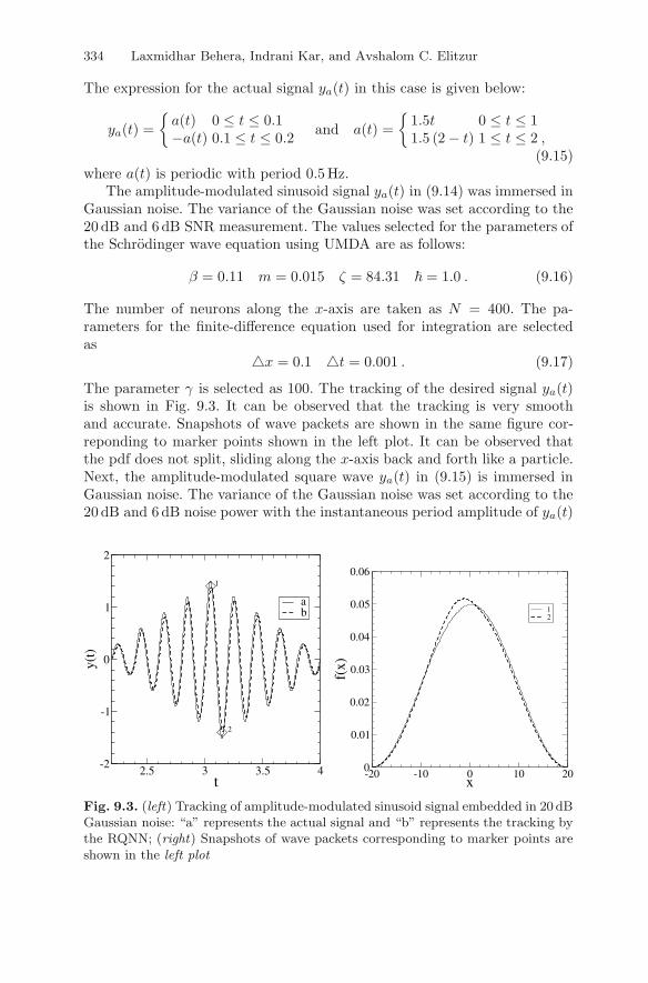
The amplitude-modulated sinusoid signal ya(t) in (9.14) was immersed inGaussian noise. The variance of the Gaussian noise was set according to the20 dB and 6dB SNR measurement. The values selected for the parameters ofthe Schrodinger wave equation using UMDA are as follows:
β = 0.11 m = 0.015 ζ = 84.31 � = 1.0 . (9.16)
The number of neurons along the x-axis are taken as N = 400. The pa-rameters for the finite-difference equation used for integration are selectedas
�x = 0.1 �t = 0.001 . (9.17)
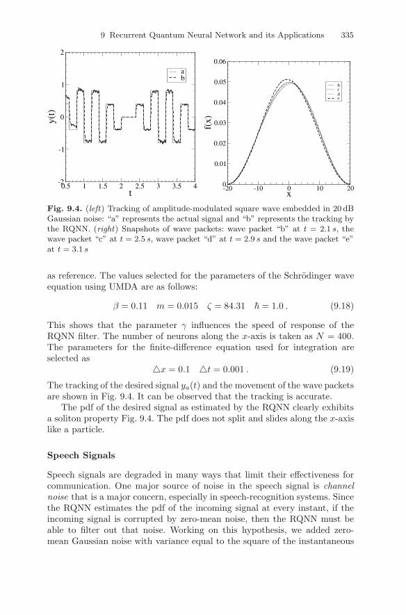
The parameter γ is selected as 100. The tracking of the desired signal ya(t)is shown in Fig. 9.3. It can be observed that the tracking is very smoothand accurate. Snapshots of wave packets are shown in the same figure cor-reponding to marker points shown in the left plot. It can be observed thatthe pdf does not split, sliding along the x-axis back and forth like a particle.Next, the amplitude-modulated square wave ya(t) in (9.15) is immersed inGaussian noise. The variance of the Gaussian noise was set according to the20 dB and 6 dB noise power with the instantaneous period amplitude of ya(t)
2.5 3 3.5 4t
-2
-1
0
1
2
y(t)
ab
1
2
-20 -10 0 10 20x
0
0.01
0.02
0.03
0.04
0.05
0.06
f(x)
12
Fig. 9.3. (left) Tracking of amplitude-modulated sinusoid signal embedded in 20 dBGaussian noise: “a” represents the actual signal and “b” represents the tracking bythe RQNN; (right) Snapshots of wave packets corresponding to marker points areshown in the left plot
9 Recurrent Quantum Neural Network and its Applications 335
0.5 1 1.5 2 2.5 3 3.5 4t
-2
-1
0
1
2y(
t)
ab
-20 -10 0 10 20x
0
0.01
0.02
0.03
0.04
0.05
0.06
f(x)
bcde
Fig. 9.4. (left) Tracking of amplitude-modulated square wave embedded in 20 dBGaussian noise: “a” represents the actual signal and “b” represents the tracking bythe RQNN. (right) Snapshots of wave packets: wave packet “b” at t = 2.1 s, thewave packet “c” at t = 2.5 s, wave packet “d” at t = 2.9 s and the wave packet “e”at t = 3.1 s
as reference. The values selected for the parameters of the Schrodinger waveequation using UMDA are as follows:
β = 0.11 m = 0.015 ζ = 84.31 � = 1.0 . (9.18)
This shows that the parameter γ influences the speed of response of theRQNN filter. The number of neurons along the x-axis is taken as N = 400.The parameters for the finite-difference equation used for integration areselected as
�x = 0.1 �t = 0.001 . (9.19)
The tracking of the desired signal ya(t) and the movement of the wave packetsare shown in Fig. 9.4. It can be observed that the tracking is accurate.
The pdf of the desired signal as estimated by the RQNN clearly exhibitsa soliton property Fig. 9.4. The pdf does not split and slides along the x-axislike a particle.
Speech Signals
Speech signals are degraded in many ways that limit their effectiveness forcommunication. One major source of noise in the speech signal is channelnoise that is a major concern, especially in speech-recognition systems. Sincethe RQNN estimates the pdf of the incoming signal at every instant, if theincoming signal is corrupted by zero-mean noise, then the RQNN must beable to filter out that noise. Working on this hypothesis, we added zero-mean Gaussian noise with variance equal to the square of the instantaneous
336 Laxmidhar Behera, Indrani Kar, and Avshalom C. Elitzur
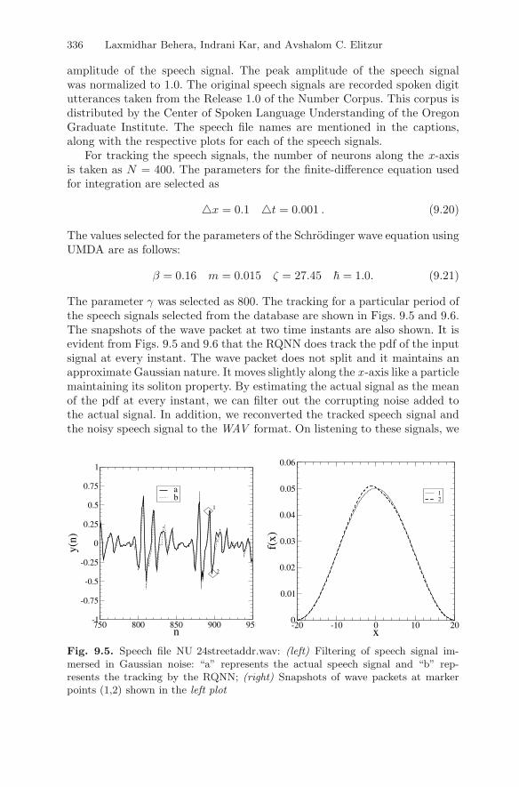
amplitude of the speech signal. The peak amplitude of the speech signalwas normalized to 1.0. The original speech signals are recorded spoken digitutterances taken from the Release 1.0 of the Number Corpus. This corpus isdistributed by the Center of Spoken Language Understanding of the OregonGraduate Institute. The speech file names are mentioned in the captions,along with the respective plots for each of the speech signals.
For tracking the speech signals, the number of neurons along the x-axisis taken as N = 400. The parameters for the finite-difference equation usedfor integration are selected as
�x = 0.1 �t = 0.001 . (9.20)
The values selected for the parameters of the Schrodinger wave equation usingUMDA are as follows:
β = 0.16 m = 0.015 ζ = 27.45 � = 1.0. (9.21)
The parameter γ was selected as 800. The tracking for a particular period ofthe speech signals selected from the database are shown in Figs. 9.5 and 9.6.The snapshots of the wave packet at two time instants are also shown. It isevident from Figs. 9.5 and 9.6 that the RQNN does track the pdf of the inputsignal at every instant. The wave packet does not split and it maintains anapproximate Gaussian nature. It moves slightly along the x -axis like a particlemaintaining its soliton property. By estimating the actual signal as the meanof the pdf at every instant, we can filter out the corrupting noise added tothe actual signal. In addition, we reconverted the tracked speech signal andthe noisy speech signal to the WAV format. On listening to these signals, we
750 800 850 900 950n
-1
-0.75
-0.5
-0.25
0
0.25
0.5
0.75
1
y(n)
ab
1
2
-20 -10 0 10 20x
0
0.01
0.02
0.03
0.04
0.05
0.06
f(x)
12
Fig. 9.5. Speech file NU 24streetaddr.wav: (left) Filtering of speech signal im-mersed in Gaussian noise: “a” represents the actual speech signal and “b” rep-resents the tracking by the RQNN; (right) Snapshots of wave packets at markerpoints (1,2) shown in the left plot
9 Recurrent Quantum Neural Network and its Applications 337
1200 1250 1300 1350 1400n
-1
-0.75
-0.5
-0.25
0
0.25
0.5
0.75
1y(
n)
ab
-20 -10 0 10 20x
0
0.01
0.02
0.03
0.04
0.05
0.06
f(x)
bd
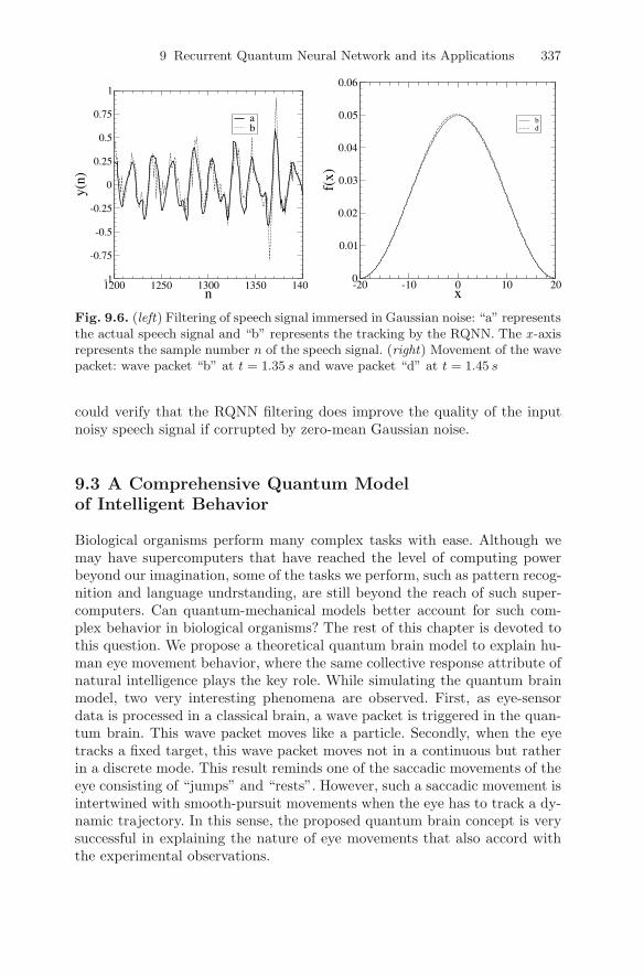
Fig. 9.6. (left) Filtering of speech signal immersed in Gaussian noise: “a” representsthe actual speech signal and “b” represents the tracking by the RQNN. The x -axisrepresents the sample number n of the speech signal. (right) Movement of the wavepacket: wave packet “b” at t = 1.35 s and wave packet “d” at t = 1.45 s
could verify that the RQNN filtering does improve the quality of the inputnoisy speech signal if corrupted by zero-mean Gaussian noise.
9.3 A Comprehensive Quantum Modelof Intelligent Behavior
Biological organisms perform many complex tasks with ease. Although wemay have supercomputers that have reached the level of computing powerbeyond our imagination, some of the tasks we perform, such as pattern recog-nition and language undrstanding, are still beyond the reach of such super-computers. Can quantum-mechanical models better account for such com-plex behavior in biological organisms? The rest of this chapter is devoted tothis question. We propose a theoretical quantum brain model to explain hu-man eye movement behavior, where the same collective response attribute ofnatural intelligence plays the key role. While simulating the quantum brainmodel, two very interesting phenomena are observed. First, as eye-sensordata is processed in a classical brain, a wave packet is triggered in the quan-tum brain. This wave packet moves like a particle. Secondly, when the eyetracks a fixed target, this wave packet moves not in a continuous but ratherin a discrete mode. This result reminds one of the saccadic movements of theeye consisting of “jumps” and “rests”. However, such a saccadic movement isintertwined with smooth-pursuit movements when the eye has to track a dy-namic trajectory. In this sense, the proposed quantum brain concept is verysuccessful in explaining the nature of eye movements that also accord withthe experimental observations.

338 Laxmidhar Behera, Indrani Kar, and Avshalom C. Elitzur
9.4 RQNN-based Eye-Tracking Model
There are certain aspects of brain functions that still appear to have nosatisfactory explanation. As an alternative, researchers [36, 37, 21, 28] are in-vestigating whether the brain can demonstrate quantum-mechanical behav-ior. According to a current hypothesis, microtubules, the basic components ofneural cytoskeleton, are very likely to possess quantum-mechanical propertiesdue to their size and structure. The tubulin protein, which is the structuralblock of microtubules, has the ability to flip from one conformation to anotheras a result of a shift in the electron-density localization from one resonanceorbital to another. These two conformations act as two basis states of thesystem according to whether the electrons inside the tubuline hydrophobicpocket are localized closer to α or β tubulin. Moreover, the system can lie ina superposition of these two basis states, that is, being in both states simul-taneously, which can give a plausible mechanism for creating a coherent statein the brain. Penrose [30] therefore argued that the human brain must utilizequantum-mechanical effects when demonstrating problem solving feats thatcannot be explained algorithmically.
In this chapter, instead of going into the biological details of the brain,we propose a theoretical quantum brain model using the RQNN. The RQNNmodel proposed in Sect. 9.2.1 has been modified a little to cope with thepresent application. Instead of using a linear neural circuit to set up the po-tential field in which the quantum brain is dynamically excited, the presentmodel uses a nonlinear neural circuit. This fundamental change in the archi-tecture has yielded two novel features. The wave packets, f(x, t) =| ψ(x, t) |2,are moving like particles. Here ψ(x, t) is the solution of the nonlinearSchrodinger wave equation that describes the proposed quantum brain modelto explain eye movements for tracking moving targets. The other very inter-esting observation is that the movements of the wave packets, while trackinga fixed target, are not continuous but discrete. These observations accord withthe well-known saccadic movement of the eye [3, 18]. In a way, our model isthe first of its kind to explain the nature of eye movements in static scenesthat consists of “jumps” (saccades) and “rests” (fixations). We expect thisresult to inspire other researchers to further investigate the possible quantumdynamics of the brain.
9.4.1 A Theoretical Quantum Brain Model
An impetus to hypothesize a quantum brain model comes from the brain’snecessity to unify the neuronal response into a single percept. Anatomical,neurophysiological and neuropsychological evidences, as well as brain imagingusing fMRI and PET scans, show that separate functional MAPs exist in thebrain to code separate features such as direction of motion, location, colorand orientation. How does the brain compute all these data to have a coherentperception? Here, a very simple model of a quantum brain is proposed, where
9 Recurrent Quantum Neural Network and its Applications 339
.
.
ψ1
ψ2
ψN
Neural Lattice
A single
stimulus
ψ = c1ψ1 + c2ψ2 + .. + cNψN
Collective Response
Fig. 9.7. Quantum brain – a theoretical model
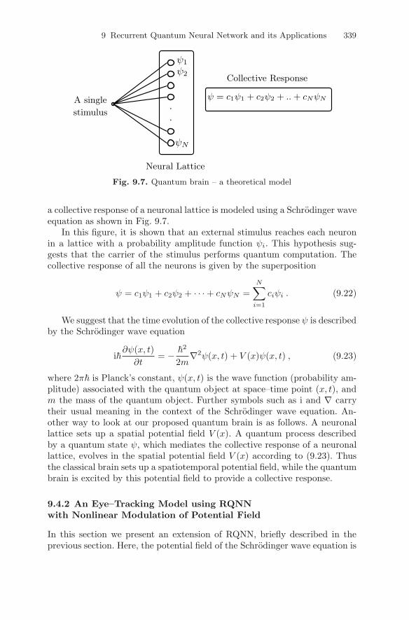
a collective response of a neuronal lattice is modeled using a Schrodinger waveequation as shown in Fig. 9.7.
In this figure, it is shown that an external stimulus reaches each neuronin a lattice with a probability amplitude function ψi. This hypothesis sug-gests that the carrier of the stimulus performs quantum computation. Thecollective response of all the neurons is given by the superposition
ψ = c1ψ1 + c2ψ2 + · · · + cNψN =N∑
i=1
ciψi . (9.22)
We suggest that the time evolution of the collective response ψ is describedby the Schrodinger wave equation
i�∂ψ(x, t)
∂t= − �
2
2m∇2ψ(x, t) + V (x)ψ(x, t) , (9.23)
where 2π� is Planck’s constant, ψ(x, t) is the wave function (probability am-plitude) associated with the quantum object at space–time point (x, t), andm the mass of the quantum object. Further symbols such as i and ∇ carrytheir usual meaning in the context of the Schrodinger wave equation. An-other way to look at our proposed quantum brain is as follows. A neuronallattice sets up a spatial potential field V (x). A quantum process describedby a quantum state ψ, which mediates the collective response of a neuronallattice, evolves in the spatial potential field V (x) according to (9.23). Thusthe classical brain sets up a spatiotemporal potential field, while the quantumbrain is excited by this potential field to provide a collective response.
9.4.2 An Eye–Tracking Model using RQNNwith Nonlinear Modulation of Potential Field
In this section we present an extension of RQNN, briefly described in theprevious section. Here, the potential field of the Schrodinger wave equation is
340 Laxmidhar Behera, Indrani Kar, and Avshalom C. Elitzur
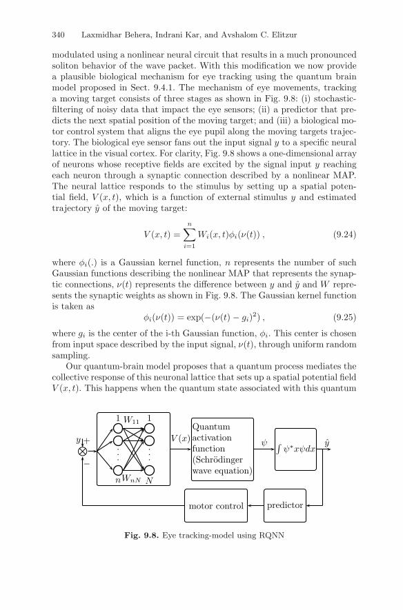
modulated using a nonlinear neural circuit that results in a much pronouncedsoliton behavior of the wave packet. With this modification we now providea plausible biological mechanism for eye tracking using the quantum brainmodel proposed in Sect. 9.4.1. The mechanism of eye movements, trackinga moving target consists of three stages as shown in Fig. 9.8: (i) stochastic-filtering of noisy data that impact the eye sensors; (ii) a predictor that pre-dicts the next spatial position of the moving target; and (iii) a biological mo-tor control system that aligns the eye pupil along the moving targets trajec-tory. The biological eye sensor fans out the input signal y to a specific neurallattice in the visual cortex. For clarity, Fig. 9.8 shows a one-dimensional arrayof neurons whose receptive fields are excited by the signal input y reachingeach neuron through a synaptic connection described by a nonlinear MAP.The neural lattice responds to the stimulus by setting up a spatial poten-tial field, V (x, t), which is a function of external stimulus y and estimatedtrajectory y of the moving target:
V (x, t) =n∑
i=1
Wi(x, t)φi(ν(t)) , (9.24)
where φi(.) is a Gaussian kernel function, n represents the number of suchGaussian functions describing the nonlinear MAP that represents the synap-tic connections, ν(t) represents the difference between y and y and W repre-sents the synaptic weights as shown in Fig. 9.8. The Gaussian kernel functionis taken as
φi(ν(t)) = exp(−(ν(t) − gi)2) , (9.25)
where gi is the center of the i-th Gaussian function, φi. This center is chosenfrom input space described by the input signal, ν(t), through uniform randomsampling.
Our quantum-brain model proposes that a quantum process mediates thecollective response of this neuronal lattice that sets up a spatial potential fieldV (x, t). This happens when the quantum state associated with this quantum
y
1 1W11
WnNn N
V (x)..
⊗.
.
.
.
motor control predictor
Quantumactivationfunction(Schrodingerwave equation)
∫ψ∗xψdx
ψ
−
+ y
Fig. 9.8. Eye tracking-model using RQNN
9 Recurrent Quantum Neural Network and its Applications 341
process evolves in this potential field. The spatiotemporal evolution follows asper (9.23). We hypothesize that this collective response is described by a wavepacket, f(x, t) =| ψ(x, t) |2, where the term ψ(x, t) represents a quantumstate. In a generic sense, we assume that a classical stimulus in a brain triggersa wave packet in the counterpart “quantum brain”. This subjective response,f(x, t), is quantified using the following estimate equation:
y(t) =∫
x(t)f(x, t)dx . (9.26)
The estimate equation is motivated by the fact that the wave packet,f(x, t) =| ψ(x, t) |2 is interpreted as the probability density function. Al-though computation of (9.26) using the nonlinear Schrodinger wave equationis straightforward, we hypothesize that this computation can be done throughan interaction between a quantum and a classical brain, using a suitablequantum measurement operator. At this point we will not speculate aboutthe nature of such a quantum measurement operator that will estimate theψ function necessary to compute (9.26). Based on this estimate, y, the pre-dictor estimates the next spatial position of the moving target. To simplifyour analysis, the predictor is made silent. Thus its output is the same as thatof y. The biological motor control is commanded to fixate the eye pupil toalign with the target position, which is predicted to be at y. Obviously, wehave assumed that biological motor control is ideal.
After the above-mentioned simplification, the closed form dynamics of themodel described by Fig. 9.8 becomes
i�∂ψ(x, t)
∂t= − �
2
2m∇2ψ(x, t) + ζG
(y(t) −
∫x | ψ(x, t) |2 dx
), ψ(x, t) ,
(9.27)where G(.) is a Gaussian kernel MAP introduced to nonlinearly modulatethe spatial potential field that excites the dynamics of the quantum object.In fact, ζG(.) = V (x, t), where V (x, t) is given in (9.24).
The nonlinear Schrodinger wave equation given by (9.27) is one-di-mensional with cubic nonlinearity. Interestingly, the closed-form dynamicsof the recurrent quantum neural network (equation (9.27)) closely resemblesa nonlinear Schrodinger wave equation with cubic nonlinearity studied inquantum electrodynamics [20]:
i�∂ψ(x, t)
∂t=(− �
2
2m∇2 − e2
r
)ψ(x, t) + e2
∫ψ(x, t) | ψ(x′, t) |2
| x − x′ | dx′ ,
(9.28)where m is the electron mass, e the elementary charge and r the magnitudeof | x |. Also, nonlinear Schrodinger wave equations with cubic nonlinearityof the form ∂
∂tA(t) = c1A + c3 | A |2 A, where c1 and c3 are constants,frequently appear in nonlinear optics [12] and in the study of solitons [24, 11,15, 33]. Application of the nonlinear Schrodinger wave equation for the studyof quantum systems can also be found in [34].
342 Laxmidhar Behera, Indrani Kar, and Avshalom C. Elitzur
In (9.27), the unknown parameters are weights Wi(x, t) associated withthe Gaussian kernel, mass m, and ζ, the scaling factor to actuate the spatialpotential field. The weights are updated using the Hebbian learning algorithm
∂Wi(x, t)∂t
= βφi(ν(t))f(x, t) , (9.29)
where ν(t) = y(t) − y(t).The idea behind the proposed quantum computing model is as follows. As
an individual observes a moving target, the uncertian spatial position of themoving target triggers a wave packet within the quantum brain. The quantumbrain is so hypothesized that this wave packet turns out to be a collectiveresponse of a classical neural lattice. As we combine (9.27) and (9.29), it isdesired that there exist some parameters m, ζ and β such that each specificspatial position x(t) triggers a unique wave packet, f(x, t) =| ψ(x, t) |2, inthe quantum brain. This brings us to the question of whether the closedform dynamics can exhibit soliton properties that are desirable for targettracking. As pointed out above, our equation has a form that is known topossess soliton properties for a certain range of parameters and we just haveto find those parameters for each specific problem.
We would like to reiterate the importance of the soliton properties. Ac-cording to our model, eye tracking means tracking of a wave packet in thedomain of the quantum brain. The biological motor control aligns the eyepupil along the spatial position of the external target that the eye tracks. Asthe eye sensor receives data y from this position, the resulting error stimulatesthe quantum brain. In a noisy background, if the tracking is accurate, thenthis error-correcting signal ν(t) has little effect on the movement of the wavepacket. Precisely, it is the actual signal content in the input y(t) that movesthe wave packet along the desired direction that, in effect, achieves the goalof the stochastic filtering part of the eye movement for tracking purposes.
9.4.3 Simulation Results II
In this section we present simulation results to test target tracking througheye movement where targets are either fixed or moving.
For fixed target tracking, we have simulated a stochastic-filtering problemof a dc signal embedded in Gaussian noise. As the eye tracks a fixed target,the corresponding dc signal is taken as ya(t) = 2.0, embedded in Gaussiannoise with SNR (signal-to-noise ratio) values of 20 dB, 6 dB and 0 dB.
We next compared the results with the performance of a Kalman fil-ter [19] designed for this purpose. It should be noted that the operation ofthe Kalman filter is based on a priori information that the embedded signalis a dc signal, whereas the RQNN is not provided with this information. TheKalman filter also makes use of the fact that the noise is Gaussian and esti-mates the variance of the noise based on this assumption. Thus it is expected
9 Recurrent Quantum Neural Network and its Applications 343
that the performance of the Kalman filter will degrade as the noise becomesnon-Gaussian. In contrast, the RQNN model does not make any assumptionabout the noise.
Notice that there are certain values of β, m, ζ and N for which the modelperforms optimally. A univariate marginal distribution algorithm was used toget near optimal parameters while fixing N = 400 and � = 1.0. The selectedvalues of these parameters are as follows for all levels of SNR:
β = 0.86; m = 2.5; ζ = 2000. (9.30)
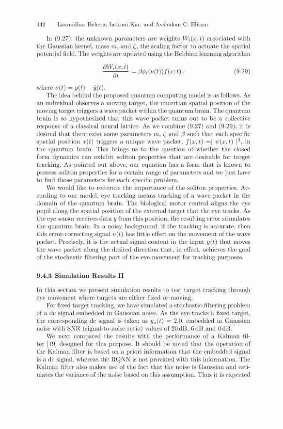
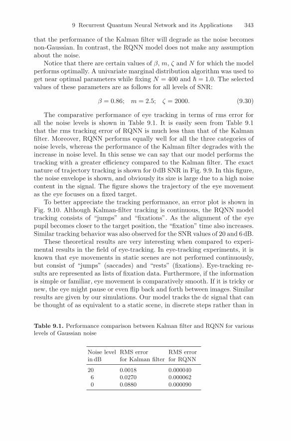
The comparative performance of eye tracking in terms of rms error forall the noise levels is shown in Table 9.1. It is easily seen from Table 9.1that the rms tracking error of RQNN is much less than that of the Kalmanfilter. Moreover, RQNN performs equally well for all the three categories ofnoise levels, whereas the performance of the Kalman filter degrades with theincrease in noise level. In this sense we can say that our model performs thetracking with a greater efficiency compared to the Kalman filter. The exactnature of trajectory tracking is shown for 0 dB SNR in Fig. 9.9. In this figure,the noise envelope is shown, and obviously its size is large due to a high noisecontent in the signal. The figure shows the trajectory of the eye movementas the eye focuses on a fixed target.
To better appreciate the tracking performance, an error plot is shown inFig. 9.10. Although Kalman-filter tracking is continuous, the RQNN modeltracking consists of “jumps” and “fixations”. As the alignment of the eyepupil becomes closer to the target position, the “fixation” time also increases.Similar tracking behavior was also observed for the SNR values of 20 and 6 dB.
These theoretical results are very interesting when compared to experi-mental results in the field of eye-tracking. In eye-tracking experiments, it isknown that eye movements in static scenes are not performed continuously,but consist of “jumps” (saccades) and “rests” (fixations). Eye-tracking re-sults are represented as lists of fixation data. Furthermore, if the informationis simple or familiar, eye movement is comparatively smooth. If it is tricky ornew, the eye might pause or even flip back and forth between images. Similarresults are given by our simulations. Our model tracks the dc signal that canbe thought of as equivalent to a static scene, in discrete steps rather than in
Table 9.1. Performance comparison between Kalman filter and RQNN for variouslevels of Gaussian noise
Noise level RMS error RMS errorin dB for Kalman filter for RQNN
20 0.0018 0.0000406 0.0270 0.0000620 0.0880 0.000090
344 Laxmidhar Behera, Indrani Kar, and Avshalom C. Elitzur
0 1 2 3 4t
-6
-4
-2
0
2
4
6
8
10y a(t
)
abcd
1
2
3
-3 -2 -1 0 1 2 3x
0
2
4
6
8
10
f(x)
123
Initial
Fig. 9.9. (left) Eye tracking of a fixed target in a noisy environment of 0 dB SNR:“a” respresents fixed target, “b” represents target tracking using RQNN modeland “c” represents target tracking using a Kalman filter. The noise envelope isrepresented by the curve “d”; (right) The snapshots of the wave packets at differentinstances corresponding to the marker points (1,2,3) as shown in the left figure.The solid line represent the initial wave packet assigned to the Schrodinger waveequation
a continuous fashion. This is very clearly understood from the tracking errorin Fig. 9.10.
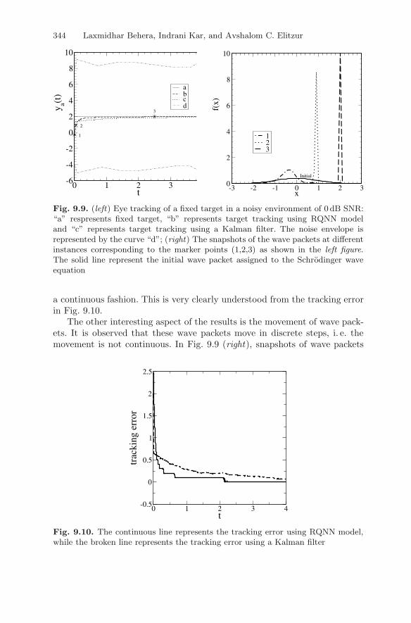
The other interesting aspect of the results is the movement of wave pack-ets. It is observed that these wave packets move in discrete steps, i. e. themovement is not continuous. In Fig. 9.9 (right), snapshots of wave packets
0 1 2 3 4t
-0.5
0
0.5
1
1.5
2
2.5
trac
king
err
or
Fig. 9.10. The continuous line represents the tracking error using RQNN model,while the broken line represents the tracking error using a Kalman filter
9 Recurrent Quantum Neural Network and its Applications 345
-20 -10 0 10 20x
0
0.1
0.2
0.3
0.4
f(x)
123
Initial Wave Packet
Fig. 9.11. Wave-packet movements for RQNN with linear weights
are plotted at different instances corresponding to marker points as shownalong the desired trajectory. It can be noticed that a very flat initial Gaussianwave packet first moves to the left, and then proceeds toward the right un-til the mean of the wave packet exactly matches the actual spatial position.A similar pattern of movement of wave packets was also noticed in the caseof 20 and 6 dB SNR. The wave-packet movement is compared with the same,when instead of nonlinear modulation of the potential field, we use a linearmodulation as described in Sect. 9.2.1 in Fig. 9.11. The initial wave packetin the previous model first splits into two parts, then moves in a continuousfashion, ultimately going into a state with a mean of approximately 2 butwith high variance. In contrast, in the present model there is no splittingof the wave packet, movement is discrete and variance is also much smaller.Thus the soliton behavior of the present model is highly pronounced.
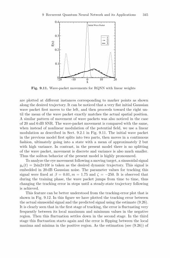
To analyze the eye movement following a moving target, a sinusoidal signalya(t) = 2sin2π10t is taken as the desired dynamic trajectory. This signal isembedded in 20 dB Gaussian noise. The parameter values for tracking thissignal were fixed at β = 0.01, m = 1.75 and ζ = −250. It is observed thatduring the training phase, the wave packet jumps from time to time, thuschanging the tracking error in steps until a steady-state trajectory followingis achieved.
This feature can be better understood from the tracking-error plot that isshown in Fig. 9.12. In this figure we have plotted the tracking error betweenthe actual sinusoidal signal and the predicted signal using the estimate (9.26).It is clearly seen that in the first stage of tracking, the error is fluctuating veryfrequently between its local maximum and minimum values in the negativeregion. Then this fluctuation settles down in the second stage. In the thirdstage this fluctuation starts again and the error is flipping between the localmaxima and minima in the positive region. As the estimation (see (9.26)) of

346 Laxmidhar Behera, Indrani Kar, and Avshalom C. Elitzur
0 2 4 6 8 10t
-4
-2
0
2
4
6
8
trac
king
err
or
Fig. 9.12. Saccadic and pursuit movement of eye during dynamic trajectory fol-lowing
the signal is very much dependent on the nature of the wave packet, the errordynamics is also correlated with the wave-packet movement. Discontinuties inerror are reflected in the movement of the wave packet. It is obvious that theposition of the wave packet is changing very frequently in the first stage, thuschanging the mean value correspondingly, and it has no connection with thesignal mean value. This means that there are a number of discontinuties or“jumps” in the wave-packet movement in the first stage. Then, in the secondstage the movement becomes continuous with the mean values following thesignal mean values. Again in the third stage the discontinuties take placeseveral times, ultimately achieving a steady-state movement in the last stage.
Once a steady state is achieved, the tracking is efficient and the wave-packet movement is continuous, as shown in Fig. 9.13. In this figure, thesnapshots of wave packets are plotted for three different instances of timeindicated by the marker points (1,2,3) as shown in the trajectory tracking.When the signal is at position 1, the corresponding wave packet has a mean at0. When the signal is at position 2, the corresponding wave packet has a meanat +2, and the mean of the wave packet moves to –2 when the signal goes toposition 3. As seen in Fig. 9.13, during the continuous movement of the wavepackets, trajectory tracking is smooth, which is similar to smooth-pursuitmovement of biological eye tracking. Smooth pursuit is the eye movementthat smoothly tracks slowly moving targets in the visual field. The purpose ofsmooth pursuit is partly to stabilize moving targets on the retina. It is a muchslower movement than saccades. Eye-tracking experiments reveal that whenpursuing a moving target, the smooth eye movements generally have a gainless than unity. The errors introduced by this are corrected by saccades thatbring the target back on the fovea. Thus after one or two quick saccadesto capture the target, the eye movement attains a steady-state velocity that
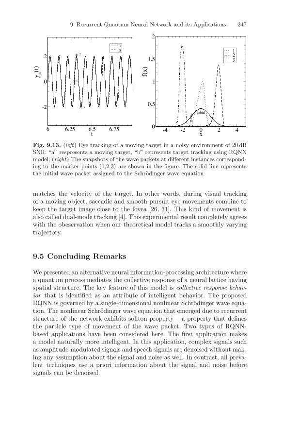
9 Recurrent Quantum Neural Network and its Applications 347
6 6.25 6.5 6.75 7t
-2
0
2
y a(t)
ab
1
2
3
-4 -2 0 2 4x
0
0.5
1
1.5
2
f(x)
123
Initial
Fig. 9.13. (left) Eye tracking of a moving target in a noisy environment of 20 dBSNR: “a” respresents a moving target, “b” represents target tracking using RQNNmodel; (right) The snapshots of the wave packets at different instances correspond-ing to the marker points (1,2,3) are shown in the figure. The solid line representsthe initial wave packet assigned to the Schrodinger wave equation
matches the velocity of the target. In other words, during visual trackingof a moving object, saccadic and smooth-pursuit eye movements combine tokeep the target image close to the fovea [26, 31]. This kind of movement isalso called dual-mode tracking [4]. This experimental result completely agreeswith the obeservation when our theoretical model tracks a smoothly varyingtrajectory.
9.5 Concluding Remarks
We presented an alternative neural information-processing architecture wherea quantum process mediates the collective response of a neural lattice havingspatial structure. The key feature of this model is collective response behav-ior that is identified as an attribute of intelligent behavior. The proposedRQNN is governed by a single-dimensional nonlinear Schrodinger wave equa-tion. The nonlinear Schrodinger wave equation that emerged due to recurrentstructure of the network exhibits soliton property – a property that definesthe particle type of movement of the wave packet. Two types of RQNN-based applications have been considered here. The first application makesa model naturally more intelligent. In this application, complex signals suchas amplitude-modulated signals and speech signals are denoised without mak-ing any assumption about the signal and noise as well. In contrast, all preva-lent techniques use a priori information about the signal and noise beforesignals can be denoised.

348 Laxmidhar Behera, Indrani Kar, and Avshalom C. Elitzur
The second application is a quantum brain model of eye tracking. Thekey concept here is that quantum-based models can be more predictive toexplain complex biological phenomena such as eye-movement behavior. Theinteresting finding is that our theoretical model of eye tracking agrees withpreviously observed experimental results. The model predicts that eye move-ments will be of saccadic type while following a static trajectory. In the caseof a dynamic trajectory, the eye movement consists of saccades and smoothpursuits. In this sense, the proposed quantum brain concept is very success-ful in explaining the nature of eye movements. Earlier explanations [3] forsaccadic movement have been primarily attributed to a motor control mech-anism, whereas the present model emphasizes that such eye movements aredue to a decision-making process of the brain – albeit a quantum brain.Thus the contribution of this chapter for the explanation of biological eyemovement as a neural information-processing event may inspire researchersto study quantum brain models from the biological perspective.
The other significant contribution is the prediction efficiency of the pro-posed model over the prevailing model. The stochastic-filtering of a dc signalusing RQNN is 1000 times more accurate compared to a Kalman filter.
At this point we are silent about the exact biological connection betweenthe classical and the quantum brain, as it is not clear to us. The model justassumes that the quantum brain is excited by the potential field set up bythe classical brain. Another obvious question is that of decoherence. In thisregard, we admit that the model proposed here is highly idealized since wehave used the Schrodinger wave equation. In our future work we intend toreplace the Schrodinger wave equation by a density matrix approach. Also,the phase-transition analysis of closed form dynamics, given in (9.27) withrespect to various parameters m, ζ, β and N , has been kept for future work.
Finally, we believe that apart from the computational power derived fromquantum computing, quantum learning systems may also provide a potentframework to study the subjective aspects of the nervous system [22]. Thechallenge to bridge the gap between physical and mental (or objective andsubjective) aspects of matter may be most successfully met within the frame-work of quantum learning systems. In this framework, we have proposed a no-tion of a quantum brain, and a recurrent quantum neural network has beenhypothesized as a first step towards a neural computing model.
References
1. Amari, S. (1983). IEEE Trans SMC, SMC-13(5):741–748.2. Amit, D.J. (1989). Modeling Brain Function. Springer-Verlag, Berlin/Heidel-
berg.3. Bahill, A.T. and Stark, L. (1979). Scientific American 240:84–93.4. Bahill, A.T., Iandolo, M.J., and Troost, B.T. (1980). Vision Research,
20:923–931.
9 Recurrent Quantum Neural Network and its Applications 349
5. Behera, L. (2002). New Optimization Techniques in Engineering, chapterParametric Optimization of a Fuzzy Logic Controller for Nonlinear DynamicalSystems using Evolutionary Computation. McGraw-Hill. New York.
6. Behera, L. and Sundaram, B. (2004). Proceedings, International Conferenceon Intelligent Sensors and Information Processing.
7. Behera, L., Gopal, M., and Chaudhury, S. (1996). IEEE Trans Neural Net-works, 7(6):1401–1414.
8. Behera, L., Chaudhury, S., and Gopal, M. (1998). IEE Proceedings ControlTheory and Applications, 145(2):134–140.
9. Behrman, E.C., Chandrashekar, V., Wang, Z., Belur, C.K., Steck, J.E., andSkinner, S.R. (2002). Physical Review Letters. Submitted.
10. Behrman, E.C., Nash, L.R., Steck, J.E., Chandrashekar, V.G., and Skin-ner, S.R. (2000). Information Sciences, 128(3–4):257–269.
11. Bialynicki-Birula, I. and Mycielski, J. (1976). Annals of Physics, 100:62–93.12. Boyd, R.W. (1991). Nonlinear Optics. Academic Press. London.13. Bucy, R.S. (1970). IEEE Proceedings, 58(6):854–864.14. Cohen, M.A. and Grossberg, S. (1983). IEEE Trans Syst, Man and Cybernet-
ics, 13:815–826.15. Davydov, A.S. (1982). Biology and Quantum Mechanics. Pergamon Press,
Oxford.16. Dawes, R.L. (1992). IJCNN Proceedings, 133.17. Dawes, R.L. (1993). Rethinking Neural Networks: Quantum Fields and Bio-
logical Data, chapter – Advances in the theory of quantum neurodynamics.Erlbaum, Hillsdale, N.J.
18. Findlay, J.M. Brown, V., and Gilchrist, I.D. (2001). Vision Research,41:87–95.
19. Grewal, M.S. and Andrews, A.P. (2001). Kalman Filtering: Theory and Prac-tice Using MATLAB. Wiley-Interscience. USA.
20. Gupta, S. and Zia, R.K.P. (2001). Journal of Computer and System Sciences,63(3):355–383.
21. Hagan, S., Hameroff, S.R., and Tuszynski, J.A. (2002). Physical Review E,65:061901.
22. Atmanspacher, H. (2004). Discrete Dynamics, 8:51–73.23. Haykin, S. (2001). Communication Systems. John Wiley and Sons, Inc., 4th
edn. New York.24. Jackson, E. Atlee (1991). Perspectives of Nonlinear Dynamics. Cambridge.
Cambridge University Press.25. Kennedy, J. and Eberhart, R.C. (2001). Swarm Intelligence. Morgan
Kauffman. USA.26. Leung, H. and Kettner, R.E. (1997). Vision Research, 37(10):1347–1354.27. Mendel, J.M. (1971). IEEE Trans Automatic Control, AC-16:748–758.28. Mershin, A., Nanopoulos, D.V., and Skoulakis, E. (1999). Proc. Acad. Athens,
74:148–179.29. Muehlenbein, H. and Thilo Mahnig. (2001). Foundations of Real-World Intel-
ligence, chapter – Evolutionary Computation and Beyond. CSLI Publications.Stanford.
30. Penrose, R. (1994). Shadows of the Mind. Oxford University Press. Oxford.31. Pola, J., and Wyatt, H.J. (1997). Vision Research, 37(18):2579–2595.

350 Laxmidhar Behera, Indrani Kar, and Avshalom C. Elitzur
32. Purushothaman, G. and Karayiannis, N.B. (1997). IEEE Tran. on NeuralNetworks, 8(3):679–693.
33. Scott, A.C., Chu, F.Y.F., and McLaughlin, D.W. (1973). IEEE Proceedings,61(10):1443–1483.
34. Sulem, C., Sulem, P.L., and Sulem, C. (1999). Nonlinear Schrodinger Equa-tions: Self-Focusing and Wave Collapse. Springer-Verlag. (Applied Mathemat-ical Sciences/139). New York.
35. Turing, A.M. (1950). Mind, 59:433–460.36. Tuszynski, J.A., Hameroff, S.R., Sataric, M.V., Trpisova, B., and Nip, M.L.A.
(1995). Journal of Theoretical Biology, 174:371–380.37. Vitiello, G. (1995). International Journal of Modern Physics B, 9:973–989.