9 isotope distributions and isotope patterns draft · draft 9 isotope distributions and isotope...

DRAFT

9 Isotope Distributions and Isotope

Patterns

“Two very significant discoveries are due to mass spectroscopic studies. First,J.J. Thomson discovered that neon consisted of a mixture of two different isotopes(masses 20 and 22) rather than only a single isotope. This observation of the exis-tence of stable isotopes is perhaps the greatest achievement that can be claimed bymass spectroscopy. [. . . ] The second significant discovery due to mass spectrographicstudies was made by F.W. Aston. He observed that the masses of all isotopes are notsimple multiples of a fundamental unit, but rather they are characterized by a massdefect; i.e., isotopes do not have integral masses.” (Robert W. Kiser, The Introductionto Mass Spectrometry)

MASS spectrometry cannot detect single molecules, but is dependent on the existence ofmillions of “identical” copies of some molecule. These copies are identical from a chemical

standpoint, but not from a physical standpoint: Throughout these copies, elements follow theirnatural isotope abundances. For mass spectrometry, this implies that instead of a single peak,we observe an isotope pattern of the molecule. On the one hand, this is simply an additionalcomplication that we have to deal with when analyzing MS data. In many MS applications,the experimental setup is actually chosen so that we do not have to consider such isotopepatterns: In peptide de novo sequencing introduced in Chapter 2, one deliberately selects onlythe monoisotopic peak (see below) for fragmentation, and no isotope patterns can be observed inthe fragmentation spectrum. On the other hand, we can use this fact to our advantage: Namely,we can use the isotope pattern to derive information about an unknown molecule, namely itsmolecular formula. This will be addressed in Chapter 10.

Our presentation in this chapter uses the formalism of random variables. Readers not familiarwith this simple yet elegant formalism are referred to the literature [1].

Although in principle, each and every molecular formulas should correspond to some molecule,our formalism does not distinguish between reasonable molecular formulas (such as C12H22O11)and unreasonable molecular formulas (such as CH37). For the sake of readability, we will useunreasonable molecular formulas (such as H100) in our examples and theoretical considerationswhenever this leads to simpler calculations. Such examples might provide the reader with arough estimate on, say, the required size of a molecule. For this purpose, an unreasonablemolecular formula should do the job. We will come back to this point in Sec. 10.3, where we rejectmolecular formulas that cannot correspond to some molecule. Trying to integrate such chemicalknowledge at a low level, will usually destroy both the comprehensibility and the swiftnessof our methods. Instead, chemical knowledge should be integrated at a higher level, such asrejecting molecular formulas after they have been enumerated.

94

DRAFT

9 Isotope Distributions and Isotope Patterns

9.1 Isotopes

We continue our journey into the realm of physics that we have started in Sec. 1.1. We shortlyrecall some of the facts from there: Atoms are composed of electrons with a negative charge,protons with a positive charge, and neutrons without charge. Protons and neutrons make up theatomic nucleus. Atoms have no charge, whereas charged particles are called an ions. Atoms areclassified by the number of protons in the atom, that defines which element the atom is. Atomswith identical atomic number cannot be differentiated chemically. Elements most abundant inbiomolecules are hydrogen (H, atomic number 1), carbon (C, 6), nitrogen (N, 7), oxygen (O, 8),phosphor (P, 15), and sulfur (S, 16). The “backbone” of all biomolecules is made from carbon, andwe often classify elements based on their similarity or dissimilarity to carbon. Less abundantelements include boron, fluorine, silicon, chlorine, copper, zinc, selenium, and tungsten, seeSec. 9.8.

The nominal mass or nucleon number of an atom is its total number of protons and neutrons.An element can have numerous different atoms with equal number of protons and electrons, butvarying number of neutrons. These are called isotopes of the element. The nucleon number isdenoted in the upper left corner of an atom, such as 12C for the carbon 12 isotope with 6 protonsand 6 neutrons. Several isotopes of an element can be found in nature and are called naturalisotopes. The natural isotope with lowest mass is called monoisotopic, such as 1H, 12C, 14N, 16O,31P, and 32S.1 As an example, the relative abundance of the monoisotopic carbon isotope 12Cis 98.93%, whereas the isotope 13C has a relative abundance of about 1.07%. The radioactiveisotope 14C with half-life 5730 years has a relative abundance of less than 0.001% in nature,and is usually ignored in our analysis; likewise, we can ignore tritium 3H.

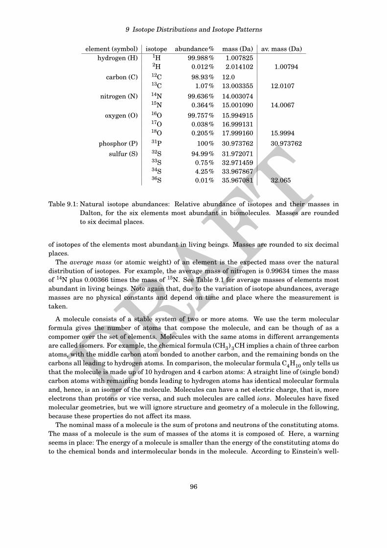
It is important to notice that unlike other numbers in this section, abundances of naturalisotopes are no physical constants: These abundances vary depending on time and place(continent, planet, solar system) where the sample is taken. In fact, physicists may determinethe offspring of a sample based on its isotope abundances. For example, deuterium (2H)varies in relative abundance from about 0.012% to 0.016% in non-marine organisms [54]. Forcomputational mass spectrometry this is usually irrelevant; we just keep in mind that isotopeabundances are not an “exact science” as masses. Regarding the six elements most abundant inliving beings, see Table 9.1 for a detailed list of all natural isotopes and their relative abundancein nature. Isotopes not listed here have relatively small half-lifes and, hence, are not found innature at significant levels. At the end of this chapter, Table 9.5 on page 109 provides the sameinformation for less frequent elements.

Recall that 1 Dalton is 1/12 of the mass of one atom of the 12C isotope, so

1Dalton≈ 1.660538 ·10−24 g and 1g= NA Dalton

where NA ≈ 6.022141 ·1023 denotes the Avogadro constant.Also recall that due to the mass defect, an atoms mass is smaller than sum of masses of the

contained protons, neutrons, and electrons. For example, the mass of a protons is 1.00728 Da,the mass of a neutron 1.00866 Da, and the mass of an electron is about 0.00054 Da. So, 6 protons,6 neutrons, and 6 electrons have a total mass of 12.09596 Da whereas the corresponding 12Catom has a mass of exactly 12 Da, a deviation of about 0.8%. See Table 9.1 above for the masses

1In this book, the term “monoisotopic” consistently refers to the lightest natural isotope, not the most abundantisotope. Otherwise, the monoisotopic masses of the atoms constituting a molecule, will in general not add up tothe monoisotopic mass of the molecule.

95

DRAFT


element (symbol) isotope abundance% mass (Da) av. mass (Da)hydrogen (H) 1H 99.988% 1.007825

2H 0.012% 2.014102 1.00794carbon (C) 12C 98.93% 12.0

13C 1.07% 13.003355 12.0107nitrogen (N) 14N 99.636% 14.003074

15N 0.364% 15.001090 14.0067oxygen (O) 16O 99.757% 15.994915

17O 0.038% 16.99913118O 0.205% 17.999160 15.9994

phosphor (P) 31P 100% 30.973762 30.973762sulfur (S) 32S 94.99% 31.972071

33S 0.75% 32.97145934S 4.25% 33.96786736S 0.01% 35.967081 32.065

Table 9.1: Natural isotope abundances: Relative abundance of isotopes and their masses inDalton, for the six elements most abundant in biomolecules. Masses are roundedto six decimal places.

of isotopes of the elements most abundant in living beings. Masses are rounded to six decimalplaces.

The average mass (or atomic weight) of an element is the expected mass over the naturaldistribution of isotopes. For example, the average mass of nitrogen is 0.99634 times the massof 14N plus 0.00366 times the mass of 15N. See Table 9.1 for average masses of elements mostabundant in living beings. Note again that, due to the variation of isotope abundances, averagemasses are no physical constants and depend on time and place where the measurement istaken.

A molecule consists of a stable system of two or more atoms. We use the term molecularformula gives the number of atoms that compose the molecule, and can be though of as acompomer over the set of elements. Molecules with the same atoms in different arrangementsare called isomers. For example, the chemical formula (CH3) 3CH implies a chain of three carbonatoms, with the middle carbon atom bonded to another carbon, and the remaining bonds on thecarbons all leading to hydrogen atoms. In comparison, the molecular formula C4H10 only tells usthat the molecule is made up of 10 hydrogen and 4 carbon atoms: A straight line of (single bond)carbon atoms with remaining bonds leading to hydrogen atoms has identical molecular formulaand, hence, is an isomer of the molecule. Molecules can have a net electric charge, that is, moreelectrons than protons or vice versa, and such molecules are called ions. Molecules have fixedmolecular geometries, but we will ignore structure and geometry of a molecule in the following,because these properties do not affect its mass.

The nominal mass of a molecule is the sum of protons and neutrons of the constituting atoms.The mass of a molecule is the sum of masses of the atoms it is composed of. Here, a warningseems in place: The energy of a molecule is smaller than the energy of the constituting atoms doto the chemical bonds and intermolecular bonds in the molecule. According to Einstein’s well-

96

DRAFT


12C 13C 1H 2H 16O 17O 18O nom. mass mass (Da) abundance %12 0 22 0 11 0 0 342 342.116215 84.920411 1 22 0 11 0 0 343 343.119570 11.438412 0 22 0 10 1 0 343 343.120431 0.355812 0 21 1 11 0 0 343 343.122492 0.280312 0 22 0 10 0 1 344 344.120460 1.872710 2 22 0 11 0 0 344 344.122925 0.706211 1 22 0 10 1 0 344 344.123786 0.047911 1 21 1 11 0 0 344 344.124647 0.000712 0 22 0 9 2 0 344 344.125847 0.037812 0 21 1 10 1 0 344 344.126708 0.001212 0 20 2 11 0 0 344 344.128769 0.0004

Table 9.2: Isotope species of sucrose molecules C12H22O11, sorted by mass. Isotope species withnominal mass 345 and above omitted.

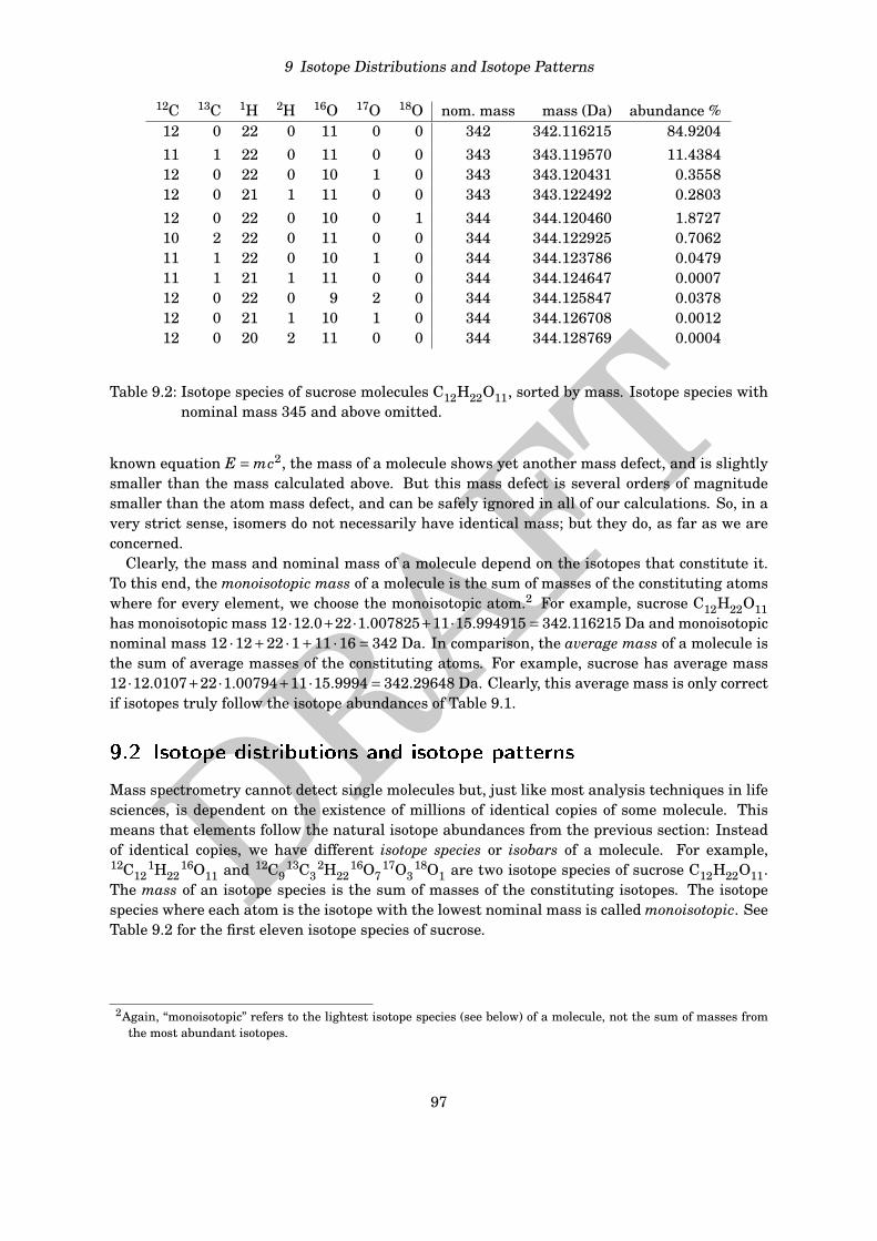
known equation E = mc2, the mass of a molecule shows yet another mass defect, and is slightlysmaller than the mass calculated above. But this mass defect is several orders of magnitudesmaller than the atom mass defect, and can be safely ignored in all of our calculations. So, in avery strict sense, isomers do not necessarily have identical mass; but they do, as far as we areconcerned.

Clearly, the mass and nominal mass of a molecule depend on the isotopes that constitute it.To this end, the monoisotopic mass of a molecule is the sum of masses of the constituting atomswhere for every element, we choose the monoisotopic atom.2 For example, sucrose C12H22O11has monoisotopic mass 12·12.0+22·1.007825+11·15.994915= 342.116215 Da and monoisotopicnominal mass 12 ·12+22 ·1+11 ·16= 342 Da. In comparison, the average mass of a molecule isthe sum of average masses of the constituting atoms. For example, sucrose has average mass12 ·12.0107+22 ·1.00794+11 ·15.9994= 342.29648 Da. Clearly, this average mass is only correctif isotopes truly follow the isotope abundances of Table 9.1.

9.2 Isotope distributions and isotope patterns

Mass spectrometry cannot detect single molecules but, just like most analysis techniques in lifesciences, is dependent on the existence of millions of identical copies of some molecule. Thismeans that elements follow the natural isotope abundances from the previous section: Insteadof identical copies, we have different isotope species or isobars of a molecule. For example,12C12

1H2216O11 and 12C9

13C32H22

16O717O3

18O1 are two isotope species of sucrose C12H22O11.The mass of an isotope species is the sum of masses of the constituting isotopes. The isotopespecies where each atom is the isotope with the lowest nominal mass is called monoisotopic. SeeTable 9.2 for the first eleven isotope species of sucrose.

2Again, “monoisotopic” refers to the lightest isotope species (see below) of a molecule, not the sum of masses fromthe most abundant isotopes.

97

DRAFT


The number of distinct isotope species of a molecule is

number of isotope species= (iC +1)(iH +1)(iN +1)

(iO +2

2

)(iS +3

3

)(9.1)

where iE denotes the multiplicity of element E in the molecule, E ∈ C,H,N,O,P,S. This followsbecause for an element E with r natural isotopes, a molecule E l consisting of l atoms of theelement has

(l+r−1r−1

)different isotope species. Note that

(n0)= 1 for all n ∈N. For example, sucrose

has 13 ·23 · (132)= 23322 isotope species.

Mass spectrometry is usually not capable of resolving isotope species with identical nominalmass. Instead, these isotope species appear as one single peak in the MS output. There aretwo exceptions to this rule: Using high-resolution mass spectrometry and analyzing a moleculethat contains sulfur, one can often identify two instead of one peak for monoisotopic nominalmass plus 2. The same problem exists for other elements whose isotope mass differences differsignificantly from that of carbon. See Sec. 9.4 for more details. For the moment, we simplyignore this problem.

Second, if the nominal mass of an isotope species is significantly larger than the monoisotopicnominal mass, then isotope species with distinct nominal masses may have almost identicalreal masses. Consider the molecular formula C345H344 with nominal monoisotopic mass 4484:the isotope species 13C345

1H344 has nominal mass 4828 and mass 4832.849275 Da whereas theisotope species 12C345

2H344 has nominal mass 4827 and mass 4832.851088 Da. As we will see,we can usually limit calculations to isotope species with nominal mass no more than, say, tenabove the monoisotopic nominal mass, for all molecules that are of interest to us. Hence, wemay safely ignore this subtlety.

We merge isotope species with identical nominal mass; we refer to the resulting distributionas the molecule’s isotope distribution (or isotopic distribution). How can we formally model thisisotope distribution? For each element E ∈Σ we define a discrete random variable, denoted YE,representing the nominal mass distribution of the element. For example, YC with state space12,13 and

P(YC = 12

)= 0.98890, P(YC = 13

)= 0.01110

is the random variables of carbon, whereas YO with state space 16,17,18 and

P(YO = 16

)= 0.99757, P(YO = 17

)= 0.00038, P(YO = 18

)= 0.00205

is the random variable of oxygen.Now, the random variable Y of a molecule is the sum of random variables of the atoms

constituting the molecule, where we choose these random variables according to the elementof each atom. Unfortunately, we have to deal with a subtlety in the stochastic notation: Wecannot write YH2O =YH+YH+YO for the isotope distribution of H2O, as this would not result intwo independent random variables for hydrogen but instead, one random variable whose valueis doubled. To this end, we have two go a slightly longer road. We write Y ∼ Y ′ if two randomvariables are independent identically distributed. So, P(Y = y) = P(Y ′ = y) holds for all y in thestate space, but Y and Y ′ are independent. Given a molecule consisting of l atoms, we assign toeach atom i a random variable Yi, for i = 1, . . . , l, such that Yi ∼ YE i where E i is the element ofthe ith atom. Now we can represent the molecule’s isotope distribution by the random variableY :=Y1 + . . .+Yl .

98

DRAFT


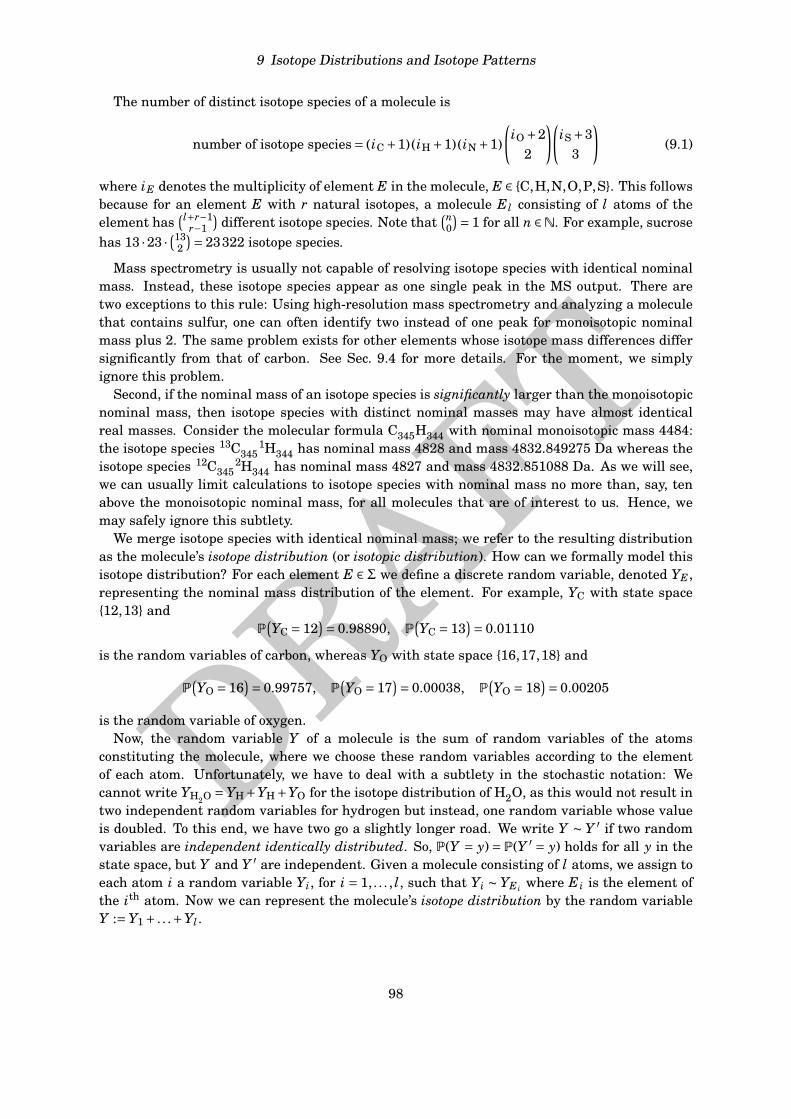
nominal mass 342 343(+1) 344(+2) 345(+3) 346(+4) 347. . .398abundance % 84.9204 12.0745 2.6668 0.2976 0.0371 < 0.0001

Table 9.3: Isotope distribution of sucrose C12H22O11 in percent, rounded to four decimal places.

Example 9.1. Consider sucrose with molecular formula C12H22O11. The isotope distribution ofsucrose is the random variable Y =Y1 +·· ·+Y45 where

Yi ∼YC for i = 1, . . . ,12,

Y12+i ∼YH for i = 1, . . . ,22, and

Y34+i ∼YO for i = 1, . . . ,11.

In an ideal mass spectrum, normalized peak intensities correspond to the isotope distributionof the molecule. For ease of exposition, the peak at monoisotopic mass is also called monoisotopic,the following peaks are referred to as +1, +2, . . . peaks. The number of non-zero entries in theisotope distribution of a molecule is

number non-zero entries= iC + iH + iN +2iO +3iS +1 (9.2)

where again, iE denotes the multiplicity of element E in the molecule, E ∈ C,H,N,O,P,S.Clearly, this is much less than the number of isotope species, compare to (9.1): For example,sucrose C12H22O11 has 12+22+2 ·11+1= 57 non-zero entries, ranging from nominal mass 342to 398. See Table 9.3 for the isotope distribution of sucrose. Put differently, if Y is the randomvariable of sucrose, then P(Y = 342) = 0.8492. Peak intensity quickly deteriorate for increasingnominal mass, and P(Y ≥ 347)< 0.00004.

So, the imperfection of mass spectrometry results in +1,+2, . . . isotope peaks that, in fact, aresuperpositions of peaks with almost identical mass. We have introduced above a model for theintensity of the superimposed peak; but what about its mass? It is reasonable to assume thatthe mass of a peak in the isotope pattern, is the mean mass of all isotope species that add toits intensity. We now formalize this idea: For each element E ∈ Σ we define another randomvariable XE, representing the mass of the natural isotopes. Random variables XE and YE arecorrelated: In fact, XE can be viewed as a function λ of YE and E, XE = λE(YE). For example,XC with state space 12,13.003355 and

P(XC = 12

)= 0.98890, P(XC = 13.003355

)= 0.01110

is the random variables of carbon, and we have XC = 12 if and only if YC = 12. Given a moleculeconsisting of l atoms, we assign to the ith atom, i = 1, . . . , l, a random variables X i such thatX i ∼ XE i , where E i is the element of the ith atom. Now we can represent the molecule’s massdistribution by the random variable X := X1+ . . .+X l . Clearly, X and Y are correlated, where Yis the isotope distribution of the molecule.

For mass distribution X = X1 + . . .+ X l and isotopic distribution Y =Y1 +·· ·+Yl of a moleculewith elements E1, . . . ,E l and monoisotopic nominal mass N, the mean peak mass mn of the +npeak can be calculated as:

mn = E(X∣∣ Y = N +n

)= ∑∑

i Ni=N+n

P(Y1 = N1, . . . ,Yl = Nl)P(Y = N +n)

(λ(N1,E1)+·· ·+λ(Nl ,E l)

) (9.3)

99

DRAFT


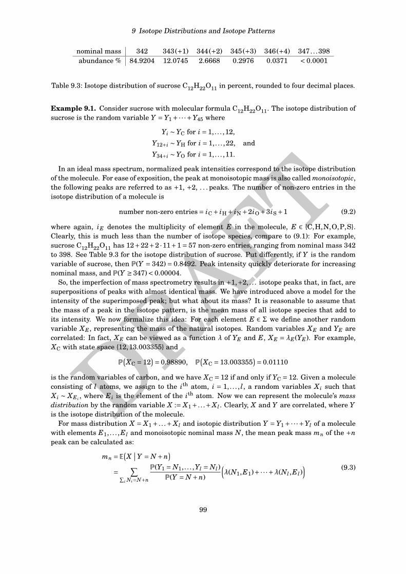
nominal mass 342 343(+1) 344(+2) 345(+3) 346(+4)abundance % 84.9204 12.0745 2.6668 0.2976 0.0371

mean peak mass 342.116215 343.119663 344.121254 345.124197 346.126084

Table 9.4: Isotope pattern (isotopic distribution and mean peak masses) of sucrose C12H22O11.Peaks with nominal mass 347, . . . ,398 have abundances of less than 0.01%.

where the sum is taken over all vectors ~N = (N1, . . . , Nl) ∈Nl satisfying∑

i Ni = N+n. We refer tothe isotope distribution together with the mean peak masses as the molecule’s isotope pattern.See Table 9.4 for the isotope pattern of sucrose.

9.3 Simulating isotope patterns

In the following, we will “separate” isotope patterns from the monoisotopic nominal mass ofthe molecule: If two molecular formulas differ by a single phosphor atom, then the resultingisotope patterns are identical, only shifted by the mass of a single phosphor. In other words:It is of no interest for the isotope pattern what the actual nominal mass N of the molecule is.To this end, we write nominal masses of isotopes as N +n, corresponding to the +n peak of theisotope pattern. The monoisotopic peak will also be referred to as “the first non-zero value of thedistribution” because obviously, no isotope can have smaller mass.

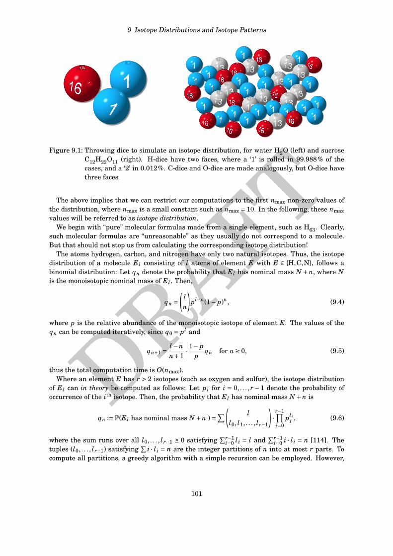
We start with the computation of the isotope distribution, as this will be needed to computemean peak masses. Let us compute the isotope distribution of sucrose C12H22O11 by hand,compare to Table 9.3. To do so, we put 100 000 marbles in a bag: 99 988 will be marked “1” and12 marbles will be marked “2”. We label the bag with an ‘H’. We prepare a second bag labeled ‘C’that contains 9 893 marbles marked “12” and 107 marbles marked “13”. In a third bag labeled ‘O’we put 99 757 marbles marked “16”, 38 marbles marked “17”, and 205 marbles marked “18”. Atrandom, pull a marble from the sack labeled ‘C’, write down the number, put it back. Repeat 11more times. Do the same for sack ‘H’ with 22 repetitions, and for the sack ‘O’ with 11 repetitions.Sum up all numbers, record the sum on a second piece of paper. Repeat 10 000 times, count howoften you have computed each sum — voilá, you have just simulated an isotope distribution.Another way to do this is throwing dice, see Fig. 9.1. Obviously, these two methods are notvery helpful to simulate isotope distributions, neither by hand nor in the computer: Doing sois not only time consuming but, even worse, the simulated isotope distribution can still differsignificantly from the distribution you would get for an infinite number of repetitions. Can wedo better?

Computing the complete isotope distribution is somewhat tedious, as there are many inten-sities that we compute in vain, see again Table 9.3 where peaks at nominal masses 347 to 398will not be detectable in any mass spectrometer. In fact, isotope distributions decrease rapidlyfor all molecules over the alphabet of elements CHNOPS. To further substantiate this claimempirically, we extracted all molecular formulas from the KEGG COMPOUND database [124](release 42.0) that have elements CHNOPS and mass below 3000 Da. Amongst the resulting11479 molecular formulas, not a single entry has intensity of the +10 peak larger than 0.007%.Clearly, the corresponding peak must be lost in the noise of the experimental mass spectrum.We consider the worst case of a “sulfur-only” molecule in Exercise 9.1.

100

DRAFT


Figure 9.1: Throwing dice to simulate an isotope distribution, for water H2O (left) and sucroseC12H22O11 (right). H-dice have two faces, where a ‘1’ is rolled in 99.988% of thecases, and a ‘2’ in 0.012%. C-dice and O-dice are made analogously, but O-dice havethree faces.

The above implies that we can restrict our computations to the first nmax non-zero values ofthe distribution, where nmax is a small constant such as nmax = 10. In the following, these nmaxvalues will be referred to as isotope distribution.

We begin with “pure” molecular formulas made from a single element, such as H63. Clearly,such molecular formulas are “unreasonable” as they usually do not correspond to a molecule.But that should not stop us from calculating the corresponding isotope distribution!

The atoms hydrogen, carbon, and nitrogen have only two natural isotopes. Thus, the isotopedistribution of a molecule E l consisting of l atoms of element E with E ∈ H,C,N, follows abinomial distribution: Let qn denote the probability that E l has nominal mass N +n, where Nis the monoisotopic nominal mass of E l . Then,

qn =(

ln

)pl−n(1− p)n, (9.4)

where p is the relative abundance of the monoisotopic isotope of element E. The values of theqn can be computed iteratively, since q0 = pl and

qn+1 = l−nn+1

· 1− pp

qn for n ≥ 0, (9.5)

thus the total computation time is O(nmax).Where an element E has r > 2 isotopes (such as oxygen and sulfur), the isotope distribution

of E l can in theory be computed as follows: Let pi for i = 0, . . . , r−1 denote the probability ofoccurrence of the ith isotope. Then, the probability that E l has nominal mass N +n is

qn :=P(E l has nominal mass N +n )=∑(l

l0, l1, . . . , lr−1

)·

r−1∏i=0

pl ii , (9.6)

where the sum runs over all l0, . . . , lr−1 ≥ 0 satisfying∑r−1

i=0 l i = l and∑r−1

i=0 i · l i = n [114]. Thetuples (l0, . . . , lr−1) satisfying

∑i · l i = n are the integer partitions of n into at most r parts. To

compute all partitions, a greedy algorithm with a simple recursion can be employed. However,

101

DRAFT


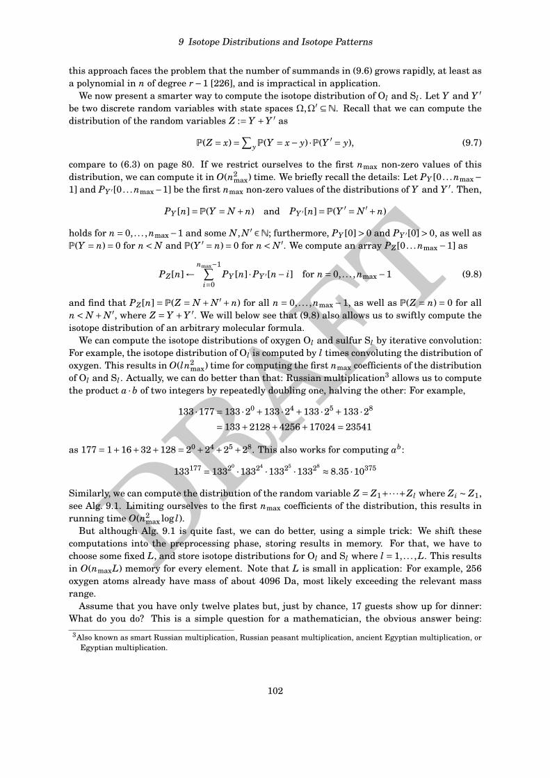
this approach faces the problem that the number of summands in (9.6) grows rapidly, at least asa polynomial in n of degree r−1 [226], and is impractical in application.

We now present a smarter way to compute the isotope distribution of Ol and Sl . Let Y and Y ′

be two discrete random variables with state spaces Ω,Ω′ ⊆ N. Recall that we can compute thedistribution of the random variables Z :=Y +Y ′ as

P(Z = x)=∑yP(Y = x− y) ·P(Y ′ = y), (9.7)

compare to (6.3) on page 80. If we restrict ourselves to the first nmax non-zero values of thisdistribution, we can compute it in O(n2

max) time. We briefly recall the details: Let PY [0. . .nmax−1] and PY ′[0. . .nmax−1] be the first nmax non-zero values of the distributions of Y and Y ′. Then,

PY [n]=P(Y = N +n) and PY ′[n]=P(Y ′ = N ′+n)

holds for n = 0, . . . ,nmax−1 and some N, N ′ ∈N; furthermore, PY [0]> 0 and PY ′[0]> 0, as well asP(Y = n)= 0 for n < N and P(Y ′ = n)= 0 for n < N ′. We compute an array PZ[0. . .nmax −1] as

PZ[n]←nmax−1∑

i=0PY [n] ·PY ′[n− i] for n = 0, . . . ,nmax −1 (9.8)

and find that PZ[n] = P(Z = N +N ′+n) for all n = 0, . . . ,nmax −1, as well as P(Z = n) = 0 for alln < N +N ′, where Z = Y +Y ′. We will below see that (9.8) also allows us to swiftly compute theisotope distribution of an arbitrary molecular formula.

We can compute the isotope distributions of oxygen Ol and sulfur Sl by iterative convolution:For example, the isotope distribution of Ol is computed by l times convoluting the distribution ofoxygen. This results in O(ln2

max) time for computing the first nmax coefficients of the distributionof Ol and Sl . Actually, we can do better than that: Russian multiplication3 allows us to computethe product a ·b of two integers by repeatedly doubling one, halving the other: For example,

133 ·177= 133 ·20 +133 ·24 +133 ·25 +133 ·28

= 133+2128+4256+17024= 23541

as 177= 1+16+32+128= 20 +24 +25 +28. This also works for computing ab:

133177 = 13320 ·13324 ·13325 ·13328 ≈ 8.35 ·10375

Similarly, we can compute the distribution of the random variable Z = Z1+·· ·+Zl where Zi ∼ Z1,see Alg. 9.1. Limiting ourselves to the first nmax coefficients of the distribution, this results inrunning time O(n2

max log l).But although Alg. 9.1 is quite fast, we can do better, using a simple trick: We shift these

computations into the preprocessing phase, storing results in memory. For that, we have tochoose some fixed L, and store isotope distributions for Ol and Sl where l = 1, . . . ,L. This resultsin O(nmaxL) memory for every element. Note that L is small in application: For example, 256oxygen atoms already have mass of about 4096 Da, most likely exceeding the relevant massrange.

Assume that you have only twelve plates but, just by chance, 17 guests show up for dinner:What do you do? This is a simple question for a mathematician, the obvious answer being:

3Also known as smart Russian multiplication, Russian peasant multiplication, ancient Egyptian multiplication, orEgyptian multiplication.

102

DRAFT


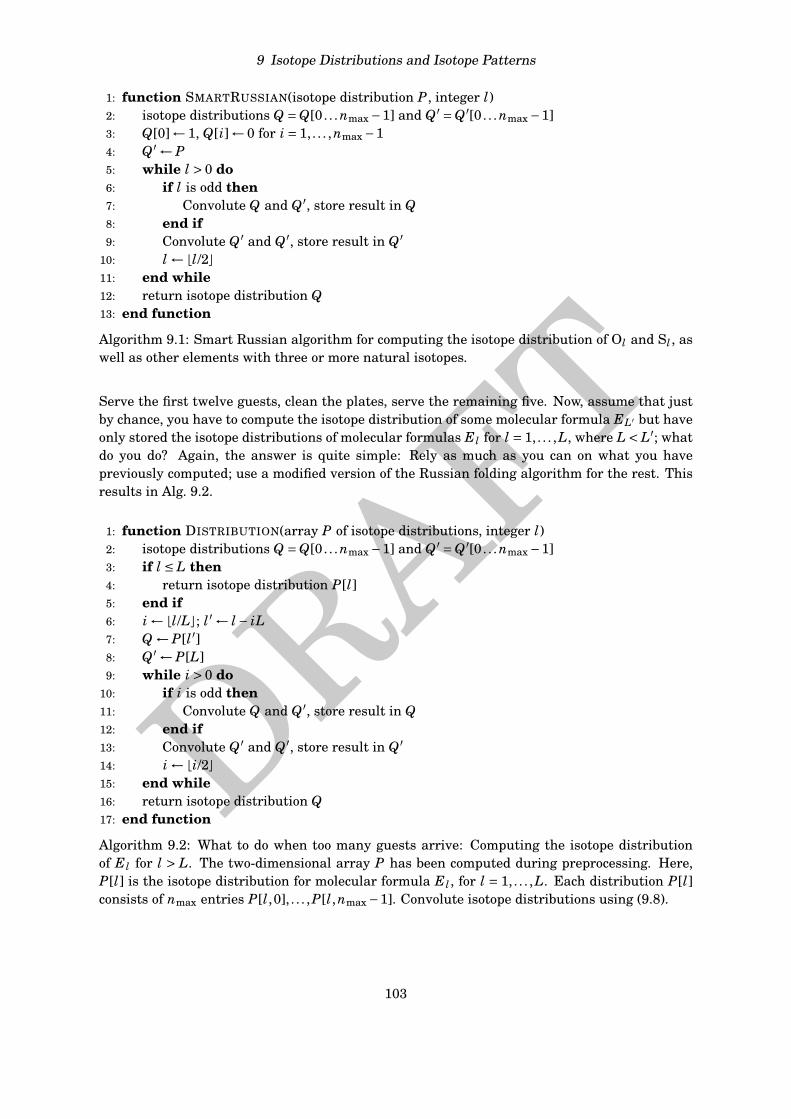
1: function SMARTRUSSIAN(isotope distribution P, integer l)2: isotope distributions Q =Q[0. . .nmax −1] and Q′ =Q′[0. . .nmax −1]3: Q[0]← 1, Q[i]← 0 for i = 1, . . . ,nmax −14: Q′ ← P5: while l > 0 do6: if l is odd then7: Convolute Q and Q′, store result in Q8: end if9: Convolute Q′ and Q′, store result in Q′

10: l ←bl/2c11: end while12: return isotope distribution Q13: end function

Algorithm 9.1: Smart Russian algorithm for computing the isotope distribution of Ol and Sl , aswell as other elements with three or more natural isotopes.

Serve the first twelve guests, clean the plates, serve the remaining five. Now, assume that justby chance, you have to compute the isotope distribution of some molecular formula EL′ but haveonly stored the isotope distributions of molecular formulas E l for l = 1, . . . ,L, where L < L′; whatdo you do? Again, the answer is quite simple: Rely as much as you can on what you havepreviously computed; use a modified version of the Russian folding algorithm for the rest. Thisresults in Alg. 9.2.

1: function DISTRIBUTION(array P of isotope distributions, integer l)2: isotope distributions Q =Q[0. . .nmax −1] and Q′ =Q′[0. . .nmax −1]3: if l ≤ L then4: return isotope distribution P[l]5: end if6: i ←bl/Lc; l′ ← l− iL7: Q ← P[l′]8: Q′ ← P[L]9: while i > 0 do

10: if i is odd then11: Convolute Q and Q′, store result in Q12: end if13: Convolute Q′ and Q′, store result in Q′

14: i ←bi/2c15: end while16: return isotope distribution Q17: end function

Algorithm 9.2: What to do when too many guests arrive: Computing the isotope distributionof E l for l > L. The two-dimensional array P has been computed during preprocessing. Here,P[l] is the isotope distribution for molecular formula E l , for l = 1, . . . ,L. Each distribution P[l]consists of nmax entries P[l,0], . . . ,P[l,nmax −1]. Convolute isotope distributions using (9.8).

103

DRAFT


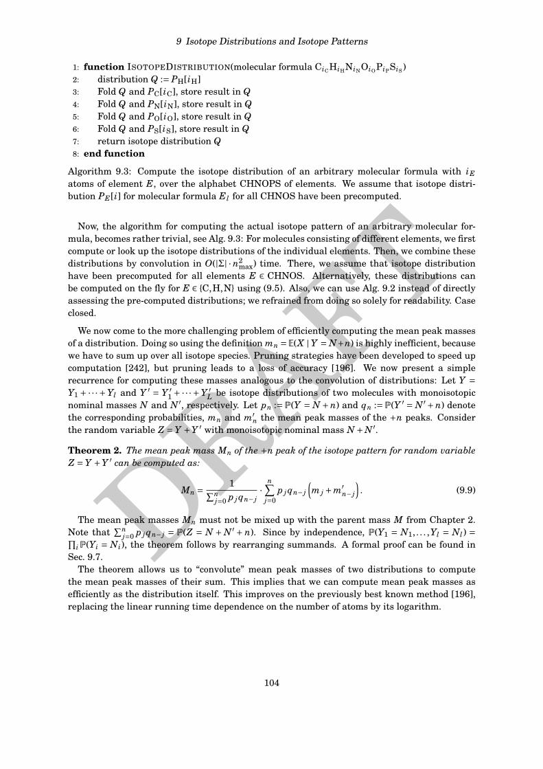
1: function ISOTOPEDISTRIBUTION(molecular formula CiCHiHNiNOiOPiPSiS)2: distribution Q := PH[iH]3: Fold Q and PC[iC], store result in Q4: Fold Q and PN[iN], store result in Q5: Fold Q and PO[iO], store result in Q6: Fold Q and PS[iS], store result in Q7: return isotope distribution Q8: end function

Algorithm 9.3: Compute the isotope distribution of an arbitrary molecular formula with iEatoms of element E, over the alphabet CHNOPS of elements. We assume that isotope distri-bution PE[i] for molecular formula E l for all CHNOS have been precomputed.

Now, the algorithm for computing the actual isotope pattern of an arbitrary molecular for-mula, becomes rather trivial, see Alg. 9.3: For molecules consisting of different elements, we firstcompute or look up the isotope distributions of the individual elements. Then, we combine thesedistributions by convolution in O(|Σ| · n2

max) time. There, we assume that isotope distributionhave been precomputed for all elements E ∈ CHNOS. Alternatively, these distributions canbe computed on the fly for E ∈ C,H,N using (9.5). Also, we can use Alg. 9.2 instead of directlyassessing the pre-computed distributions; we refrained from doing so solely for readability. Caseclosed.

We now come to the more challenging problem of efficiently computing the mean peak massesof a distribution. Doing so using the definition mn = E(X |Y = N+n) is highly inefficient, becausewe have to sum up over all isotope species. Pruning strategies have been developed to speed upcomputation [242], but pruning leads to a loss of accuracy [196]. We now present a simplerecurrence for computing these masses analogous to the convolution of distributions: Let Y =Y1 + ·· · +Yl and Y ′ = Y ′

1 + ·· · +Y ′L be isotope distributions of two molecules with monoisotopic

nominal masses N and N ′, respectively. Let pn := P(Y = N +n) and qn := P(Y ′ = N ′+n) denotethe corresponding probabilities, mn and m′

n the mean peak masses of the +n peaks. Considerthe random variable Z =Y +Y ′ with monoisotopic nominal mass N +N ′.

Theorem 2. The mean peak mass Mn of the +n peak of the isotope pattern for random variableZ =Y +Y ′ can be computed as:

Mn = 1∑nj=0 p j qn− j

·n∑

j=0p j qn− j

(m j +m′

n− j

). (9.9)

The mean peak masses Mn must not be mixed up with the parent mass M from Chapter 2.Note that

∑nj=0 p j qn− j = P(Z = N + N ′ + n). Since by independence, P(Y1 = N1, . . . ,Yl = Nl) =∏

iP(Yi = Ni), the theorem follows by rearranging summands. A formal proof can be found inSec. 9.7.

The theorem allows us to “convolute” mean peak masses of two distributions to computethe mean peak masses of their sum. This implies that we can compute mean peak masses asefficiently as the distribution itself. This improves on the previously best known method [196],replacing the linear running time dependence on the number of atoms by its logarithm.

104

DRAFT


9.4 Sulfur and other mavericks

What is so special about sulfur, that we have to treat it different than the other elements? First,look at the mass difference: The mass difference µ(13C)−µ(12C)= 1.003355 is larger than one, sothe isotope peaks of a carbon molecule are farther to the “right” than nominal masses suggest. Incontrast, µ(34S)−µ(32S)= 1.995796, so isotope peaks of a sulfur molecule are farther to the “left”than nominal masses suggest. But nitrogen and even hydrogen also show strong deviations inthe mass difference of isotopes, and we do not treat them separately. So, what is special aboutsulfur?

The answer is somewhat more subtle: Our assumption that an isotope peak is a superpositionof all isotope species with identical nominal mass, only holds if mass differences betweensubsequent isotope species is small, or if intensities of outlier isotope species are very small.

See Table 9.2 for the isotope species of sucrose: There are seven isotope species with nominalmass 344, ranging in mass from 344.120460 to 344.128769, an interval of 0.008309 Da width.But the mass difference between any two subsequent isotope species is much smaller, namely0.002465 at maximum. Now, this mass difference is below 1 ppm, and even though resolvingpeaks is a matter of resolution (see Chapter 7) and not of mass accuracy, it should be easy tobelieve that such peaks can easily “smear” into a single peak in a mass spectrum.

Now, let us the gedankenexperiment that the molecular formula contains an additional sulfurwith nominal mass 32 — what are the resulting isotope species with nominal mass 344+32 =376? The isotope species that use the 32S sulfur isotope, are the same as those displayed inTable 9.2, only shifted by 31.972071, and range from 376.092531 to 376.100840. The 33S isotopeof sulfur will result in several additional isotope species of low intensity, that we may ignore.But the 34S isotope of sulfur results in a single isotope species with mass 376.084082, at distance0.008449 Da to the closest isotope species.

[TODO: REPLACE GEDANKENEXPERIMENT BY SOMETHING REAL: SIMULATE ISOTOPESPECIES FOR A MOLECULE WITH AND WITHOUT SULFUR]

[TODO: DESCRIBE HOW TO FOLD TWO LISTS OF ISOTOPE SPECIES]

9.5 Isotope patterns of peptides

Obvious way: Compute molecular formula of the peptide, simulate the isotope pattern using themethods from Sec. 9.3. It turns out that this is also the fastest method to do so.

Precompute isotope patterns for each amino acid – not a good idea, rather compute themolecular formula first, than the isotope pattern. Needs about 3n2

max multiplications forcomputing the isotope distribution. Directly folding the isotope patterns of each amino acid,even if we store all of these distributions in memory, requires roughly 9.5n2

max multiplicationsfor the isotope distribution.

9.6 Isotope labeling

9.7 Formal proof of the folding theorem

For the sake of completeness, we now provide a formal proof of Theorem 2. The proof is verysimple in its essence, yet formally sophisticated. Readers not interested in the formal detailscan safely skip this section.

105

DRAFT


Let ~N = (N1, . . . , Nl) ∈Nl and ~N ′ = (N ′1, . . . , N ′

L) ∈NL be vectors of nominal masses. We denote∑ ~N := ∑li=1 Ni and

∑ ~N ′ := ∑Li=1 N ′

i. Let ~Y := (Y1, . . . ,Yl) and ~Y ′ := (Y ′1, . . . ,Y ′

L) be vectors of theinput random variables, and note that

P(~Y = ~N, ~Y ′ = ~N ′)=P(~Y = ~N)P(~Y ′ = ~N ′)

due to the independence of the underlying random variables. Finally, we set λ(~N)=∑li=1λE i (Ni)

and analogously define λ(~N ′).We can rewrite (9.3) for the mass of the +n peak as

P(Z = N +N ′+n) ·Mn = ∑∑ ~N+∑ ~N ′=N+N ′+n

P(~Y = ~N, ~Y ′ = ~N ′) · (λ(~N)+λ(~N ′)).

We observe that we can split this formula into two independent sums of the form∑∑ ~N+∑ ~N ′=N+N ′+n

P(~Y = ~N, ~Y ′ = ~N ′) ·λ(~N) (9.10)

and a second summand where λ(~N) is replaced by λ(~N ′); we concentrate on (9.10) in thefollowing. Now, ∑

∑ ~N+∑ ~N ′=N+N ′+n

P(~Y = ~N, ~Y ′ = ~N ′) ·λ(~N)

=n∑

j=0

∑∑ ~N=N+ j

∑∑ ~N ′=N ′+n− j

P(~Y = ~N)P(~Y ′ = ~N ′) ·λ(~N)

=n∑

j=0

∑∑ ~N=N+ j

P(~Y = ~N) ·λ(~N)∑

∑ ~N ′=N ′+n− j

P(~Y ′ = ~N ′)

=n∑

j=0

∑∑ ~N=N+ j

P(~Y = ~N) ·λ(~N) ·P(Y ′1 +·· ·+Y ′

L = N ′+n− j)

=n∑

j=0P(Y ′ = N ′+n− j)

∑∑ ~N=N+ j

P(~Y = ~N) ·λ(~N)

=n∑

j=0qn− j p jm j

where the last equality follows from the definition of m j,

m j = 1p j

∑∑ ~N=N+ j

P(~Y = ~N) ·λ(~N).

Analogously, we can show that

∑∑ ~N+∑ ~N ′=N+N ′+n

P(~Y = ~N, ~Y ′ = ~N ′) ·λ(~N ′)=n∑

j=0qn− j p jm′

j.

This concludes the proof of the theorem.

106

DRAFT


9.8 Historical notes and further reading

The formalism and methods presented in this chapter follow the paper of Böcker, Letzel, Lipták,and Pervukhin [29], but note that some variable names have been changed: Here, we use n, Nfor the nominal masses of the molecule, whereas k is the size of the alphabet.

[TODO: WHAT ABOUT [114]?]Back in 1991, Kubinyi [138] suggested to compute isotope distributions by convoluting isotope

distributions of “hyperatoms” using, in principle, the smart Russian algorithm from Alg. 9.1.In the literature on simulating isotope distributions and patterns, one can find many con-

tributions by Alan L. Rockwood: Rockwood et al. [195] suggested to use mean peak massesas the masses of isotope peaks. Later, Rockwood et al. [196] presented some validation of thishypothesis, as well as an algorithm for computing mean peak masses, which is more complicatedand less efficient than the algorithm from Sec. 9.3. In 2006, Rockwood and Haimi [194] andBöcker, Letzel, Lipták, and Pervukhin [27] independently came up with the algorithm presentedin Sec. 9.3.

A huge number of software packages have been developed for simulating isotope patternsover time [1, 77, 216, 219]. At most, these programs offer means to visually compare a measuredspectrum with a simulated isotope pattern. Also, some authors appear to be unaware of methodsfor swiftly simulating isotope distributions and patterns [27, 138, 194]. [TODO: CHECKEN,SONST UNHOEFLICH]

We have seen in Chapter 2 that we often record the fragmentation pattern of a molecule,to obtain additional information about its structure. Usually, only the monoisotopic peak isselected for fragmentation, to simplify the interpretation of the fragmentation spectra. But whatif we select, say, the monoisotopic and the +1 peak for simultaneous fragmentation? Obviously,the isotope distribution of fragments is not the isotope distribution of a “regular” molecule.Somewhat surprisingly, it is not too complicated to simulate these isotope distributions, seeRockwood, Kushnir, and Nelson [195] and Exercise 9.8. On the downside, simulating suchtruncated isotope distributions requires considerably more time than the algorithms fromSec. 9.3. In contrast, if one opens the parent mass window wide enough so that all “important”isotope peaks are selected for fragmentation, then isotope distributions of fragments will followthe isotope distribution as defined in Sec. 9.2. But this will increase the chance that besidesthe isotope peak of the molecule of interest, other molecules may “sneak” into the fragmentationprocess.

Masses of isotopes are taken the paper of Audi, Wapstra, and Thibault [5] and rounded tosix decimal places, see there for a complete table, and Wieser [233] for corrections. Isotopeabundances and atomic weight (average masses) taken from the paper of de Laeter et al. [54].See de Laeter et al. [54] for the history of atomic-weight determination.

Warning: The masses given in this chapter are not meant for the use in computer programs,but rather for the human reader. This might become an issue as soon as you want to analyzespectra with mass accuracy below, say, 1 ppm. Instead, you should download masses with highermass accuracy from the Internet.4

Computations throughout this chapter use masses from Table 9.1. In contrast, Table 2.1 hasnot been computed using Table 9.1 but instead, higher accuracy masses have been used. Forexample, a cysteine residue has mass 103.009184 according to Table 2.1, whereas C3H5N1O1S1has mass 103.009185 according to Table 9.1.

4http://

107

DRAFT


See Table 9.5 for isotope masses of less abundant elements: These include fluorine (F, 9),silicon (Si, 14), and zinc (Zn, 30). Boron (B, 5) is a trace mineral in humans, and is believed to beinvolved in carbohydrate transport in plants. Chlorine (Cl, 17) is necessary for osmosis and ionicbalance, and important for pharmaceuticals. Copper (Cu, 29) is incorporated in certain proteins.Selenium (Se, 34) is a micronutrient for animals and component of the non-proteinogenic aminoacid selenocysteine. Bromine (Br, 35) and iodine (I, 53) can be found in drugs and hormones; theformer is also important for pharmaceuticals. Tungsten (W, 74), also known as Wolfram, is anessential nutrient for some organisms.

[TODO: CALCIUM UND EISEN SIND BIOLOGISCH AUCH NOCH WICHTIG.]

9.9 Exercises

9.1 Imagine a “sulfur-only” molecule — how large does this molecule have to be, so thatthe +10 has intensity of more the 1%? This can be seen as a worst-case scenario. Foryour computation, assume that sulfur has only two isotopes, namely nominal mass 34with relative abundance 1− p = 0.0425, and nominal mass 32 with relative abundance p.Estimate the required number of sulfur atoms using (9.4). Be reminded that the heavierisotope of sulfur has nominal mass 34, not 33.

9.2 Write a program to simulate the isotope distribution of an arbitrary molecular formulaover the elements CHNOPS. Compute the isotope distribution of sucrose, and verify yourresult using Table 9.3.

9.3 Verify your calculations from Exercise 9.1 using the program from Exercise 9.2.

9.4 We noted above that amongst all entries in the KEGG COMPOUND database (release42.0) with elements CHNOPS and mass below 3000 Da, not a single molecule has intensityof the +10 peak larger than 0.007%. But that version of the database is totally outdatedby now — possibly, there are new molecular formulas in the current release that have +10peaks of higher intensities?

9.5 A peptide s ∈ Σ∗ is said to be pure if it is made from repetitions of a single amino acid,s = xl for some x ∈Σ. Find the pure peptide with intensity of the +10 peak larger than 1%such that µ(s) is minimum.

9.6 Let s ∈ Σ∗ be any peptide with intensity of the +10 peak larger than 1% such that µ(s) isminimum. This peptide is not necessarily pure. Argue why its mass will be close to themass calculated in the previous exercise.

9.7 In Alg. 9.1 (the smart Russian convolution) you can get rid of two convolutions — how?

9.8? Assume that not only the monoisotopic peak is picked for fragmentation, but also +1 and+2 peaks. Now, fragments will show a truncated isotope pattern, which is obviously notthe full isotope pattern. Let fp, f be the molecular formulas of the parent molecule andthe fragment, and choose f ′ such that f + f ′ = fp. (Here, f ′ is the neutral loss, compareto Chapter 13.) Let Y ,Y ′, Z be the random variables for f , f ′, fp, and let N, N ′, Np bethe corresponding nominal masses. Assume we have picked peaks 0, . . . ,nmax −1 from theparent isotope distribution, or a subset thereof. Then, we can limit our calculations to

108

DRAFT


element (symbol) AN isotope abundance% mass (Da) av. mass (Da)boron (B) 5 10B 19.9∗% 10.012937

11B 80.1∗% 11.009305 10.811fluorine (F) 9 18F 100% 18.000938 18.000938silicon (Si) 14 28Si 92.223% 27.976927

29Si 4.685% 28.97649530Si 3.092% 29.973770 28.0855

chlorine (Cl) 17 35C 75.76% 34.96885337C 24.24% 36.965903 35.453

calcium (Ca) 20 40Ca 96.941% 39.96259142Ca 0.647% 41.95861843Ca 0.135% 42.95876744Ca 2.086% 43.95548246Ca 0.004% 45.95369348Ca 0.187% 47.952534 ??

iron (Fe) 26 54Fe 5.845% 53.93961156Fe 91.754% 55.93493757Fe 2.119% 56.93539458Fe 0.282% 57.933276 ??

copper (Cu) 29 63Cu 69.15% 62.92959765Cu 30.85% 64.927789 63.546

zinc (Zn) 30 64Zn 48.268% 63.92914266Zn 27.975% 65.92603367Zn 4.102% 66.92712768Zn 19.024% 67.92484470Zn 0.631% 69.925319 65.409

selenium (Se) 34 74Se 0.89% 73.92247676Se 9.37% 75.91921477Se 7.63% 76.91991478Se 23.77% 77.91730980Se 49.61% 79.91652182Se 8.73% 81.916699 78.96

bromine (Br) 35 79Br 50.69% 78.91833781Br 49.31% 80.916291 ??

iodine (I) 53 127I 100% 126.904473 126.904473tungsten (W) 74 180W 0.12% 179.946704

182W 26.50% 181.948204183W 14.31% 182.950223184W 30.64% 183.950931186W 28.43% 185.954364 183.84

Table 9.5: Natural isotope abundances of elements less frequent in biomolecules. ‘AN’ is atomicnumber. Masses rounded to six decimal places. *Distribution of boron shows a strongvariation, depending on where the sample is taken.

109

DRAFT


the first nmax peaks of the truncated fragment distributions — explain why. We define amatrix C[0. . .nmax −1,0. . .nmax −1] by

C[i, j] :=P(Y = N + i) ·P(Y ′ = N ′+ j).

Then, P(Z = Np + n) = ∑nj=0 C[ j,n− j] holds. Describe an algorithm that computes the

truncated isotope distribution of fragment f using matrix C and the above equation.

9.9?Try to estimate the abundances of CHNOPS from some database for peptide mass spectra— [TODO: HOW?]

110

DRAFT

10 Decomposing Isotope Patterns

ASSUME that we have measured an isotope pattern, and we want to find those molecularformulas that show the highest similarity the measured pattern, over some fixed alphabet

of elements. Note that the formal definition of “isotope pattern” is, to a certain extend, dependingon the application and the used MS technique, see Sec. 9.2 and 9.4. Unfortunately, decomposingan isotope pattern is a somewhat ill-post problem, and we are not aware of any practicalapproaches that directly address this problem. Instead, we circumvent the problem, similarto the two-step strategy proposed in Sec. 8.4: First, we filter the set of molecular formulasto a manageable subset, using only one or few features of isotope patterns, in particular themonoisotopic mass. This leaves us with a set of candidate molecular formulas. The first stepis not meant to differentiate between the candidates; its only purpose is to quickly generatea candidate set of manageable size. In the next step, we evaluate the candidates using theisotope patterns: As we now have a candidate molecular formula, it is an easy task to simulatethe corresponding isotope pattern using methods from Sec. 9.3, and to compare the simulatedisotope pattern against the the measured one, comparable to a database search. The candidatewith the best match against the measured isotope pattern is the output of our method, andhopefully the correct answer.

High mass accuracy, as required throughout this chapter, is nowadays available from amultitude of MS platforms, such as Fourier Transform Ion Cyclotron Resonance (FR-ICR) MS,Orbitrap MS, or orthogonal Quadrupole Time-of-Flight (QTOF) MS. As a rough estimate, QTOFMS reaches a mass accuracy of 10 ppm or better; Orbitrap reaches 1 ppm or better; and FT-ICRmeasurements can have mass accuracy well below 0.1 ppm. These numbers are only rules ofthumb of what one can expect from a “decently modern” instrument of this type in an ordinarylab on an ordinary day, different from the “annecdotal mass accuracy” mentioned in Sec. 4.2.

Our input is a list of masses M0, . . . , Mnmax with intensities f0, . . . , fnmax , normalized such that∑i f i = 1. We assume that these have been extracted from a mass spectrum in a preprocessing

step, and that they correspond to the isotope pattern of a single sample molecule. Note that,for molecular mixtures, separating isotope peaks that belong to different molecules is trivial inalmost all cases. Our goal is to find the molecular formula whose isotope pattern best matchesthe input.

Even though MS instruments record ions, we will mostly consider neutral molecules in ourpresentation. This simplifies matters, but does not restrict the method in any way: Assumethat the molecular ion caries a single positive charge through a proton. Then, subtract theproton mass before applying the mass decomposition algorithm in Sec. 10.1; and for all candidate

Figure 10.1: Decomposing isotope patters using a two-step approach: First, molecular formulasare filtered using the monoisotopic mass of the compound. Second, candidatemolecular formulas are filtered using the full isotope pattern. [TODO: FIGURE 2FROM KIND AND FIEHN, 2006, MODIFIED]

111

DRAFT


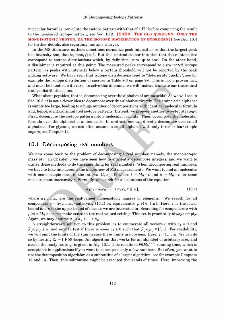
molecular formulas, convolute the isotope pattern with that of a H + before comparing the resultto the measured isotope pattern, see Sec. 10.2. [TODO: THE OLD QUESTION: ONLY THEMONOISOTOPIC PROTON, OR THE ISOTOPE DISTRIBUTION OF HYDROGEN?] See Sec. 10.4for further details, also regarding multiple charges.

In the MS literature, authors sometimes normalize peak intensities so that the largest peakhas intensity one, that is, maxi f i = 1. But this contradicts our intuition that these intensitiescorrespond to isotope distributions which, by definition, sum up to one. On the other hand,a disclaimer is required at this point: The measured peaks correspond to a truncated isotopepattern, as peaks with intensity below a certain threshold will not be reported by the peakpicking software. We have seen that isotope distributions tend to “deteriorate quickly”, see forexample the isotope distribution of sucrose in Table 9.3 on page 99. This is not a proven fact,and must be handled with care. To solve this dilemma, we will instead truncate our theoreticalisotope distributions, too.

What about peptides, that is, decomposing over the alphabet of amino acids? As we will see inSec. 10.6, it is not a clever idea to decompose over this alphabet directly. The amino acid alphabetis simply too large, leading to a huge number of decompositions with identical molecular formulaand, hence, identical simulated isotope patterns. Instead, we propose another two-step strategy:First, decompose the isotope pattern into a molecular formula. Then, decompose the molecularformula over the alphabet of amino acids. In contrast, one can directly decompose over smallalphabets: For glycans, we can often assume a small alphabet with only three or four simplesugars, see Chapter 14.

10.1 Decomposing real numbers

We now come back to the problem of decomposing a real number, namely, the monoisotopicmass M0. In Chapter 3 we have seen how to efficiently decompose integers, and we want toutilize these methods to do the same thing for real numbers. When decomposing real numbers,we have to take into account the inaccuracy of MS measurements: We want to find all moleculeswith monoisotopic mass in the interval [l,u] ⊆ R where l := M0 − ε and u := M0 + ε for somemeasurement inaccuracy ε. Formally, we search for all solutions of the equation

a1c1 +a2c2 +·· ·+ancn ∈ [l,u], (10.1)

where a1, . . . ,an are the real-valued monoisotopic masses of elements. We search for allcompomers c = (c1, . . . , cn) satisfying (10.1) or, equivalently, µ(c) ∈ [l,u]. Here, l is the lowerbound and u is the upper bound of masses we are interested in. Searching for compomers c withµ(c) = M0 does not make sense in the real-valued setting: This set is practically always empty.Again, we may assume a1 < a2 < ·· · < an.

A straightforward solution to this problem, is to enumerate all vectors c with c1 = 0 and∑j a j c j ≤ u, and next to test if there is some c1 ≥ 0 such that

∑j a j c j ∈ [l,u]. For readability,

we will omit the limits of the sum in case these limits are obvious: Here, j = 1, . . . ,k. We can doso by nesting |Σ|−1 FOR-loops. An algorithm that works for an alphabet of arbitrary size, andavoids the nasty nesting, is given in Alg. 10.1. This results in Θ(M0

k−1) running time, which isacceptable in applications if you want to decompose only a few numbers. But often, you want touse the decomposition algorithm as a subroutine of a larger algorithm, see for example Chapters13 and 14. Then, this subroutine might be executed thousands of times. Here, improving the

112

DRAFT


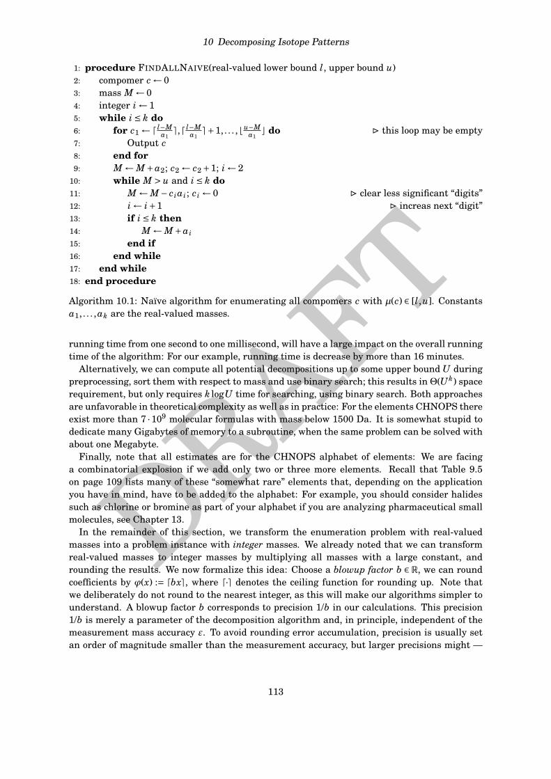
1: procedure FINDALLNAIVE(real-valued lower bound l, upper bound u)2: compomer c ← 03: mass M ← 04: integer i ← 15: while i ≤ k do6: for c1 ←d l−M

a1e,d l−M

a1e+1, . . . ,b u−M

a1c do . this loop may be empty

7: Output c8: end for9: M ← M+a2; c2 ← c2 +1; i ← 2

10: while M > u and i ≤ k do11: M ← M− ciai; ci ← 0 . clear less significant “digits”12: i ← i+1 . increas next “digit”13: if i ≤ k then14: M ← M+ai15: end if16: end while17: end while18: end procedure

Algorithm 10.1: Naïve algorithm for enumerating all compomers c with µ(c) ∈ [l,u]. Constantsa1, . . . ,ak are the real-valued masses.

running time from one second to one millisecond, will have a large impact on the overall runningtime of the algorithm: For our example, running time is decrease by more than 16 minutes.

Alternatively, we can compute all potential decompositions up to some upper bound U duringpreprocessing, sort them with respect to mass and use binary search; this results in Θ(Uk) spacerequirement, but only requires k logU time for searching, using binary search. Both approachesare unfavorable in theoretical complexity as well as in practice: For the elements CHNOPS thereexist more than 7 ·109 molecular formulas with mass below 1500 Da. It is somewhat stupid todedicate many Gigabytes of memory to a subroutine, when the same problem can be solved withabout one Megabyte.

Finally, note that all estimates are for the CHNOPS alphabet of elements: We are facinga combinatorial explosion if we add only two or three more elements. Recall that Table 9.5on page 109 lists many of these “somewhat rare” elements that, depending on the applicationyou have in mind, have to be added to the alphabet: For example, you should consider halidessuch as chlorine or bromine as part of your alphabet if you are analyzing pharmaceutical smallmolecules, see Chapter 13.

In the remainder of this section, we transform the enumeration problem with real-valuedmasses into a problem instance with integer masses. We already noted that we can transformreal-valued masses to integer masses by multiplying all masses with a large constant, androunding the results. We now formalize this idea: Choose a blowup factor b ∈ R, we can roundcoefficients by ϕ(x) := dbxe, where d·e denotes the ceiling function for rounding up. Note thatwe deliberately do not round to the nearest integer, as this will make our algorithms simpler tounderstand. A blowup factor b corresponds to precision 1/b in our calculations. This precision1/b is merely a parameter of the decomposition algorithm and, in principle, independent of themeasurement mass accuracy ε. To avoid rounding error accumulation, precision is usually setan order of magnitude smaller than the measurement accuracy, but larger precisions might —

113

DRAFT


somewhat counterintuitively — result in decreased running times. We will come back to thisissue at the end of the section.

We transform all real-valued masses a1, . . . ,ak into integer masses a′i :=ϕ(ai)= dbaie, and we

also calculate integer bounds l′ := ϕ(l) and u′ := ϕ(u). We want to find all compomers c withµ′(c) ∈ [l′,u′] over the integer alphabet Σ = a′

1, . . . ,a′k, where µ denotes the weighting function

for integer weights. This can be achieved by iterating M = l′, . . . ,u′ and enumerating all c withµ′(c)= M for each M. In Sec. 3.5 and 3.6, we have presented two methods for efficiently solvingsuch instances.

Does this already solve our problem? Obviously not: certain solutions c of the integer massinstance are no solutions of the real-valued mass instance, and vice versa. In other words, theremight be compomers c with integer mass µ′(c) ∈ [l′,u′] but real-valued mass µ(c) ∉ [l,u]. Theseare false positive solutions (see Chapter 5) as we would wrongly report them when solving theinteger instance. We can easily sort out false positive solutions by checking (10.1) for everydecomposition c, resulting in additional running time. On the other hand, there might becompomers c with integer mass µ′(c) ∉ [l′,u′] but real-valued mass µ(c) ∈ [l,u]. These are falsenegative solutions as we would wrongly omit them when solving the integer instance. We nowconcentrate on the more intriguing problem of false negative solutions.

Clearly,∑

j a j c j ≥ l implies∑

j a′j c j ≥ l and, since all a′

j are integer, also∑

j a′j c j ≥ l′. This

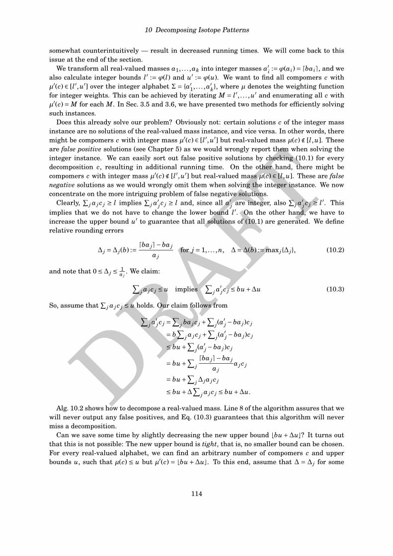
implies that we do not have to change the lower bound l′. On the other hand, we have toincrease the upper bound u′ to guarantee that all solutions of (10.1) are generated. We definerelative rounding errors

∆ j =∆ j(b) := dba je−ba j

a jfor j = 1, . . . ,n, ∆=∆(b) :=max j∆ j, (10.2)

and note that 0≤∆ j ≤ 1a j

. We claim:∑j a j c j ≤ u implies

∑j a′

j c j ≤ bu+∆u (10.3)

So, assume that∑

j a j c j ≤ u holds. Our claim follows from∑j a′

j c j =∑

j ba j c j +∑

j(a′j −ba j)c j

= b∑

j a j c j +∑

j(a′j −ba j)c j

≤ bu+∑j(a

′j −ba j)c j

= bu+∑jdba je−ba j

a ja j c j

= bu+∑j∆ ja j c j

≤ bu+∆∑j a j c j ≤ bu+∆u.

Alg. 10.2 shows how to decompose a real-valued mass. Line 8 of the algorithm assures that wewill never output any false positives, and Eq. (10.3) guarantees that this algorithm will nevermiss a decomposition.

Can we save some time by slightly decreasing the new upper bound bbu+∆uc? It turns outthat this is not possible: The new upper bound is tight, that is, no smaller bound can be chosen.For every real-valued alphabet, we can find an arbitrary number of compomers c and upperbounds u, such that µ(c) ≤ u but µ′(c) = bbu+∆uc. To this end, assume that ∆ = ∆ j for some

114

DRAFT


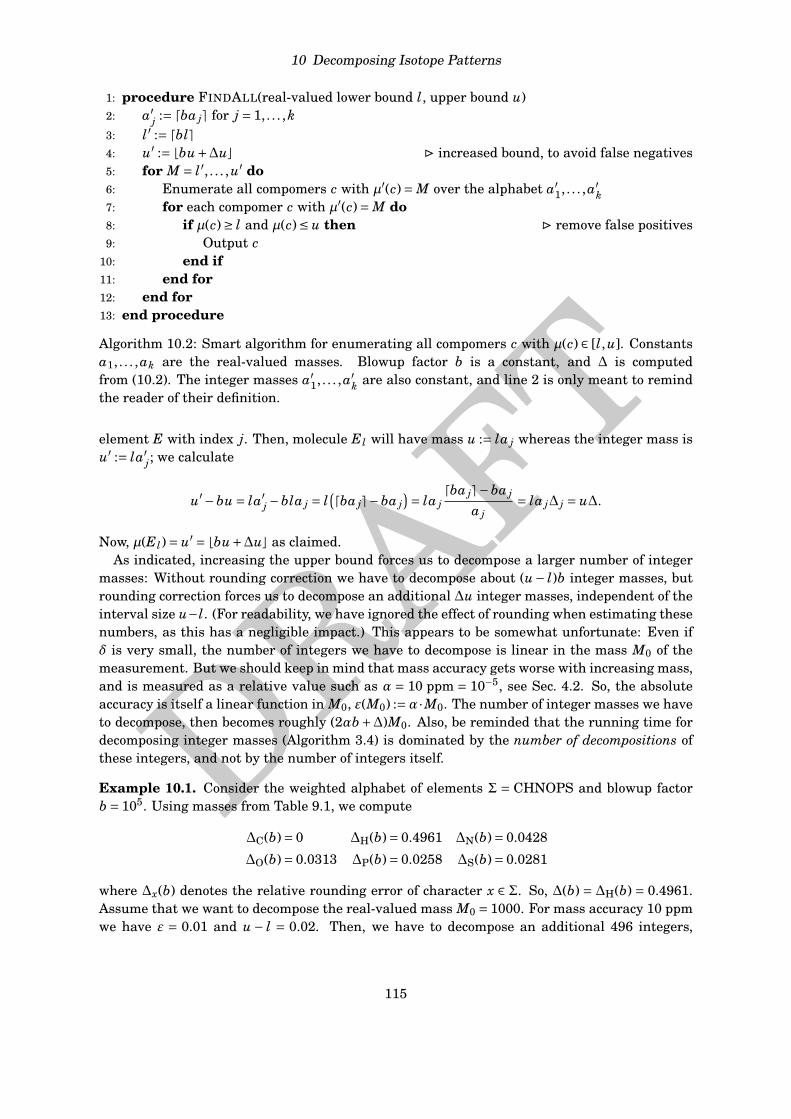
1: procedure FINDALL(real-valued lower bound l, upper bound u)2: a′

j := dba je for j = 1, . . . ,k3: l′ := dble4: u′ := bbu+∆uc . increased bound, to avoid false negatives5: for M = l′, . . . ,u′ do6: Enumerate all compomers c with µ′(c)= M over the alphabet a′

1, . . . ,a′k

7: for each compomer c with µ′(c)= M do8: if µ(c)≥ l and µ(c)≤ u then . remove false positives9: Output c

10: end if11: end for12: end for13: end procedure

Algorithm 10.2: Smart algorithm for enumerating all compomers c with µ(c) ∈ [l,u]. Constantsa1, . . . ,ak are the real-valued masses. Blowup factor b is a constant, and ∆ is computedfrom (10.2). The integer masses a′

1, . . . ,a′k are also constant, and line 2 is only meant to remind

the reader of their definition.

element E with index j. Then, molecule E l will have mass u := la j whereas the integer mass isu′ := la′

j; we calculate

u′−bu = la′j −bla j = l

(dba je−ba j)= la j

dba je−ba j

a j= la j∆ j = u∆.

Now, µ(E l)= u′ = bbu+∆uc as claimed.As indicated, increasing the upper bound forces us to decompose a larger number of integer

masses: Without rounding correction we have to decompose about (u− l)b integer masses, butrounding correction forces us to decompose an additional ∆u integer masses, independent of theinterval size u−l. (For readability, we have ignored the effect of rounding when estimating thesenumbers, as this has a negligible impact.) This appears to be somewhat unfortunate: Even ifδ is very small, the number of integers we have to decompose is linear in the mass M0 of themeasurement. But we should keep in mind that mass accuracy gets worse with increasing mass,and is measured as a relative value such as α = 10 ppm = 10−5, see Sec. 4.2. So, the absoluteaccuracy is itself a linear function in M0, ε(M0) :=α ·M0. The number of integer masses we haveto decompose, then becomes roughly (2αb+∆)M0. Also, be reminded that the running time fordecomposing integer masses (Algorithm 3.4) is dominated by the number of decompositions ofthese integers, and not by the number of integers itself.

Example 10.1. Consider the weighted alphabet of elements Σ = CHNOPS and blowup factorb = 105. Using masses from Table 9.1, we compute

∆C(b)= 0 ∆H(b)= 0.4961 ∆N(b)= 0.0428

∆O(b)= 0.0313 ∆P(b)= 0.0258 ∆S(b)= 0.0281

where ∆x(b) denotes the relative rounding error of character x ∈ Σ. So, ∆(b) = ∆H(b) = 0.4961.Assume that we want to decompose the real-valued mass M0 = 1000. For mass accuracy 10 ppmwe have ε = 0.01 and u − l = 0.02. Then, we have to decompose an additional 496 integers,

115

DRAFT


independent of the mass accuracy. We calculate l′ = 99999000 and u′ = 100001000. In total, wehave to decompose 2497 integer masses, instead of 2001 without correction.

Algorithm 10.2 tells us how to decompose any interval of real numbers; the only parameterof this approach that we have not considered, is the blowup factor b. Be reminded thatindependent of the choice of b, Algorithm 10.2 will never miss a molecular formulas, or producea false positive. In application, you would choose b “reasonable”: It should not be too small,taking into account the anticipated mass accuracy of the instrument. Otherwise, many integerdecompositions will be computed in vain, and have to be discarded by line 8 of the algorithm. Onthe other hand, it should not be too large: Even though computers have Gigabytes of memorythese days, accessing this memory is significantly slower than accessing the processor cache,just like accessing the hard disk is significantly slower than accessing the internal memory. Inapplication, a comparatively small b appears to be a good choice, so that the Extended ResidueTable of Algorithm 3.4 uses less than one Megabyte of memory; recall that the size of this tableis O(kdba1e). For decomposing molecular formulas, b = 5 ·104 is quite reasonable [29].

We will now look at “good choices” for parameter b: Such blowup factors will result in asmall quotient ∆(b)/b of additional integers we have to decompose. Note that we write ∆(b)here, to stress that ∆ actually depends on the chosen blowup. We have to decompose a total of(2αb+∆(b))M0 integer masses, and ∆(b)M0 of these are decomposed because of our roundingtechnique. We want to minimize the relative number of integers that have to be decomposed inaddition, being

∆(b)M0(2αb+∆(b)

)M0

= ∆(b)2αb+∆(b)

, (10.4)

and this number is minimum if ∆(b)/b is minimum. You can easily see this if you try to maximizethe (multiplicative) inverse of (10.4).

See, for example, Example 10.1: Choosing b = 105 seems to be a bad idea as ∆H À ∆x forx ∈ C,N,O,P,S. It turns out that for the alphabet CHNOPS, choosing an optimal blowup factorhas a rather negligible impact on running times [29]. Still, the impact might be significant forother applications.

Suppose that memory considerations imply a maximum blowup factor of B ∈ R. We wantto find b ∈ (0,B] such that ∆(b)/b is minimized. We can explicitly find an optimal such b byconstructing the piecewise linear functions ∆ j(b) := 1

a j(dba je − ba j) with da jBe + 1 sampling

points, for all j = 1, . . . ,k. Next, we set ϕ1 ≡ ∆1 and for j ≥ 2, we define ϕ j as the maximumof ϕ j−1 and ∆ j, a piecewise linear function with O

((a1+·· ·+a j)B

)sampling points. Then, ∆≡ϕk

is a piecewise linear function with O((a1 + ·· · + ak)B

)sampling points. We can construct ∆ in

time O(k(a1 +·· ·+ak)B)=O(k2akB). For every piecewise linear part I ⊆R of ∆ the minimum of∆(b)/b must be located at the terminal points, so it suffices to test the O(kakB) sampling pointsof ∆ to find the minimum of ∆(b)/b.

10.2 Evaluating molecular formulas

Now that we have filtered down to a few (possibly, still tens of thousands of) molecular formulas,we want to evaluate them, as proposed in Sec. 8.4. Here, our advantage is that we do not onlyknow something about the presence or absence of certain peaks — in fact, isotope patterns arerater boring with this respect, as all of them contain a string of peaks at about one Daltondistance — but we also have a clear idea of the masses and intensities of these peaks. Note that

116

DRAFT


matching peak pairs between the measured spectrum and each reference spectrum is mostlytrivial, because in both cases we have a string of peaks mentioned above. The only possibleexception is sulfur and other “maverick” elements, see below.

A particularly important aspect that we have to consider in this section, is speed: As notedabove, we might evaluate ten thousands of candidates for a single isotope pattern; and ourMS measurement may contain ten thousands of such patterns. So, it makes a difference if wespeed up our evaluation algorithm from 1 milisecond to 0.1 miliseconds, to evaluate a candidatemolecular formula.

As we have a precise idea of what our measured spectrum should look like, given that somereference spectrum is the correct explanation, we do not use a general scoring schemes, seeSec. 4.2. Instead, we build a “custom-made” scoring, as suggested in Sec. 4.5. We want to useBayesian Statistics to evaluate mass spectra matches:

P(Mi|D,B)= P(Mi|B) ·P(D|Mi,B)∑iP(Mi|B)P(D|Mi,B)

(10.5)

where D is the data (the measured spectrum), Mi are the models (the candidate molecules), andB stands for any prior background information. Probabilities P(Mi|D,B) are called posteriorprobabilities, whereas P(D|Mi,B) are conditional probabilities. At the end of our analysis, wewill sort molecular formulas (i.e. the models) with respect to posterior probabilities P(Mi|D,B),and choose the one with highest posterior probability as the most likely explanation of the data.

Eq. 10.5 is an example of a naïve Bayes classifier, and such classifiers have been successfullyused for numerous applications, we mention “spam filtering” as a prominent example. Eq. 10.5allows us to compute the probability of each model (given the data), using the probability of thedata, given each model.

What does “background information” mean? This is anything we know about molecular for-mulas without looking at the data: For example, certain molecular formulas such as H200 cannotcorrespond to an actual molecules. We will come back to this issue in the next section; for themoment, we set the prior probability P(Mi|B) to zero for all molecules but the decompositionsof the monoisotopic mass, and assume that all decompositions have identical prior probability.Note that we have slightly stretched the definition, by including the monoisotopic mass in thebackground information.

We now iterate over all models, and concentrate on a particular model M as our candidatemolecular formula. As we will see in Sec. 10.4, there is only one thing left for us to compute: Thisis the conditional probability P(D|M ,B), the probability of the data given the model. To computethis probability, we have to make some assumptions regarding independence: We assume thatfor each peak, the random mass error is independent of other peaks’ mass errors as well asintensities; for each peak, we assume that the random intensity error is independent of otherpeaks’ intensity errors as well as masses; and, we assume that both are independent from thebackground information. These are quite reasonable assumptions (compare to Sec. 4.2) withthree exceptions:

1. As noted in Sec. 4.2, mass errors also have a systematic component.

2. One can observe that mass errors get larger as peak intensities get smaller; for smallpeaks that are almost “lost in the noise”, it gets much harder for the peak picking softwareto pick the correct mass.

3. Obviously, peak intensities are correlated, as all peak intensities have to sum up to one.

117

DRAFT


The first problem will, at least in part, be addressed below; the second can be easily addressed;but there appears to be no simple way to deal with the last. Still and all, we assumeindependence, so that we can swiftly calculate a conditional probability estimate. We reach:

P(D|M ,B)=nmax∏j=0

P(M j|m j) ·nmax∏j=0

P( f j|p j). (10.6)

Here, P(M j|m j) is the probability to observe peak j at mass M j when, according to model M ,its true mass is m j; and P( f j|p j) is the probability to observe peak j with intensity f j when,according to the model, its true intensity is p j.

Scoring peak masses is pretty much done as described in Sec. 4.2, we swiftly recall the details.As noted there, the mass error is roughly normally distributed with mean zero. The massaccuracy α of the instrument is given as a parameter, such as α = 10 ppm = 10−5. We assumea standard deviation of σmass := 1

3αM0 for peak masses, assuming that more than 99.7% ofmeasurements fall into the specified mass range. Note that measured masses M0, . . . , Mnmax areso similiar, that one standard deviation should do the job. One can also take into account thatweak peaks have worse mass accuracy then strong peaks, using an individual mass accuracy foreach peak; we omit the details. We estimate the probability that of observing a mass differenceof

∣∣M j −m j∣∣ or larger as:

P(M j|m j)= erfc( ∣∣M j −m j

∣∣p

2σmass

)= 2p

2π

∫ ∞

ze−t2/2dt (10.7)

with z := |M j−m j|σmass

, for j = 0, . . . ,nmax. Compare to (4.5) on page 63.But even for MS with high mass accuracy, spectra can show a systematic mass shift due to

calibration inaccuracies. We can easily eliminate this shift for all masses but the monoisotopicmass: We do not compare masses of the +1,+2, . . . peaks directly but instead, difference to themonoisotopic peak, M j −M0 vs. m j −m0:

P(M j|m j)= erfc( ∣∣M j −M0 −m j +m0

∣∣p

2σmass

)(10.8)

for j = 1, . . . ,nmax. Note that P(M0|m0) is still computed using (10.7) directly. Recall fromExercise 4.6 that from a mathematical standpoint, we would have to assume an increasedstandard deviation of

p2σmass; but from an MS perspective, we should rather stick with

standard deviation σmass, as the difference between the masses is very small.Different from mass inaccuracies, much less is known about the distribution of intensity

inaccuracies. For the sake of simplicity, we assume that intensity errors are also normallydistributed; this will allow us to swiftly compute the required probabilities for (10.6). Butdifferent from mass errors, we will not use absolute intensity errors in our computations, butinstead intensity ratios: If a peak is twice as high as we expect it too be, that is a bad thing,even if the absolute error is small. So, let us assume that log ratios between measured andpredicted peak intensity log( f j/p j) follow a normal distribution. What we want to calculate, isthe probability that an intensity ratio “at least as lopsided” as the one we have recorded, mightcome up by chance: Set r := max f j/p j, p j/ f j ≥ 1, then we want to estimate the probability thata intensity ratio outside the interval [1/r, r] occurs by chance.

We assume that a “intensity precision parameter” β is provided by the user; for example,β= 10% means that we expect 99.7% of all intensity ratios to fall into the range [ 1

1+β ,1+β] or,

118

DRAFT


equivalently, that 99.7% of all log intensity ratios fall into the range [− log(1+β), log(1+β)]. Weset σint := 1

3β. Analogously to (10.7), we estimate the probability of observing a peak intensityratio at least as lopsided as the one we have observed, as:

P( f j|p j)= erfc( ∣∣log( f j/p j)

∣∣p

2σint

)= 2p

2π

∫ ∞

ze−t2/2dt (10.9)

with z := |log( f j /p j)|σint

, for j = 0, . . . ,nmax.This concludes our calculation of the conditional probability P(D|M ,B); the missing prior

probability P(M |B) is covered in the next section.

10.3 Integrating chemical knowledge

We will now take a closer look at chemical restrictions for the molecular formulas we aregenerating: These should correspond to some molecular, after all. It turns out that molecularformulas that can be found in databases such as PubChem, follow certain rules which can beused to filter out those that are “very unlikely”. Here, we propose a different approach: As wehave generated all molecular formulas anyways, there is no need for setting a hard threshold.Instead, molecular formulas that are somewhat unlike because of their “abnormal” composition,will simply be penalized through the prior probability. In the following, we are looking at themolecular formula of the neutral molecule, not at the molecular formula of the ion.

First, let us have a look at the molecule graph of the unknown molecule: This graph should beconnected, so that we are truly looking at a single molecule. We also assign prior probability zeroto molecular formulas that cannot correspond to a molecule, because of chemical considerations:Senior’s third theorem states that the sum of valences has to be greater than or equal to twicethe number of atoms minus one [207]. Molecules violating Seniors third theorem are rare,particularly for natural compounds: less than 0.16% of substances in the KEGG COMPOUNDdatabase [124] (again release 42.0) violate this rule. We also filter out radicals with odd sum ofvalences.

List further rules from Kind and Fiehn [137], warning: this might rather reproduce what isalready known.

Here comes the next warning: We must not use the empirical distributions of, say, the hetero-to-carbon ratio directly, in order to compute a prior probability. These “distributions” onlydescribe what is found in some molecule databases. There is no information attached to thatdatabase how frequently each particular molecular formula is found in an MS experiment; inparticular, there is no information in there about the experiment that you are analyzing. Itmight be that certain hetero-to-carbon ratios are quite common in the database, whereas thecorresponding molecules are extremely rare in experiments. It might also be that you are lookingat a particular class of biomolecules that has hetero-to-carbon ratios quite different from whatyou find in databases.

We want to circumvent these problems but, at the same time, we want to use the fact thatcertain hetero-to-carbon ratios are extremely rare. For this, I propose a heuristic approach thathas no formal justification, besides the fact that it makes some sense, in the “common sense”meaning of the word. Let us, again, concentrate on hetero-to-carbon ratios. Assume that 99.9%of the molecules in the databases have hetero-to-carbon ratio in the interval [a,b], only 0.05%have a ratio smaller than a, and only 0.05% have a ratio larger than b: These molecules shouldnot be affected by the prior, as apparently, there is quite a large number of molecules that have

119

DRAFT


hetero-to-carbon ratios being even more lopsided. Assume that only 0.005% of the moleculeshave a ratio below a′, and only 0.005% have a ratio above b′: These molecules are somewhat“too lopsided”, but molecular formulas with such a ratio can quite possibly still be true. Let

f (x) := exp(−12 x2)

be the Gaussian function,1 and note that f (0) = 1 and f (±p8ln2) = 12 . Now, build a function g

as follows:

g(x) :=

f(

x−ap8ln2·(a−a′)

)for x ≤ a

1 for a < x < b

f(

x−bp8ln2·(b′−b)

)for x ≥ b

(10.10)

One can easily check that this is a continuous function, and that

g(a′)= f(−(a−a′)/

p8ln2(a−a′)

)= f (−p

8ln2)= 12

and, similarly, g(b′)= 12 .

Pellegrin [185][TODO: RADICALS? OTHER SENIOR’S THEOREM?]

10.4 Wrapping it up

We have almost everything in place to “decompose” isotope patterns: We can decompose themonoisotopic mass; for a candidate molecular formula, we can easily simulate its isotopepattern; we can evaluate the simulated isotope pattern using Bayesian statistics; and, we knowhow to estimate prior probabilities for each candidate molecular formula. But what about thedenominator

∑iP(Mi|B) ·P(D|Mi,B) in (10.5)? It turns out that we do not have to compute this

sum, the reason being as follows: Let M1, . . . ,Ml be the models (candidate molecular formulas)to choose from. Then,

l∑i=1

P(Mi|D,B)= 1

must hold: As we have no other models that might explain the data, one of them must be true,and their posterior probabilities must sum to one. But this means that we can simply normalizethe products P(Mi|B) ·P(D|Mi,B) we have calculated for the different models: Let

c :=l∑

i=1P(Mi|B) ·P(D|Mi,B)

then∑

iP(Mi|B) ·P(D|Mi,B)= 1/c must hold.In the introduction of this chapter, we suggested the following analysis procedure: Assume

that your molecular ion carries a certain adduct ion, such as H +, sodium Na +, or potassium K +.Then, subtract the proton mass before applying the mass decomposition algorithm; and for allcandidate molecular formulas, convolute the isotope pattern with that of the adduct ion beforecomparing the result to the measured isotope pattern. If you do not know the correct adduct ion,then repeat the analysis for all potential adduct ions, and output the pair (molecular formula,

120

DRAFT


1: procedure DIP(intensities f0, . . . , fnmax , masses M0, . . . , Mnmax , set A )2: Init psum ← 03: Empty list L

4: for each adduct ion a ∈A do5: M ← f0 −µ(a) . monoisotopic mass of adduct6: l ← M−αM; r ← M+αM . mass range to decompose7: FINDALL(l,r) with output C being a list of compomers over Σ8: for each compomer (molecular formula) c ∈C do9: Compute prior probability pprior of c,a

10: Simulate isotope pattern p0, . . . , pnmax and m0, . . . ,mnmax of c+a11: Compute conditional probability pcond of c+a from (10.6)12: Add (c,a, pprior · pcond) to L

13: psum ← psum + pprior · pcond14: end for15: end for16: for each (c,a, p) ∈L do . normalize posterior probabilities17: Replace (c,a, p) by (c,a, p/psum) in L

18: end for19: Sort L with respect to third entry20: end procedure

Algorithm 10.3: Decomposing an isotope pattern f0, . . . , fnmax and M0, . . . , Mnmax of a single-charged ion, where A is the set of potential adduct ions. Additional parameters are the fixedalphabet Σ of elements, the mass function µ : Σ∪A → R, mass accuracy α > 0, and intensityaccuracy β> 0.

adduct ion) that scored best among all adduct ions and all moleular formulas. We have wrappedup things in Algorithm 10.3.

What about multiple charges? As noted in Chapter 7, it is mostly trivial to derive the chargestate from the isotope pattern. Then, subtract “adduct mass times charge state” from themonoisotopic mass; multiply this mass by charge state; decompose the resulting mass; for allcandidate molecular formulas, convolute the simulated isotope pattern with the multiple adductisotope pattern, and devide all masses by the charge state. If you have a set of adduct ions tochoose from, you have to iterate over all combinations of adduct ions. Algorithmically, this issomewhat trivial, but adds another “layer of obscurity” to our algorithms; so, we have ignoredcharge states in Algorithm 10.3 for the ease of presentation.

10.5 On the number of molecular formulas over CHNOPS

The lesson to be learned from the above figures is simple: Even if we have an excellent MSinstrument with mass accuracy 1 ppm or below (recall the difference between “anecdotal massaccuracy” [248] and everyday mass accuracy), the number of decompositions becomes large asmasses exceed 1000 Da — even for the small alphabet of elements CHNOPS. This means that

1I use the Gaussian function here solely because it has certain nice “mathematical properties”; no connection toa Normal distribution is intended or should be assumed. Any similarity to actual persons, living or dead, or toactual events is purely coincidental.

121

DRAFT


we cannot hope to recover the correct molecular formula from monoisotopic mass alone. Intheir 2006 paper “Metabolomic database annotations via query of elemental compositions: Massaccuracy is insufficient even at less than 1 ppm”, Kind and Fiehn [136] also consider chemicalrestrictions and find — well, pretty much what the title suggests.

10.6 Decomposing amino acids

Not a good idea directly, decompose into molecular formula first, then decompose the molecularformula into aa.

[TODO: DESCRIBE WHAT ANTON AND I HAVE DONE.]Note that the number of decompositions will quickly explode, in particular if the mass

accuracy of the instrument is not sufficiently high: For example,

µ(AD)= 186.064057≈ 186.079313=µ(W)

µ(SV)= 186.100442≈ 186.079313=µ(W)

µ(GV)= 156.089878≈ 156.101111=µ(R)

µ(K)= 128.094963≈ 128.058578=µ(Q)

for amino acid residues of alanine A, aspartic acid D, glycine G, lysine K, glutamine Q,arginine R, serine S, valine V, and tryptophan W.

But even if we had an instrument of arbitrary precision, we could not tell apart certaincompomers over the amino acid alphabet, besides the obvious µ(I)=µ(L) ambiguity: For example,µ(AD) = µ(EG), µ(AG) = µ(Q), and µ(GG) = µ(N) holds for additional residues glutamic acid E

and asparagine N. These amino acid residues or combinations thereof have identical molecularformula. So, for mass 840.347442 that may be decomposed into three Q and four N, we canreplace each Q by AD and each N by GG, resulting in 20 decompositions with identical mass.

Fig. 10.2 shows the number of decompositions over the amino acid alphabet, where leucineand isoleucine are treated as a single character. This chart was computed using recurrence (3.2)from page 43, and calculations were carried out with accuracy 10−6 Da.2 Note that the growthis sub-exponential, as an exponential growth would correspond to a straight line. One can learnat least two things from this figure: Firstly, the number of decompositions explodes at 2000 Dalatest, even for instruments with accuracy 1 ppm or better. Second, the combinatorial effects arestill huge at 3000 Da, so the number of decompositions is hard to approximate. [TODO: FILLIN FIGURES, MORE TEXT.]

As we mentioned above, it is not a reasonable approach to decompose large masses in yourmass spectrum over the amino acid alphabet: Clearly, if you are lucky, you will hit a “sweetspot” where only a relatively small number of amino acid decompositions are found. The massspectrometry literature, again, contains many such “anecdotal” decompositions. But we areinterested in fully automated methods that work for all (good quality) input data, not just afew hand-selected peptides. At 2500 Da, we would have to process more than [TODO: 107]decompositions on average, with dreadful consequences for the running time of our method. Youcan decompose, though, the mass difference between two peaks in a mass spectrum, given thatthis difference is at most, say, 1000 Da: In this case, you have to deal with less than [TODO: X]decompositions in the worst case. Both estimates assume a mass accuracy of 1 ppm.

2That is, real-valued masses were multiplied by 106, rounded, and used as integer masses for the recurrence.

122

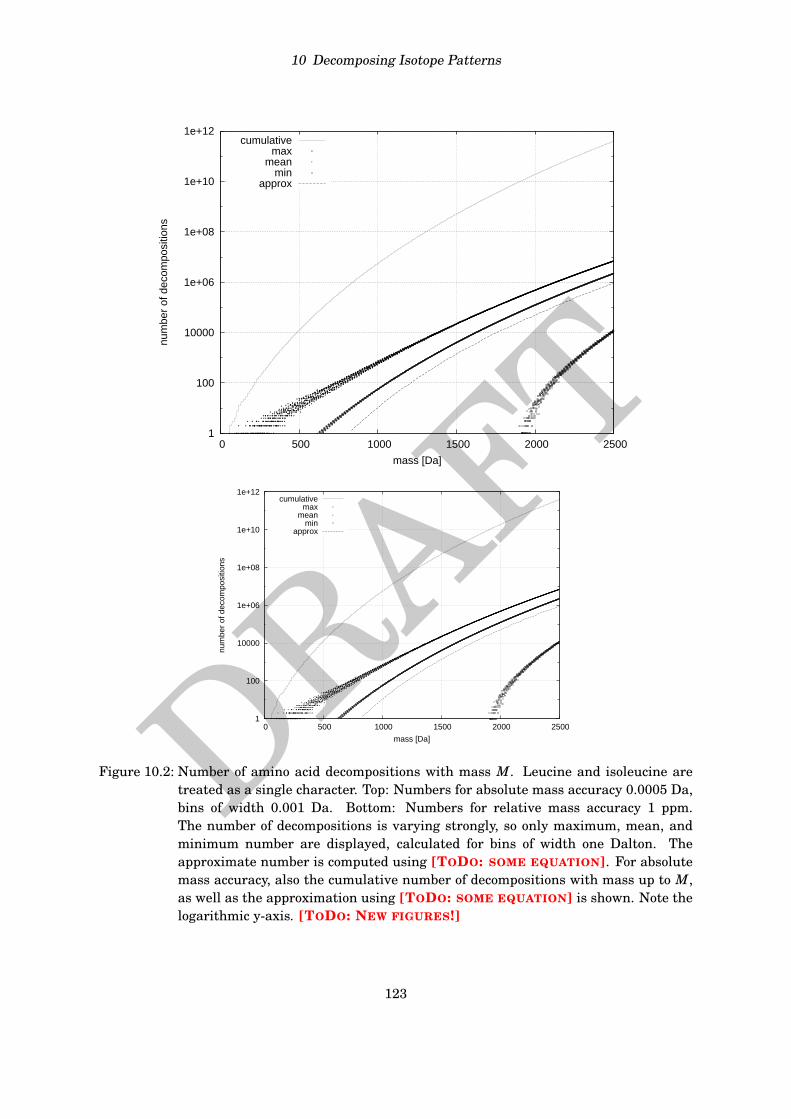
DRAFT


1

100

10000

1e+06

1e+08

1e+10

1e+12

0 500 1000 1500 2000 2500

num

ber

of d

ecom

posi

tions

mass [Da]

cumulativemax

meanmin

approx

1

100

10000

1e+06

1e+08

1e+10

1e+12

0 500 1000 1500 2000 2500

num

ber

of d

ecom

posi

tions

mass [Da]

cumulativemax

meanmin

approx

Figure 10.2: Number of amino acid decompositions with mass M. Leucine and isoleucine aretreated as a single character. Top: Numbers for absolute mass accuracy 0.0005 Da,bins of width 0.001 Da. Bottom: Numbers for relative mass accuracy 1 ppm.The number of decompositions is varying strongly, so only maximum, mean, andminimum number are displayed, calculated for bins of width one Dalton. Theapproximate number is computed using [TODO: SOME EQUATION]. For absolutemass accuracy, also the cumulative number of decompositions with mass up to M,as well as the approximation using [TODO: SOME EQUATION] is shown. Note thelogarithmic y-axis. [TODO: NEW FIGURES!]

123

DRAFT


10.7 Decomposing average masses

We come back to the problem of finding a molecular formula that best explains the observedisotope pattern; but this time, we assume that the monoisotopic peak is lost. This can happenif the molecular formula contains elements that are not frequent in biomolecules, see Table 9.5.For example, the non-proteogenic amino acid C3H7N1O2Se1 has a monoisotopic peak withrelative intensity

0.997573 ·0.999887 ·0.99636 ·0.997572 ·0.0089= 0.0086%.

Clearly, this peak is easily missed by any peak picking software. In contrast, if we stick with theclassical elements CHNOPS then we can usually assume that the monoisotopic peak is present:You need 279 carbon atoms, 24963 hydrogen atoms, 822 nitrogen atoms, 1232 oxygen atoms,or 59 sulfur atoms so that the relative intensity of the monoisotopic peak is below 5%. So, theresulting compound has mass at least 1886 Da if it is made solely from sulfur, mass 3348 Daif it is solely made from carbon, and even higher mass for the other elements. The peptidesof smallest mass where the monoisotopic peak drops below 5%, consist of 34 cysteine residues(mass 3520.323 Da) or 27 methionine residues (mass 3556.104 Da), compare to Exercises 9.5and 9.6 in the previous chapter.

The elements boron,3 iron, selenium, and tungsten have natural isotope distributions that caneasily result in the non-detection of the monoisotopic peak. If you assume that your compoundcontains only few of these atoms with “strange” isotope pattern, then testing each hypothesisindividually might be the best way to go: Assume that the compound contains at most twoiron atoms, and that the first peak of the sample isotope pattern is detected at mass M. Then,decompose masses M, M −µ(Fe), and M −2µ(Fe) as described in Sec. 10.1, add Fe (Fe2) to allcandidates from the second (third) candidate list, respectively, concatenate the lists, and scoreall candidates as described in Sec. 10.2. Note that this approach should not be used for zinc orbromine containing molecules as here, the +1 peak is in fact a mixture of several isotope speciesthat contribute towards its mass.

The mass of the monoisotopic peak is an additive invariant of the decompositions we aresearching for: Given any solution, the sum of monoisotopic masses of all elements is the inputmass M0. In this section, we present other additive invariants for molecules resulting fromthe observed isotope distribution. For the following, we define a weighted alphabet (Σ,µ) as analphabet Σ together with a mass function µ : Σ→N. For simplicity, we often write µ(si) | s ∈ Σfor (Σ,µ). For the alphabet CHNOPS, we have already defined one mass function: µ(E) denotesthe monoisotopic mass of element E. We will now define other mass functions for the samealphabet.

In the rest of this section, we consider a theoretical molecule where iE denotes the multiplicityof element E in the molecule, E ∈Σ. Recall that we can decompose integers only, so we assumein the following that all masses are rounded using appropriate precisions.

Given the observed normalized intensities f0, . . . , fnmax and peak masses M0, . . . , Mnmax , weeasily estimate the average mass of the molecule as Mav :=∑

i f iMi. This will underestimate theaverage mass of the molecule, but this error is superseded by measurement errors. The averagemass of an element E can be estimated by E(XE). Let µ1 denote the corresponding weightfunction; we decompose the number Mav over these weights. [TODO: TURN THE FOLLOWINGINTO EXERCISES!]3The natural isotope abundances of boron differs largely depending on where the sample has been taken, so

particular care is needed if you assume your compound to contain boron.

124

DRAFT


• Intensity of the monoisotopic peak. For every element E, let pE denote the probability thatan isotope of this element is monoisotopic. What is the intensity of the monoisotopic peakof our molecule? Clearly, this is the probability that the molecule has monoisotopic mass,which implies that all atoms must have monoisotopic mass:

p∗ :=P(molecule has monoisotopic mass)= ∏E∈Σ

p iEE (10.11)

Recall that f0 ∈ [0,1] denotes the observed normalized intensity of the monoisotopic peak,so the measurement f0 should agree with p∗; taking the logarithm we find∑

E∈ΣiE · log pE = log f0. (10.12)

Defining a third set of weights for our alphabet, µ2(E) :=− log pE for every element E, wecan decompose the number − log f0 over these weights. Note that by definition, µ2(P) = 0holds for phosphor.

• Relative intensity of the +1 peak. Let qE denote the probability that an isotope of thiselement has nominal mass one above the monoisotopic, for every element E. Note thatqE = 1− pE for E ∈ C,H,N, qE < 1− pE for E ∈ O,S, and qP = 0.

What is the probability that exactly one carbon atom is of isotope type +1, while all otheratoms of our molecule are monoisotopic? One can easily see that this probability is iE

qCpC

p∗,see (10.11) for the definition of p∗. In total, the probability to find exactly one atom of themolecule of isotope type +1 and, hence, the intensity of the +1 peak, is

P(molecule has nominal mass N +1)=∑E∈Σ iE

qEpE

p∗. (10.13)

Recall that f1 ∈ [0,1] denotes the normalized intensity of the +1 peak, then comparison tothe monoisotopic peak leads to the equality:∑

E∈ΣiE · qE

pE= f1

f0(10.14)

Hence, we can define a fourth set of weights for our alphabet, µ3(E) := qE/pE for everyelement E. We can decompose the number f1/ f0 over these weights. Note that againµ3(P)= 0 holds.

• Mass of the +1 peak. Let Y := Y1 + ·· · + Yl be the random variable corresponding toour molecule with monoisotopic nominal mass N. We calculate the difference betweenexpected masses of +1 peak and monoisotopic peak, see (9.3) for the expected mass m1 ofthe +1 peak. Let δE be the mass difference between the +1 mass and monoisotopic massof element E, for example δC = 13.003355−12= 1.003355. For phosphor we define δP := 0.Then,

m1 −m0 = P(Y = N)P(Y = N +1)

∑E∈Σ

iEqE

pEδE, (10.15)

where P(Y = N)= p∗. Recall that M0, M1 denote the observed masses of the monoisotopicand +1 peak. The measured mass difference M1 −M0 should agree with m1 −m0, and inview of P(Y = N +1)= f1 and P(Y = N)= f0, we infer

f1

f0· (M1 −M0)= ∑

E∈ΣiE · qE

pEδE. (10.16)

125

DRAFT


Hence, we can define a fifth set of weights for our alphabet, µ4(E) := qEpEδE for every

element E. We can decompose the number f1f0

(M1−M0) over these weights. Again, µ4(P)= 0holds.

10.8 Historical notes and further reading

Our presentation in this chapter largely follows the paper of Böcker, Letzel, Lipták, andPervukhin [29]. Sec. 10.3 follows Kind and Fiehn [137], with the twist that I have transformedtheir rules into prior probabilities.

Fig. 10.1 is modified from a 2006 publication by Kind and Fiehn [136], where the authorsproposed to build an automated pipeline, similar to the one presented in this chapter.

The idea of assigning molecular formulas to peak masses, dates back at least to the year 1965,when the “Artificial Intelligence” program DENDRAL was created for this task, see Sec. 13.6below.

Using Bayesian Statistics to evaluate mass spectra matches has been suggested by severalauthors, see for example Zhang and Chait [247] and Zhang et al. [246].4

We assumed above that log ratios between measured and predicted peak intensities log( f j/p j),follow a normal distribution. As Böcker et al. [29] note, “our data indicates that after correction,log ratios [. . . ] roughly follow a normal distribution.” This must not be taken as somesort of “truth”, so do not cite me on that issue. More empirical estimations are required toaccept or reject this hypothesis, or estimate the error that we introduce by assuming a normaldistribution. For swift computations, it might still be a good estimate even if the distribution isnot normal.

When computing probabilities from peak intensities, we face another systematic error: In casea peak has low intensity, then this intensity is often under-estimated; the converse is true forpeaks with high intensity [29]. This problem may arise from inaccurate baseline correction, seeSec. 15.2, as such inaccuracies have unequal effects on peaks of different intensities. To improveidentification rates, a correction parameter should be learned from the data.

There exist many other methods for decomposing isotope patterns, but mostly, these methodsare part of commercial and proprietary software, and no details on how these methods workhave been published. See Neumann and Böcker [171] regarding a comparison of the methodpresented here, and the Bruker SmartFormula software. The SmartFormula software imple-ments an approach very similar to the one presented here, but is said to use χ2 statistics toscore the molecular formulas — but this statistics is for a small number of observations, and notmeant to differentiate between a set hypotheses.

Several programs are available to decompose masses over the amino acid alphabet; mostprograms rely on the naïve approach for decomposing masses as presented in Sec. 10.1 and haveto somewhat arbitrarily restrict the search space, by introducing upper bounds on the numberof certain amino acids, to avoid the combinatorial explosion.

[TODO: LOOK AT [84, 96, 113]][189] do it for oligonucleotides.Rogers, Scheltema, Girolami, and Breitling [198] propose a quite different approach to assign

molecular formulas to metabolites: Instead of treating each measurement individually, theyassign molecular formulas to a batch of metabolite masses. Here, they use the fact that

4Wenzhu Zhang for [247] and Ning Zhang for [246].

126

DRAFT


metabolites are connected to each other via chemical transformations [32]. They then use Gibbssampling to find a model with maximum posterior probability, given the data.

[TODO: ZUBAREV AND MANN [248] SAY SOMETHING ABOUT 1 PPM MASS ACCURACY ISENOUGH — COMMENT, THEY DO DB SEARCH, WE DO DE NOVO.]

Zhang et al. [245]As a successful example for an automated method that decomposes masses over the amino

acid alphabet, we mention the approach of Bertsch et al. [18] who use such decompositions aspart of a divide-and-conquer strategy.

10.9 Exercises

10.1 "Uber realen Massen zerlegen: Gegeben sei das Alphabet H,C, N,O mit den Massen1.008,12.0,14.003,15.995. Beschreibe einen naiven Algorithmus (ohne Verwendung vonFKR), der alle Zerlegungen f"ur eine gegebene Masse M und eine Abweichung ε berechnet.Berechne alle Zerlegungen f"ur die Masse 100 und die Abweichung 0.01. Wie viele gibt es?

10.2 Similar to Exercise 10.2, it is easy to modidify Algorithms 10.1 and 10.2, when upper andlower bounds for each character are given. Show how this can be done.

127

DRAFT

Bibliography

[1] A. Aaant. I need a title, quick. [TODO: REPLACE WITH A REAL CITATION], 2101.

[2] G. Alves, A. Y. Ogurtsov and Y.-K. Yu. RAId_DbS: peptide identification using databasesearches with realistic statistics. Biol. Direct., 2:25, 2007.

[3] S. Andreotti, G. W. Klau and K. Reinert. Antilope – a lagrangian relaxation approach tothe de novo peptide sequencing problem. IEEE/ACM Trans. Comput. Biol. Bioinform.,2011. To appear, doi:10.1109/TCBB.2011.59.

[4] R. Apweiler, H. Hermjakob and N. Sharon. On the frequency of protein glycosylation, asdeduced from analysis of the SWISS-PROT database. Biochim. Biophys. Acta, 1473(1):4–8, 1999.

[5] G. Audi, A. Wapstra and C. Thibault. The AME2003 atomic mass evaluation (ii): Tables,graphs, and references. Nucl. Phys. A, 729:129–336, 2003.

[6] J.-M. Autebert, J. Berstel and L. Boasson. Context-free languages and pushdown au-tomata. In G. Rozenberg and A. Salomaa, editors, Handbook of Formal Languages,volume 1, pages 111–174. Springer, 1997.

[7] V. Bafna and N. Edwards. SCOPE: A probabilistic model for scoring tandem mass spectraagainst a peptide database. Bioinformatics, 17:S13–S21, 2001.

[8] D. A. Barkauskas and D. M. Rocke. A general-purpose baseline estimation algorithm forspectroscopic data. Anal. Chim. Acta, 657(2):191–197, 2010.

[9] C. Bartels. Fast algorithm for peptide sequencing by mass spectrometry. Biomed. Environ.Mass Spectrom., 19:363–368, 1990.

[10] J. M. S. Bartlett and D. Stirling. A short history of the polymerase chain reaction. MethodsMol. Biol., 226:3–6, 2003.

[11] C. Bauer, R. Cramer and J. Schuchhardt. Evaluation of peak-picking algorithms forprotein mass spectrometry. Methods Mol. Biol., 696:341–352, 2011.

[12] M. Beck, I. M. Gessel and T. Komatsu. The polynomial part of a restricted partitionfunction related to the Frobenius problem. Electron. J. Comb., 8(1):N7, 2001.

[13] D. E. Beihoffer, J. Hendry, A. Nijenhuis and S. Wagon. Faster algorithms for Frobeniusnumbers. Electron. J. Comb., 12:R27, 2005.

[14] C. Benecke, T. Grüner, A. Kerber, R. Laue and T. Wieland. MOLecular StructureGENeration with MOLGEN, new features and future developments. Anal. Chim. Acta,314:141–147, 1995.

177

DRAFT

Bibliography

[15] G. Benson. Composition alignment. In Proc. of Workshop on Algorithms in Bioinformatics(WABI 2003), volume 2812 of Lect. Notes Comput. Sc., pages 447–461. Springer, 2003.

[16] M. W. Bern and D. Goldberg. EigenMS: De novo analysis of peptide tandem mass spectraby spectral graph partitioning. In Proc. of Research in Computational Molecular Biology(RECOMB 2005), volume 3500 of Lect. Notes Comput. Sc., pages 357–372. Springer, 2005.

[17] M. W. Bern and D. Goldberg. De novo analysis of peptide tandem mass spectra by spectralgraph partitioning. J. Comput. Biol., 13(2):364–378, 2006.

[18] A. Bertsch, A. Leinenbach, A. Pervukhin, M. Lubeck, R. Hartmer, C. Baessmann, Y. A.Elnakady, R. Müller, S. Böcker, C. G. Huber, and O. Kohlbacher. De novo peptidesequencing by tandem MS using complementary CID and electron transfer dissociation.Electrophoresis, 30(21):3736–3747, 2009.

[19] K. Biemann, C. Cone and B. R. Webster. Computer-aided interpretation of high-resolutionmass spectra. II. Amino acid sequence of peptides. J. Am. Chem. Soc., 88(11):2597–2598,1966.

[20] K. Biemann, C. Cone, B. R. Webster and G. P. Arsenault. Determination of the aminoacid sequence in oligopeptides by computer interpretation of their high-resolution massspectra. J. Am. Chem. Soc., 88(23):5598–5606, 1966.

[21] A. Björklund, T. Husfeldt, P. Kaski and M. Koivisto. Fourier meets Möbius: fast subsetconvolution. In Proc. of ACM Symposium on Theory of Computing (STOC 2007), pages67–74. ACM Press New York, 2007.

[22] N. Blow. Glycobiology: A spoonful of sugar. Nature, 457(7229):617–620, 2009.

[23] S. Böcker. Sequencing from compomers: Using mass spectrometry for DNA de-novosequencing of 200+ nt. J. Comput. Biol., 11(6):1110–1134, 2004.

[24] S. Böcker and Zs. Lipták. A fast and simple algorithm for the Money Changing Problem.Algorithmica, 48(4):413–432, 2007.

[25] S. Böcker and V. Mäkinen. Combinatorial approaches for mass spectra recalibration.IEEE/ACM Trans. Comput. Biol. Bioinform., 5(1):91–100, 2008.

[26] S. Böcker and F. Rasche. Towards de novo identification of metabolites by analyzingtandem mass spectra. Bioinformatics, 24:I49–I55, 2008. Proc. of European Conferenceon Computational Biology (ECCB 2008).

[27] S. Böcker, M. Letzel, Zs. Lipták and A. Pervukhin. Decomposing metabolomic isotopepatterns. In Proc. of Workshop on Algorithms in Bioinformatics (WABI 2006), volume4175 of Lect. Notes Comput. Sc., pages 12–23. Springer, 2006.

[28] S. Böcker, B. Kehr and F. Rasche. Determination of glycan structure from tandem massspectra. In Proc. of Computing and Combinatorics Conference (COCOON 2009), volume5609 of Lect. Notes Comput. Sc., pages 258–267. Springer, 2009.

[29] S. Böcker, M. Letzel, Zs. Lipták and A. Pervukhin. SIRIUS: Decomposing isotope patternsfor metabolite identification. Bioinformatics, 25(2):218–224, 2009.

178

DRAFT

Bibliography

[30] S. Böcker, F. Rasche and T. Steijger. Annotating fragmentation patterns. In Proc. ofWorkshop on Algorithms in Bioinformatics (WABI 2009), volume 5724 of Lect. NotesComput. Sc., pages 13–24. Springer, 2009.

[31] A. Brauer and J. E. Shockley. On a problem of Frobenius. J. Reine Angew. Math., 211:215–220, 1962.

[32] R. Breitling, A. R. Pitt and M. P. Barrett. Precision mapping of the metabolome. TrendsBiotechnol., 24(12):543–548, 2006.

[33] K. Q. Brown. Geometric transforms for fast geometric algorithms. Report cmucs-80-101,Dept. Comput. Sci., Carnegie-Mellon Univ., Pittsburgh, USA, 1980.

[34] S. Cappadona, P. Nanni, M. Benevento, F. Levander, P. Versura, A. Roda, S. Cerutti, andL. Pattini. Improved label-free LC-MS analysis by wavelet-based noise rejection. J BiomedBiotechnol, 2010:131505, 2010.

[35] A. Ceroni, K. Maass, H. Geyer, R. Geyer, A. Dell and S. M. Haslam. GlycoWorkbench: atool for the computer-assisted annotation of mass spectra of glycans. J. Proteome Res., 7(4):1650–1659, 2008.

[36] D. C. Chamrad, G. Körting, K. Stühler, H. E. Meyer, J. Klose and M. Blüggel. Evaluationof algorithms for protein identification from sequence databases using mass spectrometrydata. Proteomics, 4:619–628, 2004.

[37] S. Chattopadhyay and P. Das. The K-dense corridor problems. Pattern Recogn. Lett., 11(7):463–469, 1990.

[38] E. Check. Proteomics and cancer: Running before we can walk? Nature, 429:496–497,2004.

[39] T. Chen, M.-Y. Kao, M. Tepel, J. Rush and G. M. Church. A dynamic programmingapproach to de novo peptide sequencing via tandem mass spectrometry. J. Comput. Biol.,8(3):325–337, 2001. Preliminary version in Proc. of Symposium on Discrete Algorithms(SODA 2000), Association for Computing Machinery, 2000, 389–398.

[40] W. L. Chen. Chemoinformatics: past, present, and future. J. Chem. Inf. Model., 46(6):2230–2255, 2006.

[41] F. Y. Chin, C. A. Wang and F. L. Wang. Maximum stabbing line in 2D plane. In Proc.of Conf. on Computing and Combinatorics (COCOON 1999), volume 1627 of Lect. NotesComput. Sc., pages 379–388. Springer, 1999.

[42] H. H. Chou, H. Takematsu, S. Diaz, J. Iber, E. Nickerson, K. L. Wright, E. A. Muchmore,D. L. Nelson, S. T. Warren, and A. Varki. A mutation in human CMP-sialic acidhydroxylase occurred after the Homo-Pan divergence. Proc. Natl. Acad. Sci. U. S. A.,95(20):11751–11756, 1998.

[43] Y. Chu and T. Liu. On the shortest arborescence of a directed graph. Sci. Sinica, 14:1396–1400, 1965.

179

DRAFT

Bibliography

[44] K. R. Clauser, P. Baker and A. L. Burlingame. Role of accurate mass measurement (+/− 10ppm) in protein identification strategies employing MS or MS/MS and database searching.Anal. Chem., 71(14):2871–2882, 1999.

[45] C. A. Cooper, E. Gasteiger and N. H. Packer. GlycoMod – a software tool for determiningglycosylation compositions from mass spectrometric data. Proteomics, 1(2):340–349, 2001.

[46] C. A. Cooper, H. J. Joshi, M. J. Harrison, M. R. Wilkins and N. H. Packer. GlycoSuiteDB: acurated relational database of glycoprotein glycan structures and their biological sources.2003 update. Nucleic Acids Res., 31(1):511–513, 2003.

[47] R. Craig and R. C. Beavis. Tandem: matching proteins with tandem mass spectra.Bioinformatics, 20(9):1466–1467, 2004.

[48] V. Dancík, T. A. Addona, K. R. Clauser, J. E. Vath and P. A. Pevzner. De novo peptidesequencing via tandem mass spectrometry: A graph-theoretical approach. J. Comput.Biol., 6(3/4):327–342, 1999. Preliminary version in Proc. of Research in ComputationalMolecular Biology (RECOMB 1999), 135–144.

[49] C. Dass. Principles and practice of biological mass spectrometry. John Wiley and Sons,2001.

[50] R. Datta and M. W. Bern. Spectrum fusion: using multiple mass spectra for de novopeptide sequencing. J. Comput. Biol., 16(8):1169–1182, 2009.

[51] J. L. Davison. On the linear diophantine problem of Frobenius. J. Number Theory, 48(3):353–363, 1994.

[52] M. de Berg, M. van Kreveld, M. Overmars and O. Schwarzkopf. Computational Geometry:Algorithms and Applications. Springer, second edition, 2000.

[53] E. de Hoffmann and V. Stroobant. Mass Spectrometry: Principles and Applications. Wiley-Interscience, third edition, 2007.

[54] J. R. de Laeter, J. K. Böhlke, P. D. Biévre, H. Hidaka, H. S. Peiser, K. J. R. Rosman andP. D. P. Taylor. Atomic weights of the elements. Review 2000 (IUPAC technical report).Pure Appl. Chem., 75(6):683–800, 2003.

[55] E. W. Deutsch, H. Lam and R. Aebersold. Data analysis and bioinformatics tools fortandem mass spectrometry in proteomics. Physiological Genomics, 33:18–25, 2008.

[56] P. A. DiMaggio and C. A. Floudas. De novo peptide identification via tandem massspectrometry and integer linear optimization. Anal. Chem., 79(4):1433–1446, 2007.

[57] B. Domon and R. Aebersold. Mass spectrometry and protein analysis. Science, 312:212–217, 2006.

[58] B. Domon and C. E. Costello. A systematic nomenclature for carbohydrate fragmentationsin FAB-MS/MS spectra of glycoconjugates. Glycoconjugate J., 5:397–409, 1988.

[59] R. Dondi, G. Fertin and S. Vialette. Complexity issues in vertex-colored graph patternmatching. J. Discrete Algorithms, 2010. In press, doi:10.1016/j.jda.2010.09.002.

180

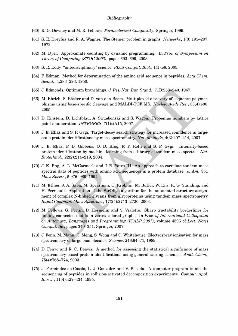
DRAFT

Bibliography

[60] R. G. Downey and M. R. Fellows. Parameterized Complexity. Springer, 1999.

[61] S. E. Dreyfus and R. A. Wagner. The Steiner problem in graphs. Networks, 1(3):195–207,1972.

[62] M. Dyer. Approximate counting by dynamic programming. In Proc. of Symposium onTheory of Computing (STOC 2003), pages 693–699, 2003.

[63] S. R. Eddy. “antedisciplinary” science. PLoS Comput. Biol., 1(1):e6, 2005.

[64] P. Edman. Method for determination of the amino acid sequence in peptides. Acta Chem.Scand., 4:283–293, 1950.

[65] J. Edmonds. Optimum branchings. J. Res. Nat. Bur. Stand., 71B:233–240, 1967.

[66] M. Ehrich, S. Böcker and D. van den Boom. Multiplexed discovery of sequence polymor-phisms using base-specific cleavage and MALDI-TOF MS. Nucleic Acids Res., 33(4):e38,2005.

[67] D. Einstein, D. Lichtblau, A. Strzebonski and S. Wagon. Frobenius numbers by latticepoint enumeration. INTEGERS, 7(1):#A15, 2007.

[68] J. E. Elias and S. P. Gygi. Target-decoy search strategy for increased confidence in large-scale protein identifications by mass spectrometry. Nat. Methods, 4(3):207–214, 2007.

[69] J. E. Elias, F. D. Gibbons, O. D. King, F. P. Roth and S. P. Gygi. Intensity-basedprotein identification by machine learning from a library of tandem mass spectra. Nat.Biotechnol., 22(2):214–219, 2004.

[70] J. K. Eng, A. L. McCormack and J. R. Yates III. An approach to correlate tandem massspectral data of peptides with amino acid sequences in a protein database. J. Am. Soc.Mass Spectr., 5:976–989, 1994.

[71] M. Ethier, J. A. Saba, M. Spearman, O. Krokhin, M. Butler, W. Ens, K. G. Standing, andH. Perreault. Application of the StrOligo algorithm for the automated structure assign-ment of complex N-linked glycans from glycoproteins using tandem mass spectrometry.Rapid Commun. Mass Spectrom., 17(24):2713–2720, 2003.

[72] M. Fellows, G. Fertin, D. Hermelin and S. Vialette. Sharp tractability borderlines forfinding connected motifs in vertex-colored graphs. In Proc. of International Colloquiumon Automata, Languages and Programming (ICALP 2007), volume 4596 of Lect. NotesComput. Sc., pages 340–351. Springer, 2007.

[73] J. Fenn, M. Mann, C. Meng, S. Wong and C. Whitehouse. Electrospray ionisation for massspectrometry of large biomolecules. Science, 246:64–71, 1989.

[74] D. Fenyö and R. C. Beavis. A method for assessing the statistical significance of massspectrometry-based protein identifications using general scoring schemes. Anal. Chem.,75(4):768–774, 2003.

[75] J. Fernández-de-Cossío, L. J. Gonzalez and V. Besada. A computer program to aid thesequencing of peptides in collision-activated decomposition experiments. Comput. Appl.Biosci., 11(4):427–434, 1995.

181

DRAFT

Bibliography

[76] J. Fernández-de-Cossío, J. Gonzalez, T. Takao, Y. Shimonishi, G. Padron and V. Besada.A software program for the rapid sequence analysis of unknown peptides involvingmodifications, based on MS/MS data. In ASMS Conf. on Mass Spectrometry and AlliedTopics, Slot 074, 1997.

[77] J. Fernández-de-Cossío, L. J. Gonzalez, Y. Satomi, L. Betancourt, Y. Ramos, V. Huerta,A. Amaro, V. Besada, G. Padron, N. Minamino, and T. Takao. Isotopica: a tool for thecalculation and viewing of complex isotopic envelopes. Nucleic Acids Res., 32(Web Serverissue):W674–W678, 2004.

[78] A. R. Fernie, R. N. Trethewey, A. J. Krotzky and L. Willmitzer. Metabolite profiling: fromdiagnostics to systems biology. Nat. Rev. Mol. Cell Biol., 5(9):763–769, 2004.

[79] H. I. Field, D. Fenyö and R. C. Beavis. RADARS, a bioinformatics solution that automatesproteome mass spectral analysis, optimises protein identification, and archives data in arelational database. Proteomics, 2(1):36–47, 2002.

[80] B. Fischer, V. Roth, F. Roos, J. Grossmann, S. Baginsky, P. Widmayer, W. Gruissem, andJ. M. Buhmann. NovoHMM: a hidden Markov model for de novo peptide sequencing. Anal.Chem., 77(22):7265–7273, 2005.

[81] P. Flajolet and R. Sedgewick. Analytic Combinatorics. Cambridge University Press, 2009.Freely available from http://algo.inria.fr/flajolet/Publications/book.pdf.

[82] A. Frank and P. Pevzner. PepNovo: de novo peptide sequencing via probabilistic networkmodeling. Anal. Chem., 15:964–973, 2005.

[83] A. M. Frank, M. M. Savitski, M. N. Nielsen, R. A. Zubarev and P. A. Pevzner. De novopeptide sequencing and identification with precision mass spectrometry. J. Proteome Res.,6(1):114–123, 2007.

[84] A. Fürst, J.-T. Clerc and E. Pretsch. A computer program for the computation of themolecular formula. Chemom. Intell. Lab. Syst., 5:329–334, 1989.

[85] V. A. Fusaro, D. R. Mani, J. P. Mesirov and S. A. Carr. Prediction of high-respondingpeptides for targeted protein assays by mass spectrometry. Nat. Biotechnol., 27(2):190–198, 2009.

[86] H. Gabow, Z. Galil, T. Spencer and R. Tarjan. Efficient algorithms for finding minimumspanning trees in undirected and directed graphs. Combinatorica, 6:109–122, 1986.

[87] M. R. Garey and D. S. Johnson. Computers and Intractability (A Guide to Theory of NP-Completeness). Freeman, New York, 1979.

[88] J. Gasteiger, W. Hanebeck and K.-P. Schulz. Prediction of mass spectra from structuralinformation. J. Chem. Inf. Comput. Sci., 32(4):264–271, 1992.

[89] S. P. Gaucher, J. Morrow and J. A. Leary. STAT: a saccharide topology analysis tool usedin combination with tandem mass spectrometry. Anal. Chem., 72(11):2331–2336, 2000.

[90] L. Y. Geer, S. P. Markey, J. A. Kowalak, L. Wagner, M. Xu, D. M. Maynard, X. Yang, W. Shi,and S. H. Bryant. Open mass spectrometry search algorithm. J. Proteome Res., 3:958–964,2004.

182

DRAFT

Bibliography

[91] P. Gilmore and R. Gomory. Multi-stage cutting stock problems of two and more dimen-sions. Oper. Res., 13(1):94–120, 1965.

[92] D. Goldberg, M. Sutton-Smith, J. Paulson and A. Dell. Automatic annotation of matrix-assisted laser desorption/ionization N-glycan spectra. Proteomics, 5(4):865–875, 2005.

[93] D. Goldberg, M. W. Bern, B. Li and C. B. Lebrilla. Automatic determination of O-glycanstructure from fragmentation spectra. J. Proteome Res., 5(6):1429–1434, 2006.

[94] D. Goldberg, M. W. Bern, S. Parry, M. Sutton-Smith, M. Panico, H. R. Morris and A. Dell.Automated N-glycopeptide identification using a combination of single- and tandem-MS.J. Proteome Res., 6(10):3995–4005, 2007.

[95] D. Goldberg, M. W. Bern, S. J. North, S. M. Haslam and A. Dell. Glycan family analysisfor deducing N-glycan topology from single MS. Bioinformatics, 25(3):365–371, 2009.

[96] A. H. Grange, M. C. Zumwalt and G. W. Sovocool. Determination of ion and neutralloss compositions and deconvolution of product ion mass spectra using an orthogonalacceleration time-of-flight mass spectrometer and an ion correlation program. RapidCommun. Mass Spectrom., 20(2):89–102, 2006.

[97] N. A. Gray. Applications of artificial intelligence for organic chemistry: Analysis of C-13spectra. Artificial Intelligence, 22(1):1–21, 1984.

[98] N. A. B. Gray, R. E. Carhart, A. Lavanchy, D. H. Smith, T. Varkony, B. G. Buchanan, W. C.White, and L. Creary. Computerized mass spectrum prediction and ranking. Anal. Chem.,52(7):1095–1102, 1980.

[99] N. A. B. Gray, A. Buchs, D. H. Smith and C. Djerassi. Computer assisted structuralinterpretation of mass spectral data. Helv. Chim. Acta, 64(2):458–470, 1981.

[100] H. Greenberg. Solution to a linear diophantine equation for nonnegative integers. J.Algorithms, 9(3):343–353, 1988.

[101] D. H. Greene and D. E. Knuth. Mathematics for the Analysis of Algorithms, volume 1 ofProgress in Computer Science and Applied Logic (PCS). Birkhäuser Boston, 1990.

[102] J. Gross. Mass Spectrometry: A textbook. Springer, Berlin, 2004.

[103] K. Grützmann, S. Böcker and S. Schuster. Combinatorics of aliphatic amino acids.Naturwissenschaften, 98(1):79–86, 2011.

[104] M. Guilhaus. Principles and instrumentation in time-of-flight mass spectrometry. J. MassSpectrom., 30:1519–1532, 1995.

[105] S. Guillemot and F. Sikora. Finding and counting vertex-colored subtrees. In Proc. ofSymposium on Mathematical Foundations of Computer Science (MFCS 2010), volume6281 of Lect. Notes Comput. Sc., pages 405–416. Springer, 2010.

[106] C. Hamm, W. Wilson and D. Harvan. Peptide sequencing program. Comput. Appl. Biosci.,2:115–118, 1986.

183

DRAFT

Bibliography

[107] F. Harary, R. W. Robinson and A. J. Schwenk. Twenty-step algorithm for determiningthe asymptotic number of trees of various species. J. Austral. Math. Soc., 20(Series A):483–503, 1975.

[108] M. Havilio, Y. Haddad and Z. Smilansky. Intensity-based statistical scorer for tandemmass spectrometry. Anal. Chem., 75:435–444, 2003.

[109] M. Heinonen, A. Rantanen, T. Mielikäinen, J. Kokkonen, J. Kiuru, R. A. Ketola andJ. Rousu. FiD: a software for ab initio structural identification of product ions from tandemmass spectrometric data. Rapid Commun. Mass Spectrom., 22(19):3043–3052, 2008.

[110] D. W. Hill, T. M. Kertesz, D. Fontaine, R. Friedman and D. F. Grant. Mass spectralmetabonomics beyond elemental formula: Chemical database querying by matchingexperimental with computational fragmentation spectra. Anal. Chem., 80(14):5574–5582,2008.

[111] W. M. Hines, A. M. Falick, A. L. Burlingame and B. W. Gibson. Pattern-based algorithm forpeptide sequencing from tandem high energy collision-induced dissociation mass spectra.J. Am. Soc. Mass Spectrom., 3(4):326 – 336, 1992.

[112] C. A. R. Hoare. FIND (algorithm 65). Communications of the ACM, 4:321–322, 1961.

[113] D. H. Horn, R. A. Zubarev and F. W. McLafferty. Automated reduction and interpretationof high resolution electrospray mass spectra of large molecules. J. Am. Soc. Mass Spectr.,11:320–332, 2000.

[114] C. S. Hsu. Diophantine approach to isotopic abundance calculations. Anal. Chem., 56(8):1356–1361, 1984.

[115] Q. Hu, R. J. Noll, H. Li, A. Makarov, M. Hardman and R. G. Cooks. The Orbitrap: a newmass spectrometer. J. Mass Spectrom., 40(4):430–443, 2005.

[116] R. Hussong and A. Hildebrandt. Signal processing in proteomics. Methods Mol. Biol., 604:145–161, 2010.

[117] N. Jaitly, M. E. Monroe, V. A. Petyuk, T. R. W. Clauss, J. N. Adkins and R. D. Smith.Robust algorithm for alignment of liquid chromatography-mass spectrometry analyses inan accurate mass and time tag data analysis pipeline. Anal. Chem., 78(21):7397–7409,2006.

[118] N. Jeffries. Algorithms for alignment of mass spectrometry proteomic data. Bioinformat-ics, 21(14):3066–3073, 2005.

[119] R. S. Johnson and J. A. Taylor. Searching sequence databases via de novo peptidesequencing by tandem mass spectrometry. Methods Mol. Biol., 146:41–61, 2000.

[120] R. S. Johnson and J. A. Taylor. Searching sequence databases via de novo peptidesequencing by tandem mass spectrometry. Mol. Biotechnol., 22(3):301–315, 2002.

[121] P. Jones, R. G. Côté, L. Martens, A. F. Quinn, C. F. Taylor, W. Derache, H. Hermjakob,and R. Apweiler. PRIDE: a public repository of protein and peptide identifications for theproteomics community. Nucleic Acids Res., 34(Database-Issue):659–663, 2006.

184

DRAFT

Bibliography

[122] H. J. Joshi, M. J. Harrison, B. L. Schulz, C. A. Cooper, N. H. Packer and N. G. Karlsson.Development of a mass fingerprinting tool for automated interpretation of oligosaccharidefragmentation data. Proteomics, 4(6):1650–1664, 2004.

[123] L. Käll, J. D. Canterbury, J. Weston, W. S. Noble and M. J. MacCoss. Semi-supervisedlearning for peptide identification from shotgun proteomics datasets. Nat. Methods, 4(11):923–925, 2007.

[124] M. Kanehisa, S. Goto, M. Hattori, K. F. Aoki-Kinoshita, M. Itoh, S. Kawashima,T. Katayama, M. Araki, and M. Hirakawa. From genomics to chemical genomics: newdevelopments in KEGG. Nucleic Acids Res., 34:D354–D357, 2006.

[125] R. Kannan. Lattice translates of a polytope and the Frobenius problem. Combinatorica,12:161–177, 1991.

[126] E. A. Kapp, F. Schütz, L. M. Connolly, J. A. Chakel, J. E. Meza, C. A. Miller, D. Fenyo, J. K.Eng, J. N. Adkins, G. S. Omenn, and R. J. Simpson. An evaluation, comparison, and ac-curate benchmarking of several publicly available MS/MS search algorithms: Sensitivityand specificity analysis. Proteomics, 5:3475–3490, 2005.

[127] M. Karas and F. Hillenkamp. Laser desorption ionization of proteins with molecularmasses exceeding 10,000 Daltons. Anal. Chem., 60:2299–2301, 1988.

[128] A. Keller, A. I. Nesvizhskii, E. Kolker and R. Aebersold. Empirical statistical model toestimate the accuracy of peptide identifications made by MS/MS and database search.Anal. Chem., 74(20):5383–5392, 2002.

[129] A. Keller, J. Eng, N. Zhang, X.-J. Li and R. Aebersold. A uniform proteomics MS/MSanalysis platform utilizing open XML file formats. Mol. Syst. Biol., 1:2005.0017, 2005.

[130] E. Kendrick. A mass scale based on CH2 = 14.0000 for high resolution mass spectrometryof organic compounds. Anal. Chem., 35(13):2146–2154, 1963.

[131] A. Kerber, R. Laue and D. Moser. Ein Strukturgenerator für molekulare Graphen. Anal.Chim. Acta, 235:221 – 228, 1990.

[132] A. Kerber, R. Laue, M. Meringer and C. Rücker. Molecules in silico: The generation ofstructural formulae and its applications. J. Comput. Chem. Japan, 3(3):85–96, 2004.

[133] S. Kim, N. Gupta and P. A. Pevzner. Spectral probabilities and generating functions oftandem mass spectra: a strike against decoy databases. J. Proteome Res., 7(8):3354–3363,2008.

[134] S. Kim, N. Bandeira and P. A. Pevzner. Spectral profiles, a novel representation of tandemmass spectra and their applications for de novo peptide sequencing and identification.Mol. Cell. Proteomics, 8(6):1391–1400, 2009.

[135] S. Kim, N. Gupta, N. Bandeira and P. A. Pevzner. Spectral dictionaries: Integratingde novo peptide sequencing with database search of tandem mass spectra. Mol. Cell.Proteomics, 8(1):53–69, 2009.

185

DRAFT

Bibliography

[136] T. Kind and O. Fiehn. Metabolomic database annotations via query of elemental compo-sitions: Mass accuracy is insufficient even at less than 1 ppm. BMC Bioinformatics, 7(1):234, 2006.

[137] T. Kind and O. Fiehn. Seven golden rules for heuristic filtering of molecular formulasobtained by accurate mass spectrometry. BMC Bioinformatics, 8:105, 2007.

[138] H. Kubinyi. Calculation of isotope distributions in mass spectrometry: A trivial solutionfor a non-trivial problem. Anal. Chim. Acta, 247:107–119, 1991.

[139] K.-S. Kwok, R. Venkataraghavan and F. W. McLafferty. Computer-aided interpretation ofmass spectra. III. Self-training interpretive and retrieval system. J. Am. Chem. Soc., 95(13):4185–4194, 1973.

[140] V. Lacroix, C. G. Fernandes, and M.-F. Sagot. Motif search in graphs: Application tometabolic networks. IEEE/ACM Trans. Comput. Biol. Bioinform., 3(4):360–368, 2006.

[141] A. J. Lapadula, P. J. Hatcher, A. J. Hanneman, D. J. Ashline, H. Zhang and V. N. Reinhold.Congruent strategies for carbohydrate sequencing. 3. OSCAR: an algorithm for assigningoligosaccharide topology from MSn data. Anal. Chem., 77(19):6271–6279, 2005.

[142] R. L. Last, A. D. Jones and Y. Shachar-Hill. Towards the plant metabolome and beyond.Nat. Rev. Mol. Cell Biol., 8:167–174, 2007.

[143] A. Lavanchy, T. Varkony, D. H. Smith, N. A. B. Gray, W. C. White, R. E. Carhart,B. G. Buchanan, and C. Djerassi. Rule-based mass spectrum prediction and ranking:Applications to structure elucidation of novel marine sterols. Org. Mass Spectrom., 15(7):355–366, 1980.

[144] J. Lederberg. Topological mapping of organic molecules. Proc. Natl. Acad. Sci. U. S. A., 53(1):134–139, 1965.

[145] J. Lederberg. How DENDRAL was conceived and born. In ACM Conference on theHistory of Medical Informatics, History of Medical Informatics archive, pages 5–19, 1987.Available from http://doi.acm.org/10.1145/41526.41528.

[146] T. A. Lee. A Beginner’s Guide to Mass Spectral Interpretation. Wiley, 1998.

[147] M. Lefmann, C. Honisch, S. Boecker, N. Storm, F. von Wintzingerode, C. Schloetelburg,A. Moter, D. van den Boom, and U. B. Goebel. A novel mass spectrometry based tool forgenotypic identification of mycobacteria. J. Clin. Microbiol., 42(1):339–346, 2004.

[148] G. Li and F. Ruskey. The advantages of forward thinking in generating rooted and freetrees. In Proc. of ACM-SIAM Symposium on Discrete Algorithms (SODA 1999), pages939–940, Philadelphia, PA, USA, 1999. Society for Industrial and Applied Mathematics.

[149] G. Liu, J. Zhang, B. Larsen, C. Stark, A. Breitkreutz, Z.-Y. Lin, B.-J. Breitkreutz, Y. Ding,K. Colwill, A. Pasculescu, T. Pawson, J. L. Wrana, A. I. Nesvizhskii, B. Raught, M. Tyers,and A.-C. Gingras. ProHits: integrated software for mass spectrometry-based interactionproteomics. Nat. Biotechnol., 28(10):1015–1017, 2010.

186

DRAFT

Bibliography

[150] K. K. Lohmann and C.-W. von der Lieth. GlycoFragment and GlycoSearchMS: web tools tosupport the interpretation of mass spectra of complex carbohydrates. Nucleic Acids Res.,32(Web Server issue):W261–W266, 2004.

[151] B. Lu and T. Chen. A suffix tree approach to the interpretation of tandem mass spectra:Applications to peptides of non-specific digestion and post-translational modifications.Bioinformatics, 19(Suppl 2):ii113–ii121, 2003. Proc. of European Conference on Computa-tional Biology (ECCB 2003).

[152] A. Luedemann, K. Strassburg, A. Erban and J. Kopka. TagFinder for the quantitativeanalysis of gas chromatography–mass spectrometry (GC-MS)-based metabolite profilingexperiments. Bioinformatics, 24(5):732–737, 2008.

[153] G. S. Lueker. Two NP-complete problems in nonnegative integer programming. TechnicalReport TR-178, Department of Electrical Engineering, Princeton University, 1975.

[154] Y.-R. Luo. Handbook of Bond Dissociation Energies in Organic Compounds. CRC Press,Boca Raton, 2003.

[155] B. Ma and G. Lajoie. Improving the de novo sequencing accuracy by combining twoindependent scoring functions in peaks software. Poster at the ASMS Conference on MassSpectrometry and Allied Topics, 2005.

[156] B. Ma, K. Zhang, C. Hendrie, C. Liang, M. Li, A. Doherty-Kirby and G. Lajoie. PEAKS:powerful software for peptide de novo sequencing by tandem mass spectrometry. RapidCommun. Mass Spectrom., 17(20):2337–2342, 2003.

[157] B. Ma, K. Zhang and C. Liang. An effective algorithm for peptide de novo sequencing fromMS/MS spectra. J. Comput. Syst. Sci., 70:418–430, 2005.

[158] K. Maass, R. Ranzinger, H. Geyer, C.-W. von der Lieth and R. Geyer. “Glyco-peakfinder” –de novo composition analysis of glycoconjugates. Proteomics, 7(24):4435–4444, 2007.

[159] P. Mallick, M. Schirle, S. S. Chen, M. R. Flory, H. Lee, D. Martin, J. Ranish, B. Raught,R. Schmitt, T. Werner, B. Kuster, and R. Aebersold. Computational prediction of proteo-typic peptides for quantitative proteomics. Nat. Biotechnol., 25(1):125–131, 2007.

[160] M. Mann and M. Wilm. Error-tolerant identification of peptides in sequence databases bypeptide sequence tags. Anal. Chem., 66(24):4390–4399, 1994.

[161] S. Martello and P. Toth. An exact algorithm for large unbounded knapsack problems.Oper. Res. Lett., 9(1):15–20, 1990.

[162] S. Martello and P. Toth. Knapsack Problems: Algorithms and Computer Implementations.John Wiley & Sons, Chichester, 1990.

[163] R. Matthiesen, J. Bunkenborg, A. Stensballe, O. N. Jensen, K. G. Welinder and G. Bauw.Database-independent, database-dependent, and extended interpretation of peptide massspectra in VEMS V2.0. Proteomics, 4(9):2583–2593, 2004.

[164] R. Matthiesen, M. B. Trelle, P. Hojrup, J. Bunkenborg and O. N. Jensen. VEMS 3.0:algorithms and computational tools for tandem mass spectrometry based identification ofpost-translational modifications in proteins. J. Proteome Res., 4(6):2338–2347, 2005.

187

DRAFT

Bibliography

[165] L. McHugh and J. W. Arthur. Computational methods for protein identification from massspectrometry data. PLoS Comput. Biol., 4(2):e12, 2008.

[166] P. E. Miller and M. B. Denton. The quadrupole mass filter: Basic operating concepts. J.Chem. Educ., 63:617–622, 1986.

[167] L. Mo, D. Dutta, Y. Wan and T. Chen. MSNovo: a dynamic programming algorithm for denovo peptide sequencing via tandem mass spectrometry. Anal. Chem., 79(13):4870–4878,2007.

[168] E. Mostacci, C. Truntzer, H. Cardot and P. Ducoroy. Multivariate denoising methodscombining wavelets and principal component analysis for mass spectrometry data. Pro-teomics, 10(14):2564–2572, 2010.

[169] I. K. Mun and F. W. Mclafferty. Computer methods of molecular structure elucidationfrom unknown mass spectra. In Supercomputers in Chemistry, ACS Symposium Series,chapter 9, pages 117–124. American Chemical Society, 1981.

[170] S. Na, J. Jeong, H. Park, K.-J. Lee and E. Paek. Unrestrictive identification of multiplepost-translational modifications from tandem mass spectrometry using an error-tolerantalgorithm based on an extended sequence tag approach. Mol. Cell. Proteomics, 7(12):2452–2463, 2008.

[171] S. Neumann and S. Böcker. Computational mass spectrometry for metabolomics – areview. Anal. Bioanal. Chem., 398(7):2779–2788, 2010.

[172] N. Nguyen, H. Huang, S. Oraintara and A. Vo. Mass spectrometry data processing usingzero-crossing lines in multi-scale of Gaussian derivative wavelet. Bioinformatics, 26(18):i659–i665, 2010.

[173] R. Niedermeier. Invitation to Fixed-Parameter Algorithms. Oxford University Press, 2006.

[174] J. A. November. Digitizing life: the introduction of computers to biology and medicine.PhD thesis, Princeton University, Princeton, USA, 2006.

[175] H. Oberacher, M. Pavlic, K. Libiseller, B. Schubert, M. Sulyok, R. Schuhmacher,E. Csaszar, and H. C. Köfeler. On the inter-instrument and inter-laboratory transferabilityof a tandem mass spectral reference library: 1. results of an austrian multicenter study.J. Mass Spectrom., 44(4):485–493, 2009.

[176] H. Oberacher, M. Pavlic, K. Libiseller, B. Schubert, M. Sulyok, R. Schuhmacher,E. Csaszar, and H. C. Köfeler. On the inter-instrument and the inter-laboratory transfer-ability of a tandem mass spectral reference library: 2. optimization and characterizationof the search algorithm. J. Mass Spectrom., 44(4):494–502, 2009.

[177] S. Orchard, L. Montechi-Palazzi, E. W. Deutsch, P.-A. Binz, A. R. Jones, N. Paton,A. Pizarro, D. M. Creasy, J. Wojcik, and H. Hermjakob. Five years of progress in thestandardization of proteomics data: 4th annual spring workshop of the HUPO-proteomicsstandards initiative. Proteomics, 7:3436–3440, 2007.

[178] R. Otter. The number of trees. The Annals of Mathematics, 49(3):583–599, 1948.

188

DRAFT

Bibliography

[179] K. G. Owens. Application of correlation analysis techniques to mass spectral data. Appl.Spectrosc. Rev., 27(1):1–49, 1992.

[180] N. H. Packer, C.-W. von der Lieth, K. F. Aoki-Kinoshita, C. B. Lebrilla, J. C. Paulson,R. Raman, P. Rudd, R. Sasisekharan, N. Taniguchi, and W. S. York. Frontiers in glycomics:bioinformatics and biomarkers in disease. An NIH white paper prepared from discussionsby the focus groups at a workshop on the NIH campus, Bethesda MD (September 11-13,2006). Proteomics, 8(1):8–20, 2008.

[181] G. Palmisano, D. Antonacci and M. R. Larsen. Glycoproteomic profile in wine: a ‘sweet’molecular renaissance. J. Proteome Res., 9(12):6148–6159, 2010.

[182] D. J. Pappin, P. Hojrup and A. Bleasby. Rapid identification of proteins by peptide-massfingerprinting. Curr. Biol., 3(6):327–332, 1993.

[183] C. Y. Park, A. A. Klammer, L. Käll, M. J. MacCoss and W. S. Noble. Rapid and accuratepeptide identification from tandem mass spectra. J. Proteome Res., 7(7):3022–3027, 2008.

[184] W. E. Parkins. The uranium bomb, the calutron, and the space-charge problem. PhysicsToday, 58(5):45–51, 2005.

[185] V. Pellegrin. Molecular formulas of organic compounds: the nitrogen rule and degree ofunsaturation. J. Chem. Educ., 60(8):626–633, 1983.

[186] D. N. Perkins, D. J. Pappin, D. M. Creasy and J. S. Cottrell. Probability-based protein iden-tification by searching sequence databases using mass spectrometry data. Electrophoresis,20(18):3551–3567, 1999.

[187] R. H. Perry, R. G. Cooks and R. J. Noll. Orbitrap mass spectrometry: instrumentation, ionmotion and applications. Mass Spectrom. Rev., 27(6):661–699, 2008.

[188] G. Pólya. Kombinatorische Anzahlbestimmungen für Gruppen, Graphen und chemischeVerbindungen. Acta Mathematica, 68(1):145–254, 1937.

[189] S. C. Pomerantz, J. A. Kowalak and J. A. McCloskey. Determination of oligonucleotidecomposition from mass spectromectrically measured molecular weight. J. Am. Soc. MassSpectrom., 4:204–209, 1993.

[190] R. Raman, S. Raguram, G. Venkataraman, J. C. Paulson and R. Sasisekharan. Glycomics:an integrated systems approach to structure-function relationships of glycans. Nat.Methods, 2(11):817–824, 2005.

[191] J. L. Ramírez-Alfonsín. The Diophantine Frobenius Problem. Oxford University Press,2005.

[192] J. L. Ramírez-Alfonsín. Complexity of the Frobenius problem. Combinatorica, 16(1):143–147, 1996.

[193] I. Rauf, F. Rasche and S. Böcker. Computing maximum colorful subtrees in practice.Manuscript. [TODO: REMOVE OR UPDATE], 2011.

[194] A. L. Rockwood and P. Haimi. Efficient calculation of accurate masses of isotopic peaks.J. Am. Soc. Mass Spectrom., 17(3):415–419, 2006.

189

DRAFT

Bibliography

[195] A. L. Rockwood, M. M. Kushnir and G. J. Nelson. Dissociation of individual isotopic peaks:Predicting isotopic distributions of product ions in MSn. J. Am. Soc. Mass Spectr., 14:311–322, 2003.

[196] A. L. Rockwood, J. R. Van Orman and D. V. Dearden. Isotopic compositions and accuratemasses of single isotopic peaks. J. Am. Soc. Mass Spectr., 15:12–21, 2004.

[197] P. Roepstorff and J. Fohlman. Proposal for a common nomenclature for sequence ions inmass spectra of peptides. Biomed. Mass Spectrom., 11(11):601, 1984.

[198] S. Rogers, R. A. Scheltema, M. Girolami and R. Breitling. Probabilistic assignment offormulas to mass peaks in metabolomics experiments. Bioinformatics, 25(4):512–518,2009.

[199] R. G. Sadygov and J. R. Yates III. A hypergeometric probability model for proteinidentification and validation using tandem mass spectral data and protein sequencedatabases. Anal. Chem., 75(15):3792–3798, 2003.

[200] R. G. Sadygov, D. Cociorva and J. R. Yates III. Large-scale database searching usingtandem mass spectra: looking up the answer in the back of the book. Nat. Methods, 1(3):195–202, 2004.

[201] T. Sakurai, T. Matsuo, H. Matsuda and I. Katakuse. PAAS 3: A computer program todetermine probable sequence of peptides from mass spectrometric data. Biomed. MassSpectrom., 11(8):396–399, 1984.

[202] A. Salomaa. Counting (scattered) subwords. B. Euro. Assoc. Theo. Comp. Sci., 81:165–179,2003.

[203] F. Sanger, S. Nicklen and A. R. Coulson. DNA sequencing with chain-terminatinginhibitors. Proc. Natl. Acad. Sci. U.S.A., 74(12):5463–5467, 1977.

[204] M. M. Savitski, M. L. Nielsen, F. Kjeldsen and R. A. Zubarev. Proteomics-grade de novosequencing approach. J. Proteome Res., 4:2348–2354, 2005.

[205] K. Scheubert, F. Hufsky, F. Rasche and S. Böcker. Computing fragmentation trees frommetabolite multiple mass spectrometry data. In Proc. of Research in ComputationalMolecular Biology (RECOMB 2011), volume 6577 of Lect. Notes Comput. Sc., pages 377–391. Springer, 2011.

[206] J. Seidler, N. Zinn, M. E. Boehm and W. D. Lehmann. De novo sequencing of peptides byMS/MS. Proteomics, 10(4):634–649, 2010.

[207] J. Senior. Partitions and their representative graphs. Am. J. Math., 73(3):663–689, 1951.

[208] B. Shan, B. Ma, K. Zhang and G. Lajoie. Complexities and algorithms for glycan sequenc-ing using tandem mass spectrometry. J. Bioinformatics and Computational Biology, 6(1):77–91, 2008.

[209] Q. Sheng, Y. Mechref, Y. Li, M. V. Novotny and H. Tang. A computational ap-proach to characterizing bond linkages of glycan isomers using matrix-assisted laserdesorption/ionization tandem time-of-flight mass spectrometry. Rapid Commun. MassSpectrom., 22(22):3561–3569, 2008.

190

DRAFT

Bibliography

[210] I. V. Shilov, S. L. Seymour, A. A. Patel, A. Loboda, W. H. Tang, S. P. Keating, C. L.Hunter, L. M. Nuwaysir, and D. A. Schaeffer. The paragon algorithm, a next generationsearch engine that uses sequence temperature values and feature probabilities to identifypeptides from tandem mass spectra. Mol. Cell. Proteomics, 6(9):1638–1655, 2007.

[211] H. Shin, M. P. Sampat, J. M. Koomen and M. K. Markey. Wavelet-based adaptive denoisingand baseline correction for MALDI TOF MS. OMICS, 14(3):283–295, 2010.

[212] F. Sikora. An (almost complete) state of the art around the graph motif problem. Technicalreport, Université Paris-Est, France, 2010. Available from http://www-igm.univ-mlv.

fr/~fsikora/pub/GraphMotif-Resume.pdf.

[213] R. M. Silverstein, F. X. Webster and D. Kiemle. Spectrometric Identification of OrganicCompounds. Wiley, 7th edition, 2005.

[214] G. Siuzdak. The Expanding Role of Mass Spectrometry in Biotechnology. MCC Press,second edition, 2006.

[215] D. H. Smith, N. A. Gray, J. G. Nourse and C. W. Crandell. The DENDRAL project: recentadvances in computer-assisted structure elucidation. Anal. Chim. Acta, 133(4):471 – 497,1981.

[216] R. K. Snider. Efficient calculation of exact mass isotopic distributions. J. Am. Soc. MassSpectrom., 18(8):1511–1515, 2007.

[217] H. M. Sobell. Actinomycin and DNA transcription. Proc. Natl. Acad. Sci. U. S. A., 82(16):5328–5331, 1985.

[218] H. Steen and M. Mann. The ABC’s (and XYZ’s) of peptide sequencing. Nature Rev., 5:699–711, 2004.

[219] M. T. Sykes and J. R. Williamson. Envelope: interactive software for modeling and fittingcomplex isotope distributions. BMC Bioinformatics, 9:446, 2008.

[220] J. J. Sylvester and W. J. Curran Sharp. Problem 7382. Educational Times, 37:26, 1884.

[221] D. L. Tabb, M. J. MacCoss, C. C. Wu, S. D. Anderson and J. R. Yates. Similarity amongtandem mass spectra from proteomic experiments: detection, significance, and utility.Anal. Chem., 75(10):2470–2477, 2003.

[222] H. Tang, Y. Mechref and M. V. Novotny. Automated interpretation of MS/MS spectra ofoligosaccharides. Bioinformatics, 21 Suppl 1:i431–i439, 2005. Proc. of Intelligent Systemsfor Molecular Biology (ISMB 2005).

[223] S. Tanner, H. Shu, A. Frank, L.-C. Wang, E. Zandi, M. Mumby, P. A. Pevzner, and V. Bafna.Inspect: Identification of posttranslationally modified peptides from tandem mass spectra.Anal. Chem., 77:4626–4639, 2005.

[224] J. A. Taylor and R. S. Johnson. Implementation and uses of automated de novo peptidesequencing by tandem mass spectrometry. Anal. Chem., 73(11):2594–2604, 2001.

[225] J. A. Taylor and R. S. Johnson. Sequence database searches via de novo peptide sequencingby tandem mass spectrometry. Rapid Commun. Mass Spectrom., 11:1067–1075, 1997.

191

DRAFT

Bibliography

[226] J. van Lint and R. Wilson. A Course in Combinatorics. Cambridge University Press, 2001.

[227] A. Varki, R. D. Cummings, J. D. Esko, H. H. Freeze, P. Stanley, C. R. Bertozzi, G. W. Hart,and M. E. Etzler, editors. Essentials of Glycobiology. Cold Spring Harbor LaboratoryPress, second edition, 2009. Freely available from http://www.ncbi.nlm.nih.gov/

books/NBK1908/.

[228] R. Venkataraghavan, F. W. McLafferty and G. E. van Lear. Computer-aided interpretationof mass spectra. Org. Mass Spectrom., 2(1):1–15, 1969.

[229] C.-W. von der Lieth, A. Bohne-Lang, K. K. Lohmann and M. Frank. Bioinformatics forglycomics: status, methods, requirements and perspectives. Brief. Bioinform., 5(2):164–178, 2004.

[230] S. A. Waksman and H. B. Woodruff. Bacteriostatic and bacteriocidal substances producedby soil actinomycetes. Proc. Soc. Exper. Biol., 45:609–614, 1940.

[231] M. S. Waterman and M. Vingron. Rapid and accurate estimates of statistical significancefor sequence data base searches. Proc. Natl. Acad. Sci. U. S. A., 91(11):4625–4628, 1994.

[232] J. T. Watson and O. D. Sparkman. Introduction to Mass Spectrometry: Instrumentation,Applications, and Strategies for Data Interpretation. Wiley, 2007.

[233] M. E. Wieser. Atomic weights of the elements 2005 (IUPAC technical report). Pure Appl.Chem., 78(11):2051–2066, 2006.

[234] H. Wilf. generatingfunctionology. Academic Press, second edition, 1994. Freely availablefrom http://www.math.upenn.edu/~wilf/DownldGF.html.

[235] S. Wolf, S. Schmidt, M. Müller-Hannemann and S. Neumann. In silico fragmentation forcomputer assisted identification of metabolite mass spectra. BMC Bioinformatics, 11:148,2010.

[236] W. E. Wolski, M. Lalowski, P. Jungblut and K. Reinert. Calibration of mass spectrometricpeptide mass fingerprint data without specific external or internal calibrants. BMCBioinformatics, 6:203, 2005.

[237] J. W. Wong, G. Cagney and H. M. Cartwright. SpecAlign—processing and alignment ofmass spectra datasets. Bioinformatics, 21(9):2088–2090, 2005.

[238] L.-C. Wu, H.-H. Chen, J.-T. Horng, C. Lin, N. E. Huang, Y.-C. Cheng and K.-F. Cheng. Anovel preprocessing method using Hilbert Huang transform for MALDI-TOF and SELDI-TOF mass spectrometry data. PLoS One, 5(8):e12493, 2010.

[239] Y. Wu, Y. Mechref, I. Klouckova, M. V. Novotny and H. Tang. A computational approach forthe identification of site-specific protein glycosylations through ion-trap mass spectrome-try. In Proc. of RECOMB 2006 satellite workshop on Systems biology and computationalproteomics, volume 4532 of Lect. Notes Comput. Sc., pages 96–107. Springer, 2007.

[240] C. Xu and B. Ma. Complexity and scoring function of MS/MS peptide de novo sequencing.In Proc. of Computational Systems Bioinformatics Conference (CSB 2006), volume 4of Series on Advances in Bioinformatics and Computational Biology, pages 361–369.Imperial College Press, 2006.

192

DRAFT

Bibliography

[241] J. Yates, P. Griffin, L. Hood and J. Zhou. Computer aided interpretation of low energyMS/MS mass spectra of peptides. In J. Villafranca, editor, Techniques in Protein ChemistryII, pages 477–485. Academic Press, San Diego, 1991.

[242] J. A. Yergey. A general approach to calculating isotopic distributions for mass spectrome-try. Int. J. Mass Spectrom. Ion Phys., 52(2–3):337–349, 1983.

[243] J. Zaia. Mass spectrometry of oligosaccharides. Mass Spectrom. Rev., 23(3):161–227, 2004.

[244] J. Zhang, E. Gonzalez, T. Hestilow, W. Haskins and Y. Huang. Review of peak detectionalgorithms in liquid-chromatography-mass spectrometry. Curr. Genomics, 10(6):388–401,2009.

[245] J. Zhang, D. Xu, W. Gao, G. Lin and S. He. Isotope pattern vector based tandem massspectral data calibration for improved peptide and protein identification. Rapid Commun.Mass Spectrom., 23(21):3448–3456, 2009.

[246] N. Zhang, R. Aebersold and B. Schwikowski. ProbID: a probabilistic algorithm to identifypeptides through sequence database searching using tandem mass spectral data. Pro-teomics, 2(10):1406–1412, 2002.

[247] W. Zhang and B. T. Chait. ProFound: an expert system for protein identification usingmass spectrometric peptide mapping information. Anal. Chem., 72(11):2482–2489, 2000.

[248] R. Zubarev and M. Mann. On the proper use of mass accuracy in proteomics. Mol. Cell.Proteomics., 6(3):377–381, 2007.

193

9 isotope distributions and isotope patterns draft · draft 9 isotope distributions and isotope...

Documents