8.assessing product reliability - itl.nist.gov · training also depend upon good reliability...
TRANSCRIPT
8. Assessing Product Reliability
http://www.itl.nist.gov/div898/handbook/apr/apr.htm[6/27/2012 2:50:13 PM]
8. Assessing Product Reliability
This chapter describes the terms, models and techniques used to evaluateand predict product reliability.
1. Introduction
1. Why important?2. Basic terms and models3. Common difficulties4. Modeling "physical
acceleration"5. Common acceleration models6. Basic non-repairable lifetime
distributions7. Basic models for repairable
systems8. Evaluate reliability "bottom-
up"9. Modeling reliability growth
10. Bayesian methodology
2. Assumptions/Prerequisites
1. Choosing appropriate lifedistribution
2. Plotting reliability data3. Testing assumptions4. Choosing a physical
acceleration model5. Models and assumptions for
Bayesian methods
3. Reliability Data Collection
1. Planning reliability assessmenttests
4. Reliability Data Analysis
1. Estimating parameters fromcensored data
2. Fitting an acceleration model3. Projecting reliability at use
conditions4. Comparing reliability between
two or more populations5. Fitting system repair rate
models6. Estimating reliability using a
Bayesian gamma prior
Click here for a detailed table of contents References for Chapter 8

8. Assessing Product Reliability
http://www.itl.nist.gov/div898/handbook/apr/apr_d.htm[6/27/2012 2:48:49 PM]
8. Assessing Product Reliability - Detailed Table of Contents [8.]
1. Introduction [8.1.]1. Why is the assessment and control of product reliability important? [8.1.1.]
1. Quality versus reliability [8.1.1.1.]2. Competitive driving factors [8.1.1.2.]3. Safety and health considerations [8.1.1.3.]
2. What are the basic terms and models used for reliability evaluation? [8.1.2.]1. Repairable systems, non-repairable populations and lifetime distribution models [8.1.2.1.]2. Reliability or survival function [8.1.2.2.]3. Failure (or hazard) rate [8.1.2.3.]4. "Bathtub" curve [8.1.2.4.]5. Repair rate or ROCOF [8.1.2.5.]
3. What are some common difficulties with reliability data and how are they overcome? [8.1.3.]1. Censoring [8.1.3.1.]2. Lack of failures [8.1.3.2.]
4. What is "physical acceleration" and how do we model it? [8.1.4.]5. What are some common acceleration models? [8.1.5.]
1. Arrhenius [8.1.5.1.]2. Eyring [8.1.5.2.]3. Other models [8.1.5.3.]
6. What are the basic lifetime distribution models used for non-repairable populations? [8.1.6.]1. Exponential [8.1.6.1.]2. Weibull [8.1.6.2.]3. Extreme value distributions [8.1.6.3.]4. Lognormal [8.1.6.4.]5. Gamma [8.1.6.5.]6. Fatigue life (Birnbaum-Saunders) [8.1.6.6.]7. Proportional hazards model [8.1.6.7.]
7. What are some basic repair rate models used for repairable systems? [8.1.7.]1. Homogeneous Poisson Process (HPP) [8.1.7.1.]2. Non-Homogeneous Poisson Process (NHPP) - power law [8.1.7.2.]3. Exponential law [8.1.7.3.]
8. How can you evaluate reliability from the "bottom-up" (component failure mode to system failurerate)? [8.1.8.]
1. Competing risk model [8.1.8.1.]2. Series model [8.1.8.2.]3. Parallel or redundant model [8.1.8.3.]4. R out of N model [8.1.8.4.]5. Standby model [8.1.8.5.]6. Complex systems [8.1.8.6.]
9. How can you model reliability growth? [8.1.9.]1. NHPP power law [8.1.9.1.]2. Duane plots [8.1.9.2.]
8. Assessing Product Reliability
http://www.itl.nist.gov/div898/handbook/apr/apr_d.htm[6/27/2012 2:48:49 PM]
3. NHPP exponential law [8.1.9.3.]10. How can Bayesian methodology be used for reliability evaluation? [8.1.10.]
2. Assumptions/Prerequisites [8.2.]1. How do you choose an appropriate life distribution model? [8.2.1.]
1. Based on failure mode [8.2.1.1.]2. Extreme value argument [8.2.1.2.]3. Multiplicative degradation argument [8.2.1.3.]4. Fatigue life (Birnbaum-Saunders) model [8.2.1.4.]5. Empirical model fitting - distribution free (Kaplan-Meier) approach [8.2.1.5.]
2. How do you plot reliability data? [8.2.2.]1. Probability plotting [8.2.2.1.]2. Hazard and cum hazard plotting [8.2.2.2.]3. Trend and growth plotting (Duane plots) [8.2.2.3.]
3. How can you test reliability model assumptions? [8.2.3.]1. Visual tests [8.2.3.1.]2. Goodness of fit tests [8.2.3.2.]3. Likelihood ratio tests [8.2.3.3.]4. Trend tests [8.2.3.4.]
4. How do you choose an appropriate physical acceleration model? [8.2.4.]5. What models and assumptions are typically made when Bayesian methods are used for reliability
evaluation? [8.2.5.]
3. Reliability Data Collection [8.3.]1. How do you plan a reliability assessment test? [8.3.1.]
1. Exponential life distribution (or HPP model) tests [8.3.1.1.]2. Lognormal or Weibull tests [8.3.1.2.]3. Reliability growth (Duane model) [8.3.1.3.]4. Accelerated life tests [8.3.1.4.]5. Bayesian gamma prior model [8.3.1.5.]
4. Reliability Data Analysis [8.4.]1. How do you estimate life distribution parameters from censored data? [8.4.1.]
1. Graphical estimation [8.4.1.1.]2. Maximum likelihood estimation [8.4.1.2.]3. A Weibull maximum likelihood estimation example [8.4.1.3.]
2. How do you fit an acceleration model? [8.4.2.]1. Graphical estimation [8.4.2.1.]2. Maximum likelihood [8.4.2.2.]3. Fitting models using degradation data instead of failures [8.4.2.3.]
3. How do you project reliability at use conditions? [8.4.3.]4. How do you compare reliability between two or more populations? [8.4.4.]5. How do you fit system repair rate models? [8.4.5.]
1. Constant repair rate (HPP/exponential) model [8.4.5.1.]2. Power law (Duane) model [8.4.5.2.]3. Exponential law model [8.4.5.3.]
6. How do you estimate reliability using the Bayesian gamma prior model? [8.4.6.]7. References For Chapter 8: Assessing Product Reliability [8.4.7.]

8.1. Introduction
http://www.itl.nist.gov/div898/handbook/apr/section1/apr1.htm[6/27/2012 2:48:55 PM]
8. Assessing Product Reliability
8.1. Introduction
This section introduces the terminology and models that willbe used to describe and quantify product reliability. Theterminology, probability distributions and models used forreliability analysis differ in many cases from those used inother statistical applications.
Detailedcontents ofSection 1
1. Introduction 1. Why is the assessment and control of product
reliability important? 1. Quality versus reliability 2. Competitive driving factors3. Safety and health considerations
2. What are the basic terms and models used forreliability evaluation?
1. Repairable systems, non-repairablepopulations and lifetime distributionmodels
2. Reliability or survival function 3. Failure (or hazard) rate 4. "Bathtub" curve 5. Repair rate or ROCOF
3. What are some common difficulties withreliability data and how are they overcome?
1. Censoring 2. Lack of failures
4. What is "physical acceleration" and how do wemodel it?
5. What are some common acceleration models? 1. Arrhenius 2. Eyring 3. Other models
6. What are the basic lifetime distribution modelsused for non-repairable populations?
1. Exponential 2. Weibull 3. Extreme value distributions4. Lognormal 5. Gamma 6. Fatigue life (Birnbaum-Saunders) 7. Proportional hazards model
7. What are some basic repair rate models used forrepairable systems?
1. Homogeneous Poisson Process (HPP)

8.1. Introduction
http://www.itl.nist.gov/div898/handbook/apr/section1/apr1.htm[6/27/2012 2:48:55 PM]
2. Non-Homogeneous Poisson Process(NHPP) with power law
3. Exponential law 8. How can you evaluate reliability from the
"bottom- up" (component failure mode to systemfailure rates)?
1. Competing risk model 2. Series model 3. Parallel or redundant model 4. R out of N model 5. Standby model 6. Complex systems
9. How can you model reliability growth? 1. NHPP power law 2. Duane plots 3. NHPP exponential law
10. How can Bayesian methodology be used forreliability evaluation?

8.1.1. Why is the assessment and control of product reliability important?
http://www.itl.nist.gov/div898/handbook/apr/section1/apr11.htm[6/27/2012 2:48:56 PM]
8. Assessing Product Reliability 8.1. Introduction
8.1.1. Why is the assessment and control ofproduct reliability important?
We dependon,demand,and expectreliableproducts
In today's technological world nearly everyone depends uponthe continued functioning of a wide array of complexmachinery and equipment for their everyday health, safety,mobility and economic welfare. We expect our cars,computers, electrical appliances, lights, televisions, etc. tofunction whenever we need them - day after day, year afteryear. When they fail the results can be catastrophic: injury,loss of life and/or costly lawsuits can occur. More often,repeated failure leads to annoyance, inconvenience and alasting customer dissatisfaction that can play havoc with theresponsible company's marketplace position.
Shippingunreliableproductscandestroy acompany'sreputation
It takes a long time for a company to build up a reputation forreliability, and only a short time to be branded as "unreliable"after shipping a flawed product. Continual assessment of newproduct reliability and ongoing control of the reliability ofeverything shipped are critical necessities in today'scompetitive business arena.

8.1.1.1. Quality versus reliability
http://www.itl.nist.gov/div898/handbook/apr/section1/apr111.htm[6/27/2012 2:48:57 PM]
8. Assessing Product Reliability 8.1. Introduction 8.1.1. Why is the assessment and control of product reliability important?
8.1.1.1. Quality versus reliability
Reliabilityis "qualitychangingover time"
The everyday usage term "quality of a product" is looselytaken to mean its inherent degree of excellence. In industry,this is made more precise by defining quality to be"conformance to requirements at the start of use". Assumingthe product specifications adequately capture customerrequirements, the quality level can now be preciselymeasured by the fraction of units shipped that meetspecifications.
A motionpictureinstead of asnapshot
But how many of these units still meet specifications after aweek of operation? Or after a month, or at the end of a oneyear warranty period? That is where "reliability" comes in.Quality is a snapshot at the start of life and reliability is amotion picture of the day-by-day operation. Time zerodefects are manufacturing mistakes that escaped final test.The additional defects that appear over time are "reliabilitydefects" or reliability fallout.
Lifedistributionsmodelfractionfallout overtime
The quality level might be described by a single fractiondefective. To describe reliability fallout a probability modelthat describes the fraction fallout over time is needed. This isknown as the life distribution model.

8.1.1.2. Competitive driving factors
http://www.itl.nist.gov/div898/handbook/apr/section1/apr112.htm[6/27/2012 2:48:57 PM]
8. Assessing Product Reliability 8.1. Introduction 8.1.1. Why is the assessment and control of product reliability important?
8.1.1.2. Competitive driving factors
Reliabilityis a majoreconomicfactor indetermininga product'ssuccess
Accurate prediction and control of reliability plays animportant role in the profitability of a product. Service costsfor products within the warranty period or under a servicecontract are a major expense and a significant pricing factor.Proper spare part stocking and support personnel hiring andtraining also depend upon good reliability fallout predictions.On the other hand, missing reliability targets may invokecontractual penalties and cost future business.
Companies that can economically design and market productsthat meet their customers' reliability expectations have astrong competitive advantage in today's marketplace.

8.1.1.3. Safety and health considerations
http://www.itl.nist.gov/div898/handbook/apr/section1/apr113.htm[6/27/2012 2:48:58 PM]
8. Assessing Product Reliability 8.1. Introduction 8.1.1. Why is the assessment and control of product reliability important?
8.1.1.3. Safety and health considerations
Some failureshave serioussocialconsequencesand thisshould betaken intoaccountwhenplanningreliabilitystudies
Sometimes equipment failure can have a major impact onhuman safety and/or health. Automobiles, planes, lifesupport equipment, and power generating plants are a fewexamples.
From the point of view of "assessing product reliability", wetreat these kinds of catastrophic failures no differently fromthe failure that occurs when a key parameter measured on amanufacturing tool drifts slightly out of specification,calling for an unscheduled maintenance action.
It is up to the reliability engineer (and the relevantcustomer) to define what constitutes a failure in anyreliability study. More resource (test time and test units)should be planned for when an incorrect reliabilityassessment could negatively impact safety and/or health.

8.1.2. What are the basic terms and models used for reliability evaluation?
http://www.itl.nist.gov/div898/handbook/apr/section1/apr12.htm[6/27/2012 2:48:58 PM]
8. Assessing Product Reliability 8.1. Introduction
8.1.2. What are the basic terms and models usedfor reliability evaluation?
Reliabilitymethodsandterminologybegan with19thcenturyinsurancecompanies
Reliability theory developed apart from the mainstream ofprobability and statistics, and was used primarily as a tool tohelp nineteenth century maritime and life insurancecompanies compute profitable rates to charge their customers.Even today, the terms "failure rate" and "hazard rate" areoften used interchangeably.
The following sections will define some of the concepts,terms, and models we need to describe, estimate and predictreliability.

8.1.2.1. Repairable systems, non-repairable populations and lifetime distribution models
http://www.itl.nist.gov/div898/handbook/apr/section1/apr121.htm[6/27/2012 2:48:59 PM]
8. Assessing Product Reliability 8.1. Introduction 8.1.2. What are the basic terms and models used for reliability evaluation?
8.1.2.1. Repairable systems, non-repairable populationsand lifetime distribution models
Lifedistributionmodelsdescribehow non-repairablepopulationsfail overtime
A repairable system is one which can be restored to satisfactory operation byany action, including parts replacements or changes to adjustable settings.When discussing the rate at which failures occur during system operationtime (and are then repaired) we will define a Rate Of Occurrence Of Failure(ROCF) or "repair rate". It would be incorrect to talk about failure rates orhazard rates for repairable systems, as these terms apply only to the firstfailure times for a population of non repairable components.
A non-repairable population is one for which individual items that fail areremoved permanently from the population. While the system may berepaired by replacing failed units from either a similar or a differentpopulation, the members of the original population dwindle over time untilall have eventually failed.
We begin with models and definitions for non-repairable populations. Repairrates for repairable populations will be defined in a later section.
The theoretical population models used to describe unit lifetimes are knownas Lifetime Distribution Models. The population is generally considered tobe all of the possible unit lifetimes for all of the units that could bemanufactured based on a particular design and choice of materials andmanufacturing process. A random sample of size n from this population isthe collection of failure times observed for a randomly selected group of nunits.
AnycontinuousPDFdefinedonly fornon-negativevalues canbe alifetimedistributionmodel
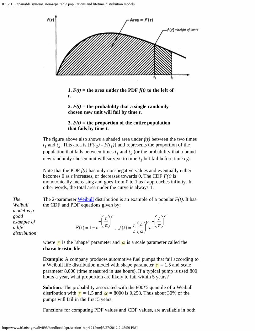
A lifetime distribution model can be any probability density function (orPDF) f(t) defined over the range of time from t = 0 to t = infinity. Thecorresponding cumulative distribution function (or CDF) F(t) is a veryuseful function, as it gives the probability that a randomly selected unit willfail by time t. The figure below shows the relationship between f(t) and F(t)and gives three descriptions of F(t).
8.1.2.1. Repairable systems, non-repairable populations and lifetime distribution models
http://www.itl.nist.gov/div898/handbook/apr/section1/apr121.htm[6/27/2012 2:48:59 PM]
1. F(t) = the area under the PDF f(t) to the left oft.
2. F(t) = the probability that a single randomlychosen new unit will fail by time t.
3. F(t) = the proportion of the entire populationthat fails by time t.
The figure above also shows a shaded area under f(t) between the two timest1 and t2. This area is [F(t2) - F(t1)] and represents the proportion of thepopulation that fails between times t1 and t2 (or the probability that a brandnew randomly chosen unit will survive to time t1 but fail before time t2).
Note that the PDF f(t) has only non-negative values and eventually eitherbecomes 0 as t increases, or decreases towards 0. The CDF F(t) ismonotonically increasing and goes from 0 to 1 as t approaches infinity. Inother words, the total area under the curve is always 1.
TheWeibullmodel is agoodexample ofa lifedistribution
The 2-parameter Weibull distribution is an example of a popular F(t). It hasthe CDF and PDF equations given by:
where is the "shape" parameter and is a scale parameter called thecharacteristic life.
Example: A company produces automotive fuel pumps that fail according toa Weibull life distribution model with shape parameter = 1.5 and scaleparameter 8,000 (time measured in use hours). If a typical pump is used 800hours a year, what proportion are likely to fail within 5 years?
Solution: The probability associated with the 800*5 quantile of a Weibulldistribution with = 1.5 and = 8000 is 0.298. Thus about 30% of thepumps will fail in the first 5 years.
Functions for computing PDF values and CDF values, are available in both

8.1.2.1. Repairable systems, non-repairable populations and lifetime distribution models
http://www.itl.nist.gov/div898/handbook/apr/section1/apr121.htm[6/27/2012 2:48:59 PM]
Dataplot code and R code.

8.1.2.2. Reliability or survival function
http://www.itl.nist.gov/div898/handbook/apr/section1/apr122.htm[6/27/2012 2:49:00 PM]
8. Assessing Product Reliability 8.1. Introduction 8.1.2. What are the basic terms and models used for reliability evaluation?
8.1.2.2. Reliability or survival function
Survival is thecomplementaryevent to failure
The Reliability FunctionR(t), also known as the SurvivalFunction S(t), is defined by:
R(t) = S(t) = the probability a unit survives beyond time t.
Since a unit either fails, or survives, and one of these twomutually exclusive alternatives must occur, we have
R(t) = 1 - F(t), F(t) = 1 - R(t)
Calculations using R(t) often occur when building up fromsingle components to subsystems with many components.For example, if one microprocessor comes from apopulation with reliability function Rm(t) and two of themare used for the CPU in a system, then the system CPUhas a reliability function given by
Rcpu(t) = Rm2(t)
The reliabilityof the system isthe product ofthe reliabilityfunctions ofthecomponents
since both must survive in order for the system to survive.This building up to the system from the individualcomponents will be discussed in detail when we look atthe "Bottom-Up" method. The general rule is: to calculatethe reliability of a system of independent components,multiply the reliability functions of all the componentstogether.
8.1.2.3. Failure (or hazard) rate
http://www.itl.nist.gov/div898/handbook/apr/section1/apr123.htm[6/27/2012 2:49:01 PM]
8. Assessing Product Reliability 8.1. Introduction 8.1.2. What are the basic terms and models used for reliability evaluation?
8.1.2.3. Failure (or hazard) rate
Thefailurerate is therate atwhich thepopulationsurvivorsat anygiveninstant are"fallingover thecliff"
The failure rate is defined for non repairable populations as the(instantaneous) rate of failure for the survivors to time t duringthe next instant of time. It is a rate per unit of time similar inmeaning to reading a car speedometer at a particular instant andseeing 45 mph. The next instant the failure rate may change andthe units that have already failed play no further role since onlythe survivors count.
The failure rate (or hazard rate) is denoted by h(t) and calculatedfrom
The failure rate is sometimes called a "conditional failure rate"since the denominator 1 - F(t) (i.e., the population survivors)converts the expression into a conditional rate, given survivalpast time t.
Since h(t) is also equal to the negative of the derivative ofln{R(t)}, we have the useful identity:
If we let
be the Cumulative Hazard Function, we then have F(t) = 1 - e-
H(t). Two other useful identities that follow from these formulasare:
8.1.2.3. Failure (or hazard) rate
http://www.itl.nist.gov/div898/handbook/apr/section1/apr123.htm[6/27/2012 2:49:01 PM]
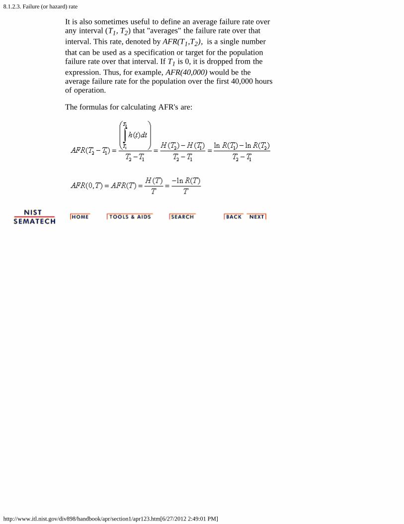
It is also sometimes useful to define an average failure rate overany interval (T1, T2) that "averages" the failure rate over thatinterval. This rate, denoted by AFR(T1,T2), is a single numberthat can be used as a specification or target for the populationfailure rate over that interval. If T1 is 0, it is dropped from theexpression. Thus, for example, AFR(40,000) would be theaverage failure rate for the population over the first 40,000 hoursof operation.
The formulas for calculating AFR's are:

8.1.2.4. "Bathtub" curve
http://www.itl.nist.gov/div898/handbook/apr/section1/apr124.htm[6/27/2012 2:49:01 PM]
8. Assessing Product Reliability 8.1. Introduction 8.1.2. What are the basic terms and models used for reliability evaluation?
8.1.2.4. "Bathtub" curve
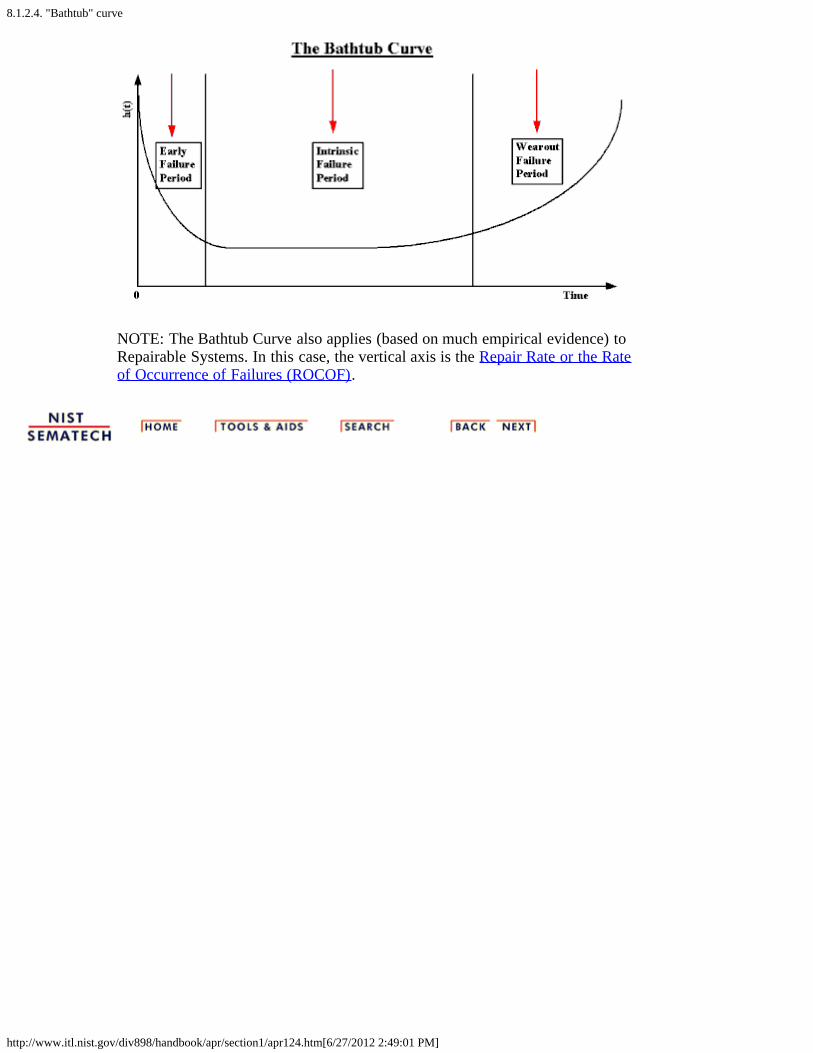
A plot ofthefailurerateovertime formostproductsyields acurvethatlookslike adrawingof abathtub
If enough units from a given population are observed operating and failing overtime, it is relatively easy to compute week-by-week (or month-by-month)estimates of the failure rate h(t). For example, if N12 units survive to start the13th month of life and r13 of them fail during the next month (or 720 hours) oflife, then a simple empirical estimate of h(t) averaged across the 13th month oflife (or between 8640 hours and 9360 hours of age), is given by (r13 / N12 *720). Similar estimates are discussed in detail in the section on Empirical ModelFitting.
Over many years, and across a wide variety of mechanical and electroniccomponents and systems, people have calculated empirical population failurerates as units age over time and repeatedly obtained a graph such as shownbelow. Because of the shape of this failure rate curve, it has become widelyknown as the "Bathtub" curve.
The initial region that begins at time zero when a customer first begins to use theproduct is characterized by a high but rapidly decreasing failure rate. This regionis known as the Early Failure Period (also referred to as Infant MortalityPeriod, from the actuarial origins of the first bathtub curve plots). Thisdecreasing failure rate typically lasts several weeks to a few months.
Next, the failure rate levels off and remains roughly constant for (hopefully) themajority of the useful life of the product. This long period of a level failure rateis known as the Intrinsic Failure Period (also called the Stable FailurePeriod) and the constant failure rate level is called the Intrinsic Failure Rate.Note that most systems spend most of their lifetimes operating in this flatportion of the bathtub curve
Finally, if units from the population remain in use long enough, the failure ratebegins to increase as materials wear out and degradation failures occur at an everincreasing rate. This is the Wearout Failure Period.
8.1.2.4. "Bathtub" curve
http://www.itl.nist.gov/div898/handbook/apr/section1/apr124.htm[6/27/2012 2:49:01 PM]
NOTE: The Bathtub Curve also applies (based on much empirical evidence) toRepairable Systems. In this case, the vertical axis is the Repair Rate or the Rateof Occurrence of Failures (ROCOF).

8.1.2.5. Repair rate or ROCOF
http://www.itl.nist.gov/div898/handbook/apr/section1/apr125.htm[6/27/2012 2:49:02 PM]
8. Assessing Product Reliability 8.1. Introduction 8.1.2. What are the basic terms and models used for reliability evaluation?
8.1.2.5. Repair rate or ROCOF
RepairRatemodels arebased oncountingthecumulativenumber offailuresover time
A different approach is used for modeling the rate ofoccurrence of failure incidences for a repairable system. Inthis chapter, these rates are called repair rates (not to beconfused with the length of time for a repair, which is notdiscussed in this chapter). Time is measured by system power-on-hours from initial turn-on at time zero, to the end ofsystem life. Failures occur as given system ages and thesystem is repaired to a state that may be the same as new, orbetter, or worse. The frequency of repairs may be increasing,decreasing, or staying at a roughly constant rate.
Let N(t) be a counting function that keeps track of thecumulative number of failures a given system has had fromtime zero to time t. N(t) is a step function that jumps up oneevery time a failure occurs and stays at the new level until thenext failure.
Every system will have its own observed N(t) function overtime. If we observed the N(t) curves for a large number ofsimilar systems and "averaged" these curves, we would havean estimate of M(t) = the expected number (average number)of cumulative failures by time t for these systems.
The RepairRate (orROCOF)is themean rateof failuresper unittime
The derivative of M(t), denoted m(t), is defined to be theRepair Rate or the Rate Of Occurrence Of Failures at Timet or ROCOF.
Models for N(t), M(t) and m(t) will be described in the sectionon Repair Rate Models.
8.1.3. What are some common difficulties with reliability data and how are they overcome?
http://www.itl.nist.gov/div898/handbook/apr/section1/apr13.htm[6/27/2012 2:49:03 PM]
8. Assessing Product Reliability 8.1. Introduction
8.1.3. What are some common difficulties withreliability data and how are theyovercome?
TheParadoxofReliabilityAnalysis:The morereliable aproduct is,the harderit is to getthe failuredataneeded to"prove" itis reliable!
There are two closely related problems that are typical withreliability data and not common with most other forms ofstatistical data. These are:
Censoring (when the observation period ends, not allunits have failed - some are survivors)Lack of Failures (if there is too much censoring, eventhough a large number of units may be underobservation, the information in the data is limited due tothe lack of actual failures)
These problems cause considerable practical difficulty whenplanning reliability assessment tests and analyzing failure data.Some solutions are discussed in the next two sections.Typically, the solutions involve making additional assumptionsand using complicated models.

8.1.3.1. Censoring
http://www.itl.nist.gov/div898/handbook/apr/section1/apr131.htm[6/27/2012 2:49:03 PM]
8. Assessing Product Reliability 8.1. Introduction 8.1.3. What are some common difficulties with reliability data and how are they overcome?
8.1.3.1. Censoring
When notall unitson test failwe havecensoreddata
Consider a situation in which we are reliability testing n (non repairable) unitstaken randomly from a population. We are investigating the population todetermine if its failure rate is acceptable. In the typical test scenario, we have afixed time T to run the units to see if they survive or fail. The data obtained arecalled Censored Type I data.
Censored Type I Data
During the T hours of test we observe r failures (where r can be any numberfrom 0 to n). The (exact) failure times are t1, t2, ..., tr and there are (n - r) unitsthat survived the entire T-hour test without failing. Note that T is fixed inadvance and r is random, since we don't know how many failures will occur untilthe test is run. Note also that we assume the exact times of failure are recordedwhen there are failures.
This type of censoring is also called "right censored" data since the times offailure to the right (i.e., larger than T) are missing.
Another (much less common) way to test is to decide in advance that you wantto see exactly r failure times and then test until they occur. For example, youmight put 100 units on test and decide you want to see at least half of them fail.Then r = 50, but T is unknown until the 50th fail occurs. This is called CensoredType II data.
Censored Type II Data
We observe t1, t2, ..., tr, where r is specified in advance. The test ends at time T= tr, and (n-r) units have survived. Again we assume it is possible to observethe exact time of failure for failed units.
Type II censoring has the significant advantage that you know in advance howmany failure times your test will yield - this helps enormously when planningadequate tests. However, an open-ended random test time is generallyimpractical from a management point of view and this type of testing is rarelyseen.
Sometimeswe don'teven knowthe exacttime offailure
Readout or Interval Data
Sometimes exact times of failure are not known; only an interval of time inwhich the failure occurred is recorded. This kind of data is called Readout orInterval data and the situation is shown in the figure below:

8.1.3.1. Censoring
http://www.itl.nist.gov/div898/handbook/apr/section1/apr131.htm[6/27/2012 2:49:03 PM]
.
Multicensored Data
In the most general case, every unit observed yields exactly one of the followingthree types of information:
a run-time if the unit did not fail while under observationan exact failure timean interval of time during which the unit failed.
The units may all have different run-times and/or readout intervals.
Manyspecialmethodshave beendevelopedto handlecensoreddata
How do we handle censored data?
Many statistical methods can be used to fit models and estimate failure rates,even with censored data. In later sections we will discuss the Kaplan-Meierapproach, Probability Plotting, Hazard Plotting, Graphical Estimation, andMaximum Likelihood Estimation.
Separating out Failure Modes
Note that when a data set consists of failure times that can be sorted into severaldifferent failure modes, it is possible (and often necessary) to analyze and modeleach mode separately. Consider all failures due to modes other than the onebeing analyzed as censoring times, with the censored run-time equal to the timeit failed due to the different (independent) failure mode. This is discussed furtherin the competing risk section and later analysis sections.

8.1.3.2. Lack of failures
http://www.itl.nist.gov/div898/handbook/apr/section1/apr132.htm[6/27/2012 2:49:04 PM]
8. Assessing Product Reliability 8.1. Introduction 8.1.3. What are some common difficulties with reliability data and how are they overcome?
8.1.3.2. Lack of failures
Failuredata isneeded toaccuratelyassess andimprovereliability- thisposesproblemswhentestinghighlyreliableparts
When fitting models and estimating failure rates fromreliability data, the precision of the estimates (as measured bythe width of the confidence intervals) tends to vary inverselywith the square root of the number of failures observed - notthe number of units on test or the length of the test. In otherwords, a test where 5 fail out of a total of 10 on test givesmore information than a test with 1000 units but only 2failures.
Since the number of failures r is critical, and not the samplesize n on test, it becomes increasingly difficult to assess thefailure rates of highly reliable components. Parts like memorychips, that in typical use have failure rates measured in partsper million per thousand hours, will have few or no failureswhen tested for reasonable time periods with affordablesample sizes. This gives little or no information foraccomplishing the two primary purposes of reliability testing,namely:
accurately assessing population failure ratesobtaining failure mode information to feedback forproduct improvement.
Testing atmuchhigherthantypicalstressescan yieldfailuresbut modelsare thenneeded torelatethese backto usestress
How can tests be designed to overcome an expected lack offailures?
The answer is to make failures occur by testing at much higherstresses than the units would normally see in their intendedapplication. This creates a new problem: how can thesefailures at higher-than-normal stresses be related to whatwould be expected to happen over the course of many years atnormal use stresses? The models that relate high stressreliability to normal use reliability are called accelerationmodels.

8.1.3.2. Lack of failures
http://www.itl.nist.gov/div898/handbook/apr/section1/apr132.htm[6/27/2012 2:49:04 PM]

8.1.4. What is "physical acceleration" and how do we model it?
http://www.itl.nist.gov/div898/handbook/apr/section1/apr14.htm[6/27/2012 2:49:05 PM]
8. Assessing Product Reliability 8.1. Introduction
8.1.4. What is "physical acceleration" and howdo we model it?
Whenchangingstress isequivalent tomultiplyingtime to failby aconstant, wehave true(physical)acceleration
Physical Acceleration (sometimes called TrueAcceleration or just Acceleration) means that operating aunit at high stress (i.e., higher temperature or voltage orhumidity or duty cycle, etc.) produces the same failures thatwould occur at typical-use stresses, except that they happenmuch quicker.
Failure may be due to mechanical fatigue, corrosion,chemical reaction, diffusion, migration, etc. These are thesame causes of failure under normal stress; the time scale issimply different.
AnAccelerationFactor is theconstantmultiplierbetween thetwo stresslevels
When there is true acceleration, changing stress is equivalentto transforming the time scale used to record when failuresoccur. The transformations commonly used are linear,which means that time-to-fail at high stress just has to bemultiplied by a constant (the acceleration factor) to obtainthe equivalent time-to-fail at use stress.
We use the following notation:
ts = time-to-fail at stress tu = corresponding time-to-fail atuse
Fs(t) = CDF at stress Fu(t) = CDF at usefs(t) = PDF at stress fu(t) = PDF at usehs(t) = failure rate atstress
hu(t) = failure rate at use
Then, an acceleration factor AF between stress and usemeans the following relationships hold:
Linear Acceleration Relationships
Time-to-Fail tu = AF × tsFailure Probability Fu(t) = Fs(t/AF)
Reliability Ru(t) = Rs(t/AF)
PDF or Density Function fu(t) = (1/AF)fs(t/AF)
Failure Rate hu(t) = (1/AF) hs(t/AF)

8.1.4. What is "physical acceleration" and how do we model it?
http://www.itl.nist.gov/div898/handbook/apr/section1/apr14.htm[6/27/2012 2:49:05 PM]
Each failuremode has itsownaccelerationfactor
Failure datashould beseparated byfailure modewhenanalyzed, ifaccelerationis relevant
Probabilityplots of datafromdifferentstress cellshave thesame slope(if there isacceleration)
Note: Acceleration requires that there be a stress dependentphysical process causing change or degradation that leads tofailure. In general, different failure modes will be affecteddifferently by stress and have different acceleration factors.Therefore, it is unlikely that a single acceleration factor willapply to more than one failure mechanism. In general,different failure modes will be affected differently by stressand have different acceleration factors. Separate outdifferent types of failure when analyzing failure data.
Also, a consequence of the linear acceleration relationshipsshown above (which follows directly from "trueacceleration") is the following:
The Shape Parameter for the key lifedistribution models (Weibull, Lognormal) doesnot change for units operating under differentstresses. Probability plots of data from differentstress cells will line up roughly parallel.
These distributions and probability plotting will bediscussed in later sections.

8.1.5. What are some common acceleration models?
http://www.itl.nist.gov/div898/handbook/apr/section1/apr15.htm[6/27/2012 2:49:06 PM]
8. Assessing Product Reliability 8.1. Introduction
8.1.5. What are some common accelerationmodels?
Accelerationmodelspredict timeto fail as afunction ofstress
Acceleration factors show how time-to-fail at a particularoperating stress level (for one failure mode or mechanism)can be used to predict the equivalent time to fail at adifferent operating stress level.
A model that predicts time-to-fail as a function of stresswould be even better than a collection of accelerationfactors. If we write tf = G(S), with G(S) denoting the modelequation for an arbitrary stress level S, then the accelerationfactor between two stress levels S1 and S2 can be evaluatedsimply by AF = G(S1)/G(S2). Now we can test at the higherstress S2, obtain a sufficient number of failures to fit lifedistribution models and evaluate failure rates, and use theLinear Acceleration Relationships Table to predict what willoccur at the lower use stress S1.
A model that predicts time-to-fail as a function of operatingstresses is known as an acceleration model.
Accelerationmodels areoftenderivedfromphysics orkineticsmodelsrelated tothe failuremechanism
Acceleration models are usually based on the physics orchemistry underlying a particular failure mechanism.Successful empirical models often turn out to beapproximations of complicated physics or kinetics models,when the theory of the failure mechanism is betterunderstood. The following sections will consider a variety ofpowerful and useful models:
ArrheniusEyringOther Models
8.1.5.1. Arrhenius
http://www.itl.nist.gov/div898/handbook/apr/section1/apr151.htm[6/27/2012 2:49:06 PM]
8. Assessing Product Reliability 8.1. Introduction 8.1.5. What are some common acceleration models?
8.1.5.1. Arrhenius
TheArrheniusmodelpredictsfailureaccelerationdue totemperatureincrease
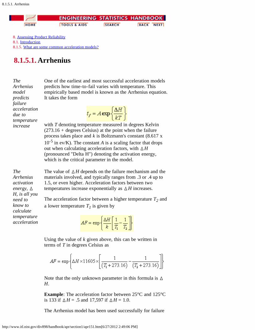
One of the earliest and most successful acceleration modelspredicts how time-to-fail varies with temperature. Thisempirically based model is known as the Arrhenius equation.It takes the form
with T denoting temperature measured in degrees Kelvin(273.16 + degrees Celsius) at the point when the failureprocess takes place and k is Boltzmann's constant (8.617 x10⁻⁵ in ev/K). The constant A is a scaling factor that dropsout when calculating acceleration factors, with H(pronounced "Delta H") denoting the activation energy,which is the critical parameter in the model.
TheArrheniusactivationenergy, H, is all youneed toknow tocalculatetemperatureacceleration
The value of H depends on the failure mechanism and thematerials involved, and typically ranges from .3 or .4 up to1.5, or even higher. Acceleration factors between twotemperatures increase exponentially as H increases.
The acceleration factor between a higher temperature T2 anda lower temperature T1 is given by
Using the value of k given above, this can be written interms of T in degrees Celsius as
Note that the only unknown parameter in this formula is H.
Example: The acceleration factor between 25°C and 125°Cis 133 if H = .5 and 17,597 if H = 1.0.
The Arrhenius model has been used successfully for failure

8.1.5.1. Arrhenius
http://www.itl.nist.gov/div898/handbook/apr/section1/apr151.htm[6/27/2012 2:49:06 PM]
mechanisms that depend on chemical reactions, diffusionprocesses or migration processes. This covers many of thenon mechanical (or non material fatigue) failure modes thatcause electronic equipment failure.

8.1.5.2. Eyring
http://www.itl.nist.gov/div898/handbook/apr/section1/apr152.htm[6/27/2012 2:49:07 PM]
8. Assessing Product Reliability 8.1. Introduction 8.1.5. What are some common acceleration models?
8.1.5.2. Eyring
The Eyringmodel has atheoreticalbasis inchemistryand quantummechanicsand can beused tomodelaccelerationwhen manystresses areinvolved
Henry Eyring's contributions to chemical reaction rate theoryhave led to a very general and powerful model foracceleration known as the Eyring Model. This model hasseveral key features:
It has a theoretical basis from chemistry and quantummechanics.If a chemical process (chemical reaction, diffusion,corrosion, migration, etc.) is causing degradationleading to failure, the Eyring model describes how therate of degradation varies with stress or, equivalently,how time to failure varies with stress.The model includes temperature and can be expandedto include other relevant stresses.The temperature term by itself is very similar to theArrhenius empirical model, explaining why that modelhas been so successful in establishing the connectionbetween the H parameter and the quantum theoryconcept of "activation energy needed to cross anenergy barrier and initiate a reaction".
The model for temperature and one additional stress takesthe general form:
for which S1 could be some function of voltage or current orany other relevant stress and the parameters , H, B, andC determine acceleration between stress combinations. Aswith the Arrhenius Model, k is Boltzmann's constant andtemperature is in degrees Kelvin.
If we want to add an additional non-thermal stress term, themodel becomes
and as many stresses as are relevant can be included byadding similar terms.

8.1.5.2. Eyring
http://www.itl.nist.gov/div898/handbook/apr/section1/apr152.htm[6/27/2012 2:49:07 PM]
Models withmultiplestressesgenerallyhave nointeractionterms -which meansyou canmultiplyaccelerationfactors dueto differentstresses
Note that the general Eyring model includes terms that havestress and temperature interactions (in other words, theeffect of changing temperature varies, depending on thelevels of other stresses). Most models in actual use do notinclude any interaction terms, so that the relative change inacceleration factors when only one stress changes does notdepend on the level of the other stresses.
In models with no interaction, you can compute accelerationfactors for each stress and multiply them together. Thiswould not be true if the physical mechanism requiredinteraction terms - but, at least to first approximations, itseems to work for most examples in the literature.
The Eyringmodel canalso be usedto modelrate ofdegradationleading tofailure as afunction ofstress
Advantages of the Eyring Model
Can handle many stresses.Can be used to model degradation data as well asfailure data.The H parameter has a physical meaning and hasbeen studied and estimated for many well knownfailure mechanisms and materials.
In practice,the EyringModel isusually toocomplicatedto use in itsmost generalform andmust be"customized"or simplifiedfor anyparticularfailuremechanism
Disadvantages of the Eyring Model
Even with just two stresses, there are 5 parameters toestimate. Each additional stress adds 2 more unknownparameters.Many of the parameters may have only a second-order effect. For example, setting = 0 works quitewell since the temperature term then becomes thesame as in the Arrhenius model. Also, the constants Cand E are only needed if there is a significanttemperature interaction effect with respect to the otherstresses.The form in which the other stresses appear is notspecified by the general model and may varyaccording to the particular failure mechanism. In otherwords, S1 may be voltage or ln (voltage) or someother function of voltage.
Many well-known models are simplified versions of theEyring model with appropriate functions of relevant stresseschosen for S1 and S2. Some of these will be shown in theOther Models section. The trick is to find the rightsimplification to use for a particular failure mechanism.

8.1.5.3. Other models
http://www.itl.nist.gov/div898/handbook/apr/section1/apr153.htm[6/27/2012 2:49:08 PM]
8. Assessing Product Reliability 8.1. Introduction 8.1.5. What are some common acceleration models?
8.1.5.3. Other models
Manyuseful 1, 2and 3stressmodels aresimpleEyringmodels.Six aredescribed
This section will discuss several acceleration models whosesuccessful use has been described in the literature.
The (Inverse) Power Rule for VoltageThe Exponential Voltage ModelTwo Temperature/Voltage ModelsThe Electromigration ModelThree Stress Models (Temperature, Voltage andHumidity)The Coffin-Manson Mechanical Crack Growth Model
The (Inverse) Power Rule for Voltage
This model, used for capacitors, has only voltage dependencyand takes the form:
This is a very simplified Eyring model with , H, and C all0, and S = lnV, and = -B.
The Exponential Voltage Model
In some cases, voltage dependence is modeled better with anexponential model:
Two Temperature/Voltage Models
Temperature/Voltage models are common in the literature andtake one of the two forms given below:
8.1.5.3. Other models
http://www.itl.nist.gov/div898/handbook/apr/section1/apr153.htm[6/27/2012 2:49:08 PM]
Again, these are just simplified two stress Eyring models withthe appropriate choice of constants and functions of voltage.
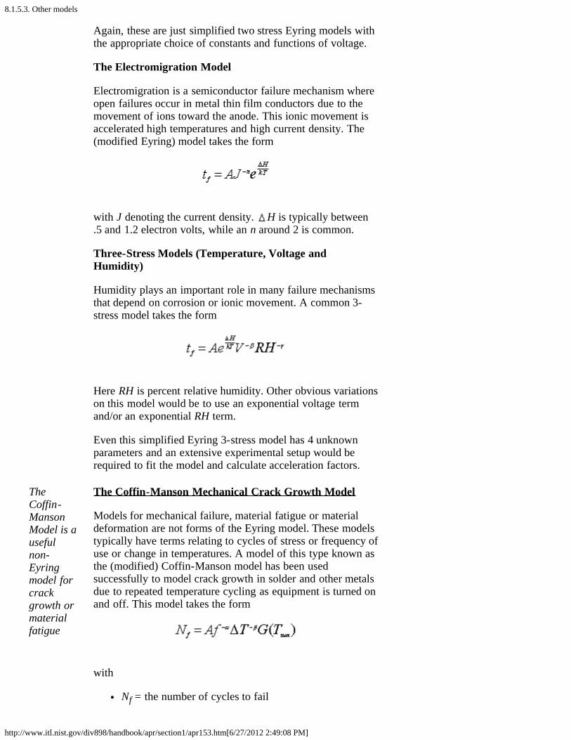
The Electromigration Model
Electromigration is a semiconductor failure mechanism whereopen failures occur in metal thin film conductors due to themovement of ions toward the anode. This ionic movement isaccelerated high temperatures and high current density. The(modified Eyring) model takes the form
with J denoting the current density. H is typically between.5 and 1.2 electron volts, while an n around 2 is common.
Three-Stress Models (Temperature, Voltage andHumidity)
Humidity plays an important role in many failure mechanismsthat depend on corrosion or ionic movement. A common 3-stress model takes the form
Here RH is percent relative humidity. Other obvious variationson this model would be to use an exponential voltage termand/or an exponential RH term.
Even this simplified Eyring 3-stress model has 4 unknownparameters and an extensive experimental setup would berequired to fit the model and calculate acceleration factors.
TheCoffin-MansonModel is ausefulnon-Eyringmodel forcrackgrowth ormaterialfatigue
The Coffin-Manson Mechanical Crack Growth Model
Models for mechanical failure, material fatigue or materialdeformation are not forms of the Eyring model. These models typically have terms relating to cycles of stress or frequency ofuse or change in temperatures. A model of this type known asthe (modified) Coffin-Manson model has been usedsuccessfully to model crack growth in solder and other metalsdue to repeated temperature cycling as equipment is turned onand off. This model takes the form
with
Nf = the number of cycles to fail

8.1.5.3. Other models
http://www.itl.nist.gov/div898/handbook/apr/section1/apr153.htm[6/27/2012 2:49:08 PM]
f = the cycling frequencyT = the temperature range during a cycle
and G(Tmax) is an Arrhenius term evaluated at the maximumtemperature reached in each cycle.
Typical values for the cycling frequency exponent and thetemperature range exponent are around -1/3 and 2,respectively (note that reducing the cycling frequency reducesthe number of cycles to failure). The H activation energyterm in G(Tmax) is around 1.25.

8.1.6. What are the basic lifetime distribution models used for non-repairable populations?
http://www.itl.nist.gov/div898/handbook/apr/section1/apr16.htm[6/27/2012 2:49:09 PM]
8. Assessing Product Reliability 8.1. Introduction
8.1.6. What are the basic lifetime distributionmodels used for non-repairablepopulations?
A handfulof lifetimedistributionmodelshaveenjoyedgreatpracticalsuccess
There are a handful of parametric models that havesuccessfully served as population models for failure timesarising from a wide range of products and failuremechanisms. Sometimes there are probabilistic argumentsbased on the physics of the failure mode that tend to justifythe choice of model. Other times the model is used solelybecause of its empirical success in fitting actual failure data.
Seven models will be described in this section:
1. Exponential2. Weibull3. Extreme Value 4. Lognormal5. Gamma 6. Birnbaum-Saunders7. Proportional hazards
8.1.6.1. Exponential
http://www.itl.nist.gov/div898/handbook/apr/section1/apr161.htm[6/27/2012 2:49:10 PM]
8. Assessing Product Reliability 8.1. Introduction 8.1.6. What are the basic lifetime distribution models used for non-repairable populations?
8.1.6.1. Exponential
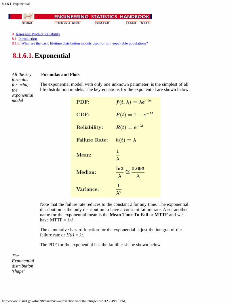
All the keyformulasfor usingtheexponentialmodel
Formulas and Plots
The exponential model, with only one unknown parameter, is the simplest of alllife distribution models. The key equations for the exponential are shown below:
Note that the failure rate reduces to the constant λ for any time. The exponentialdistribution is the only distribution to have a constant failure rate. Also, anothername for the exponential mean is the Mean Time To Fail or MTTF and wehave MTTF = 1/λ.
The cumulative hazard function for the exponential is just the integral of thefailure rate or H(t) = λt.
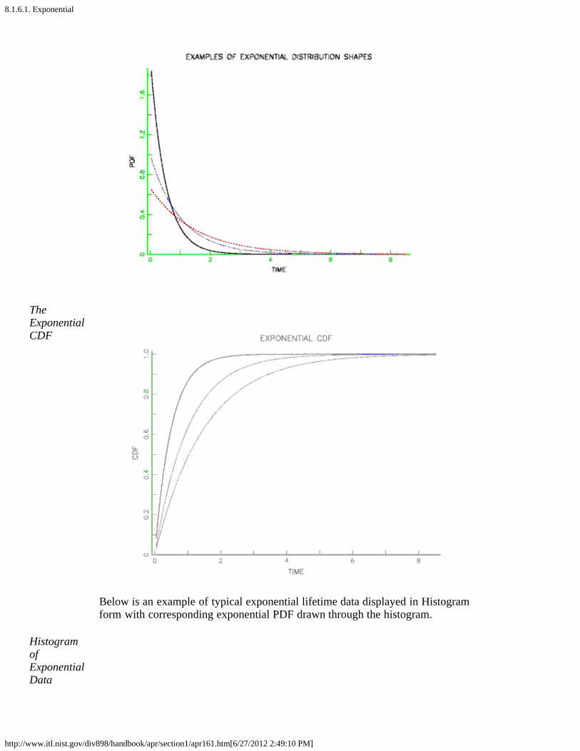
The PDF for the exponential has the familiar shape shown below.
TheExponentialdistribution'shape'
8.1.6.1. Exponential
http://www.itl.nist.gov/div898/handbook/apr/section1/apr161.htm[6/27/2012 2:49:10 PM]
TheExponentialCDF
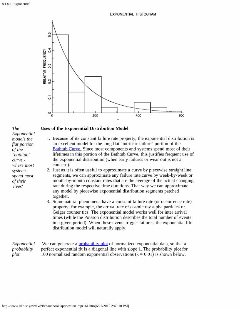
Below is an example of typical exponential lifetime data displayed in Histogramform with corresponding exponential PDF drawn through the histogram.
HistogramofExponentialData
8.1.6.1. Exponential
http://www.itl.nist.gov/div898/handbook/apr/section1/apr161.htm[6/27/2012 2:49:10 PM]
TheExponentialmodels theflat portionof the"bathtub"curve -where mostsystemsspend mostof their'lives'
Uses of the Exponential Distribution Model
1. Because of its constant failure rate property, the exponential distribution isan excellent model for the long flat "intrinsic failure" portion of theBathtub Curve. Since most components and systems spend most of theirlifetimes in this portion of the Bathtub Curve, this justifies frequent use ofthe exponential distribution (when early failures or wear out is not aconcern).
2. Just as it is often useful to approximate a curve by piecewise straight linesegments, we can approximate any failure rate curve by week-by-week ormonth-by-month constant rates that are the average of the actual changingrate during the respective time durations. That way we can approximateany model by piecewise exponential distribution segments patchedtogether.
3. Some natural phenomena have a constant failure rate (or occurrence rate)property; for example, the arrival rate of cosmic ray alpha particles orGeiger counter tics. The exponential model works well for inter arrivaltimes (while the Poisson distribution describes the total number of eventsin a given period). When these events trigger failures, the exponential lifedistribution model will naturally apply.
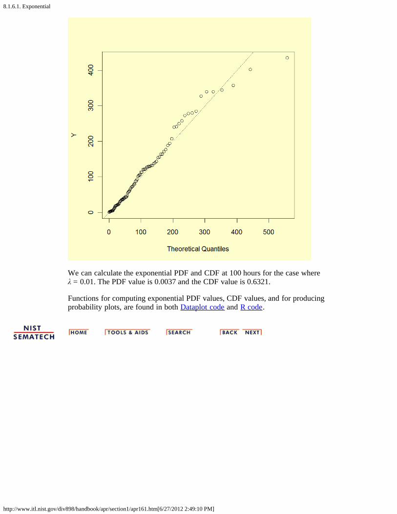
Exponentialprobabilityplot
We can generate a probability plot of normalized exponential data, so that aperfect exponential fit is a diagonal line with slope 1. The probability plot for100 normalized random exponential observations (λ = 0.01) is shown below.
8.1.6.1. Exponential
http://www.itl.nist.gov/div898/handbook/apr/section1/apr161.htm[6/27/2012 2:49:10 PM]
We can calculate the exponential PDF and CDF at 100 hours for the case whereλ = 0.01. The PDF value is 0.0037 and the CDF value is 0.6321.
Functions for computing exponential PDF values, CDF values, and for producingprobability plots, are found in both Dataplot code and R code.

8.1.6.2. Weibull
http://www.itl.nist.gov/div898/handbook/apr/section1/apr162.htm[6/27/2012 2:49:11 PM]
8. Assessing Product Reliability 8.1. Introduction 8.1.6. What are the basic lifetime distribution models used for non-repairable populations?
8.1.6.2. Weibull
WeibullFormulas
Formulas and Plots
The Weibull is a very flexible life distribution model with two parameters. It has CDF andPDF and other key formulas given by:
with α the scale parameter (the Characteristic Life), γ (gamma) the Shape Parameter, and Γis the Gamma function with Γ(N) = (N-1)! for integer N.
The cumulative hazard function for the Weibull is the integral of the failure rate or
A more general three-parameter form of the Weibull includes an additional waiting timeparameter µ (sometimes called a shift or location parameter). The formulas for the 3-parameter Weibull are easily obtained from the above formulas by replacing t by (t - µ)wherever t appears. No failure can occur before µ hours, so the time scale starts at µ, and not0. If a shift parameter µ is known (based, perhaps, on the physics of the failure mode), then allyou have to do is subtract µ from all the observed failure times and/or readout times and
8.1.6.2. Weibull
http://www.itl.nist.gov/div898/handbook/apr/section1/apr162.htm[6/27/2012 2:49:11 PM]
analyze the resulting shifted data with a two-parameter Weibull.
NOTE: Various texts and articles in the literature use a variety of different symbols for thesame Weibull parameters. For example, the characteristic life is sometimes called c (ν = nu orη = eta) and the shape parameter is also called m (or β = beta). To add to the confusion, somesoftware uses β as the characteristic life parameter and α as the shape parameter. Someauthors even parameterize the density function differently, using a scale parameter .
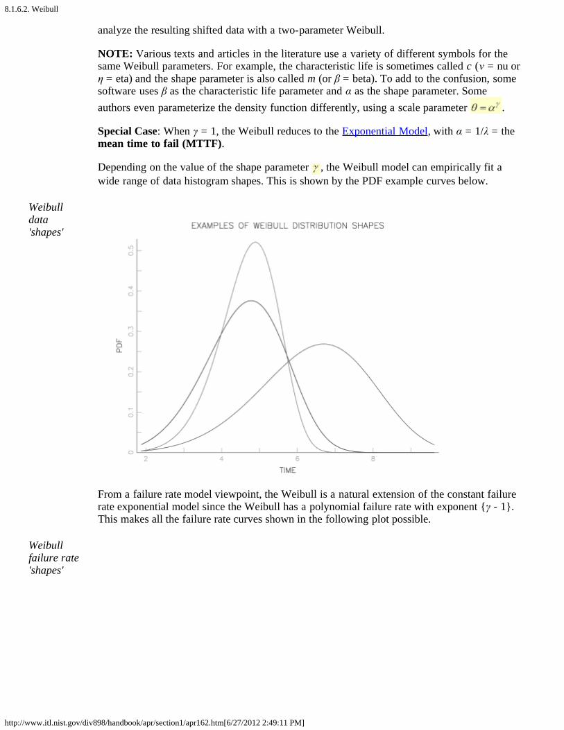
Special Case: When γ = 1, the Weibull reduces to the Exponential Model, with α = 1/λ = themean time to fail (MTTF).
Depending on the value of the shape parameter , the Weibull model can empirically fit awide range of data histogram shapes. This is shown by the PDF example curves below.
Weibulldata'shapes'
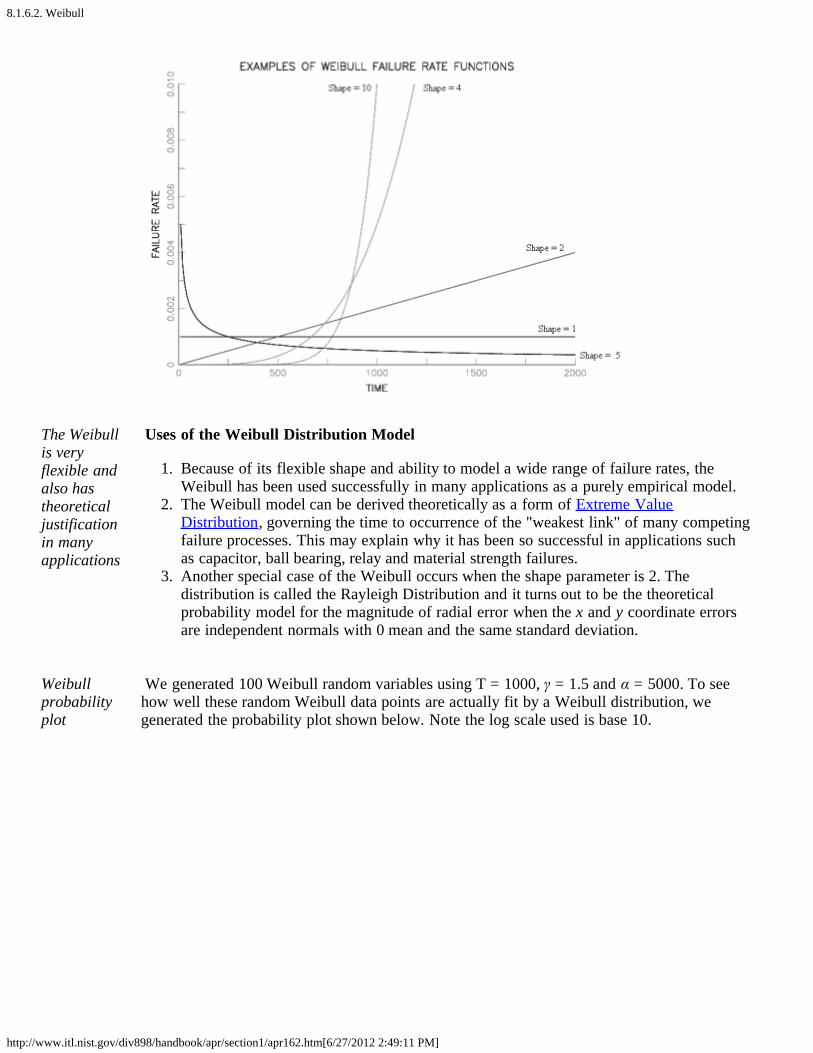
From a failure rate model viewpoint, the Weibull is a natural extension of the constant failurerate exponential model since the Weibull has a polynomial failure rate with exponent {γ - 1}.This makes all the failure rate curves shown in the following plot possible.
Weibullfailure rate'shapes'
8.1.6.2. Weibull
http://www.itl.nist.gov/div898/handbook/apr/section1/apr162.htm[6/27/2012 2:49:11 PM]
The Weibullis veryflexible andalso hastheoreticaljustificationin manyapplications
Uses of the Weibull Distribution Model
1. Because of its flexible shape and ability to model a wide range of failure rates, theWeibull has been used successfully in many applications as a purely empirical model.
2. The Weibull model can be derived theoretically as a form of Extreme ValueDistribution, governing the time to occurrence of the "weakest link" of many competingfailure processes. This may explain why it has been so successful in applications suchas capacitor, ball bearing, relay and material strength failures.
3. Another special case of the Weibull occurs when the shape parameter is 2. Thedistribution is called the Rayleigh Distribution and it turns out to be the theoreticalprobability model for the magnitude of radial error when the x and y coordinate errorsare independent normals with 0 mean and the same standard deviation.
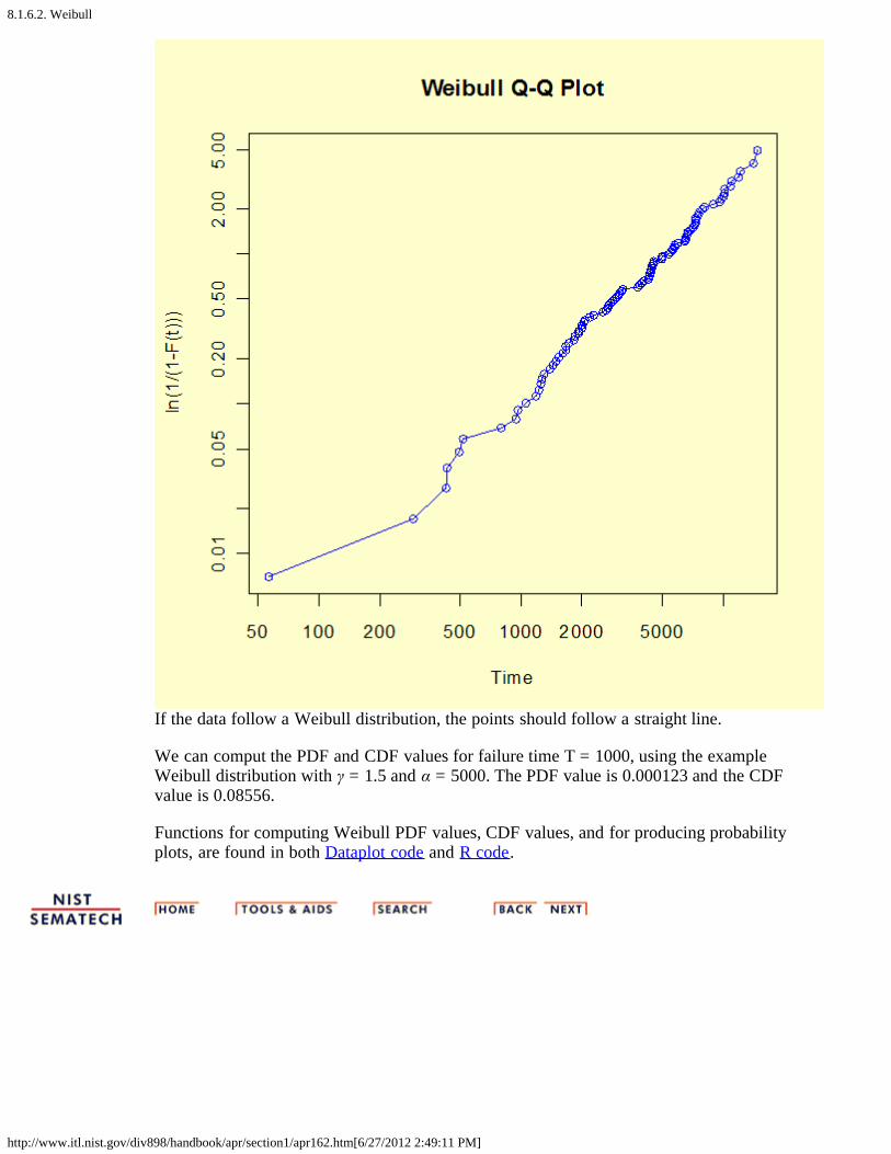
Weibullprobabilityplot
We generated 100 Weibull random variables using T = 1000, γ = 1.5 and α = 5000. To seehow well these random Weibull data points are actually fit by a Weibull distribution, wegenerated the probability plot shown below. Note the log scale used is base 10.
8.1.6.2. Weibull
http://www.itl.nist.gov/div898/handbook/apr/section1/apr162.htm[6/27/2012 2:49:11 PM]
If the data follow a Weibull distribution, the points should follow a straight line.
We can comput the PDF and CDF values for failure time T = 1000, using the exampleWeibull distribution with γ = 1.5 and α = 5000. The PDF value is 0.000123 and the CDFvalue is 0.08556.
Functions for computing Weibull PDF values, CDF values, and for producing probabilityplots, are found in both Dataplot code and R code.
8.1.6.3. Extreme value distributions
http://www.itl.nist.gov/div898/handbook/apr/section1/apr163.htm[6/27/2012 2:49:12 PM]
8. Assessing Product Reliability 8.1. Introduction 8.1.6. What are the basic lifetime distribution models used for non-repairable populations?
8.1.6.3. Extreme value distributions
The ExtremeValueDistributionusuallyrefers to thedistributionof theminimum ofa largenumber ofunboundedrandomobservations
Description, Formulas and Plots
We have already referred to Extreme Value Distributions when describing the uses of theWeibull distribution. Extreme value distributions are the limiting distributions for theminimum or the maximum of a very large collection of random observations from the samearbitrary distribution. Gumbel (1958) showed that for any well-behaved initial distribution(i.e., F(x) is continuous and has an inverse), only a few models are needed, depending onwhether you are interested in the maximum or the minimum, and also if the observations arebounded above or below.
In the context of reliability modeling, extreme value distributions for the minimum arefrequently encountered. For example, if a system consists of n identical components in series,and the system fails when the first of these components fails, then system failure times are theminimum of n random component failure times. Extreme value theory says that, independentof the choice of component model, the system model will approach a Weibull as n becomeslarge. The same reasoning can also be applied at a component level, if the component failureoccurs when the first of many similar competing failure processes reaches a critical level.
The distribution often referred to as the Extreme Value Distribution (Type I) is the limitingdistribution of the minimum of a large number of unbounded identically distributed randomvariables. The PDF and CDF are given by:
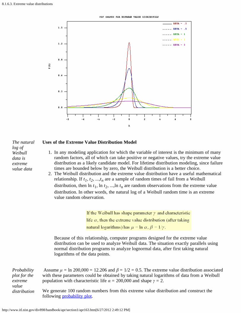
ExtremeValueDistributionformulasand PDFshapes
If the x values are bounded below (as is the case with times of failure) then the limitingdistribution is the Weibull. Formulas and uses of the Weibull have already been discussed.
PDF Shapes for the (minimum) Extreme Value Distribution (Type I) are shown in thefollowing figure.
8.1.6.3. Extreme value distributions
http://www.itl.nist.gov/div898/handbook/apr/section1/apr163.htm[6/27/2012 2:49:12 PM]
The naturallog ofWeibulldata isextremevalue data
Uses of the Extreme Value Distribution Model
1. In any modeling application for which the variable of interest is the minimum of manyrandom factors, all of which can take positive or negative values, try the extreme valuedistribution as a likely candidate model. For lifetime distribution modeling, since failuretimes are bounded below by zero, the Weibull distribution is a better choice.
2. The Weibull distribution and the extreme value distribution have a useful mathematicalrelationship. If t1, t2, ...,tn are a sample of random times of fail from a Weibulldistribution, then ln t1, ln t2, ...,ln tn are random observations from the extreme valuedistribution. In other words, the natural log of a Weibull random time is an extremevalue random observation.
Because of this relationship, computer programs designed for the extreme valuedistribution can be used to analyze Weibull data. The situation exactly parallels usingnormal distribution programs to analyze lognormal data, after first taking naturallogarithms of the data points.
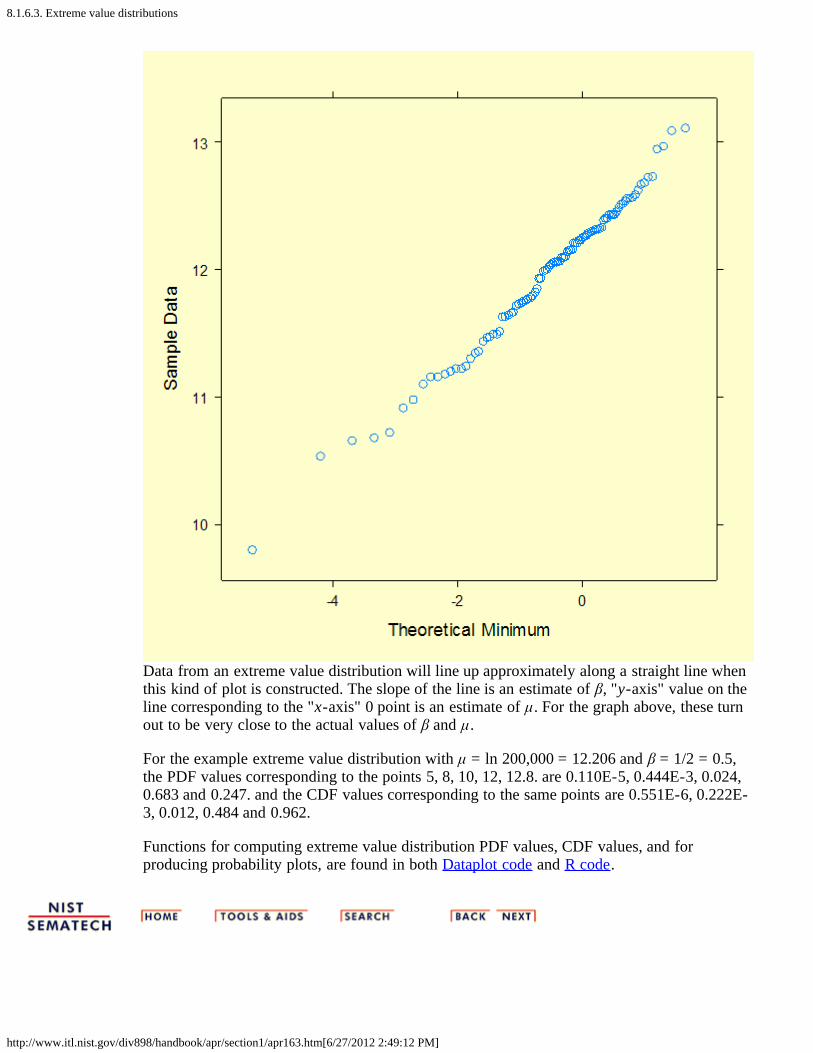
Probabilityplot for theextremevaluedistribution
Assume μ = ln 200,000 = 12.206 and β = 1/2 = 0.5. The extreme value distribution associatedwith these parameters could be obtained by taking natural logarithms of data from a Weibullpopulation with characteristic life α = 200,000 and shape γ = 2.
We generate 100 random numbers from this extreme value distribution and construct thefollowing probability plot.
8.1.6.3. Extreme value distributions
http://www.itl.nist.gov/div898/handbook/apr/section1/apr163.htm[6/27/2012 2:49:12 PM]
Data from an extreme value distribution will line up approximately along a straight line whenthis kind of plot is constructed. The slope of the line is an estimate of β, "y-axis" value on theline corresponding to the "x-axis" 0 point is an estimate of μ. For the graph above, these turnout to be very close to the actual values of β and μ.
For the example extreme value distribution with μ = ln 200,000 = 12.206 and β = 1/2 = 0.5,the PDF values corresponding to the points 5, 8, 10, 12, 12.8. are 0.110E-5, 0.444E-3, 0.024,0.683 and 0.247. and the CDF values corresponding to the same points are 0.551E-6, 0.222E-3, 0.012, 0.484 and 0.962.
Functions for computing extreme value distribution PDF values, CDF values, and forproducing probability plots, are found in both Dataplot code and R code.

8.1.6.4. Lognormal
http://www.itl.nist.gov/div898/handbook/apr/section1/apr164.htm[6/27/2012 2:49:13 PM]
8. Assessing Product Reliability 8.1. Introduction 8.1.6. What are the basic lifetime distribution models used for non-repairable populations?
8.1.6.4. Lognormal
LognormalFormulas andrelationshipto the normaldistribution
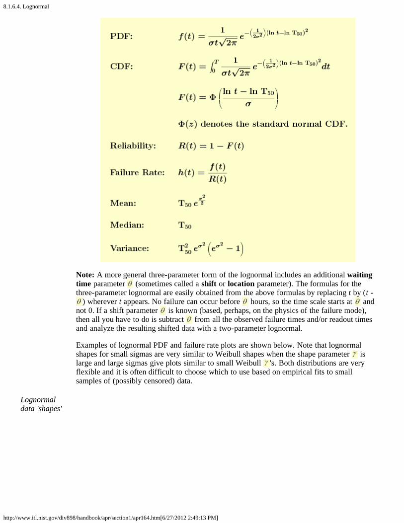
Formulas and Plots
The lognormal life distribution, like the Weibull, is a very flexible model that can empiricallyfit many types of failure data. The two-parameter form has parameters σ is the shapeparameter and T50 is the median (a scale parameter).
Note: If time to failure, tf, has a lognormal distribution, then the (natural) logarithm of time tofailure has a normal distribution with mean µ = ln T50 and standard deviation σ. This makeslognormal data convenient to work with; just take natural logarithms of all the failure timesand censoring times and analyze the resulting normal data. Later on, convert back to real timeand lognormal parameters using σ as the lognormal shape and T50 = eµ as the (median) scaleparameter.
Below is a summary of the key formulas for the lognormal.
8.1.6.4. Lognormal
http://www.itl.nist.gov/div898/handbook/apr/section1/apr164.htm[6/27/2012 2:49:13 PM]
Note: A more general three-parameter form of the lognormal includes an additional waitingtime parameter (sometimes called a shift or location parameter). The formulas for thethree-parameter lognormal are easily obtained from the above formulas by replacing t by (t -
) wherever t appears. No failure can occur before hours, so the time scale starts at andnot 0. If a shift parameter is known (based, perhaps, on the physics of the failure mode),then all you have to do is subtract from all the observed failure times and/or readout timesand analyze the resulting shifted data with a two-parameter lognormal.
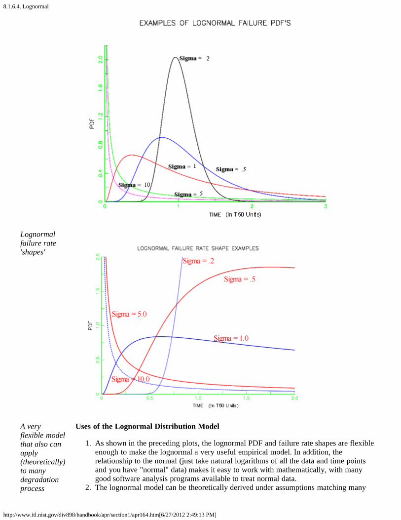
Examples of lognormal PDF and failure rate plots are shown below. Note that lognormalshapes for small sigmas are very similar to Weibull shapes when the shape parameter islarge and large sigmas give plots similar to small Weibull 's. Both distributions are veryflexible and it is often difficult to choose which to use based on empirical fits to smallsamples of (possibly censored) data.
Lognormaldata 'shapes'
8.1.6.4. Lognormal
http://www.itl.nist.gov/div898/handbook/apr/section1/apr164.htm[6/27/2012 2:49:13 PM]
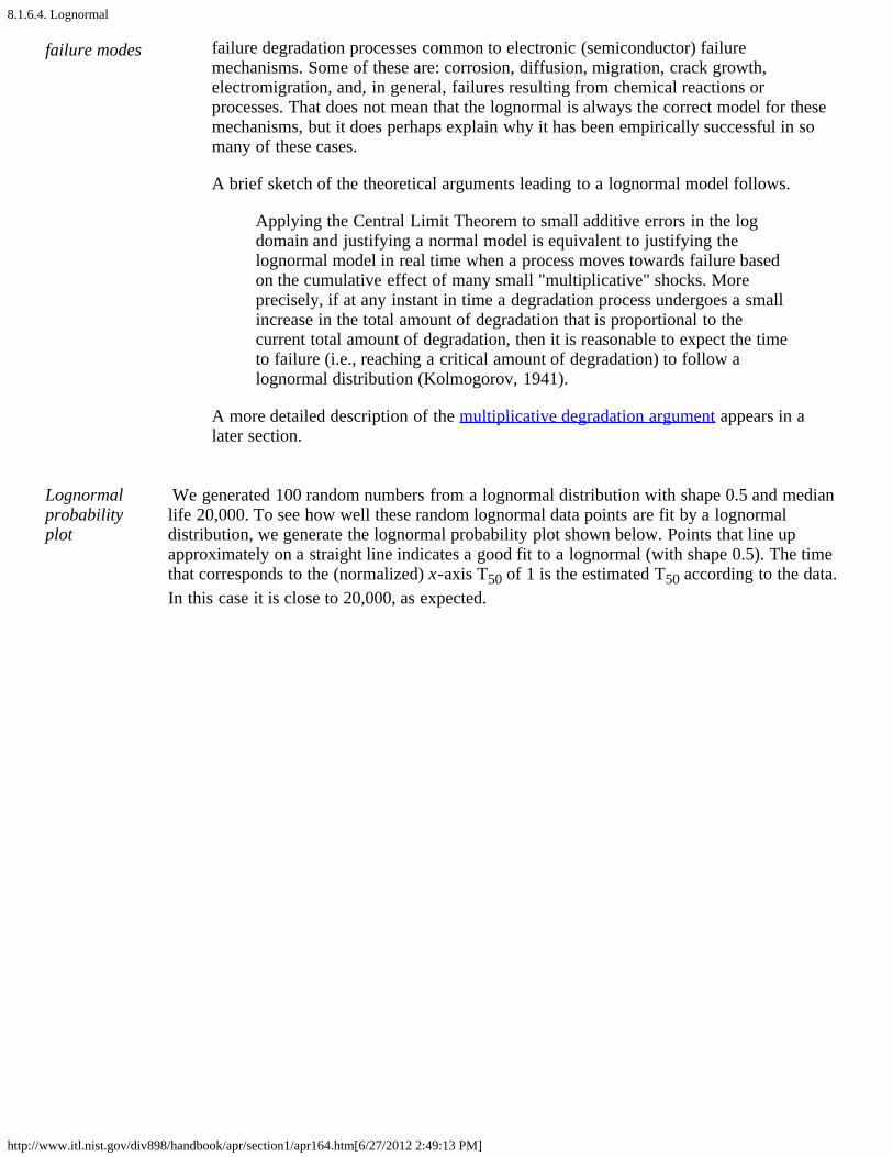
Lognormalfailure rate'shapes'
A veryflexible modelthat also canapply(theoretically)to manydegradationprocess
Uses of the Lognormal Distribution Model
1. As shown in the preceding plots, the lognormal PDF and failure rate shapes are flexibleenough to make the lognormal a very useful empirical model. In addition, therelationship to the normal (just take natural logarithms of all the data and time pointsand you have "normal" data) makes it easy to work with mathematically, with manygood software analysis programs available to treat normal data.
2. The lognormal model can be theoretically derived under assumptions matching many
8.1.6.4. Lognormal
http://www.itl.nist.gov/div898/handbook/apr/section1/apr164.htm[6/27/2012 2:49:13 PM]
failure modes failure degradation processes common to electronic (semiconductor) failuremechanisms. Some of these are: corrosion, diffusion, migration, crack growth,electromigration, and, in general, failures resulting from chemical reactions orprocesses. That does not mean that the lognormal is always the correct model for thesemechanisms, but it does perhaps explain why it has been empirically successful in somany of these cases.
A brief sketch of the theoretical arguments leading to a lognormal model follows.
Applying the Central Limit Theorem to small additive errors in the logdomain and justifying a normal model is equivalent to justifying thelognormal model in real time when a process moves towards failure basedon the cumulative effect of many small "multiplicative" shocks. Moreprecisely, if at any instant in time a degradation process undergoes a smallincrease in the total amount of degradation that is proportional to thecurrent total amount of degradation, then it is reasonable to expect the timeto failure (i.e., reaching a critical amount of degradation) to follow alognormal distribution (Kolmogorov, 1941).
A more detailed description of the multiplicative degradation argument appears in alater section.
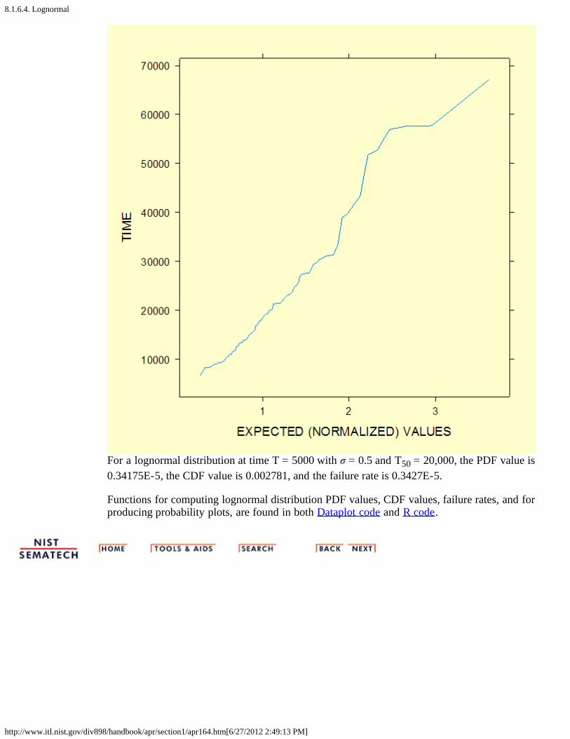
Lognormalprobabilityplot
We generated 100 random numbers from a lognormal distribution with shape 0.5 and medianlife 20,000. To see how well these random lognormal data points are fit by a lognormaldistribution, we generate the lognormal probability plot shown below. Points that line upapproximately on a straight line indicates a good fit to a lognormal (with shape 0.5). The timethat corresponds to the (normalized) x-axis T50 of 1 is the estimated T50 according to the data.In this case it is close to 20,000, as expected.
8.1.6.4. Lognormal
http://www.itl.nist.gov/div898/handbook/apr/section1/apr164.htm[6/27/2012 2:49:13 PM]
For a lognormal distribution at time T = 5000 with σ = 0.5 and T50 = 20,000, the PDF value is0.34175E-5, the CDF value is 0.002781, and the failure rate is 0.3427E-5.
Functions for computing lognormal distribution PDF values, CDF values, failure rates, and forproducing probability plots, are found in both Dataplot code and R code.

8.1.6.5. Gamma
http://www.itl.nist.gov/div898/handbook/apr/section1/apr165.htm[6/27/2012 2:49:15 PM]
8. Assessing Product Reliability 8.1. Introduction 8.1.6. What are the basic lifetime distribution models used for non-repairable populations?
8.1.6.5. Gamma
Formulasfor thegammamodel
Formulas and Plots
There are two ways of writing (parameterizing) the gamma distribution that are common inthe literature. In addition, different authors use different symbols for the shape and scaleparameters. Below we show two ways of writing the gamma, with "shape" parameter a = α,and "scale" parameter b = 1/β.
Theexponentialis a specialcase of thegamma
Note: When a = 1, the gamma reduces to an exponential distribution with b = λ.
Another well-known statistical distribution, the Chi-Square, is also a special case of thegamma. A Chi-Square distribution with n degrees of freedom is the same as a gamma with a= n/2 and b = 0.5 (or β = 2).
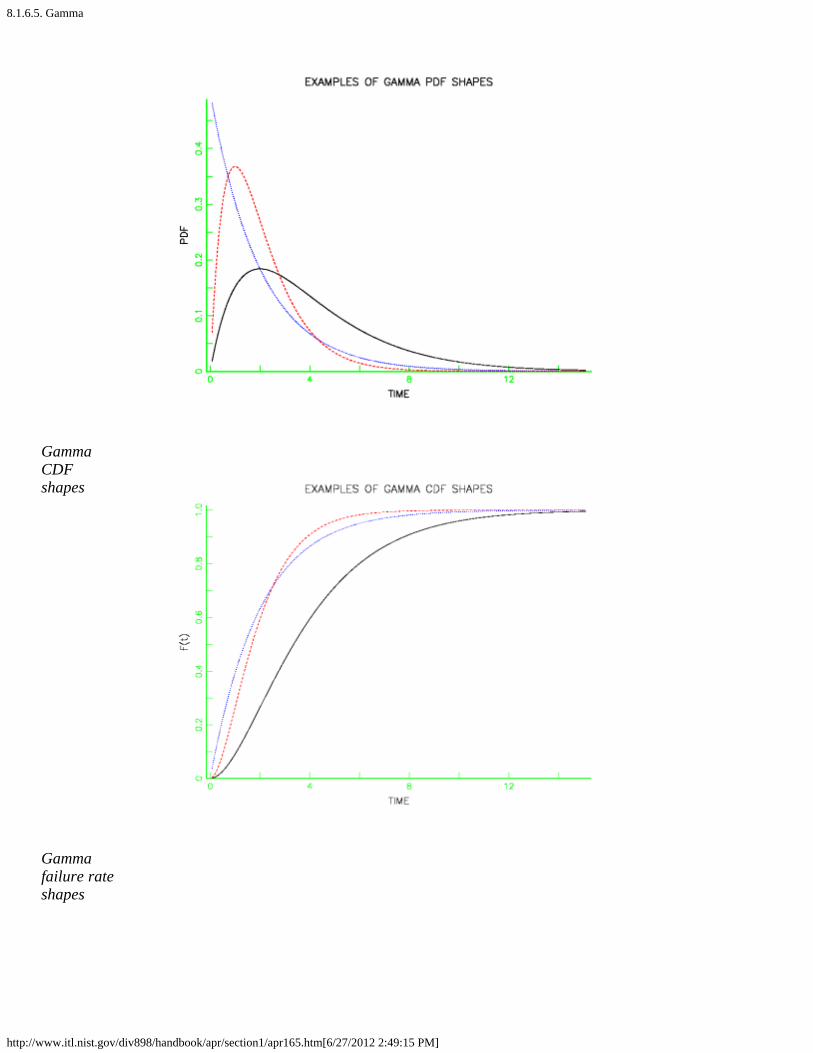
The following plots give examples of gamma PDF, CDF and failure rate shapes.
Shapes forgammadata
8.1.6.5. Gamma
http://www.itl.nist.gov/div898/handbook/apr/section1/apr165.htm[6/27/2012 2:49:15 PM]
GammaCDFshapes
Gammafailure rateshapes
8.1.6.5. Gamma
http://www.itl.nist.gov/div898/handbook/apr/section1/apr165.htm[6/27/2012 2:49:15 PM]
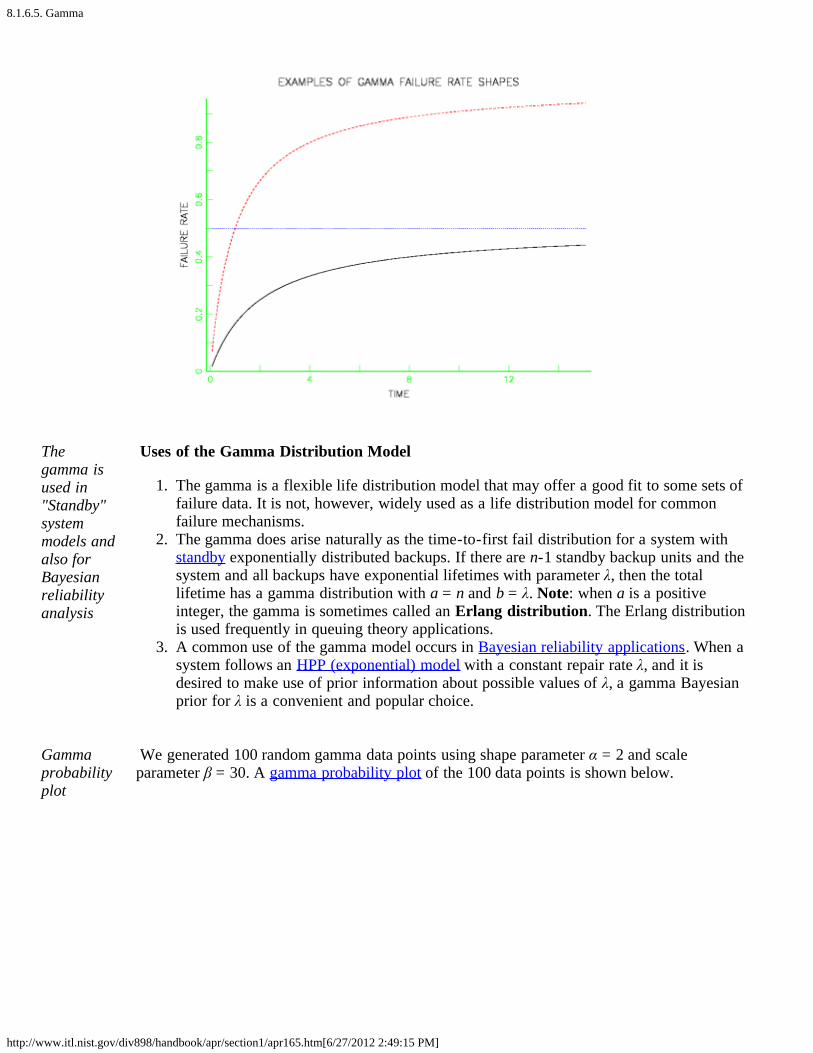
Thegamma isused in"Standby"systemmodels andalso forBayesianreliabilityanalysis
Uses of the Gamma Distribution Model
1. The gamma is a flexible life distribution model that may offer a good fit to some sets offailure data. It is not, however, widely used as a life distribution model for commonfailure mechanisms.
2. The gamma does arise naturally as the time-to-first fail distribution for a system withstandby exponentially distributed backups. If there are n-1 standby backup units and thesystem and all backups have exponential lifetimes with parameter λ, then the totallifetime has a gamma distribution with a = n and b = λ. Note: when a is a positiveinteger, the gamma is sometimes called an Erlang distribution. The Erlang distributionis used frequently in queuing theory applications.
3. A common use of the gamma model occurs in Bayesian reliability applications. When asystem follows an HPP (exponential) model with a constant repair rate λ, and it isdesired to make use of prior information about possible values of λ, a gamma Bayesianprior for λ is a convenient and popular choice.
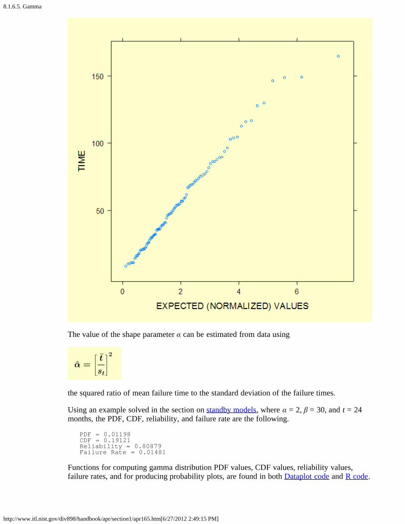
Gammaprobabilityplot
We generated 100 random gamma data points using shape parameter α = 2 and scaleparameter β = 30. A gamma probability plot of the 100 data points is shown below.
8.1.6.5. Gamma
http://www.itl.nist.gov/div898/handbook/apr/section1/apr165.htm[6/27/2012 2:49:15 PM]
The value of the shape parameter α can be estimated from data using
the squared ratio of mean failure time to the standard deviation of the failure times.
Using an example solved in the section on standby models, where α = 2, β = 30, and t = 24months, the PDF, CDF, reliability, and failure rate are the following.
PDF = 0.01198 CDF = 0.19121 Reliability = 0.80879 Failure Rate = 0.01481
Functions for computing gamma distribution PDF values, CDF values, reliability values,failure rates, and for producing probability plots, are found in both Dataplot code and R code.

8.1.6.5. Gamma
http://www.itl.nist.gov/div898/handbook/apr/section1/apr165.htm[6/27/2012 2:49:15 PM]

8.1.6.6. Fatigue life (Birnbaum-Saunders)
http://www.itl.nist.gov/div898/handbook/apr/section1/apr166.htm[6/27/2012 2:49:16 PM]
8. Assessing Product Reliability 8.1. Introduction 8.1.6. What are the basic lifetime distribution models used for non-repairable populations?
8.1.6.6. Fatigue life (Birnbaum-Saunders)
A modelbased oncycles ofstresscausingdegradationor crackgrowth
In 1969, Birnbaum and Saunders described a life distribution model that could be derivedfrom a physical fatigue process where crack growth causes failure. Since one of the best waysto choose a life distribution model is to derive it from a physical/statistical argument that isconsistent with the failure mechanism, the Birnbaum-Saunders fatigue life distribution isworth considering.
Formulasand shapesfor thefatigue lifemodel
Formulas and Plots for the Birnbaum-Saunders Model
The PDF, CDF, mean and variance for the Birnbaum-Saunders distribution are shown below.The parameters are: γ, a shape parameter; and μ, a scale parameter. These are the parameterswe will use in our discussion, but there are other choices also common in the literature (see theparameters used for the derivation of the model).
PDF shapes for the model vary from highly skewed and long tailed (small gamma values) tonearly symmetric and short tailed as gamma increases. This is shown in the figure below.

8.1.6.6. Fatigue life (Birnbaum-Saunders)
http://www.itl.nist.gov/div898/handbook/apr/section1/apr166.htm[6/27/2012 2:49:16 PM]
Corresponding failure rate curves are shown in the next figure.
If crackgrowth ineach stresscycle is arandom
Derivation and Use of the Birnbaum-Saunders Model:
Consider a material that continually undergoes cycles of stress loads. During each cycle, adominant crack grows towards a critical length that will cause failure. Under repeatedapplication of n cycles of loads, the total extension of the dominant crack can be written as

8.1.6.6. Fatigue life (Birnbaum-Saunders)
http://www.itl.nist.gov/div898/handbook/apr/section1/apr166.htm[6/27/2012 2:49:16 PM]
amountindependentof pastcycles ofgrowth, theFatigue Lifemode modelmay apply.
and we assume the Yj are independent and identically distributed non-negative randomvariables with mean μ and variance σ2. Suppose failure occurs at the N-th cycle, when Wnfirst exceeds a constant critical value w. If n is large, we can use a central limit theoremargument to conclude that
Since there are many cycles, each lasting a very short time, we can replace the discretenumber of cycles N needed to reach failure by the continuous time tf needed to reach failure.The CDF F(t) of tf is given by
Here Φ denotes the standard normal CDF. Writing the model with parameters α and β is analternative way of writing the Birnbaum-Saunders distribution that is often used (α = γ and β= μ, as compared to the way the formulas were parameterized earlier in this section).
Note: The critical assumption in the derivation, from a physical point of view, is that the crackgrowth during any one cycle is independent of the growth during any other cycle. Also, thegrowth has approximately the same random distribution, from cycle to cycle. This is a verydifferent situation from the proportional degradation argument used to derive a log normaldistribution model, with the rate of degradation at any point in time depending on the totalamount of degradation that has occurred up to that time.
This kind ofphysicaldegradationis consistentwithMiner'sRule.
The Birnbaum-Saunders assumption, while physically restrictive, is consistent with adeterministic model from materials physics known as Miner's Rule (Miner's Rule implies thatthe damage that occurs after n cycles, at a stress level that produces a fatigue life of N cycles,is proportional to n/N). So, when the physics of failure suggests Miner's Rule applies, theBirnbaum-Saunders model is a reasonable choice for a life distribution model.
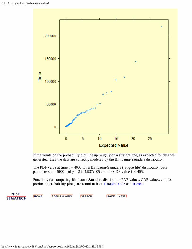
Birnbaum-Saundersprobabilityplot
We generated 100 random numbers from a Birnbaum-Saunders distribution where μ = 5000and γ = 2, and created a fatigue life probability plot of the 100 data points.
8.1.6.6. Fatigue life (Birnbaum-Saunders)
http://www.itl.nist.gov/div898/handbook/apr/section1/apr166.htm[6/27/2012 2:49:16 PM]
If the points on the probability plot line up roughly on a straight line, as expected for data wegenerated, then the data are correctly modeled by the Birnbaum-Saunders distribution.
The PDF value at time t = 4000 for a Birnbaum-Saunders (fatigue life) distribution withparameters μ = 5000 and γ = 2 is 4.987e-05 and the CDF value is 0.455.
Functions for computing Birnbaum-Saunders distribution PDF values, CDF values, and forproducing probability plots, are found in both Dataplot code and R code.

8.1.6.7. Proportional hazards model
http://www.itl.nist.gov/div898/handbook/apr/section1/apr167.htm[6/27/2012 2:49:17 PM]
8. Assessing Product Reliability 8.1. Introduction 8.1.6. What are the basic lifetime distribution models used for non-repairable populations?
8.1.6.7. Proportional hazards model
Theproportionalhazardsmodel isoften usedin survivalanalysis(medicaltesting)studies. It isnot usedmuch withengineeringdata
The proportional hazards model, proposed by Cox (1972),has been used primarily in medical testing analysis, to modelthe effect of secondary variables on survival. It is more likean acceleration model than a specific life distribution model,and its strength lies in its ability to model and test manyinferences about survival without making any specificassumptions about the form of the life distribution model.
This section will give only a brief description of theproportional hazards model, since it has limited engineeringapplications.
Proportional Hazards Model Assumption
Let z = {x, y, ...} be a vector of 1 or more explanatoryvariables believed to affect lifetime. These variables may becontinuous (like temperature in engineering studies, ordosage level of a particular drug in medical studies) or theymay be indicator variables with the value 1 if a given factoror condition is present, and 0 otherwise.
Let the hazard rate for a nominal (or baseline) set z0 =(x0,y0, ...) of these variables be given by h0(t), with h0(t)denoting legitimate hazard function (failure rate) for someunspecified life distribution model.
Theproportionalhazardmodelassumeschanging astressvariable (orexplanatoryvariable)has theeffect ofmultiplyingthe hazardrate by aconstant.
The proportional hazards model assumes we can write thechanged hazard function for a new value of z as
hz(t) = g(z)h0(t)
In other words, changing z, the explanatory variable vector,results in a new hazard function that is proportional to thenominal hazard function, and the proportionality constant isa function of z, g(z), independent of the time variable t.
A common and useful form for f(z) is the Log Linear Modelwhich has the equation: g(x) = eax for one variable, g(x,y) =eax+by for two variables, etc.
Properties and Applications of the Proportional Hazards

8.1.6.7. Proportional hazards model
http://www.itl.nist.gov/div898/handbook/apr/section1/apr167.htm[6/27/2012 2:49:17 PM]
Model
1. The proportional hazards model is equivalent to theacceleration factor concept if and only if the lifedistribution model is a Weibull (which includes theexponential model, as a special case). For a Weibullwith shape parameter , and an acceleration factor AFbetween nominal use fail time t0 and high stress failtime ts (with t0 = AFts) we have g(s) = AF . In otherwords, hs(t) = AF h0(t).
2. Under a log-linear model assumption for g(z), withoutany further assumptions about the life distributionmodel, it is possible to analyze experimental data andcompute maximum likelihood estimates and uselikelihood ratio tests to determine which explanatoryvariables are highly significant. In order to do this kindof analysis, however, special software is needed.
More details on the theory and applications of theproportional hazards model may be found in Cox and Oakes(1984).

8.1.7. What are some basic repair rate models used for repairable systems?
http://www.itl.nist.gov/div898/handbook/apr/section1/apr17.htm[6/27/2012 2:49:18 PM]
8. Assessing Product Reliability 8.1. Introduction
8.1.7. What are some basic repair rate modelsused for repairable systems?
Models forrepairrates ofrepairablesystems
N(t), M(t) and m(t) were defined in the section on RepairRates. Repair rate models are defined by first picking afunctional form for M(t), the expected number of cumulativefailures by time t. Taking the derivative of this gives the repairrate model m(t).
In the next three sections we will describe three models, ofincreasing complexity, for M(t). They are: the HomogeneousPoisson Process, the Non-Homogeneous Poisson Processfollowing a Power law, and the Non-Homogeneous PoissonProcess following an Exponential law.
8.1.7.1. Homogeneous Poisson Process (HPP)
http://www.itl.nist.gov/div898/handbook/apr/section1/apr171.htm[6/27/2012 2:49:18 PM]
8. Assessing Product Reliability 8.1. Introduction 8.1.7. What are some basic repair rate models used for repairable systems?
8.1.7.1. Homogeneous Poisson Process (HPP)
Repair rate(ROCOF)models andformulas
The simplest useful model for M(t) is M(t) = λ t and the repair rate (or ROCOF) is theconstant m(t) = λ. This model comes about when the interarrival times between failuresare independent and identically distributed according to the exponential distribution,with parameter λ. This basic model is also known as a Homogeneous Poisson Process(HPP). The following formulas apply:
HPP modelfits flatportion of"bathtub"curve
Despite the simplicity of this model, it is widely used for repairable equipment andsystems throughout industry. Justification for this comes, in part, from the shape of theempirical Bathtub Curve. Most systems (or complex tools or equipment) spend most oftheir "lifetimes" operating in the long flat constant repair rate portion of the BathtubCurve. The HPP is the only model that applies to that portion of the curve, so it is themost popular model for system reliability evaluation and reliability test planning.
Planning reliability assessment tests (under the HPP assumption) is covered in a latersection, as is estimating the MTBF from system failure data and calculating upper andlower confidence limits.
Poissonrelationship
In the HPP model, the probability of having exactly k failures by time T is given by thePoisson distribution with mean λ T (see formula for P{N(T) = k} above).

8.1.7.2. Non-Homogeneous Poisson Process (NHPP) - power law
http://www.itl.nist.gov/div898/handbook/apr/section1/apr172.htm[6/27/2012 2:49:19 PM]
8. Assessing Product Reliability 8.1. Introduction 8.1.7. What are some basic repair rate models used for repairable systems?
8.1.7.2. Non-Homogeneous Poisson Process(NHPP) - power law
The repairrate for aNHPPfollowing thePower law
A flexible model (that has been very successful in manyapplications) for the expected number of failures in the first thours, M(t), is given by the polynomial
The repair rate (or ROCOF) for this model is
The Powerlaw model isvery flexibleand containsthe HPP(exponential)model as aspecial case
The HPP model has a the constant repair rate m(t) = . Ifwe substitute an arbitrary function (t) for , we have aNon Homogeneous Poisson Process (NHPP) with IntensityFunction . If
then we have an NHPP with a Power Law intensityfunction (the "intensity function" is another name for therepair rate m(t)).
Because of the polynomial nature of the ROCOF, this modelis very flexible and can model both increasing (b>1 or <0) and decreasing (0 < b < 1 or 0 < < 1)) failure rates.When b = 1 or = 0, the model reduces to the HPPconstant repair rate model.
Probabilitiesof failure forall NHPPprocessescan easily becalculatedbased on thePoissonformula
Probabilities of a given number of failures for the NHPPmodel are calculated by a straightforward generalization ofthe formulas for the HPP. Thus, for any NHPP
and for the Power Law model:

8.1.7.2. Non-Homogeneous Poisson Process (NHPP) - power law
http://www.itl.nist.gov/div898/handbook/apr/section1/apr172.htm[6/27/2012 2:49:19 PM]
The PowerLaw modelis also calledthe DuaneModel andthe AMSAAmodel
Other names for the Power Law model are: the DuaneModel and the AMSAA model. AMSAA stands for theUnited States Army Materials System Analysis Activity,where much theoretical work describing the Power Lawmodel was performed in the 1970's.
It is alsocalled aWeibullProcess - butthis name ismisleadingand shouldbe avoided
The time to the first fail for a Power Law process has aWeibull distribution with shape parameter b andcharacteristic life a. For this reason, the Power Law model issometimes called a Weibull Process. This name is confusingand should be avoided, however, since it mixes a lifedistribution model applicable to the lifetimes of a non-repairable population with a model for the inter-arrivaltimes of failures of a repairable population.
For any NHPP process with intensity function m(t), thedistribution function (CDF) for the inter-arrival time tothe next failure, given a failure just occurred at time T, isgiven by
Once afailureoccurs, thewaiting timeto the nextfailure for anNHPP has asimple CDFformula
In particular, for the Power Law the waiting time to the nextfailure, given a failure at time T, has distribution function
This inter arrival time CDF can be used to derive a simplealgorithm for simulating NHPP Power Law Data.

8.1.7.3. Exponential law
http://www.itl.nist.gov/div898/handbook/apr/section1/apr173.htm[6/27/2012 2:49:20 PM]
8. Assessing Product Reliability 8.1. Introduction 8.1.7. What are some basic repair rate models used for repairable systems?
8.1.7.3. Exponential law
TheExponentialLaw isanotherflexibleNHPPmodel
An NHPP with ROCOF or intensity function given by
is said to follow an Exponential Law. This is also called thelog-linear model or the Cox-Lewis model.
A system whose repair rate follows this flexible model isimproving if < 0 and deteriorating if >0. When = 0,the Exponential Law reduces to the HPP constant repair ratemodel

8.1.8. How can you evaluate reliability from the "bottom-up" (component failure mode to system failure rate)?
http://www.itl.nist.gov/div898/handbook/apr/section1/apr18.htm[6/27/2012 2:49:21 PM]
8. Assessing Product Reliability 8.1. Introduction
8.1.8. How can you evaluate reliability from the"bottom-up" (component failure mode tosystem failure rate)?
Severalsimplemodels canbe used tocalculatesystemfailurerates,startingwith failurerates forfailuremodeswithinindividualsystemcomponents
This section deals with models and methods that apply tonon-repairable components and systems. Models for failurerates (and not repair rates) are described. The next sectioncovers models for (repairable) system reliability growth.
We use the Competing Risk Model to go from componentfailure modes to component failure rates. Next we use theSeries Model to go from components to assemblies andsystems. These models assume independence and "firstfailure mode to reach failure causes both the component andthe system to fail".
If some components are "in parallel", so that the system cansurvive one (or possibly more) component failures, we havethe parallel or redundant model. If an assembly has n identicalcomponents, at least r of which must be working for thesystem to work, we have what is known as the r out of nmodel.
The standby model uses redundancy like the parallel model,except that the redundant unit is in an off-state (not exercised)until called upon to replace a failed unit.
This section describes these various models. The lastsubsection shows how complex systems can be evaluatedusing the various models as building blocks.
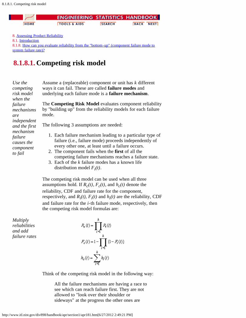
8.1.8.1. Competing risk model
http://www.itl.nist.gov/div898/handbook/apr/section1/apr181.htm[6/27/2012 2:49:21 PM]
8. Assessing Product Reliability 8.1. Introduction 8.1.8. How can you evaluate reliability from the "bottom-up" (component failure mode tosystem failure rate)?
8.1.8.1. Competing risk model
Use thecompetingrisk modelwhen thefailuremechanismsareindependentand the firstmechanismfailurecauses thecomponentto fail
Assume a (replaceable) component or unit has k differentways it can fail. These are called failure modes andunderlying each failure mode is a failure mechanism.
The Competing Risk Model evaluates component reliabilityby "building up" from the reliability models for each failuremode.
The following 3 assumptions are needed:
1. Each failure mechanism leading to a particular type offailure (i.e., failure mode) proceeds independently ofevery other one, at least until a failure occurs.
2. The component fails when the first of all thecompeting failure mechanisms reaches a failure state.
3. Each of the k failure modes has a known lifedistribution model Fi(t).
The competing risk model can be used when all threeassumptions hold. If Rc(t), Fc(t), and hc(t) denote thereliability, CDF and failure rate for the component,respectively, and Ri(t), Fi(t) and hi(t) are the reliability, CDFand failure rate for the i-th failure mode, respectively, thenthe competing risk model formulas are:
Multiplyreliabilitiesand addfailure rates
Think of the competing risk model in the following way:
All the failure mechanisms are having a race tosee which can reach failure first. They are notallowed to "look over their shoulder orsideways" at the progress the other ones are

8.1.8.1. Competing risk model
http://www.itl.nist.gov/div898/handbook/apr/section1/apr181.htm[6/27/2012 2:49:21 PM]
making. They just go their own way as fast asthey can and the first to reach "failure" causesthe component to fail.
Under these conditions the component reliabilityis the product of the failure mode reliabilities andthe component failure rate is just the sum of thefailure mode failure rates.
Note that the above holds for any arbitrary life distributionmodel, as long as "independence" and "first mechanismfailure causes the component to fail" holds.
When we learn how to plot and analyze reliability data inlater sections, the methods will be applied separately to eachfailure mode within the data set (considering failures due toall other modes as "censored run times"). With this approach,the competing risk model provides the glue to put the piecesback together again.
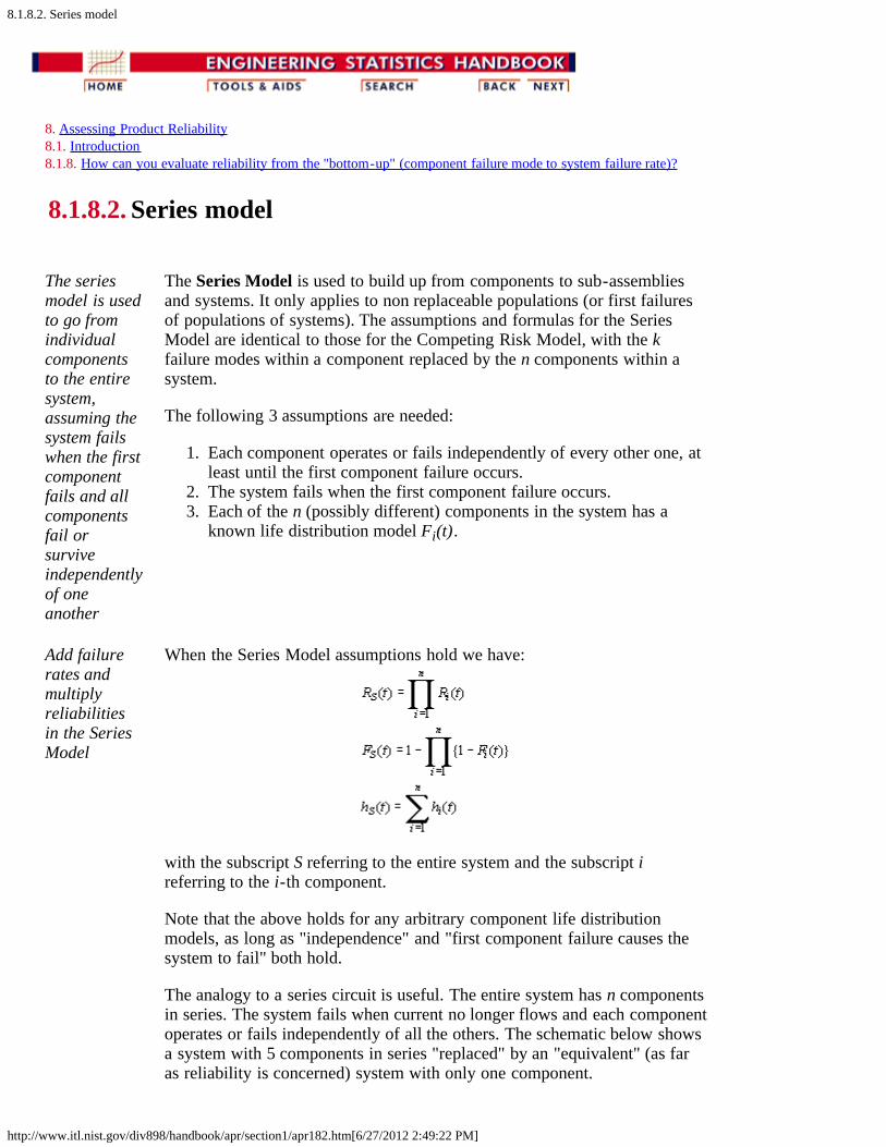
8.1.8.2. Series model
http://www.itl.nist.gov/div898/handbook/apr/section1/apr182.htm[6/27/2012 2:49:22 PM]
8. Assessing Product Reliability 8.1. Introduction 8.1.8. How can you evaluate reliability from the "bottom-up" (component failure mode to system failure rate)?
8.1.8.2. Series model
The seriesmodel is usedto go fromindividualcomponentsto the entiresystem,assuming thesystem failswhen the firstcomponentfails and allcomponentsfail orsurviveindependentlyof oneanother
The Series Model is used to build up from components to sub-assembliesand systems. It only applies to non replaceable populations (or first failuresof populations of systems). The assumptions and formulas for the SeriesModel are identical to those for the Competing Risk Model, with the kfailure modes within a component replaced by the n components within asystem.
The following 3 assumptions are needed:
1. Each component operates or fails independently of every other one, atleast until the first component failure occurs.
2. The system fails when the first component failure occurs. 3. Each of the n (possibly different) components in the system has a
known life distribution model Fi(t).
Add failurerates andmultiplyreliabilitiesin the SeriesModel
When the Series Model assumptions hold we have:
with the subscript S referring to the entire system and the subscript ireferring to the i-th component.
Note that the above holds for any arbitrary component life distributionmodels, as long as "independence" and "first component failure causes thesystem to fail" both hold.
The analogy to a series circuit is useful. The entire system has n componentsin series. The system fails when current no longer flows and each componentoperates or fails independently of all the others. The schematic below showsa system with 5 components in series "replaced" by an "equivalent" (as faras reliability is concerned) system with only one component.
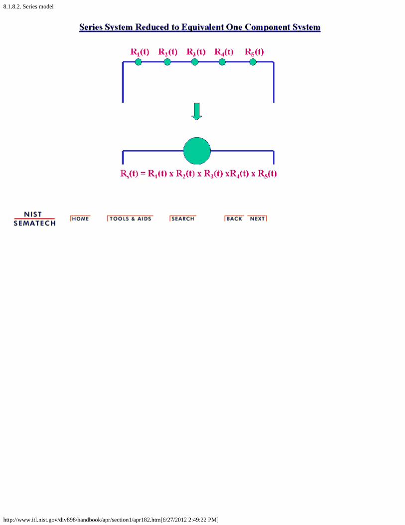
8.1.8.2. Series model
http://www.itl.nist.gov/div898/handbook/apr/section1/apr182.htm[6/27/2012 2:49:22 PM]

8.1.8.3. Parallel or redundant model
http://www.itl.nist.gov/div898/handbook/apr/section1/apr183.htm[6/27/2012 2:49:23 PM]
8. Assessing Product Reliability 8.1. Introduction 8.1.8. How can you evaluate reliability from the "bottom-up" (component failure mode to system failure rate)?
8.1.8.3. Parallel or redundant model
The parallelmodelassumes all ncomponentsthat make upa systemoperateindependentlyand thesystem worksas long as atleast onecomponentstill works
The opposite of a series model, for which the first component failure causesthe system to fail, is a parallel model for which all the components have tofail before the system fails. If there are n components, any (n-1) of themmay be considered redundant to the remaining one (even if the componentsare all different). When the system is turned on, all the components operateuntil they fail. The system reaches failure at the time of the last componentfailure.
The assumptions for a parallel model are:
1. All components operate independently of one another, as far asreliability is concerned.
2. The system operates as long as at least one component is stilloperating. System failure occurs at the time of the last componentfailure.
3. The CDF for each component is known.
MultiplycomponentCDF's to getthe systemCDF for aparallelmodel
For a parallel model, the CDF Fs(t) for the system is just the product of theCDF's Fi(t) for the components or
Rs(t) and hs(t) can be evaluated using basic definitions, once we have Fs(t).
The schematic below represents a parallel system with 5 components and the(reliability) equivalent 1 component system with a CDF Fs equal to theproduct of the 5 component CDF's.
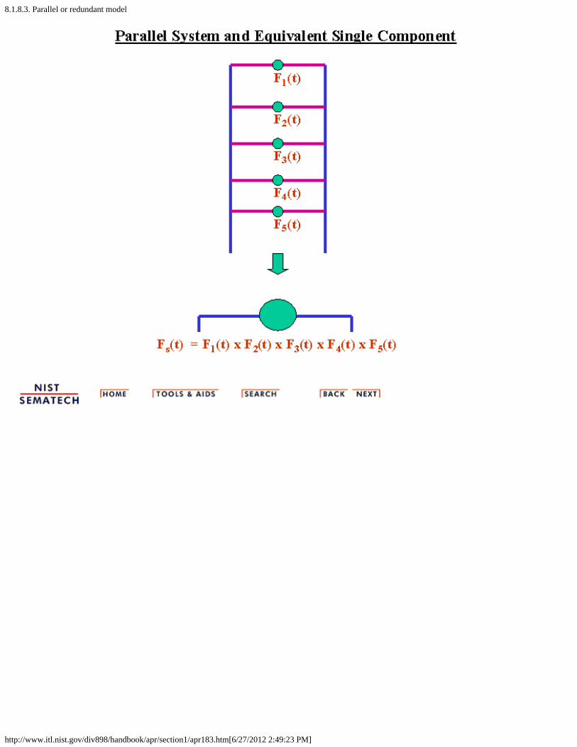
8.1.8.3. Parallel or redundant model
http://www.itl.nist.gov/div898/handbook/apr/section1/apr183.htm[6/27/2012 2:49:23 PM]

8.1.8.4. R out of N model
http://www.itl.nist.gov/div898/handbook/apr/section1/apr184.htm[6/27/2012 2:49:24 PM]
8. Assessing Product Reliability 8.1. Introduction 8.1.8. How can you evaluate reliability from the "bottom-up" (component failure mode tosystem failure rate)?
8.1.8.4. R out of N model
An r out ofn model isa systemthatsurviveswhen atleast r ofitscomponentsareworking(any r)
An "r out of n" system contains both the series system modeland the parallel system model as special cases. The systemhas n components that operate or fail independently of oneanother and as long as at least r of these components (any r)survive, the system survives. System failure occurs when the(n-r+1)th component failure occurs.
When r = n, the r out of n model reduces to the series model.When r = 1, the r out of n model becomes the parallel model.
We treat here the simple case where all the components areidentical.
Formulas and assumptions for r out of n model (identicalcomponents):
1. All components have the identical reliability functionR(t).
2. All components operate independently of one another(as far as failure is concerned).
3. The system can survive any (n-r) of the componentsfailing. The system fails at the instant of the (n-r+1)thcomponent failure.
Formulafor an r outof n systemwhere thecomponentsareidentical
System reliability is given by adding the probability ofexactly r components surviving to time t to the probability ofexactly (r+1) components surviving, and so on up to theprobability of all components surviving to time t. These arebinomial probabilities (with p = R(t)), so the systemreliability is given by:
Note: If we relax the assumption that all the components areidentical, then Rs(t) would be the sum of probabilitiesevaluated for all possible terms that could be formed bypicking at least r survivors and the corresponding failures.The probability for each term is evaluated as a product ofR(t)'s and F(t)'s. For example, for n = 4 and r = 2, the system

8.1.8.4. R out of N model
http://www.itl.nist.gov/div898/handbook/apr/section1/apr184.htm[6/27/2012 2:49:24 PM]
reliability would be (abbreviating the notation for R(t) andF(t) by using only R and F)
Rs = R1R2F3F4 + R1R3F2F4 + R1R4F2F3 + R2R3F1F4 + R2R4F1F3 + R3R4F1F2 + R1R2R3F4 + R1R3R4F2 + R1R2R4F3 + R2R3R4F1 + R1R2R3R4
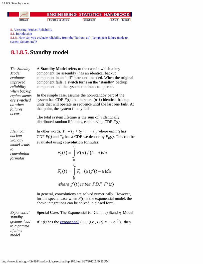
8.1.8.5. Standby model
http://www.itl.nist.gov/div898/handbook/apr/section1/apr185.htm[6/27/2012 2:49:25 PM]
8. Assessing Product Reliability 8.1. Introduction 8.1.8. How can you evaluate reliability from the "bottom-up" (component failure mode tosystem failure rate)?
8.1.8.5. Standby model
The StandbyModelevaluatesimprovedreliabilitywhen backupreplacementsare switchedon whenfailuresoccur.
A Standby Model refers to the case in which a keycomponent (or assembly) has an identical backupcomponent in an "off" state until needed. When the originalcomponent fails, a switch turns on the "standby" backupcomponent and the system continues to operate.
In the simple case, assume the non-standby part of thesystem has CDF F(t) and there are (n-1) identical backupunits that will operate in sequence until the last one fails. Atthat point, the system finally fails.
The total system lifetime is the sum of n identicallydistributed random lifetimes, each having CDF F(t).
IdenticalbackupStandbymodel leadstoconvolutionformulas
In other words, Tn = t1 + t2+ ... + tn, where each ti hasCDF F(t) and Tn has a CDF we denote by Fn(t). This can beevaluated using convolution formulas:
In general, convolutions are solved numerically. However,for the special case when F(t) is the exponential model, theabove integrations can be solved in closed form.
Exponentialstandbysystems leadto a gammalifetimemodel
Special Case: The Exponential (or Gamma) Standby Model
If F(t) has the exponential CDF (i.e., F(t) = 1 - e-lt ), then

8.1.8.5. Standby model
http://www.itl.nist.gov/div898/handbook/apr/section1/apr185.htm[6/27/2012 2:49:25 PM]
and the PDF fn(t) is the well-known gamma distribution.
Example: An unmanned space probe sent out to explore thesolar system has an onboard computer with reliabilitycharacterized by the exponential distribution with a MeanTime To Failure (MTTF) of 1/ = 30 months (a constantfailure rate of 1/30 = .033 fails per month). The probabilityof surviving a two year mission is only e-24/30 = .45. If,however, a second computer is included in the probe in astandby mode, the reliability at 24 months (using the aboveformula for F2) becomes .8 × .449 + .449 = .81. The failurerate at 24 months (f2/[1-F2]) reduces to [(24/900)×.449]/.81 = .015 fails per month. At 12 months the failurerate is only .0095 fails per month, which is less than 1/3 ofthe failure rate calculated for the non-standby case.
Standby units (as the example shows) are an effective wayof increasing reliability and reducing failure rates, especiallyduring the early stages of product life. Their improvementeffect is similar to, but greater than, that of parallelredundancy . The drawback, from a practical standpoint, isthe expense of extra components that are not needed forfunctionality.
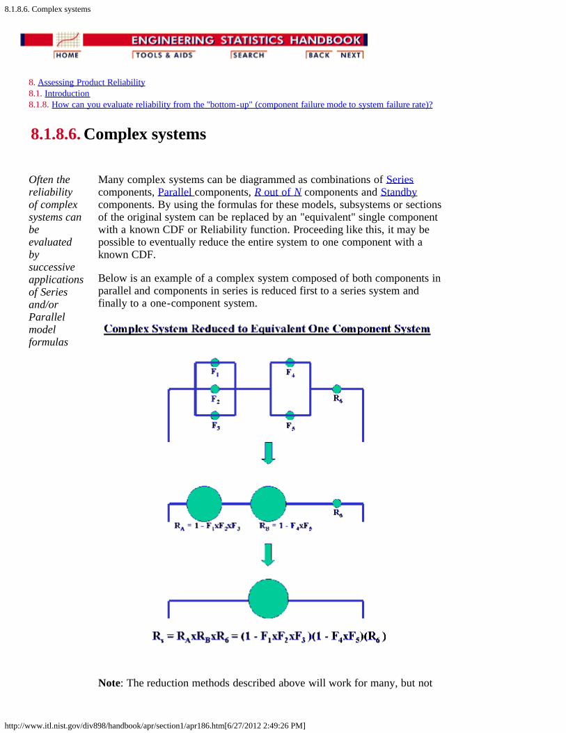
8.1.8.6. Complex systems
http://www.itl.nist.gov/div898/handbook/apr/section1/apr186.htm[6/27/2012 2:49:26 PM]
8. Assessing Product Reliability 8.1. Introduction 8.1.8. How can you evaluate reliability from the "bottom-up" (component failure mode to system failure rate)?
8.1.8.6. Complex systems
Often thereliabilityof complexsystems canbeevaluatedbysuccessiveapplicationsof Seriesand/orParallelmodelformulas
Many complex systems can be diagrammed as combinations of Seriescomponents, Parallel components, R out of N components and Standbycomponents. By using the formulas for these models, subsystems or sectionsof the original system can be replaced by an "equivalent" single componentwith a known CDF or Reliability function. Proceeding like this, it may bepossible to eventually reduce the entire system to one component with aknown CDF.
Below is an example of a complex system composed of both components inparallel and components in series is reduced first to a series system andfinally to a one-component system.
Note: The reduction methods described above will work for many, but not

8.1.8.6. Complex systems
http://www.itl.nist.gov/div898/handbook/apr/section1/apr186.htm[6/27/2012 2:49:26 PM]
all, systems. Some systems with a complicated operational logic structurewill need a more formal structural analysis methodology. This methodologydeals with subjects such as event trees, Boolean representations, coherentstructures, cut sets and decompositions, and is beyond the present scope ofthis Handbook.

8.1.9. How can you model reliability growth?
http://www.itl.nist.gov/div898/handbook/apr/section1/apr19.htm[6/27/2012 2:49:26 PM]
8. Assessing Product Reliability 8.1. Introduction
8.1.9. How can you model reliability growth?
A reliabilityimprovementtest is aformalprocedureaimed atdiscoveringand fixingsystemreliabilityflaws
During the early stages of developing and prototypingcomplex systems, reliability often does not meet customerrequirements. A formal test procedure aimed at discoveringand fixing causes of unreliability is known as a ReliabilityImprovement Test. This test focuses on system design,system assembly and component selection weaknesses thatcause failures.
A typical reliability improvement test procedure would be torun a prototype system, as the customer might for a periodof several weeks, while a multidisciplined team of engineersand technicians (design, quality, reliability, manufacturing,etc.) analyze every failure that occurs. This team comes upwith root causes for the failures and develops design and/orassembly improvements to hopefully eliminate or reduce thefuture occurrence of that type of failure. As the testingcontinues, the improvements the team comes up with areincorporated into the prototype, so it is expected thatreliability will improve during the course of the test.
Repair ratesshould showanimprovementtrend duringthe course ofa reliabilityimprovementtest and thiscan bemodeledusing aNHPPmodel
Another name for reliability improvement testing is TAAFtesting, standing for Test, Analyze And Fix.
While only one model applies when a repairable system hasno improvement or degradation trends (the constant repairrate HPP model), there are infinitely many models that couldbe used to describe a system with a decreasing repair rate(reliability growth models).
Fortunately, one or two relatively simple models have beenvery successful in a wide range of industrial applications.Two models that have previously been described will beused in this section. These models are the NHPP Power LawModel and the NHPP Exponential Law Model. The PowerLaw Model underlies the frequently used graphicaltechnique known as Duane Plotting.

8.1.9.1. NHPP power law
http://www.itl.nist.gov/div898/handbook/apr/section1/apr191.htm[6/27/2012 2:49:27 PM]
8. Assessing Product Reliability 8.1. Introduction 8.1.9. How can you model reliability growth?
8.1.9.1. NHPP power law
If the PowerLaw applies,Repair Ratesimproveover timeaccording tothe formula
. Theexponent lies between0 and 1 andis called thereliabilitygrowth slope
This repairable system model was described in Section 8.1.7.2.The expected number of failures by time t has the form M(t) =atb and the repair rate has the form m(t) = abtb-1. This willmodel improvement when 0 < b < 1, with larger improvementscoming when b is smaller. As we will see in the next section onDuane Plotting, it is convenient to define = 1 - b and = ab, and write the repair rate as
m(t) =
Again we have improvement when 0 < < 1, with largerimprovement coming from larger values of . is known asthe Duane Plot slope or the reliability improvement GrowthSlope.
In terms of the original parameters for M(t), we have
Use of the Power Law model for reliability growth test datagenerally assumes the following:
1. While the test is ongoing, system improvements areintroduced that produce continual improvements in the rate ofsystem repair.
2. Over a long enough period of time the effect of theseimprovements can be modeled adequately by the continuouspolynomial repair rate improvement model .
When animprovementtest ends,the MTBFstaysconstant atits lastachievedvalue
3. When the improvement test ends at test time T and nofurther improvement actions are ongoing, the repair rate hasbeen reduced to . The repair rate remains constant fromthen on at this new (improved) level.
Assumption 3 means that when the test ends, the HPP constantrepair rate model takes over and the MTBF for the system fromthen on is the reciprocal of the final repair rate or . Ifwe estimate the expected number of failures up to time T by the
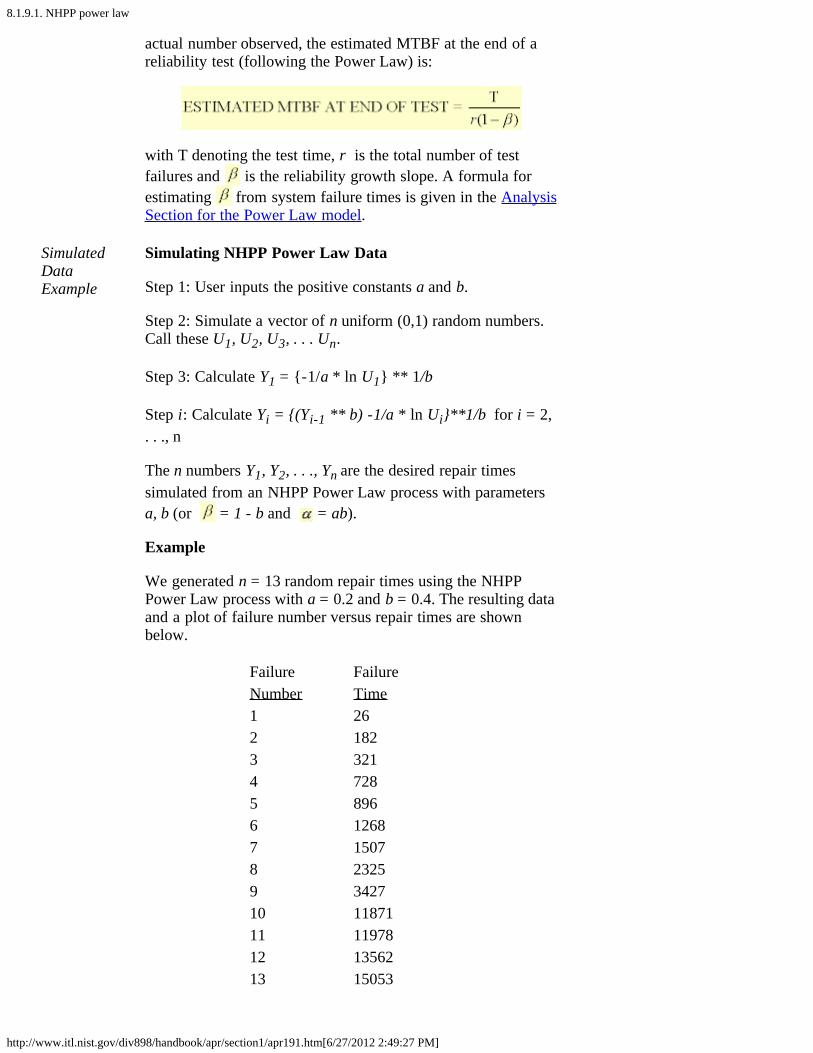
8.1.9.1. NHPP power law
http://www.itl.nist.gov/div898/handbook/apr/section1/apr191.htm[6/27/2012 2:49:27 PM]
actual number observed, the estimated MTBF at the end of areliability test (following the Power Law) is:
with T denoting the test time, r is the total number of testfailures and is the reliability growth slope. A formula forestimating from system failure times is given in the AnalysisSection for the Power Law model.
SimulatedDataExample
Simulating NHPP Power Law Data
Step 1: User inputs the positive constants a and b.
Step 2: Simulate a vector of n uniform (0,1) random numbers.Call these U1, U2, U3, . . . Un.
Step 3: Calculate Y1 = {-1/a * ln U1} ** 1/b
Step i: Calculate Yi = {(Yi-1 ** b) -1/a * ln Ui}**1/b for i = 2,. . ., n
The n numbers Y1, Y2, . . ., Yn are the desired repair timessimulated from an NHPP Power Law process with parametersa, b (or = 1 - b and = ab).
Example
We generated n = 13 random repair times using the NHPPPower Law process with a = 0.2 and b = 0.4. The resulting dataand a plot of failure number versus repair times are shownbelow.
Failure FailureNumber Time1 262 1823 3214 7285 8966 12687 15078 23259 342710 1187111 1197812 1356213 15053
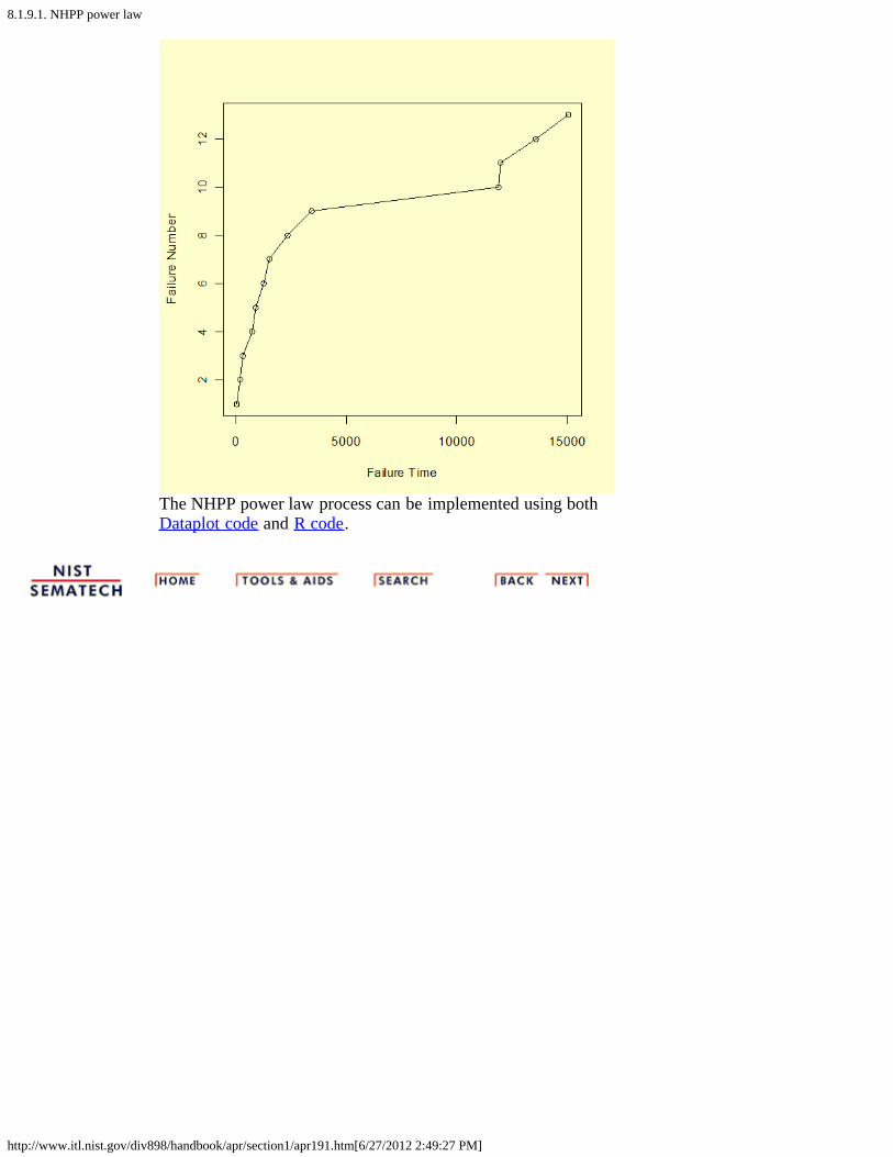
8.1.9.1. NHPP power law
http://www.itl.nist.gov/div898/handbook/apr/section1/apr191.htm[6/27/2012 2:49:27 PM]
The NHPP power law process can be implemented using bothDataplot code and R code.

8.1.9.2. Duane plots
http://www.itl.nist.gov/div898/handbook/apr/section1/apr192.htm[6/27/2012 2:49:28 PM]
8. Assessing Product Reliability 8.1. Introduction 8.1.9. How can you model reliability growth?
8.1.9.2. Duane plots
A plot on log-log paper ofsuccessiveMTBFestimatesversus systemtime of failfor reliabilityimprovementtest data iscalled aDuane Plot
The standard estimate of the MTBF for a system with a constant repair rate(an HPP system) is T/r, with T denoting the total time the system wasobserved and r is the total number of failures that occurred.
If we calculate successive MTBF estimates (called Cum MTBF Estimates),every time a failure occurs for a system undergoing reliability improvementtesting, we typically see a sequence of mostly increasing numbers.
In 1964, J. T. Duane observed that when he plotted these cum MTBFestimates versus the times of failure on log-log paper, the points tended toline up following a straight line. This was true for many different sets ofreliability improvement data and many other engineers have seen similarresults over the last three decades. This type of plot is called a Duane Plotand the slope of the best line through the points is called the reliabilitygrowth slope or Duane plot slope.
Points on aDuane plotline upapproximatelyon a straightline if thePower Lawmodel applies
Plotting a Duane Plot is simple. If the ith failure occurs at time ti, then plot tidivided by i (the "y"- axis value) versus the time ti (the "x"-axis value) onlog-log graph paper. Do this for all the test failures and draw the beststraight line you can following all these points.
Why does this "work"? Following the notation for repairable system models,we are plotting estimates of {t/M(t)} versus the time of failure t. If M(t)follows the Power Law (also described in the last section), then we areplotting estimates of t/atb versus the time of fail t. This is the same as
plotting versus t, with = 1-b . For a log-log scale plot, this willbe a straight line with slope and intercept (when t = 1) of - log10a.
In other words, a straight line on a Duane plot is equivalent to the NHPPPower Law Model with a reliability growth slope of = 1 - b and an "a"parameter equal to 10-intercept.
Note: A useful empirical rule of thumb based on Duane plots made frommany reliability improvement tests across many industries is the following:
Duane plotreliabilitygrowth slopesshould liebetween 0.3
The reliability improvement slope for virtually all reliabilityimprovement tests will be between 0.3 and 0.6. The lower end(0.3) describes a minimally effective test - perhaps the cross-functional team is inexperienced or the system has many failuremechanisms that are not well understood. The higher end (0.6)
8.1.9.2. Duane plots
http://www.itl.nist.gov/div898/handbook/apr/section1/apr192.htm[6/27/2012 2:49:28 PM]
and 0.6 approaches the empirical state of the art for reliabilityimprovement activities.
Examples ofDuane Plots
Duane Plot Example 1:
A reliability growth test lasted 1500 hours (approximately 10 weeks) andrecorded 8 failures at the following system hours: 33, 76, 145, 347, 555, 811,1212, 1499. After calculating successive cum MTBF estimates, a Duane plotshows these estimates versus system age on log vs log paper. The "best"straight line through the data points corresponds to a NHPP Power Lawmodel with reliability growth slope equal to the slope of the line. This lineis an estimate of the theoretical model line (assuming the Power Law holdsduring the course of the test) and the achieved MTBF at the end of the test isgiven by
T / [r (1- )]
with T denoting the total test time and r the number of failures. Results forthis particular reliability growth test follow. Failure # System Age of Failure Cum MTBF
1 33 332 76 383 145 48.34 347 86.85 555 111.06 811 135.27 1212 173.18 1499 187.3

8.1.9.2. Duane plots
http://www.itl.nist.gov/div898/handbook/apr/section1/apr192.htm[6/27/2012 2:49:28 PM]
The Duane plot indicates a reasonable fit to a Power Law NHPP model. Thereliability improvement slope (slope of line on Duane plot) is = 0.437(using the formula given in the section on reliability data analysis for thePower Law model) and the estimated MTBF achieved by the end of the1500 hour test is 1500/(8 × [1-0.437]) or 333 hours.
Duane Plot Example 2:
A Duane plot for the simulated Power Law data used in the Example in thepreceding section is shown below.
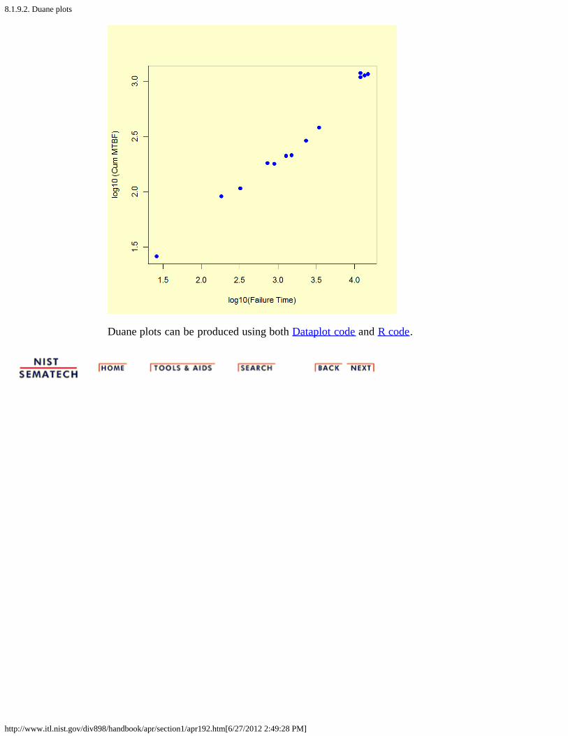
8.1.9.2. Duane plots
http://www.itl.nist.gov/div898/handbook/apr/section1/apr192.htm[6/27/2012 2:49:28 PM]
Duane plots can be produced using both Dataplot code and R code.
8.1.9.3. NHPP exponential law
http://www.itl.nist.gov/div898/handbook/apr/section1/apr193.htm[6/27/2012 2:49:29 PM]
8. Assessing Product Reliability 8.1. Introduction 8.1.9. How can you model reliability growth?
8.1.9.3. NHPP exponential law
TheExponentialLaw isanotherusefulreliabilitygrowthmodel totry whenthe Powerlaw is notfitting well
When the data points in a Duane plot show obviouscurvature, a model that might fit better is the NHPPExponential Law.
For this model, if < 0, the repair rate improves over timeaccording to
The corresponding cumulative expected failures model is
This approaches the maximum value of A expected failures ast goes to infinity, so the cumulative failures plot shouldclearly be bending over and asymptotically approaching avalue .
Rule of thumb: First try a Duane plot and the Power lawmodel. If that shows obvious lack of fit, try the ExponentialLaw model, estimating parameters using the formulas in theAnalysis Section for the Exponential law. A plot of cum failsversus time, along with the estimated M(t) curve, can be usedto judge goodness of fit.

8.1.10. How can Bayesian methodology be used for reliability evaluation?
http://www.itl.nist.gov/div898/handbook/apr/section1/apr1a.htm[6/27/2012 2:49:30 PM]
8. Assessing Product Reliability 8.1. Introduction
8.1.10. How can Bayesian methodology be used forreliability evaluation?
SeveralBayesianMethodsoverviewtopics arecovered inthis section
This section gives an overview of the application of Bayesian techniques inreliability investigations. The following topics are covered:
What is Bayesian Methodology ?Bayes Formula, Prior and Posterior Distribution Models, and ConjugatePriorsHow Bayesian Methodology is used in System Reliability EvaluationAdvantages and Disadvantages of using Bayes Methodology
What is Bayesian Methodology?
Bayesiananalysisconsiderspopulationparametersto berandom, notfixed
Oldinformation,or subjectivejudgment, isused todetermine apriordistributionfor thesepopulationparameters
It makes a great deal of practical sense to use all the information available, oldand/or new, objective or subjective, when making decisions under uncertainty.This is especially true when the consequences of the decisions can have asignificant impact, financial or otherwise. Most of us make everyday personaldecisions this way, using an intuitive process based on our experience andsubjective judgments.
Mainstream statistical analysis, however, seeks objectivity by generallyrestricting the information used in an analysis to that obtained from a currentset of clearly relevant data. Prior knowledge is not used except to suggest thechoice of a particular population model to "fit" to the data, and this choice islater checked against the data for reasonableness.
Lifetime or repair models, as we saw earlier when we looked at repairable andnon repairable reliability population models, have one or more unknownparameters. The classical statistical approach considers these parameters asfixed but unknown constants to be estimated (i.e., "guessed at") using sampledata taken randomly from the population of interest. A confidence interval foran unknown parameter is really a frequency statement about the likelihood thatnumbers calculated from a sample capture the true parameter. Strictly speaking,one cannot make probability statements about the true parameter since it isfixed, not random.
The Bayesian approach, on the other hand, treats these population modelparameters as random, not fixed, quantities. Before looking at the current data,we use old information, or even subjective judgments, to construct a priordistribution model for these parameters. This model expresses our startingassessment about how likely various values of the unknown parameters are. Wethen make use of the current data (via Baye's formula) to revise this startingassessment, deriving what is called the posterior distribution model for the

8.1.10. How can Bayesian methodology be used for reliability evaluation?
http://www.itl.nist.gov/div898/handbook/apr/section1/apr1a.htm[6/27/2012 2:49:30 PM]
population model parameters. Parameter estimates, along with confidenceintervals (known as credibility intervals), are calculated directly from theposterior distribution. Credibility intervals are legitimate probability statementsabout the unknown parameters, since these parameters now are consideredrandom, not fixed.
It is unlikely in most applications that data will ever exist to validate a chosenprior distribution model. Parametric Bayesian prior models are chosen becauseof their flexibility and mathematical convenience. In particular, conjugatepriors (defined below) are a natural and popular choice of Bayesian priordistribution models.
Bayes Formula, Prior and Posterior Distribution Models, and ConjugatePriors
Bayesformulaprovides themathematicaltool thatcombinespriorknowledgewith currentdata toproduce aposteriordistribution
Bayes formula is a useful equation from probability theory that expresses theconditional probability of an event A occurring, given that the event B hasoccurred (written P(A|B)), in terms of unconditional probabilities and theprobability the event B has occurred, given that A has occurred. In other words,Bayes formula inverts which of the events is the conditioning event. Theformula is
and P(B) in the denominator is further expanded by using the so-called "Law ofTotal Probability" to write
with the events Ai being mutually exclusive and exhausting all possibilities andincluding the event A as one of the Ai.
The same formula, written in terms of probability density function models,takes the form:
where f(x| ) is the probability model, or likelihood function, for the observeddata x given the unknown parameter (or parameters) , g( ) is the priordistribution model for and g( |x) is the posterior distribution model forgiven that the data x have been observed.
When g( |x) and g( ) both belong to the same distribution family, g( ) and f(x| ) are called conjugate distributions and g( ) is the conjugate prior forf(x| ). For example, the Beta distribution model is a conjugate prior for theproportion of successes p when samples have a binomial distribution. And theGamma model is a conjugate prior for the failure rate when sampling failuretimes or repair times from an exponentially distributed population. This latterconjugate pair (gamma, exponential) is used extensively in Bayesian systemreliability applications.
8.1.10. How can Bayesian methodology be used for reliability evaluation?
http://www.itl.nist.gov/div898/handbook/apr/section1/apr1a.htm[6/27/2012 2:49:30 PM]
How Bayes Methodology is used in System Reliability Evaluation
Bayesiansystemreliabilityevaluationassumes thesystemMTBF is arandomquantity"chosen"according toa priordistributionmodel
Models and assumptions for using Bayes methodology will be described in alater section. Here we compare the classical paradigm versus the Bayesianparadigm when system reliability follows the HPP or exponential model (i.e.,the flat portion of the Bathtub Curve).
Classical Paradigm For System Reliability Evaluation:
The MTBF is one fixed unknown value - there is no “probability”associated with itFailure data from a test or observation period allows you to makeinferences about the value of the true unknown MTBFNo other data are used and no “judgment” - the procedure is objectiveand based solely on the test data and the assumed HPP model
Bayesian Paradigm For System Reliability Evaluation:
The MTBF is a random quantity with a probability distributionThe particular piece of equipment or system you are testing “chooses” anMTBF from this distribution and you observe failure data that follow anHPP model with that MTBFPrior to running the test, you already have some idea of what the MTBFprobability distribution looks like based on prior test data or an consensusengineering judgment
Advantages and Disadvantages of using Bayes Methodology
Pro's andcon's forusingBayesianmethods
While the primary motivation to use Bayesian reliability methods is typically adesire to save on test time and materials cost, there are other factors that shouldalso be taken into account. The table below summarizes some of these "goodnews" and "bad news" considerations.
Bayesian Paradigm: Advantages and Disadvantages
Pro's Con's
Uses prior information - this"makes sense"If the prior information isencouraging, less new testing maybe needed to confirm a desiredMTBF at a given confidenceConfidence intervals are reallyintervals for the (random) MTBF -sometimes called "credibilityintervals"
Prior information may not beaccurate - generatingmisleading conclusionsWay of inputting priorinformation (choice of prior)may not be correctCustomers may not acceptvalidity of prior data orengineering judgementsThere is no one "correct way"of inputting prior informationand different approaches cangive different resultsResults aren't objective and

8.1.10. How can Bayesian methodology be used for reliability evaluation?
http://www.itl.nist.gov/div898/handbook/apr/section1/apr1a.htm[6/27/2012 2:49:30 PM]
don't stand by themselves

8.2. Assumptions/Prerequisites
http://www.itl.nist.gov/div898/handbook/apr/section2/apr2.htm[6/27/2012 2:49:31 PM]
8. Assessing Product Reliability
8.2. Assumptions/Prerequisites
This section describes how life distribution models andacceleration models are typically chosen. Several graphicaland analytical methods for evaluating model fit are alsodiscussed.
Detailedcontents ofSection 2
2. Assumptions/Prerequisites
1. How do you choose an appropriate life distributionmodel?
1. Based on failure mode 2. Extreme value argument 3. Multiplicative degradation argument 4. Fatigue life (Birnbaum-Saunders) argument 5. Empirical model fitting - distribution free
(Kaplan-Meier) approach 2. How do you plot reliability data?
1. Probability plotting 2. Hazard and cum hazard plotting 3. Trend and growth plotting (Duane plots)
3. How can you test reliability model assumptions? 1. Visual tests 2. Goodness of fit tests 3. Likelihood ratio tests 4. Trend tests
4. How do you choose an appropriate physical accelerationmodel?
5. What models and assumptions are typically made whenBayesian methods are used for reliability evaluation?

8.2.1. How do you choose an appropriate life distribution model?
http://www.itl.nist.gov/div898/handbook/apr/section2/apr21.htm[6/27/2012 2:49:32 PM]
8. Assessing Product Reliability 8.2. Assumptions/Prerequisites
8.2.1. How do you choose an appropriate lifedistribution model?
Choosemodels thatmake sense,fit the dataand,hopefully,have aplausibletheoreticaljustification
Life distribution models are chosen for one or more of thefollowing three reasons:
1. There is a physical/statistical argument thattheoretically matches a failure mechanism to a lifedistribution model
2. A particular model has previously been usedsuccessfully for the same or a similar failuremechanism
3. A convenient model provides a good empirical fit toall the failure data
Whatever method is used to choose a model, the modelshould
"make sense" - for example, don't use an exponentialmodel with a constant failure rate to model a "wearout" failure mechanismpass visual and statistical tests for fitting the data.
Models like the lognormal and the Weibull are so flexiblethat it is not uncommon for both to fit a small set of failuredata equally well. Yet, especially when projecting viaacceleration models to a use condition far removed from thetest data, these two models may predict failure rates thatdiffer by orders of magnitude. That is why it is more than anacademic exercise to try to find a theoretical justification forusing a particular distribution.
There areseveralusefultheoreticalargumentsto helpguide thechoice of amodel
We will consider three well-known arguments of this type:
Extreme value argument Multiplicative degradation argumentFatigue life (Birnbaum-Saunders) model
Note that physical/statistical arguments for choosing a lifedistribution model are typically based on individual failuremodes.
For somequestions,
The Kaplan-Meier technique can be used when it isappropriate to just "let the data points speak for themselves"

8.2.1. How do you choose an appropriate life distribution model?
http://www.itl.nist.gov/div898/handbook/apr/section2/apr21.htm[6/27/2012 2:49:32 PM]
an"empirical"distribution-freeapproachcan be used
without making any model assumptions. However, yougenerally need a considerable amount of data for thisapproach to be useful, and acceleration modeling is muchmore difficult.

8.2.1.1. Based on failure mode
http://www.itl.nist.gov/div898/handbook/apr/section2/apr211.htm[6/27/2012 2:49:33 PM]
8. Assessing Product Reliability 8.2. Assumptions/Prerequisites 8.2.1. How do you choose an appropriate life distribution model?
8.2.1.1. Based on failure mode
Lifedistributionmodels andphysicalaccelerationmodelstypicallyonly applyat theindividualfailuremode level
Failure mode data are failure data sorted by types of failures.Root cause analysis must be done on each failure incident inorder to characterize them by failure mode. While this maybe difficult and costly, it is a key part of any serious effort tounderstand, model, project and improve component orsystem reliability.
The natural place to apply both life distribution models andphysical acceleration models is at the failure mode level.Each component failure mode will typically have its own lifedistribution model. The same is true for acceleration models.For the most part, these models only make sense at thefailure mode level, and not at the component or system level.Once each mode (or mechanism) is modeled, the bottom-upapproach can be used to build up to the entire component orsystem.
In particular, the arguments for choosing a life distributionmodel described in the next 3 sections apply at the failuremode level only. These are the Extreme value argument, theMultiplicative degradation argument and the Fatigue life(Birnbaum-Saunders) model.
The distribution-free (Kaplan - Meier) approach can beapplied at any level (mode, component, system, etc.).

8.2.1.2. Extreme value argument
http://www.itl.nist.gov/div898/handbook/apr/section2/apr212.htm[6/27/2012 2:49:33 PM]
8. Assessing Product Reliability 8.2. Assumptions/Prerequisites 8.2.1. How do you choose an appropriate life distribution model?
8.2.1.2. Extreme value argument
Ifcomponentor systemfailureoccurswhen thefirst ofmanycompetingfailureprocessesreaches acriticalpoint, thenExtremeValueTheorysuggeststhat theWeibullDistributionwill be agood model
It is well known that the Central Limit Theorem suggeststhat normal distributions will successfully model mostengineering data when the observed measurements arise fromthe sum of many small random sources (such as measurementerrors). Practical experience validates this theory - thenormal distribution "works" for many engineering data sets.
Less known is the fact that Extreme Value Theory suggeststhat the Weibull distribution will successfully model failuretimes for mechanisms for which many competing similarfailure processes are "racing" to failure and the first to reachit (i.e., the minimum of a large collection of roughlycomparable random failure times) produces the observedfailure time. Analogously, when a large number of roughlyequivalent runners are competing and the winning time isrecorded for many similar races, these times are likely tofollow a Weibull distribution.
Note that this does not mean that anytime there are severalfailure mechanisms competing to cause a component orsystem to fail, the Weibull model applies. One or a few ofthese mechanisms may dominate the others and cause almostall of the failures. Then the "minimum of a large number ofroughly comparable" random failure times does not apply andthe proper model should be derived from the distributionmodels for the few dominating mechanisms using thecompeting risk model.
On the other hand, there are many cases in which failureoccurs at the weakest link of a large number of similardegradation processes or defect flaws. One example of thisoccurs when modeling catastrophic failures of capacitorscaused by dielectric material breakdown. Typical dielectricmaterial has many "flaws" or microscopic sites where abreakdown will eventually take place. These sites may bethought of as competing with each other to reach failurefirst. The Weibull model, as extreme value theory wouldsuggest, has been very successful as a life distribution modelfor this failure mechanism.

8.2.1.2. Extreme value argument
http://www.itl.nist.gov/div898/handbook/apr/section2/apr212.htm[6/27/2012 2:49:33 PM]
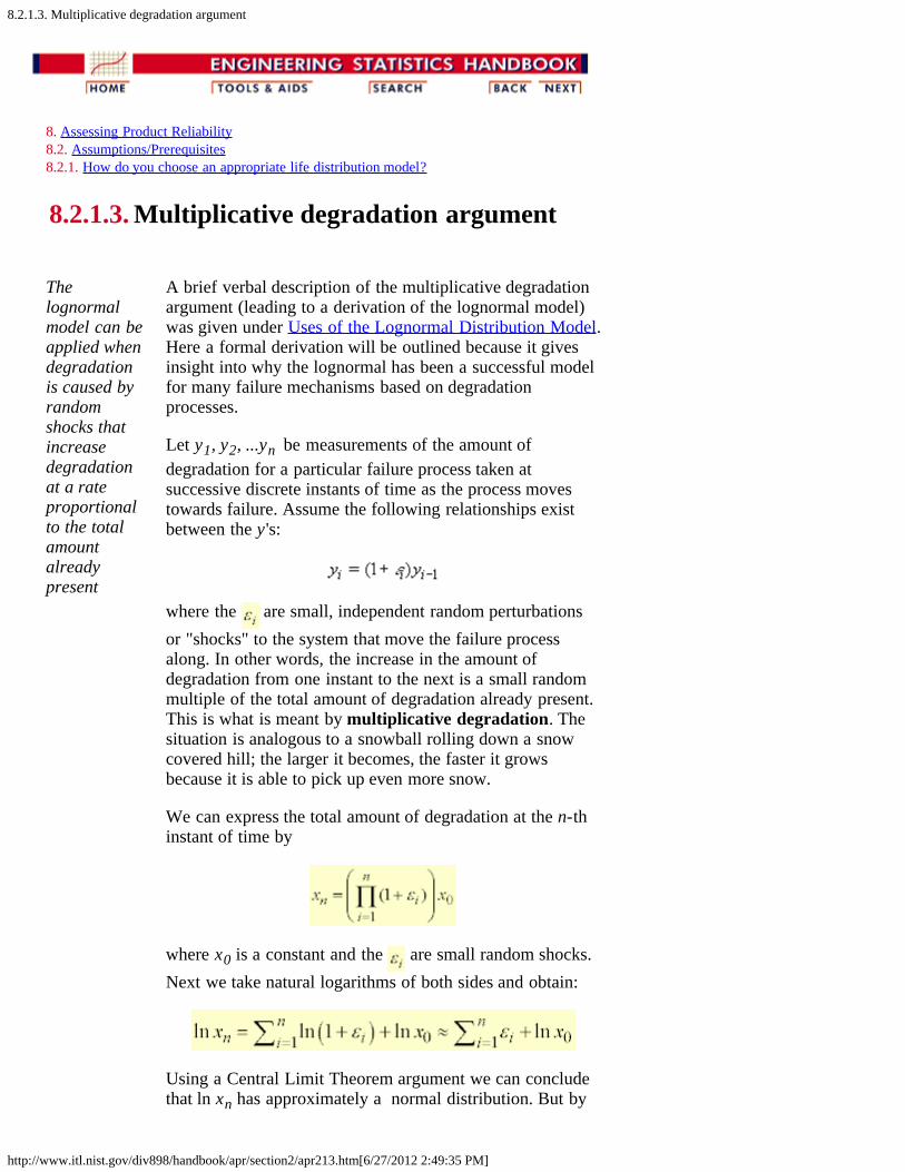
8.2.1.3. Multiplicative degradation argument
http://www.itl.nist.gov/div898/handbook/apr/section2/apr213.htm[6/27/2012 2:49:35 PM]
8. Assessing Product Reliability 8.2. Assumptions/Prerequisites 8.2.1. How do you choose an appropriate life distribution model?
8.2.1.3. Multiplicative degradation argument
Thelognormalmodel can beapplied whendegradationis caused byrandomshocks thatincreasedegradationat a rateproportionalto the totalamountalreadypresent
A brief verbal description of the multiplicative degradationargument (leading to a derivation of the lognormal model)was given under Uses of the Lognormal Distribution Model.Here a formal derivation will be outlined because it givesinsight into why the lognormal has been a successful modelfor many failure mechanisms based on degradationprocesses.
Let y1, y2, ...yn be measurements of the amount ofdegradation for a particular failure process taken atsuccessive discrete instants of time as the process movestowards failure. Assume the following relationships existbetween the y 's:
where the are small, independent random perturbationsor "shocks" to the system that move the failure processalong. In other words, the increase in the amount ofdegradation from one instant to the next is a small randommultiple of the total amount of degradation already present.This is what is meant by multiplicative degradation. Thesituation is analogous to a snowball rolling down a snowcovered hill; the larger it becomes, the faster it growsbecause it is able to pick up even more snow.
We can express the total amount of degradation at the n-thinstant of time by
where x0 is a constant and the are small random shocks.Next we take natural logarithms of both sides and obtain:
Using a Central Limit Theorem argument we can concludethat ln xn has approximately a normal distribution. But by

8.2.1.3. Multiplicative degradation argument
http://www.itl.nist.gov/div898/handbook/apr/section2/apr213.htm[6/27/2012 2:49:35 PM]
the properties of the lognormal distribution, this means thatxn (or the amount of degradation) will follow approximatelya lognormal model for any n (or at any time t). Since failureoccurs when the amount of degradation reaches a criticalpoint, time of failure will be modeled successfully by alognormal for this type of process.
Failuremechanismsthat might besuccessfullymodeled bythelognormaldistributionbased on themultiplicativedegradationmodel
What kinds of failure mechanisms might be expected tofollow a multiplicative degradation model? The processeslisted below are likely candidates:
1. Chemical reactions leading to the formation of newcompounds
2. Diffusion or migration of ions 3. Crack growth or propagation
Many semiconductor failure modes are caused by one ofthese three degradation processes. Therefore, it is nosurprise that the lognormal model has been very successfulfor the following semiconductor wear out failuremechanisms:
1. Corrosion2. Metal migration3. Electromigration4. Diffusion5. Crack growth

8.2.1.4. Fatigue life (Birnbaum-Saunders) model
http://www.itl.nist.gov/div898/handbook/apr/section2/apr214.htm[6/27/2012 2:49:35 PM]
8. Assessing Product Reliability 8.2. Assumptions/Prerequisites 8.2.1. How do you choose an appropriate life distribution model?
8.2.1.4. Fatigue life (Birnbaum-Saunders) model
A modelderivedfromrandomcrackgrowthoccurringduringmanyindependentcycles ofstress
The derivation of the Fatigue Life model is based on repeatedcycles of stress causing degradation leading to eventualfailure. The typical example is crack growth. One keyassumption is that the amount of degradation during anycycle is independent of the degradation in any other cycle,with the same random distribution.
When this assumption matches well with a hypothesizedphysical model describing the degradation process, one wouldexpect the Birnbaum-Saunders model to be a reasonabledistribution model candidate. (See the note in the derivationfor comments about the difference between the lognormalmodel derivation and the Fatigue Life model assumptions.Also see the comment on Miner's Rule).
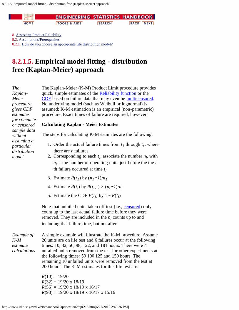
8.2.1.5. Empirical model fitting - distribution free (Kaplan-Meier) approach
http://www.itl.nist.gov/div898/handbook/apr/section2/apr215.htm[6/27/2012 2:49:36 PM]
8. Assessing Product Reliability8.2. Assumptions/Prerequisites8.2.1. How do you choose an appropriate life distribution model?
8.2.1.5. Empirical model fitting - distributionfree (Kaplan-Meier) approach
TheKaplan-Meierproceduregives CDFestimatesfor completeor censoredsample datawithoutassuming aparticulardistributionmodel
The Kaplan-Meier (K-M) Product Limit procedure providesquick, simple estimates of the Reliability function or theCDF based on failure data that may even be multicensored.No underlying model (such as Weibull or lognormal) isassumed; K-M estimation is an empirical (non-parametric)procedure. Exact times of failure are required, however.
Calculating Kaplan - Meier Estimates
The steps for calculating K-M estimates are the following:
1. Order the actual failure times from t1 through tr, wherethere are r failures
2. Corresponding to each ti, associate the number ni, withni = the number of operating units just before the the i-th failure occurred at time ti
3. Estimate R(t1) by (n1 -1)/n1
4. Estimate R(ti) by R(ti-1) × (ni -1)/ni
5. Estimate the CDF F(ti) by 1 - R(ti)
Note that unfailed units taken off test (i.e., censored) onlycount up to the last actual failure time before they wereremoved. They are included in the ni counts up to andincluding that failure time, but not after.
Example ofK-Mestimatecalculations
A simple example will illustrate the K-M procedure. Assume20 units are on life test and 6 failures occur at the followingtimes: 10, 32, 56, 98, 122, and 181 hours. There were 4unfailed units removed from the test for other experiments atthe following times: 50 100 125 and 150 hours. Theremaining 10 unfailed units were removed from the test at200 hours. The K-M estimates for this life test are:
R(10) = 19/20 R(32) = 19/20 x 18/19 R(56) = 19/20 x 18/19 x 16/17 R(98) = 19/20 x 18/19 x 16/17 x 15/16
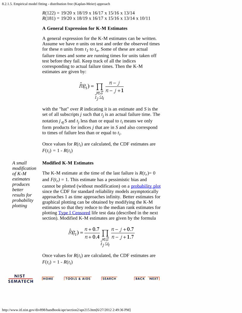
8.2.1.5. Empirical model fitting - distribution free (Kaplan-Meier) approach
http://www.itl.nist.gov/div898/handbook/apr/section2/apr215.htm[6/27/2012 2:49:36 PM]
R(122) = 19/20 x 18/19 x 16/17 x 15/16 x 13/14 R(181) = 19/20 x 18/19 x 16/17 x 15/16 x 13/14 x 10/11
A General Expression for K-M Estimates
A general expression for the K-M estimates can be written.Assume we have n units on test and order the observed timesfor these n units from t1 to tn. Some of these are actualfailure times and some are running times for units taken offtest before they fail. Keep track of all the indicescorresponding to actual failure times. Then the K-Mestimates are given by:
with the "hat" over R indicating it is an estimate and S is theset of all subscripts j such that tj is an actual failure time. Thenotation j S and tj less than or equal to ti means we onlyform products for indices j that are in S and also correspondto times of failure less than or equal to ti.
Once values for R(ti) are calculated, the CDF estimates are F(ti) = 1 - R(ti)
A smallmodificationof K-Mestimatesproducesbetterresults forprobabilityplotting
Modified K-M Estimates
The K-M estimate at the time of the last failure is R(tr)= 0and F(tr) = 1. This estimate has a pessimistic bias andcannot be plotted (without modification) on a probability plotsince the CDF for standard reliability models asymptoticallyapproaches 1 as time approaches infinity. Better estimates forgraphical plotting can be obtained by modifying the K-Mestimates so that they reduce to the median rank estimates forplotting Type I Censored life test data (described in the nextsection). Modified K-M estimates are given by the formula
Once values for R(ti) are calculated, the CDF estimates areF(ti) = 1 - R(ti)

8.2.2. How do you plot reliability data?
http://www.itl.nist.gov/div898/handbook/apr/section2/apr22.htm[6/27/2012 2:49:37 PM]
8. Assessing Product Reliability 8.2. Assumptions/Prerequisites
8.2.2. How do you plot reliability data?
Create aprobabilityplot and if thepoints line upapproximatelyon a straightline, theassumedmodel is areasonable fit
Graphical plots of reliability data are quick, useful visualtests of whether a particular model is consistent with theobserved data. The basic idea behind virtually all graphicalplotting techniques is the following:
Points calculated from the data are plotted on alog-log scale and, as long as they line upapproximately on a straight line, the analystcan conclude that the data are consistent withthe assumed model.
If the reliability data consist of (possibly multicensored)failure data from a non repairable population (or arepairable population for which only time to the first failureis considered) then the models are life distribution modelssuch as the exponential, Weibull or lognormal. If the dataconsist of repair times for a repairable system, then themodel might be the NHPP Power Law and the plot wouldbe a Duane Plot.
The kinds of plots we will consider for failure data fromnon-repairable populations are:
Probability (CDF) plotsHazard and Cum Hazard plots
For repairable populations we have
Trend plots (to check whether an HPP or exponentialmodel applies)Duane plots (to check whether the NHPP Power Lawapplies)
Later on (Section 8.4.2.1) we will also look at plots thatcan be used to check acceleration model assumptions.
Note: Many of the plots discussed in this section can alsobe used to obtain quick estimates of model parameters.This will be covered in later sections. While there may beother, more accurate ways of estimating parameters, simplegraphical estimates can be very handy, especially whenother techniques require software programs that are notreadily available.

8.2.2. How do you plot reliability data?
http://www.itl.nist.gov/div898/handbook/apr/section2/apr22.htm[6/27/2012 2:49:37 PM]

8.2.2.1. Probability plotting
http://www.itl.nist.gov/div898/handbook/apr/section2/apr221.htm[6/27/2012 2:49:38 PM]
8. Assessing Product Reliability 8.2. Assumptions/Prerequisites 8.2.2. How do you plot reliability data?
8.2.2.1. Probability plotting
Useprobabilityplots to seeyour dataand visuallycheckmodelassumptions
Probability plots are simple visual ways of summarizing reliability data by plottingCDF estimates versus time using a log-log scale.
The x axis is labeled "Time" and the y axis is labeled "cumulative percent" or"percentile". There are rules, independent of the model, for calculating plottingpositions (points) from the reliability data. These only depend on the type ofcensoring in the data and whether exact times of failure are recorded or only readouttimes.
Plot eachfailuremodeseparately
Remember that different failure modes can and should be separated out andindividually analyzed. When analyzing failure mode A, for example, treat failuretimes from failure modes B, C, etc., as censored run times. Then repeat for failuremode B, and so on.
Data pointsline uproughly ona straightline whenthe modelchosen isreasonable
When the points are plotted, the analyst fits a straight line to the data (either by eye,or with the aid of a least squares fitting program). Every straight line on, say, aWeibull probability plot uniquely corresponds to a particular Weibull lifedistribution model and the same is true for lognormal or exponential plots. If thepoints follow the line reasonably well, then the model is consistent with the data. Ifit was your previously chosen model, there is no reason to question the choice. Inaddition, there is a simple way to find the parameter estimates that correspond to thefitted straight line.
Plottingpositions onthe x axisdepend onthe type ofdatacensoring
Plotting Positions: Censored Data (Type I or Type II)
At the time ti of the i-th failure, we need an estimate of the CDF (or the cumulativepopulation percent failure). The simplest and most obvious estimate is just 100 × i/n(with a total of n units on test). This, however, is generally an overestimate (i.e.biased). Various texts recommend corrections such as 100 × (i-0.5)/n or 100 ×i/(n+1). Here, we recommend what are known as (approximate) median rankestimates.
For each time ti of the i-th failure, calculate the CDF or percentile estimate using100 × (i - 0.3)/(n + 0.4).
Plotting Positions: Readout Data
Let the readout times be T1, T2, ..., Tk and let the corresponding new failuresrecorded at each readout be r1, r2, ..., rk. Again, there are n units on test.
For each readout time Tj, calculate the CDF or percentile estimate using
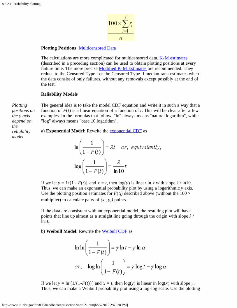
8.2.2.1. Probability plotting
http://www.itl.nist.gov/div898/handbook/apr/section2/apr221.htm[6/27/2012 2:49:38 PM]
Plotting Positions: Multicensored Data
The calculations are more complicated for multicensored data. K-M estimates(described in a preceding section) can be used to obtain plotting positions at everyfailure time. The more precise Modified K-M Estimates are recommended. Theyreduce to the Censored Type I or the Censored Type II median rank estimates whenthe data consist of only failures, without any removals except possibly at the end ofthe test.
Reliability Models
Plottingpositions onthe y axisdepend onthereliabilitymodel
The general idea is to take the model CDF equation and write it in such a way that afunction of F(t) is a linear equation of a function of t. This will be clear after a fewexamples. In the formulas that follow, "ln" always means "natural logarithm", while"log" always means "base 10 logarithm".
a) Exponential Model: Rewrite the exponential CDF as
If we let y = 1/{1 - F(t)} and x = t, then log(y) is linear in x with slope λ / ln10.Thus, we can make an exponential probability plot by using a logarithmic y axis.Use the plotting position estimates for F(ti) described above (without the 100 ×multiplier) to calculate pairs of (xi, yi) points.
If the data are consistent with an exponential model, the resulting plot will havepoints that line up almost as a straight line going through the origin with slope λ /ln10.
b) Weibull Model: Rewrite the Weibull CDF as
If we let y = ln [1/{1-F(t)}] and x = t, then log(y) is linear in log(x) with slope γ.Thus, we can make a Weibull probability plot using a log-log scale. Use the plotting
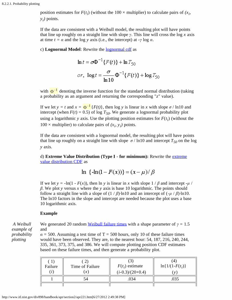
8.2.2.1. Probability plotting
http://www.itl.nist.gov/div898/handbook/apr/section2/apr221.htm[6/27/2012 2:49:38 PM]
position estimates for F(ti) (without the 100 × multiplier) to calculate pairs of (xi,yi) points.
If the data are consistent with a Weibull model, the resulting plot will have pointsthat line up roughly on a straight line with slope γ. This line will cross the log x axisat time t = α and the log y axis (i.e., the intercept) at -γ log α.
c) Lognormal Model: Rewrite the lognormal cdf as
with denoting the inverse function for the standard normal distribution (takinga probability as an argument and returning the corresponding "z" value).
If we let y = t and x = {F(t)}, then log y is linear in x with slope σ / ln10 andintercept (when F(t) = 0.5) of log T50. We generate a lognormal probability plotusing a logarithmic y axis. Use the plotting position estimates for F(ti) (without the100 × multiplier) to calculate pairs of (xi, yi) points.
If the data are consistent with a lognormal model, the resulting plot will have pointsthat line up roughly on a straight line with slope σ / ln10 and intercept T50 on the logy axis.
d) Extreme Value Distribution (Type I - for minimum): Rewrite the extremevalue distribution CDF as
If we let y = -ln(1 - F(x)), then ln y is linear in x with slope 1 / β and intercept -μ /β. We plot y versus x where the y axis is base 10 logarithmic. The points shouldfollow a straight line with a slope of (1 / β)·ln10 and an intercept of (-μ / β)·ln10.The ln10 factors in the slope and intercept are needed because the plot uses a base10 logarithmic axis.
Example
A Weibullexample ofprobabilityplotting
We generated 20 random Weibull failure times with a shape parameter of γ = 1.5and α = 500. Assuming a test time of T = 500 hours, only 10 of these failure timeswould have been observed. They are, to the nearest hour: 54, 187, 216, 240, 244,335, 361, 373, 375, and 386. We will compute plotting position CDF estimatesbased on these failure times, and then generate a probability plot.
( 1) Failure
(i)
( 2) Time of Failure
(x)
(3) F(ti) estimate (i-0.3)/(20+0.4)
(4) ln{1/(1-F(ti)}
(y)1 54 .034 .035

8.2.2.1. Probability plotting
http://www.itl.nist.gov/div898/handbook/apr/section2/apr221.htm[6/27/2012 2:49:38 PM]
2 187 .083 .0873 216 .132 .1424 240 .181 .2005 244 .230 .2626 335 .279 .3287 361 .328 .3988 373 .377 .4749 375 .426 .55610 386 .475 .645
We generate a probability plot using column (4) versus column (2) and log-log scaleaxes.
Note that the configuration of points appears to have some curvature. This is mostlydue to the very first point on the plot (the earliest time of failure). The first fewpoints on a probability plot have more variability than points in the central rangeand less attention should be paid to them when visually testing for "straightness".
Use of leastsquares(regression)to fit a linethrough thepoints on a
Since our data are plotted on a log-log scale, we fit a straight line using log(x) as theindependent variable and log(y) as the dependent variable.
The regression produces a slope estimate of 1.46, which is close to the 1.5 valueused in the simulation. The intercept is -4.114 and setting this equal to -γ log α weestimate α = 657 (the "true" value used in the simulation was 500).

8.2.2.1. Probability plotting
http://www.itl.nist.gov/div898/handbook/apr/section2/apr221.htm[6/27/2012 2:49:38 PM]
probabilityplot The analyses in this section can can be implemented using both Dataplot code and
R code. Both packages have special functions to automatically generate probabilityplots for a wide variety of distributions.

8.2.2.2. Hazard and cumulative hazard plotting
http://www.itl.nist.gov/div898/handbook/apr/section2/apr222.htm[6/27/2012 2:49:39 PM]
8. Assessing Product Reliability 8.2. Assumptions/Prerequisites 8.2.2. How do you plot reliability data?
8.2.2.2. Hazard and cumulative hazard plotting
CumulativeHazardPlottinghas thesamepurpose asprobabilityplotting
Similar to probability plots, cumulative hazard plots are used for visuallyexamining distributional model assumptions for reliability data and havea similar interpretation as probability plots. The cumulative hazard plotconsists of a plot of the cumulative hazard H(ti) versus the time ti of thei-th failure. As with probability plots, the plotting positions arecalculated independently of the model and a reasonable straight-line fitto the points confirms that the chosen model and the data are consistent.
Advantages of Cumulative Hazard Plotting
1. It is much easier to calculate plotting positions for multicensoreddata using cumulative hazard plotting techniques.
2. The most common reliability distributions, the exponential and theWeibull, are easily plotted.
Disadvantages of Cumulative Hazard Plotting
1. It is less intuitively clear just what is being plotted. In aprobability plot, the cumulative percent failed is meaningful andthe resulting straight-line fit can be used to identify times whendesired percentages of the population will have failed. The percentcumulative hazard can increase beyond 100 % and is harder tointerpret.
2. Normal cumulative hazard plotting techniques require exact timesof failure and running times.
3. Since computers are able to calculate K-M estimates forprobability plotting, the main advantage of cumulative hazardplotting goes away.
Since probability plots are generally more useful, we will only give abrief description of hazard plotting.
How to Make Cumulative Hazard Plots
1. Order the failure times and running times for each of the n units ontest in ascending order from 1 to n. The order is called the rank ofthe unit. Calculate the reverse rank for each unit (reverse rank = n-rank +1).
2. Calculate a hazard "value" for every failed unit (do this only forthe failed units). The hazard value for the failed unit with reverserank k is just 1/k.
3. Calculate the cumulative hazard values for each failed unit. The
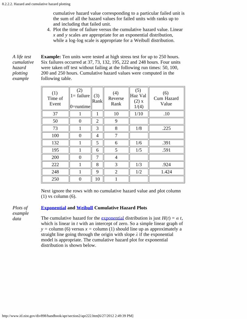
8.2.2.2. Hazard and cumulative hazard plotting
http://www.itl.nist.gov/div898/handbook/apr/section2/apr222.htm[6/27/2012 2:49:39 PM]
cumulative hazard value corresponding to a particular failed unit isthe sum of all the hazard values for failed units with ranks up toand including that failed unit.
4. Plot the time of failure versus the cumulative hazard value. Linearx and y scales are appropriate for an exponential distribution,while a log-log scale is appropriate for a Weibull distribution.
A life testcumulativehazardplottingexample
Example: Ten units were tested at high stress test for up to 250 hours.Six failures occurred at 37, 73, 132, 195, 222 and 248 hours. Four unitswere taken off test without failing at the following run times: 50, 100,200 and 250 hours. Cumulative hazard values were computed in thefollowing table.
(1) Time ofEvent
(2) 1= failure
0=runtime
(3) Rank
(4) Reverse
Rank
(5) Haz Val
(2) x1/(4)
(6) Cum Hazard
Value
37 1 1 10 1/10 .1050 0 2 9 73 1 3 8 1/8 .225100 0 4 7 132 1 5 6 1/6 .391195 1 6 5 1/5 .591200 0 7 4 222 1 8 3 1/3 .924248 1 9 2 1/2 1.424250 0 10 1
Next ignore the rows with no cumulative hazard value and plot column(1) vs column (6).
Plots ofexampledata
Exponential and Weibull Cumulative Hazard Plots
The cumulative hazard for the exponential distribution is just H(t) = α t,which is linear in t with an intercept of zero. So a simple linear graph ofy = column (6) versus x = column (1) should line up as approximately astraight line going through the origin with slope λ if the exponentialmodel is appropriate. The cumulative hazard plot for exponentialdistribution is shown below.
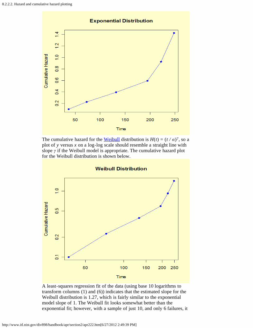
8.2.2.2. Hazard and cumulative hazard plotting
http://www.itl.nist.gov/div898/handbook/apr/section2/apr222.htm[6/27/2012 2:49:39 PM]
The cumulative hazard for the Weibull distribution is H(t) = (t / α)γ, so aplot of y versus x on a log-log scale should resemble a straight line withslope γ if the Weibull model is appropriate. The cumulative hazard plotfor the Weibull distribution is shown below.
A least-squares regression fit of the data (using base 10 logarithms totransform columns (1) and (6)) indicates that the estimated slope for theWeibull distribution is 1.27, which is fairly similar to the exponentialmodel slope of 1. The Weibull fit looks somewhat better than theexponential fit; however, with a sample of just 10, and only 6 failures, it

8.2.2.2. Hazard and cumulative hazard plotting
http://www.itl.nist.gov/div898/handbook/apr/section2/apr222.htm[6/27/2012 2:49:39 PM]
is difficult to pick a model from the data alone.
Software The analyses in this section can can be implemented using both Dataplotcode and R code.

8.2.2.3. Trend and growth plotting (Duane plots)
http://www.itl.nist.gov/div898/handbook/apr/section2/apr223.htm[6/27/2012 2:49:41 PM]
8. Assessing Product Reliability 8.2. Assumptions/Prerequisites 8.2.2. How do you plot reliability data?
8.2.2.3. Trend and growth plotting (Duane plots)
Repair ratesare typicallyeither nearlyconstantover time orelseconsistentlyfollow agood or abad trend
Models for repairable systems were described earlier. These models arefor the cumulative number of failuress (or the repair rate) over time. Thetwo models used with most success throughout industry are the HPP(constant repair rate or "exponential" system model) and the NHPPPower Law process (the repair rate is the polynomial m(t) = αt -β ).
Before constructing a Duane Plot, there are a few simple trend plots thatoften convey strong evidence of the presence or absence of a trend in therepair rate over time. If there is no trend, an HPP model is reasonable. Ifthere is an apparent improvement or degradation trend, a Duane Plot willprovide a visual check for whether the NHPP Power law model isconsistent with the data.
A few simpleplots canhelp usdecidewhethertrends arepresent
These simple visual graphical tests for trends are
1. Plot cumulative failures versus system age (a step function thatgoes up every time there is a new failure). If this plot looks linear,there is no obvious improvement (or degradation) trend. A bendingdownward indicates improvement; bending upward indicatesdegradation.
2. Plot the inter arrival times between new failures (in other words,the waiting times between failures, with the time to the first failureused as the first "inter-arrival" time). If these trend up, there isimprovement; if they trend down, there is degradation.
3. Plot the reciprocals of the inter-arrival times. Each reciprocal is anew failure rate estimate based only on the waiting time since thelast failure. If these trend down, there is improvement; an upwardtrend indicates degradation.
Trend plotsand a DuanePlot foractualReliabilityImprovementTest data
Case Study 1: Use of Trend Plots and Duane Plots with ReliabilityImprovement Test Data
A prototype of a new, complex piece of equipment went through a 1500operational hours Reliability Improvement Test. During the test therewere 10 failures. As part of the improvement process, a cross functionalFailure Review Board made sure every failure was analyzed down to theroot cause and design and parts selection fixes were implemented on theprototype. The observed failure times were: 5, 40, 43, 175, 389, 712, 747,795, 1299 and 1478 hours, with the test ending at 1500 hours. Thereliability engineer on the Failure Review Board first made trend plots asdescribed above, then made a Duane plot. These plots follow.
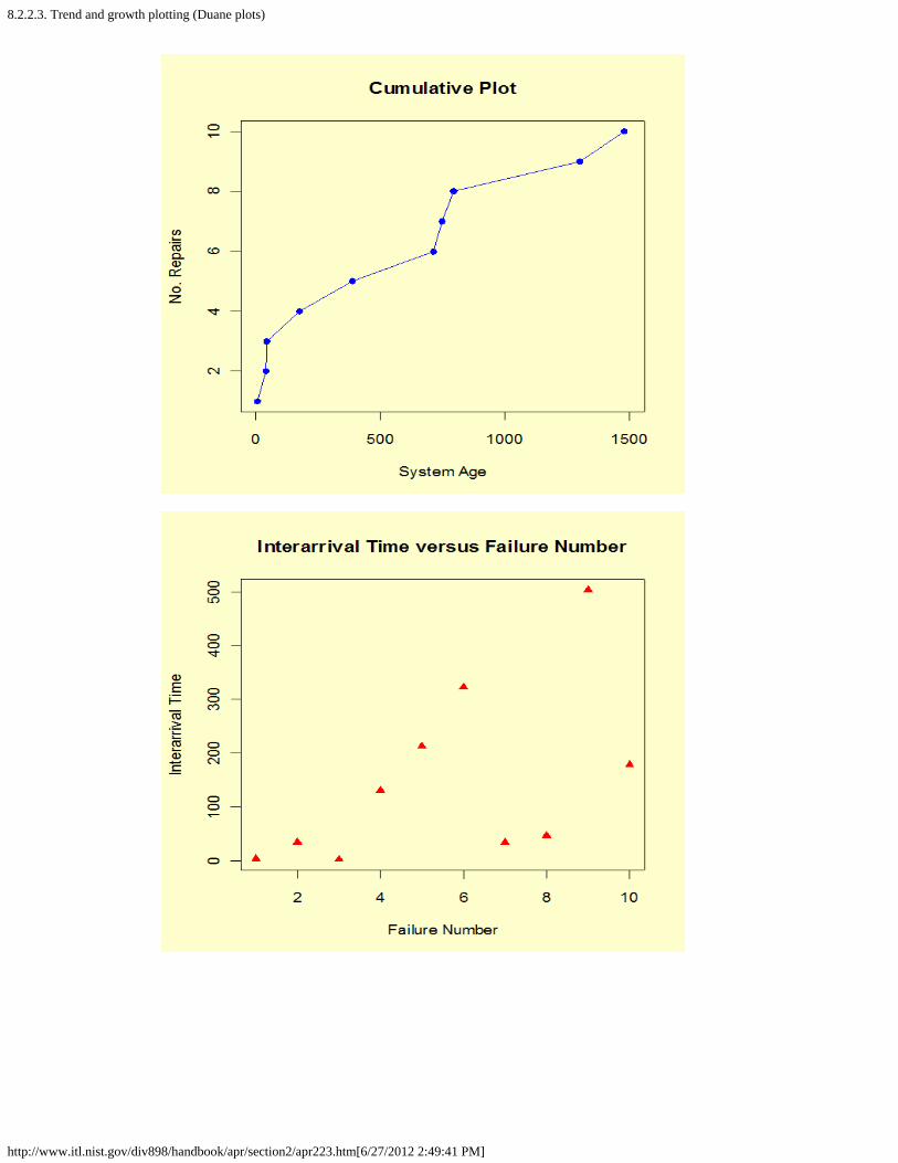
8.2.2.3. Trend and growth plotting (Duane plots)
http://www.itl.nist.gov/div898/handbook/apr/section2/apr223.htm[6/27/2012 2:49:41 PM]
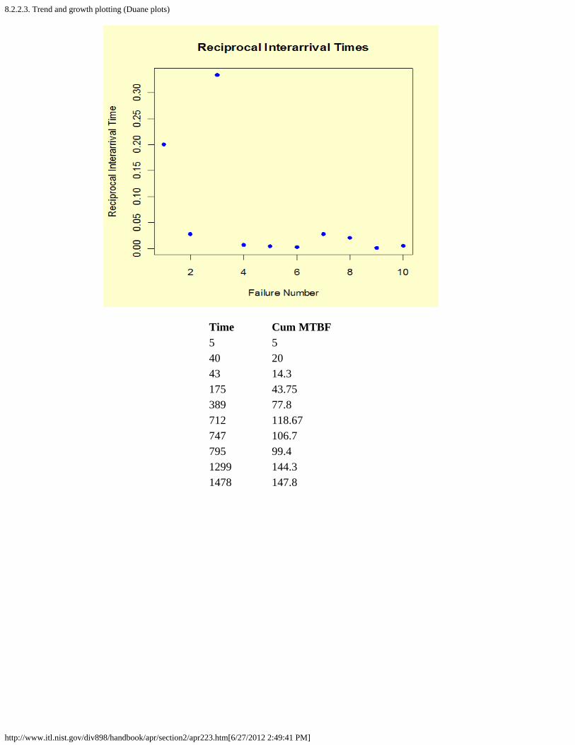
8.2.2.3. Trend and growth plotting (Duane plots)
http://www.itl.nist.gov/div898/handbook/apr/section2/apr223.htm[6/27/2012 2:49:41 PM]
Time Cum MTBF5 540 2043 14.3175 43.75389 77.8712 118.67747 106.7795 99.41299 144.31478 147.8
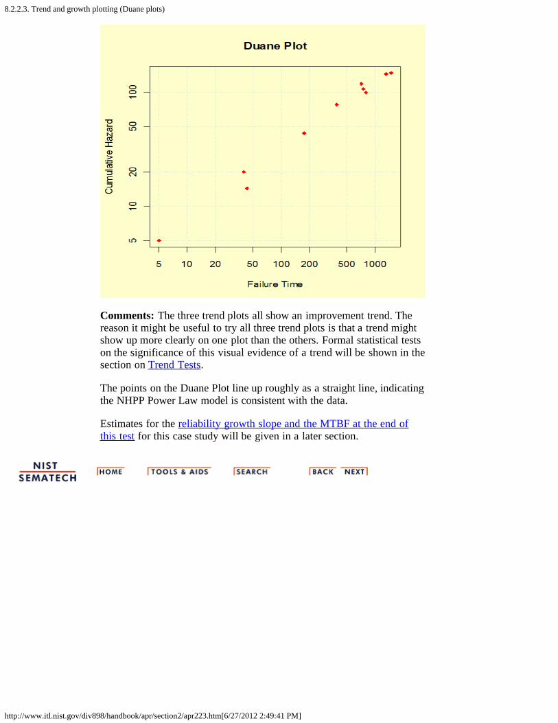
8.2.2.3. Trend and growth plotting (Duane plots)
http://www.itl.nist.gov/div898/handbook/apr/section2/apr223.htm[6/27/2012 2:49:41 PM]
Comments: The three trend plots all show an improvement trend. Thereason it might be useful to try all three trend plots is that a trend mightshow up more clearly on one plot than the others. Formal statistical testson the significance of this visual evidence of a trend will be shown in thesection on Trend Tests.
The points on the Duane Plot line up roughly as a straight line, indicatingthe NHPP Power Law model is consistent with the data.
Estimates for the reliability growth slope and the MTBF at the end ofthis test for this case study will be given in a later section.

8.2.3. How can you test reliability model assumptions?
http://www.itl.nist.gov/div898/handbook/apr/section2/apr23.htm[6/27/2012 2:49:42 PM]
8. Assessing Product Reliability 8.2. Assumptions/Prerequisites
8.2.3. How can you test reliability modelassumptions?
Modelsarefrequentlynecessary- butshouldalways bechecked
Since reliability models are often used to project (extrapolate)failure rates or MTBF's that are well beyond the range of thereliability data used to fit these models, it is very important to"test" whether the models chosen are consistent with whateverdata are available. This section describes several ways ofdeciding whether a model under examination is acceptable.These are:
1. Visual Tests2. Goodness of Fit Tests3. Likelihood Ratio Tests4. Trend Tests

8.2.3.1. Visual tests
http://www.itl.nist.gov/div898/handbook/apr/section2/apr231.htm[6/27/2012 2:49:43 PM]
8. Assessing Product Reliability 8.2. Assumptions/Prerequisites 8.2.3. How can you test reliability model assumptions?
8.2.3.1. Visual tests
A visualtest of amodel is asimple plotthat tells usat a glancewhether themodel isconsistentwith thedata
We have already seen many examples of visual tests ofmodels. These were: Probability Plots, Cum hazard Plots,Duane Plots and Trend Plots. In all but the Trend Plots, themodel was "tested' by how well the data points followed astraight line. In the case of the Trend Plots, we looked forcurvature away from a straight line (cum repair plots) orincreasing or decreasing size trends (inter arrival times andreciprocal inter-arrival times).
These simple plots are a powerful diagnostic tool since thehuman eye can often detect patterns or anomalies in the databy studying graphs. That kind of invaluable informationwould be lost if the analyst only used quantitative statisticaltests to check model fit. Every analysis should include asmany visual tests as are applicable.
Advantages of Visual Tests
1. Easy to understand and explain.2. Can occasionally reveal patterns or anomalies in the
data.3. When a model "passes" a visual test, it is somewhat
unlikely any quantitative statistical test will "reject" it(the human eye is less forgiving and more likely todetect spurious trends)
Combinevisual testswith formalquantitativetests for the"best ofbothworlds"approach
Disadvantages of Visual Tests
1. Visual tests are subjective.2. They do not quantify how well or how poorly a model
fits the data.3. They are of little help in choosing between two or more
competing models that both appear to fit the data.4. Simulation studies have shown that correct models may
often appear to not fit well by sheer chance - it is hardto know when visual evidence is strong enough toreject what was previously believed to be a correctmodel.
You can retain the advantages of visual tests and removetheir disadvantages by combining data plots with formal

8.2.3.1. Visual tests
http://www.itl.nist.gov/div898/handbook/apr/section2/apr231.htm[6/27/2012 2:49:43 PM]
statistical tests of goodness of fit or trend.
8.2.3.2. Goodness of fit tests
http://www.itl.nist.gov/div898/handbook/apr/section2/apr232.htm[6/27/2012 2:49:43 PM]
8. Assessing Product Reliability 8.2. Assumptions/Prerequisites 8.2.3. How can you test reliability model assumptions?
8.2.3.2. Goodness of fit tests
AGoodnessof Fit testchecks onwhetheryour dataarereasonableor highlyunlikely,given anassumeddistributionmodel
General tests for checking the hypothesis that your data areconsistent with a particular model are discussed in Chapter 7.Details and examples of the Chi-Square Goodness of Fit testand the Kolmolgorov-Smirnov (K-S) test are given inChapter 1. The Chi-Square test can be used with Type I orType II censored data and readout data if there are enoughfailures and readout times. The K-S test generally requirescomplete samples, which limits its usefulness in reliabilityanalysis.
These tests control the probability of rejecting a valid modelas follows:
the analyst chooses a confidence level designated by100 × (1 - ).a test statistic is calculated from the data and comparedto likely values for this statistic, assuming the model iscorrect. if the test statistic has a very unlikely value, or less thanor equal to an probability of occurring, where is asmall value like .1 or .05 or even .01, then the model isrejected.
So the risk of rejecting the right model is kept to or less,and the choice of usually takes into account the potentialloss or difficulties incurred if the model is rejected.
8.2.3.3. Likelihood ratio tests
http://www.itl.nist.gov/div898/handbook/apr/section2/apr233.htm[6/27/2012 2:49:44 PM]
8. Assessing Product Reliability 8.2. Assumptions/Prerequisites 8.2.3. How can you test reliability model assumptions?
8.2.3.3. Likelihood ratio tests
LikelihoodRatio Testsare apowerful,very generalmethod oftestingmodelassumptions.However, they requirespecialsoftware,not alwaysreadilyavailable.
Likelihood functions for reliability data are described inSection 4. Two ways we use likelihood functions to choosemodels or verify/validate assumptions are:
1. Calculate the maximum likelihood of the sample databased on an assumed distribution model (the maximumoccurs when unknown parameters are replaced by theirmaximum likelihood estimates). Repeat this calculation forother candidate distribution models that also appear to fit thedata (based on probability plots). If all the models have thesame number of unknown parameters, and there is noconvincing reason to choose one particular model overanother based on the failure mechanism or previoussuccessful analyses, then pick the model with the largestlikelihood value.
2. Many model assumptions can be viewed as puttingrestrictions on the parameters in a likelihood expression thateffectively reduce the total number of unknown parameters.Some common examples are:
Exampleswhereassumptionscan betested by theLikelihoodRatio Test
i) It is suspected that a type of data, typicallymodeled by a Weibull distribution, can be fitadequately by an exponential model. Theexponential distribution is a special case of theWeibull, with the shape parameter set to 1. Ifwe write the Weibull likelihood function for thedata, the exponential model likelihood functionis obtained by setting to 1, and the number ofunknown parameters has been reduced from twoto one.
ii) Assume we have n cells of data from anacceleration test, with each cell having adifferent operating temperature. We assume alognormal population model applies in everycell. Without an acceleration model assumption,the likelihood of the experimental data would bethe product of the likelihoods from each celland there would be 2n unknown parameters (adifferent T50 and for each cell). If we assumean Arrhenius model applies, the total number of
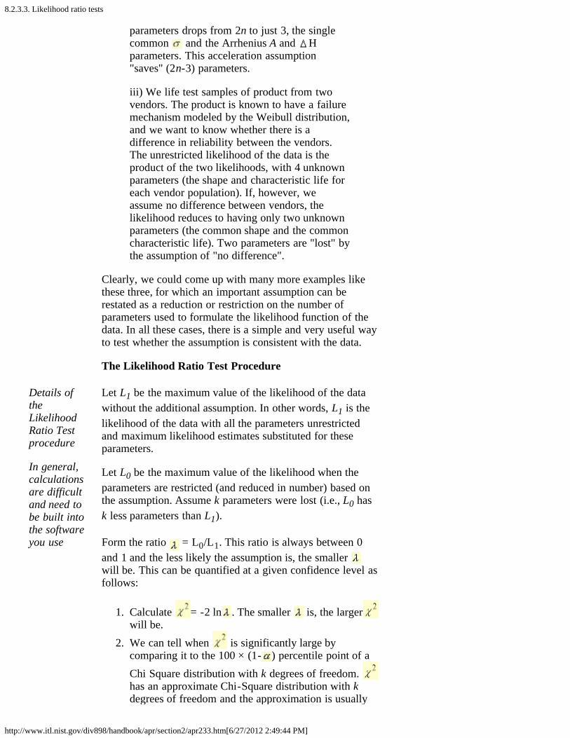
8.2.3.3. Likelihood ratio tests
http://www.itl.nist.gov/div898/handbook/apr/section2/apr233.htm[6/27/2012 2:49:44 PM]
parameters drops from 2n to just 3, the singlecommon and the Arrhenius A and Hparameters. This acceleration assumption"saves" (2n-3) parameters.
iii) We life test samples of product from twovendors. The product is known to have a failuremechanism modeled by the Weibull distribution,and we want to know whether there is adifference in reliability between the vendors.The unrestricted likelihood of the data is theproduct of the two likelihoods, with 4 unknownparameters (the shape and characteristic life foreach vendor population). If, however, weassume no difference between vendors, thelikelihood reduces to having only two unknownparameters (the common shape and the commoncharacteristic life). Two parameters are "lost" bythe assumption of "no difference".
Clearly, we could come up with many more examples likethese three, for which an important assumption can berestated as a reduction or restriction on the number ofparameters used to formulate the likelihood function of thedata. In all these cases, there is a simple and very useful wayto test whether the assumption is consistent with the data.
The Likelihood Ratio Test Procedure
Details oftheLikelihoodRatio Testprocedure
In general,calculationsare difficultand need tobe built intothe softwareyou use
Let L1 be the maximum value of the likelihood of the datawithout the additional assumption. In other words, L1 is thelikelihood of the data with all the parameters unrestrictedand maximum likelihood estimates substituted for theseparameters.
Let L0 be the maximum value of the likelihood when theparameters are restricted (and reduced in number) based onthe assumption. Assume k parameters were lost (i.e., L0 hask less parameters than L1).
Form the ratio = L0/L1. This ratio is always between 0and 1 and the less likely the assumption is, the smaller will be. This can be quantified at a given confidence level asfollows:
1. Calculate = -2 ln . The smaller is, the largerwill be.
2. We can tell when is significantly large bycomparing it to the 100 × (1- ) percentile point of aChi Square distribution with k degrees of freedom. has an approximate Chi-Square distribution with kdegrees of freedom and the approximation is usually

8.2.3.3. Likelihood ratio tests
http://www.itl.nist.gov/div898/handbook/apr/section2/apr233.htm[6/27/2012 2:49:44 PM]
good, even for small sample sizes.3. The likelihood ratio test computes and rejects the
assumption if is larger than a Chi-Squarepercentile with k degrees of freedom, where thepercentile corresponds to the confidence level chosenby the analyst.
Note: While Likelihood Ratio test procedures are veryuseful and widely applicable, the computations are difficultto perform by hand, especially for censored data, andappropriate software is necessary.

8.2.3.4. Trend tests
http://www.itl.nist.gov/div898/handbook/apr/section2/apr234.htm[6/27/2012 2:49:45 PM]
8. Assessing Product Reliability 8.2. Assumptions/Prerequisites 8.2.3. How can you test reliability model assumptions?
8.2.3.4. Trend tests
FormalTrend TestsshouldaccompanyTrend Plotsand DuanePlots. Threeare given inthis section
In this section we look at formal statistical tests that canallow us to quantitatively determine whether or not therepair times of a system show a significant trend (whichmay be an improvement or a degradation trend). Thesection on trend and growth plotting contained a discussionof visual tests for trends - this section complements thosevisual tests as several numerical tests are presented.
Three statistical test procedures will be described:
1. The Reverse Arrangement Test (a simple and usefultest that has the advantage of making no assumptionsabout a model for the possible trend)
2. The Military Handbook Test (optimal fordistinguishing between "no trend' and a trendfollowing the NHPP Power Law or Duane model)
3. The Laplace Test (optimal for distinguishing between"no trend' and a trend following the NHPPExponential Law model)
The ReverseArrangementTest (RATtest) is simpleand makes noassumptionsabout whatmodel a trendmight follow
The Reverse Arrangement Test
Assume there are r repairs during the observation periodand they occurred at system ages T1, T2, T3, ...Tr (we set thestart of the observation period to T = 0). Let I1 = T1, I2 = T2 - T1, I3 = T3 - T2, ..., Ir = Tr - Tr-1 be the inter-arrival times for repairs (i.e., the sequence of waiting timesbetween failures). Assume the observation period ends attime Tend>Tr.
Previously, we plotted this sequence of inter-arrival timesto look for evidence of trends. Now, we calculate howmany instances we have of a later inter-arrival time beingstrictly greater than an earlier inter-arrival time. Each timethat happens, we call it a reversal. If there are a lot ofreversals (more than are likely from pure chance with notrend), we have significant evidence of an improvementtrend. If there are too few reversals we have significantevidence of degradation.
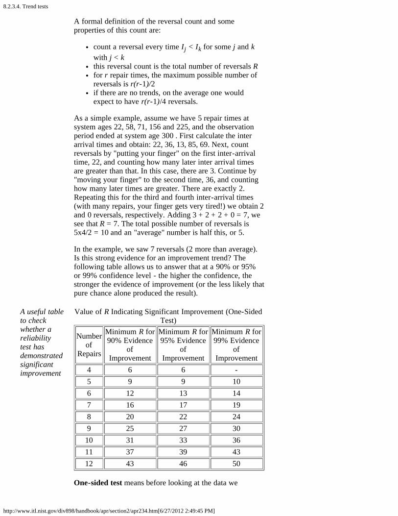
8.2.3.4. Trend tests
http://www.itl.nist.gov/div898/handbook/apr/section2/apr234.htm[6/27/2012 2:49:45 PM]
A formal definition of the reversal count and someproperties of this count are:
count a reversal every time Ij < Ik for some j and kwith j < k this reversal count is the total number of reversals Rfor r repair times, the maximum possible number ofreversals is r(r-1)/2if there are no trends, on the average one wouldexpect to have r(r-1)/4 reversals.
As a simple example, assume we have 5 repair times atsystem ages 22, 58, 71, 156 and 225, and the observationperiod ended at system age 300 . First calculate the interarrival times and obtain: 22, 36, 13, 85, 69. Next, countreversals by "putting your finger" on the first inter-arrivaltime, 22, and counting how many later inter arrival timesare greater than that. In this case, there are 3. Continue by"moving your finger" to the second time, 36, and countinghow many later times are greater. There are exactly 2.Repeating this for the third and fourth inter-arrival times(with many repairs, your finger gets very tired!) we obtain 2and 0 reversals, respectively. Adding 3 + 2 + 2 + 0 = 7, wesee that R = 7. The total possible number of reversals is5x4/2 = 10 and an "average" number is half this, or 5.
In the example, we saw 7 reversals (2 more than average).Is this strong evidence for an improvement trend? Thefollowing table allows us to answer that at a 90% or 95%or 99% confidence level - the higher the confidence, thestronger the evidence of improvement (or the less likely thatpure chance alone produced the result).
A useful tableto checkwhether areliabilitytest hasdemonstratedsignificantimprovement
Value of R Indicating Significant Improvement (One-SidedTest)
Numberof
Repairs
Minimum R for90% Evidence
ofImprovement
Minimum R for95% Evidence
ofImprovement
Minimum R for99% Evidence
ofImprovement
4 6 6 -5 9 9 106 12 13 147 16 17 198 20 22 249 25 27 30
10 31 33 3611 37 39 4312 43 46 50
One-sided test means before looking at the data we

8.2.3.4. Trend tests
http://www.itl.nist.gov/div898/handbook/apr/section2/apr234.htm[6/27/2012 2:49:45 PM]
expected improvement trends, or, at worst, a constant repairrate. This would be the case if we know of actions taken toimprove reliability (such as occur during reliabilityimprovement tests).
For the r = 5 repair times example above where we had R =7, the table shows we do not (yet) have enough evidence todemonstrate a significant improvement trend. That does notmean that an improvement model is incorrect - it just meansit is not yet "proved" statistically. With small numbers ofrepairs, it is not easy to obtain significant results.
For numbers of repairs beyond 12, there is a goodapproximation formula that can be used to determinewhether R is large enough to be significant. Calculate
Use thisformula whenthere aremore than 12repairs in thedata set
and if z > 1.282, we have at least 90% significance. If z >1.645, we have 95% significance, and a z > 2.33 indicates99% significance since z has an approximate standardnormal distribution.
That covers the (one-sided) test for significantimprovement trends. If, on the other hand, we believe theremay be a degradation trend (the system is wearing out orbeing over stressed, for example) and we want to know ifthe data confirms this, then we expect a low value for R andwe need a table to determine when the value is low enoughto be significant. The table below gives these critical valuesfor R.
Value of R Indicating Significant Degradation Trend (One-Sided Test)
Numberof
Repairs
Maximum Rfor 90%
Evidence ofDegradation
Maximum Rfor 95%
Evidence ofDegradation
Maximum Rfor 99%
Evidence ofDegradation
4 0 0 -5 1 1 06 3 2 17 5 4 28 8 6 49 11 9 6
10 14 12 911 18 16 12
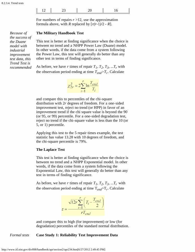
8.2.3.4. Trend tests
http://www.itl.nist.gov/div898/handbook/apr/section2/apr234.htm[6/27/2012 2:49:45 PM]
12 23 20 16
For numbers of repairs r >12, use the approximationformula above, with R replaced by [r(r-1)/2 - R].
Because ofthe success ofthe Duanemodel withindustrialimprovementtest data, thisTrend Test isrecommended
The Military Handbook Test
This test is better at finding significance when the choice isbetween no trend and a NHPP Power Law (Duane) model.In other words, if the data come from a system followingthe Power Law, this test will generally do better than anyother test in terms of finding significance.
As before, we have r times of repair T1, T2, T3, ...Tr withthe observation period ending at time Tend>Tr. Calculate
and compare this to percentiles of the chi-squaredistribution with 2r degrees of freedom. For a one-sidedimprovement test, reject no trend (or HPP) in favor of animprovement trend if the chi square value is beyond the 90(or 95, or 99) percentile. For a one-sided degradation test,reject no trend if the chi-square value is less than the 10 (or5, or 1) percentile.
Applying this test to the 5 repair times example, the teststatistic has value 13.28 with 10 degrees of freedom, andthe chi-square percentile is 79%.
The Laplace Test
This test is better at finding significance when the choice isbetween no trend and a NHPP Exponential model. In otherwords, if the data come from a system following theExponential Law, this test will generally do better than anytest in terms of finding significance.
As before, we have r times of repair T1, T2, T3, ...Tr withthe observation period ending at time Tend>Tr. Calculate
and compare this to high (for improvement) or low (fordegradation) percentiles of the standard normal distribution.
Formal tests Case Study 1: Reliability Test Improvement Data

8.2.3.4. Trend tests
http://www.itl.nist.gov/div898/handbook/apr/section2/apr234.htm[6/27/2012 2:49:45 PM]
generallyconfirm thesubjectiveinformationconveyed bytrend plots
(Continued from earlier work)
The failure data and Trend plots and Duane plot wereshown earlier. The observed failure times were: 5, 40, 43,175, 389, 712, 747, 795, 1299 and 1478 hours, with the testending at 1500 hours.
Reverse Arrangement Test: The inter-arrival times are: 5,35, 3, 132, 214, 323, 35, 48, 504 and 179. The number ofreversals is 33, which, according to the table above, is justsignificant at the 95% level.
The Military Handbook Test: The Chi-Square teststatistic, using the formula given above, is 37.23 with 20degrees of freedom and has significance level 98.9%. Sincethe Duane Plot looked very reasonable, this test probablygives the most precise significance assessment of howunlikely it is that sheer chance produced such an apparentimprovement trend (only about 1.1% probability).

8.2.4. How do you choose an appropriate physical acceleration model?
http://www.itl.nist.gov/div898/handbook/apr/section2/apr24.htm[6/27/2012 2:49:47 PM]
8. Assessing Product Reliability 8.2. Assumptions/Prerequisites
8.2.4. How do you choose an appropriatephysical acceleration model?
Choosing agoodaccelerationmodel ispart scienceand part art- but startwith a goodliteraturesearch
Choosing a physical acceleration model is a lot like choosinga life distribution model. First identify the failure mode andwhat stresses are relevant (i.e., will accelerate the failuremechanism). Then check to see if the literature containsexamples of successful applications of a particular model forthis mechanism.
If the literature offers little help, try the models described inearlier sections :
ArrheniusThe (inverse) power rule for voltageThe exponential voltage modelTwo temperature/voltage modelsThe electromigration modelThree stress models (temperature, voltage andhumidity)Eyring (for more than three stresses or when the above models are not satisfactory)The Coffin-Manson mechanical crack growth model
All but the last model (the Coffin-Manson) apply to chemicalor electronic failure mechanisms, and since temperature isalmost always a relevant stress for these mechanisms, theArrhenius model is nearly always a part of any more generalmodel. The Coffin-Manson model works well for manymechanical fatigue-related mechanisms.
Sometimes models have to be adjusted to include athreshold level for some stresses. In other words, failuremight never occur due to a particular mechanism unless aparticular stress (temperature, for example) is beyond athreshold value. A model for a temperature-dependentmechanism with a threshold at T = T0 might look like
time to fail = f(T)/(T-T0)
for which f(T) could be Arrhenius. As the temperaturedecreases towards T0, time to fail increases toward infinityin this (deterministic) acceleration model.

8.2.4. How do you choose an appropriate physical acceleration model?
http://www.itl.nist.gov/div898/handbook/apr/section2/apr24.htm[6/27/2012 2:49:47 PM]
Modelsderivedtheoreticallyhave beenverysuccessfuland areconvincing
In some cases, a mathematical/physical description of thefailure mechanism can lead to an acceleration model. Someof the models above were originally derived that way.
Simplemodels areoften thebest
In general, use the simplest model (fewest parameters) youcan. When you have chosen a model, use visual tests andformal statistical fit tests to confirm the model is consistentwith your data. Continue to use the model as long as it givesresults that "work," but be quick to look for a new modelwhen it is clear the old one is no longer adequate.
There are some good quotes that apply here:
Quotes fromexperts onmodels
"All models are wrong, but some are useful." - George Box,and the principle of Occam's Razor (attributed to the 14thcentury logician William of Occam who said “Entities shouldnot be multiplied unnecessarily” - or something equivalent tothat in Latin).
A modern version of Occam's Razor is: If you have twotheories that both explain the observed facts then you shoulduse the simplest one until more evidence comes along - alsocalled the Law of Parsimony.
Finally, for those who feel the above quotes place too muchemphasis on simplicity, there are several appropriate quotesfrom Albert Einstein:
"Make your theory as simple as possible, but nosimpler"
"For every complex question there is a simpleand wrong solution."

8.2.5. What models and assumptions are typically made when Bayesian methods are used for reliability evaluation?
http://www.itl.nist.gov/div898/handbook/apr/section2/apr25.htm[6/27/2012 2:49:48 PM]
8. Assessing Product Reliability 8.2. Assumptions/Prerequisites
8.2.5. What models and assumptions aretypically made when Bayesian methodsare used for reliability evaluation?
The basics of Bayesian methodology were explained earlier,along with some of the advantages and disadvantages ofusing this approach. Here we only consider the models andassumptions that are commonplace when applying Bayesianmethodology to evaluate system reliability.
Bayesianassumptionsfor thegammaexponentialsystemmodel
Assumptions:
1. Failure times for the system under investigation can beadequately modeled by the exponential distribution. Forrepairable systems, this means the HPP model applies and thesystem is operating in the flat portion of the bathtub curve.While Bayesian methodology can also be applied to non-repairable component populations, we will restrict ourselvesto the system application in this Handbook.
2. The MTBF for the system can be regarded as chosen froma prior distribution model that is an analytic representation ofour previous information or judgments about the system'sreliability. The form of this prior model is the gammadistribution (the conjugate prior for the exponential model).The prior model is actually defined for = 1/MTBF since itis easier to do the calculations this way.
3. Our prior knowledge is used to choose the gammaparameters a and b for the prior distribution model for .There are many possible ways to convert "knowledge" togamma parameters, depending on the form of the"knowledge" - we will describe three approaches.
Severalways tochoose thepriorgammaparametervalues
i) If you have actual data from previous testing doneon the system (or a system believed to have the samereliability as the one under investigation), this is themost credible prior knowledge, and the easiest to use.Simply set the gamma parameter a equal to the totalnumber of failures from all the previous data, and setthe parameter b equal to the total of all the previoustest hours.
ii) A consensus method for determining a and b that
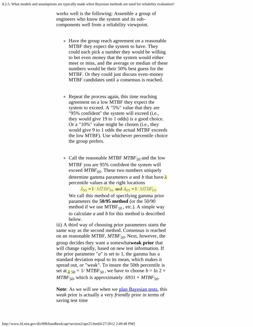
8.2.5. What models and assumptions are typically made when Bayesian methods are used for reliability evaluation?
http://www.itl.nist.gov/div898/handbook/apr/section2/apr25.htm[6/27/2012 2:49:48 PM]
works well is the following: Assemble a group ofengineers who know the system and its sub-components well from a reliability viewpoint.
Have the group reach agreement on a reasonableMTBF they expect the system to have. Theycould each pick a number they would be willingto bet even money that the system would eithermeet or miss, and the average or median of thesenumbers would be their 50% best guess for theMTBF. Or they could just discuss even-moneyMTBF candidates until a consensus is reached.
Repeat the process again, this time reachingagreement on a low MTBF they expect thesystem to exceed. A "5%" value that they are"95% confident" the system will exceed (i.e.,they would give 19 to 1 odds) is a good choice.Or a "10%" value might be chosen (i.e., theywould give 9 to 1 odds the actual MTBF exceedsthe low MTBF). Use whichever percentile choicethe group prefers.
Call the reasonable MTBF MTBF50 and the lowMTBF you are 95% confident the system willexceed MTBF05. These two numbers uniquelydetermine gamma parameters a and b that havepercentile values at the right locations
We call this method of specifying gamma priorparameters the 50/95 method (or the 50/90method if we use MTBF10 , etc.). A simple wayto calculate a and b for this method is describedbelow.
iii) A third way of choosing prior parameters starts thesame way as the second method. Consensus is reachedon an reasonable MTBF, MTBF50. Next, however, thegroup decides they want a somewhatweak prior thatwill change rapidly, based on new test information. Ifthe prior parameter "a" is set to 1, the gamma has astandard deviation equal to its mean, which makes itspread out, or "weak". To insure the 50th percentile isset at 50 = 1/ MTBF50 , we have to choose b = ln 2 ×MTBF50, which is approximately .6931 × MTBF50.
Note: As we will see when we plan Bayesian tests, thisweak prior is actually a very friendly prior in terms ofsaving test time
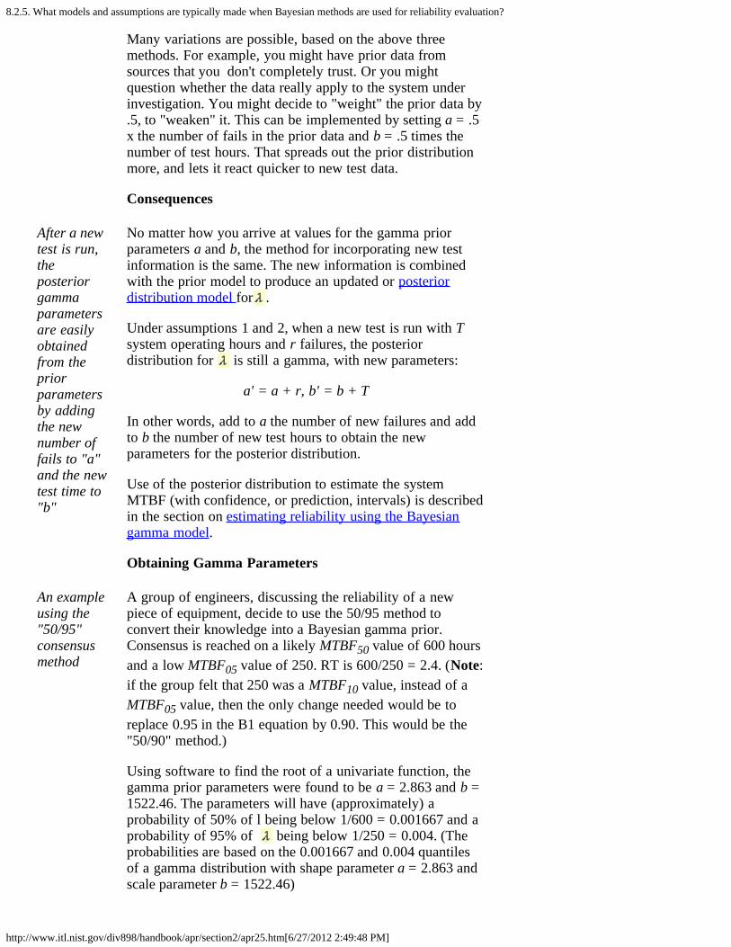
8.2.5. What models and assumptions are typically made when Bayesian methods are used for reliability evaluation?
http://www.itl.nist.gov/div898/handbook/apr/section2/apr25.htm[6/27/2012 2:49:48 PM]
Many variations are possible, based on the above threemethods. For example, you might have prior data fromsources that you don't completely trust. Or you mightquestion whether the data really apply to the system underinvestigation. You might decide to "weight" the prior data by.5, to "weaken" it. This can be implemented by setting a = .5x the number of fails in the prior data and b = .5 times thenumber of test hours. That spreads out the prior distributionmore, and lets it react quicker to new test data.
Consequences
After a newtest is run,theposteriorgammaparametersare easilyobtainedfrom thepriorparametersby addingthe newnumber offails to "a"and the newtest time to"b"
No matter how you arrive at values for the gamma priorparameters a and b, the method for incorporating new testinformation is the same. The new information is combinedwith the prior model to produce an updated or posteriordistribution model for .
Under assumptions 1 and 2, when a new test is run with Tsystem operating hours and r failures, the posteriordistribution for is still a gamma, with new parameters:
a' = a + r, b' = b + T
In other words, add to a the number of new failures and addto b the number of new test hours to obtain the newparameters for the posterior distribution.
Use of the posterior distribution to estimate the systemMTBF (with confidence, or prediction, intervals) is describedin the section on estimating reliability using the Bayesiangamma model.
Obtaining Gamma Parameters
An exampleusing the"50/95"consensusmethod
A group of engineers, discussing the reliability of a newpiece of equipment, decide to use the 50/95 method toconvert their knowledge into a Bayesian gamma prior.Consensus is reached on a likely MTBF50 value of 600 hoursand a low MTBF05 value of 250. RT is 600/250 = 2.4. (Note:if the group felt that 250 was a MTBF10 value, instead of aMTBF05 value, then the only change needed would be toreplace 0.95 in the B1 equation by 0.90. This would be the"50/90" method.)
Using software to find the root of a univariate function, thegamma prior parameters were found to be a = 2.863 and b =1522.46. The parameters will have (approximately) aprobability of 50% of l being below 1/600 = 0.001667 and aprobability of 95% of being below 1/250 = 0.004. (Theprobabilities are based on the 0.001667 and 0.004 quantilesof a gamma distribution with shape parameter a = 2.863 andscale parameter b = 1522.46)

8.2.5. What models and assumptions are typically made when Bayesian methods are used for reliability evaluation?
http://www.itl.nist.gov/div898/handbook/apr/section2/apr25.htm[6/27/2012 2:49:48 PM]
The gamma parameter estimates in this example can beproduced using R code.
This example will be continued in Section 3, in which theBayesian test time needed to confirm a 500 hour MTBF at80% confidence will be derived.
8.3. Reliability Data Collection
http://www.itl.nist.gov/div898/handbook/apr/section3/apr3.htm[6/27/2012 2:49:49 PM]
8. Assessing Product Reliability
8.3. Reliability Data Collection
In order to assess or improve reliability, it is usually necessaryto have failure data. Failure data can be obtained from fieldstudies of system performance or from planned reliabilitytests, sometimes called Life Tests. This section focuses on howto plan reliability tests. The aim is to answer questions suchas: how long should you test, what sample size do you needand what test conditions or stresses need to be run?
Detailedcontents ofSection 8.3
The section detailed outline follows.
3. Reliability Data Collection
1. How do you plan a reliability assessment test? 1. Exponential life distribution (or HPP model) tests2. Lognormal or Weibull tests3. Reliability growth tests (Duane model) 4. Accelerated life tests5. Bayesian gamma prior model tests

8.3.1. How do you plan a reliability assessment test?
http://www.itl.nist.gov/div898/handbook/apr/section3/apr31.htm[6/27/2012 2:49:49 PM]
8. Assessing Product Reliability 8.3. Reliability Data Collection
8.3.1. How do you plan a reliability assessmenttest?
The Planfor areliabilitytest endswith adetaileddescriptionof themechanicsof the testand startswith statingyourassumptionsand whatyou want todiscover orprove
Planning a reliability test means:
How long should you test?How many units have to be put on test?
For repairable systems, this is often limited to 1.If acceleration modeling is part of the experimentalplan
What combination of stresses and how manyexperimental cells?How many units go in each cell?
The answers to these questions depend on:
What models are you assuming?What decisions or conclusions do you want to makeafter running the test and analyzing the data?What risks are you willing to take of making wrongdecisions or conclusions?
It is not always possible, or practical, to completely answerall of these questions for every model we might want to use.This section looks at answers, or guidelines, for the followingmodels:
exponential or HPP ModelWeibull or lognormal modelDuane or NHPP Power Law modelacceleration modelsBayesian gamma prior model

8.3.1.1. Exponential life distribution (or HPP model) tests
http://www.itl.nist.gov/div898/handbook/apr/section3/apr311.htm[6/27/2012 2:49:50 PM]
8. Assessing Product Reliability8.3. Reliability Data Collection8.3.1. How do you plan a reliability assessment test?
8.3.1.1. Exponential life distribution (or HPPmodel) tests
Using anexponential(or HPP)model totest whethera systemmeets itsMTBFrequirementis commonin industry
Exponential tests are common in industry for verifying thattools, systems or equipment are meeting their reliabilityrequirements for Mean Time Between Failure (MTBF). Theassumption is that the system has a constant failure (or repair)rate, which is the reciprocal of the MTBF. The waiting timebetween failures follows the exponential distribution model.
A typical test situation might be: a new complex piece ofequipment or tool is installed in a factory and monitoredclosely for a period of several weeks to several months. If ithas no more than a pre-specified number of failures duringthat period, the equipment "passes" its reliability acceptancetest.
This kind of reliability test is often called a QualificationTest or a Product Reliability Acceptance Test (PRAT).Contractual penalties may be invoked if the equipment failsthe test. Everything is pegged to meeting a customer MTBFrequirement at a specified confidence level.
How Long Must You Test A Piece of Equipment or aSystem In order to Assure a Specified MTBF at a GivenConfidence?
You start with a given MTBF objective, say M, and aconfidence level, say 100 × (1- ). You need one more pieceof information to determine the test length: how many failsdo you want to allow and still "pass" the equipment? Themore fails allowed, the longer the test required. However, alonger test allowing more failures has the desirable feature ofmaking it less likely a good piece of equipment will berejected because of random "bad luck" during the test period.
The recommended procedure is to iterate on r = the numberof allowable fails until a larger r would require anunacceptable test length. For any choice of r, thecorresponding test length is quickly calculated by multiplyingM (the objective) by the factor in the table belowcorresponding to the r-th row and the desired confidencelevel column.
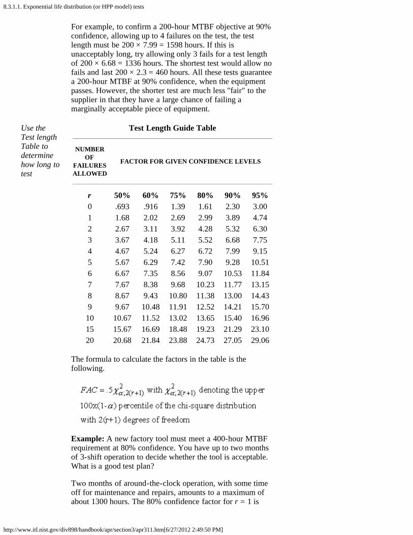
8.3.1.1. Exponential life distribution (or HPP model) tests
http://www.itl.nist.gov/div898/handbook/apr/section3/apr311.htm[6/27/2012 2:49:50 PM]
For example, to confirm a 200-hour MTBF objective at 90%confidence, allowing up to 4 failures on the test, the testlength must be 200 × 7.99 = 1598 hours. If this isunacceptably long, try allowing only 3 fails for a test lengthof 200 × 6.68 = 1336 hours. The shortest test would allow nofails and last 200 × 2.3 = 460 hours. All these tests guaranteea 200-hour MTBF at 90% confidence, when the equipmentpasses. However, the shorter test are much less "fair" to thesupplier in that they have a large chance of failing amarginally acceptable piece of equipment.
Use theTest lengthTable todeterminehow long totest
Test Length Guide Table
NUMBEROF
FAILURESALLOWED
FACTOR FOR GIVEN CONFIDENCE LEVELS
r 50% 60% 75% 80% 90% 95%0 .693 .916 1.39 1.61 2.30 3.001 1.68 2.02 2.69 2.99 3.89 4.742 2.67 3.11 3.92 4.28 5.32 6.303 3.67 4.18 5.11 5.52 6.68 7.754 4.67 5.24 6.27 6.72 7.99 9.155 5.67 6.29 7.42 7.90 9.28 10.516 6.67 7.35 8.56 9.07 10.53 11.847 7.67 8.38 9.68 10.23 11.77 13.158 8.67 9.43 10.80 11.38 13.00 14.439 9.67 10.48 11.91 12.52 14.21 15.7010 10.67 11.52 13.02 13.65 15.40 16.9615 15.67 16.69 18.48 19.23 21.29 23.1020 20.68 21.84 23.88 24.73 27.05 29.06
The formula to calculate the factors in the table is thefollowing.
Example: A new factory tool must meet a 400-hour MTBFrequirement at 80% confidence. You have up to two monthsof 3-shift operation to decide whether the tool is acceptable.What is a good test plan?
Two months of around-the-clock operation, with some timeoff for maintenance and repairs, amounts to a maximum ofabout 1300 hours. The 80% confidence factor for r = 1 is

8.3.1.1. Exponential life distribution (or HPP model) tests
http://www.itl.nist.gov/div898/handbook/apr/section3/apr311.htm[6/27/2012 2:49:50 PM]
2.99, so a test of 400 × 2.99 = about 1200 hours (with up to 1fail allowed) is the best that can be done.
Shortenrequiredtest timesby testingmore thanone system
NOTE: Exponential test times can be shortened significantlyif several similar tools or systems can be put on test at thesame time. Test time means the same as "tool hours" and onetool operating for 1000 hours is equivalent (as far as theexponential model is concerned) to 2 tools operating for 500hours each, or 10 tools operating for 100 hours each. Justcount all the fails from all the tools and the sum of the testhours from all the tools.

8.3.1.2. Lognormal or Weibull tests
http://www.itl.nist.gov/div898/handbook/apr/section3/apr312.htm[6/27/2012 2:49:51 PM]
8. Assessing Product Reliability 8.3. Reliability Data Collection 8.3.1. How do you plan a reliability assessment test?
8.3.1.2. Lognormal or Weibull tests
Planningreliabilitytests fordistributionsother thantheexponentialis difficultand involvesa lot ofguesswork
Planning a reliability test is not simple and straightforwardwhen the assumed model is lognormal or Weibull. Sincethese models have two parameters, no estimates are possiblewithout at least two test failures, and good estimates requireconsiderably more than that. Because of censoring, without agood guess ahead of time at what the unknown parametersare, any test plan may fail.
However, it is often possible to make a good guess ahead oftime about at least one of the unknown parameters -typically the "shape" parameter ( for the lognormal or for the Weibull). With one parameter assumed known, testplans can be derived that assure the reliability or failure rateof the product tested will be acceptable.
Lognormal Case (shape parameter known): Thelognormal model is used for many microelectronic wear-outfailure mechanisms, such as electromigration. As aproduction monitor, samples of microelectronic chips takenrandomly from production lots might be tested at levels ofvoltage and temperature that are high enough to significantlyaccelerate the occurrence of electromigration failures.Acceleration factors are known from previous testing andrange from several hundred to several thousand.
Lognormaltest plans,assumingsigma andtheaccelerationfactor areknown
The goal is to construct a test plan (put n units on stress testfor T hours and accept the lot if no more than r failuresoccur). The following assumptions are made:
The life distribution model is lognormalSigma = is known from past testing and does notvary appreciably from lot to lotLot reliability varies because T50's (the lognormalmedian or 50th percentile) differ from lot to lotThe acceleration factor from high stress to use stress isa known quantity "A"A stress time of T hours is practical as a line monitor
A nominal use T50 of Tu (combined with ) producesan acceptable use CDF (or use reliability function).This is equivalent to specifying an acceptable useCDF at, say, 100,000 hours to be a given value p and
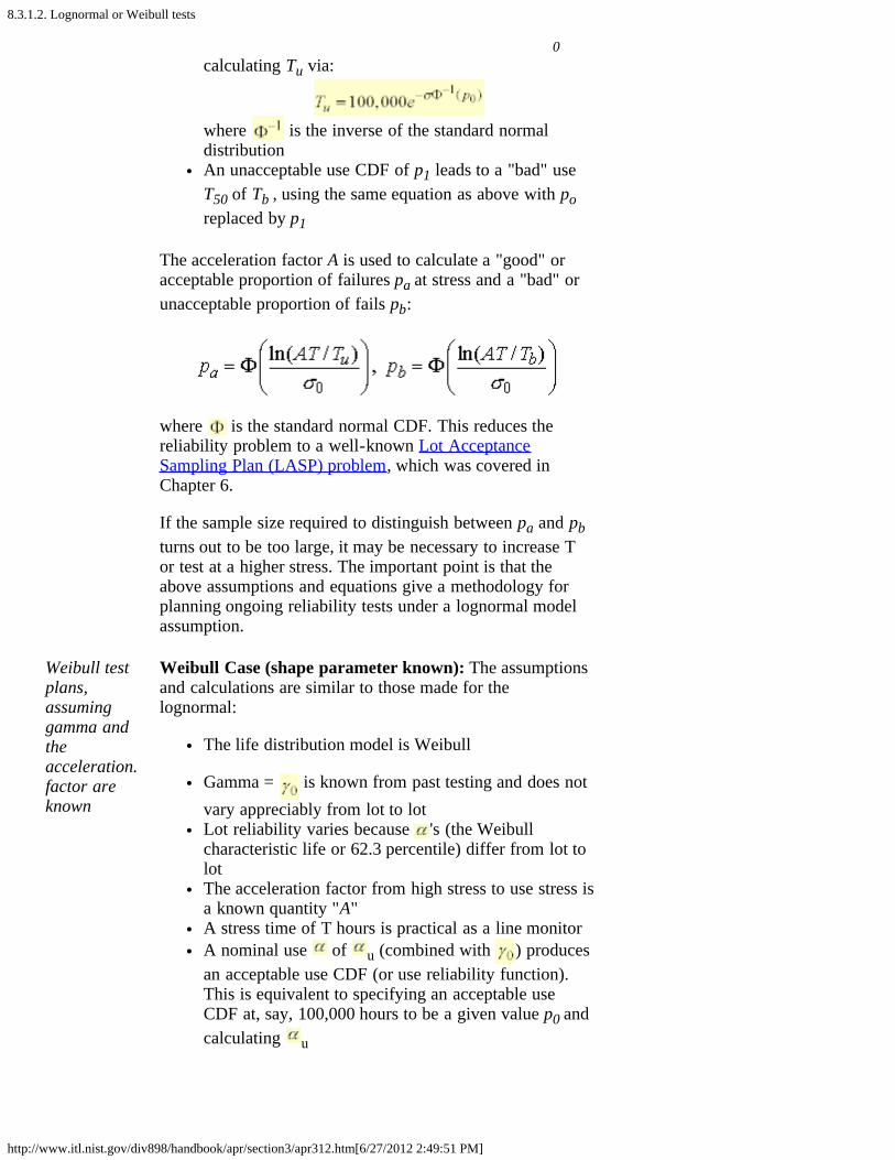
8.3.1.2. Lognormal or Weibull tests
http://www.itl.nist.gov/div898/handbook/apr/section3/apr312.htm[6/27/2012 2:49:51 PM]
0 calculating Tu via:
where is the inverse of the standard normaldistribution An unacceptable use CDF of p1 leads to a "bad" useT50 of Tb , using the same equation as above with poreplaced by p1
The acceleration factor A is used to calculate a "good" oracceptable proportion of failures pa at stress and a "bad" orunacceptable proportion of fails pb:
where is the standard normal CDF. This reduces thereliability problem to a well-known Lot AcceptanceSampling Plan (LASP) problem, which was covered inChapter 6.
If the sample size required to distinguish between pa and pbturns out to be too large, it may be necessary to increase Tor test at a higher stress. The important point is that theabove assumptions and equations give a methodology forplanning ongoing reliability tests under a lognormal modelassumption.
Weibull testplans,assuminggamma andtheacceleration.factor areknown
Weibull Case (shape parameter known): The assumptionsand calculations are similar to those made for thelognormal:
The life distribution model is Weibull
Gamma = is known from past testing and does notvary appreciably from lot to lotLot reliability varies because 's (the Weibullcharacteristic life or 62.3 percentile) differ from lot tolotThe acceleration factor from high stress to use stress isa known quantity "A"A stress time of T hours is practical as a line monitorA nominal use of u (combined with ) producesan acceptable use CDF (or use reliability function).This is equivalent to specifying an acceptable useCDF at, say, 100,000 hours to be a given value p0 andcalculating u
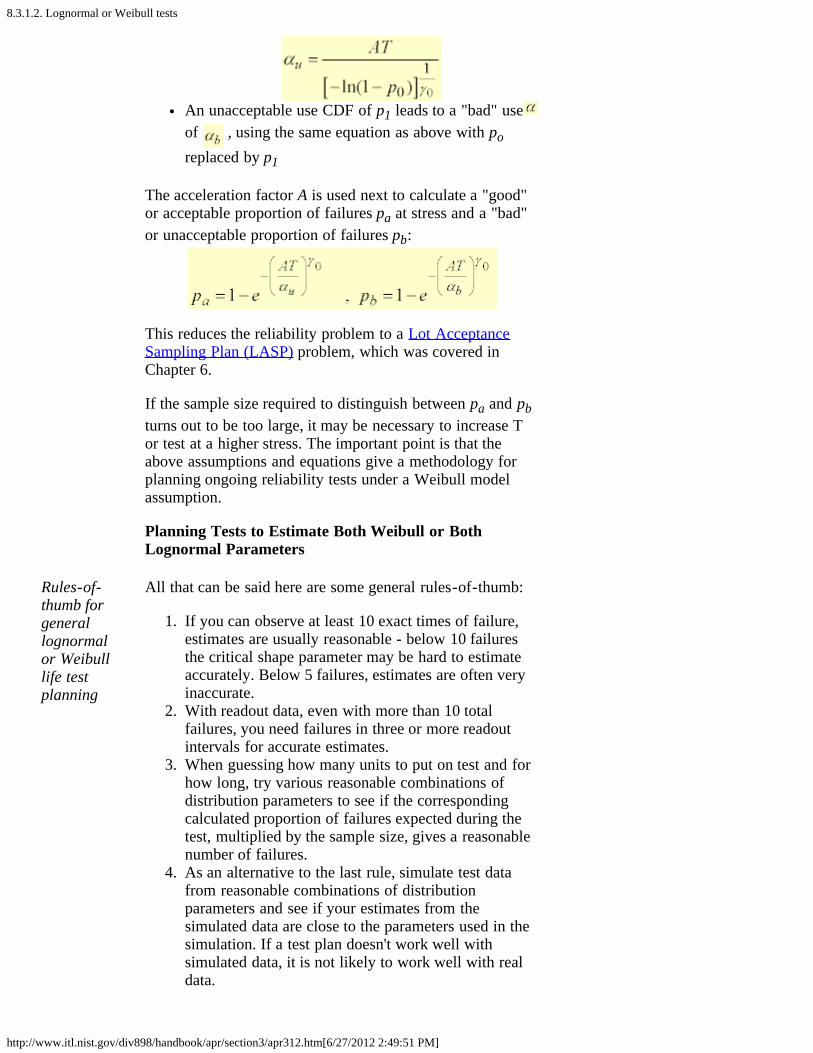
8.3.1.2. Lognormal or Weibull tests
http://www.itl.nist.gov/div898/handbook/apr/section3/apr312.htm[6/27/2012 2:49:51 PM]
An unacceptable use CDF of p1 leads to a "bad" useof , using the same equation as above with poreplaced by p1
The acceleration factor A is used next to calculate a "good"or acceptable proportion of failures pa at stress and a "bad"or unacceptable proportion of failures pb:
This reduces the reliability problem to a Lot AcceptanceSampling Plan (LASP) problem, which was covered inChapter 6.
If the sample size required to distinguish between pa and pbturns out to be too large, it may be necessary to increase Tor test at a higher stress. The important point is that theabove assumptions and equations give a methodology forplanning ongoing reliability tests under a Weibull modelassumption.
Planning Tests to Estimate Both Weibull or BothLognormal Parameters
Rules-of-thumb forgenerallognormalor Weibulllife testplanning
All that can be said here are some general rules-of-thumb:
1. If you can observe at least 10 exact times of failure,estimates are usually reasonable - below 10 failuresthe critical shape parameter may be hard to estimateaccurately. Below 5 failures, estimates are often veryinaccurate.
2. With readout data, even with more than 10 totalfailures, you need failures in three or more readoutintervals for accurate estimates.
3. When guessing how many units to put on test and forhow long, try various reasonable combinations ofdistribution parameters to see if the correspondingcalculated proportion of failures expected during thetest, multiplied by the sample size, gives a reasonablenumber of failures.
4. As an alternative to the last rule, simulate test datafrom reasonable combinations of distributionparameters and see if your estimates from thesimulated data are close to the parameters used in thesimulation. If a test plan doesn't work well withsimulated data, it is not likely to work well with realdata.

8.3.1.2. Lognormal or Weibull tests
http://www.itl.nist.gov/div898/handbook/apr/section3/apr312.htm[6/27/2012 2:49:51 PM]
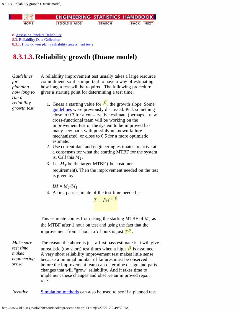
8.3.1.3. Reliability growth (Duane model)
http://www.itl.nist.gov/div898/handbook/apr/section3/apr313.htm[6/27/2012 2:49:52 PM]
8. Assessing Product Reliability 8.3. Reliability Data Collection 8.3.1. How do you plan a reliability assessment test?
8.3.1.3. Reliability growth (Duane model)
Guidelinesforplanninghow long torun areliabilitygrowth test
A reliability improvement test usually takes a large resourcecommitment, so it is important to have a way of estimatinghow long a test will be required. The following proceduregives a starting point for determining a test time:
1. Guess a starting value for , the growth slope. Someguidelines were previously discussed. Pick somethingclose to 0.3 for a conservative estimate (perhaps a newcross-functional team will be working on theimprovement test or the system to be improved hasmany new parts with possibly unknown failuremechanisms), or close to 0.5 for a more optimisticestimate.
2. Use current data and engineering estimates to arrive ata consensus for what the starting MTBF for the systemis. Call this M1.
3. Let MT be the target MTBF (the customerrequirement). Then the improvement needed on the testis given by
IM = MT/M14. A first pass estimate of the test time needed is
This estimate comes from using the starting MTBF of M1 asthe MTBF after 1 hour on test and using the fact that theimprovement from 1 hour to T hours is just .
Make suretest timemakesengineeringsense
The reason the above is just a first pass estimate is it will giveunrealistic (too short) test times when a high is assumed.A very short reliability improvement test makes little sensebecause a minimal number of failures must be observedbefore the improvement team can determine design and partschanges that will "grow" reliability. And it takes time toimplement these changes and observe an improved repairrate.
Iterative Simulation methods can also be used to see if a planned test

8.3.1.3. Reliability growth (Duane model)
http://www.itl.nist.gov/div898/handbook/apr/section3/apr313.htm[6/27/2012 2:49:52 PM]
simulationis an aidfor testplanning
is likely to generate data that will demonstrate an assumedgrowth rate.

8.3.1.4. Accelerated life tests
http://www.itl.nist.gov/div898/handbook/apr/section3/apr314.htm[6/27/2012 2:49:53 PM]
8. Assessing Product Reliability 8.3. Reliability Data Collection 8.3.1. How do you plan a reliability assessment test?
8.3.1.4. Accelerated life tests
Acceleratedtesting isneeded whentesting evenlarge samplesizes at usestress wouldyield few orno failureswithin areasonabletime
Accelerated life tests are component life tests withcomponents operated at high stresses and failure dataobserved. While high stress testing can be performed for thesole purpose of seeing where and how failures occur andusing that information to improve component designs ormake better component selections, we will focus in thissection on accelerated life testing for the following twopurposes:
1. To study how failure is accelerated by stress and fit anacceleration model to data from multiple stress cells
2. To obtain enough failure data at high stress toaccurately project (extrapolate) what the CDF at usewill be.
If we already know the acceleration model (or theacceleration factor to typical use conditions from high stresstest conditions), then the methods described two pages agocan be used. We assume, therefore, that the accelerationmodel is not known in advance.
Testplanningmeanspickingstress levelsand samplesizes andtest times toproduceenough datato fit modelsand makeprojections
Test planning and operation for a (multiple) stress cell lifetest experiment consists of the following:
Pick several combinations of the relevant stresses (thestresses that accelerate the failure mechanism underinvestigation). Each combination is a "stress cell".Note that you are planning for only one mechanism offailure at a time. Failures on test due to any othermechanism will be considered censored run times.Make sure stress levels used are not too high - to thepoint where new failure mechanisms that would neveroccur at use stress are introduced. Picking a maximumallowable stress level requires experience and/or goodengineering judgment.Put random samples of components in each stress celland run the components in each cell for fixed (butpossibly different) lengths of time.Gather the failure data from each cell and use the datato fit an acceleration model and a life distributionmodel and use these models to project reliability atuse stress conditions.

8.3.1.4. Accelerated life tests
http://www.itl.nist.gov/div898/handbook/apr/section3/apr314.htm[6/27/2012 2:49:53 PM]
Test planning would be similar to topics already covered inthe chapters that discussed modeling and experimentaldesign except for one important point. When you testcomponents in a stress cell for a fixed length test, it istypical that some (or possibly many) of the components endthe test without failing. This is the censoring problem, and itgreatly complicates experimental design to the point atwhich it becomes almost as much of an art (based onengineering judgment) as a statistical science.
An example will help illustrate the design issues. Assume ametal migration failure mode is believed to follow the 2-stress temperature voltage model given by
Normal use conditions are 4 volts and 25 degrees Celsius,and the high stress levels under consideration are 6, 8,12volts and 85o, 105o and 125o. It probably would be a wasteof resources to test at (6v, 85o), or even possibly (8v, 85o)or (6v,105o) since these cells are not likely to have enoughstress acceleration to yield a reasonable number of failureswithin typical test times.
If you write all the 9 possible stress cell combinations in a3x3 matrix with voltage increasing by rows and temperatureincreasing by columns, the result would look like the matrixbelow:
Matrix Leading to "Backward L Design"
6v, 85o 6v, 105o 6v, 125o
8v, 85o 8v,105o 8v,125o
12v,85o 12v,105o 12v,125o
"BackwardsL" designsare commoninacceleratedlife testing.Put moreexperimentalunits inlower stresscells.
The combinations in bold are the most likely design choicescovering the full range of both stresses, but still hopefullyhaving enough acceleration to produce failures. This is theso-called "backwards L" design commonly used foracceleration modeling experiments.
Note: It is good design practice to put more of your testunits in the lower stress cells, to make up for the fact thatthese cells will have a smaller proportion of units failing.

8.3.1.4. Accelerated life tests
http://www.itl.nist.gov/div898/handbook/apr/section3/apr314.htm[6/27/2012 2:49:53 PM]
Sometimessimulation isthe best wayto learnwhether atest plan hasa chance ofworking
Design by Simulation:
A lengthy, but better way to choose a test matrix is thefollowing:
Pick an acceleration model and a life distributionmodel (as usual).Guess at the shape parameter value of the lifedistribution model based on literature studies or earlierexperiments. The shape parameter should remain thesame for all stress cells. Choose a scale parametervalue at use so that the use stress CDF exactly meetsrequirements (i.e., for the lognormal, pick a use T50that gives the desired use reliability - for a Weibullmodel choice, do the same for the characteristic lifeparameter).Guess at the acceleration model parameters values (H and , for the 2-stress model shown above). Again,use whatever is in the literature for similar failuremechanisms or data from earlier experiments).Calculate acceleration factors from any proposed testcells to use stress and divide the use scale parameterby these acceleration factors to obtain "trial" cell scaleparameters.Simulate cell data for each proposed stress cell usingthe derived cell scale parameters and the guessedshape parameter.Check that every proposed cell has sufficient failuresto give good estimates. Adjust the choice of stress cells and the sample sizeallocations until you are satisfied that, if everythinggoes as expected, the experiment will yield enoughdata to provide good estimates of the modelparameters.
After youmakeadvanceestimates, itis sometimespossible toconstruct anoptimalexperimentaldesign - butsoftware forthis isscarce
Optimal Designs:
Recent work on designing accelerated life tests has shown itis possible, for a given choice of models and assumed valuesof the unknown parameters, to construct an optimal design(one which will have the best chance of providing goodsample estimates of the model parameters). These optimaldesigns typically select stress levels as far apart as possibleand heavily weight the allocation of sample units to thelower stress cells. However, unless the experimenter can findsoftware that incorporates these optimal methods for his orher particular choice of models, the methods describedabove are the most practical way of designing accelerationexperiments.

8.3.1.5. Bayesian gamma prior model
http://www.itl.nist.gov/div898/handbook/apr/section3/apr315.htm[6/27/2012 2:49:54 PM]
8. Assessing Product Reliability 8.3. Reliability Data Collection 8.3.1. How do you plan a reliability assessment test?
8.3.1.5. Bayesian gamma prior model
How toplan aBayesiantest toconfirm asystemmeets itsMTBFobjective
Review Bayesian Basics and assumptions, if needed. We startat the point when gamma prior parameters a and b havealready been determined. Assume we have a given MTBFobjective, M, and a desired confidence level of 100×(1- α).We want to confirm the system will have an MTBF of at leastM at the 100×(1- α) confidence level. As in the section onclassical (HPP) test plans, we pick a number of failures, r, thatwe can allow on the test. We need a test time T such that wecan observe up to r failures and still "pass" the test. If the testtime is too long (or too short), we can iterate with a differentchoice of r.
When the test ends, the posterior gamma distribution will have(worst case - assuming exactly r failures) new parameters of
a' = a + r, b' = b + T
and passing the test means that the failure rate λ1- α, the upper100×(1- α) percentile for the posterior gamma, has to equalthe target failure rate 1/M. But this percentile is, by definition,G -1(1- α; a', b'), with G -1 denoting the inverse of the gammadistribution with parameters a', b'. We can find the value of Tthat satisfies G -1(1- α; a', b') = 1/M by trial and error.However, based on the properties of the gamma distribution, itturns out that we can calculate T directly by using
T = M×(G -1(1- α; a', 1)) - b
Special Case: The Prior Has a = 1 (The "Weak" Prior)
When theprior is aweak priorwith a = 1,theBayesiantest isalwaysshorterthan theclassical
There is a very simple way to calculate the required Bayesiantest time when the prior is a weak prior with a = 1. Just usethe Test Length Guide Table to calculate the classical testtime. Call this Tc. The Bayesian test time T is just Tc minusthe prior parameter b (i.e., T = Tc - b). If the b parameter wasset equal to (ln 2) × MTBF50 (where MTBF50 is the consensuschoice for an "even money" MTBF), then
T = Tc - (ln 2) × MTBF50
This shows that when a weak prior is used, the Bayesian test
8.3.1.5. Bayesian gamma prior model
http://www.itl.nist.gov/div898/handbook/apr/section3/apr315.htm[6/27/2012 2:49:54 PM]
test time is always less than the corresponding classical test time.That is why this prior is also known as a friendly prior.
Note: In general, Bayesian test times can be shorter, or longer,than the corresponding classical test times, depending on thechoice of prior parameters. However, the Bayesian time willalways be shorter when the prior parameter a is less than, orequal to, 1.
Example: Calculating a Bayesian Test Time
Example A new piece of equipment has to meet a MTBF requirementof 500 hours at 80 % confidence. A group of engineers decideto use their collective experience to determine a Bayesiangamma prior using the 50/95 method described in Section 2.They think 600 hours is a likely MTBF value and they arevery confident that the MTBF will exceed 250. Following theexample in Section 2, they determine that the gamma priorparameters are a = 2.863 and b = 1522.46.
Now they want to determine an appropriate test time so thatthey can confirm a MTBF of 500 with at least 80 %confidence, provided they have no more than two failures.
We obtain a test time of 1756.117 hours using
500×(G -1(1-0.2; 2.863+2, 1)) - 1522.46
To compare this result to the classical test time required, usethe Test Length Guide Table. The table factor is 4.28, so thetest time needed is 500 × 4.28 = 2140 hours for a non-Bayesian test. The Bayesian test saves about 384 hours, or an18 % savings. If the test is run for 1756 hours, with no morethan two failures, then an MTBF of at least 500 hours hasbeen confirmed at 80 % confidence.
If, instead, the engineers had decided to use a weak prior withan MTBF50 of 600, the required test time would have been
2140 - 600 × ln 2 = 1724 hours

8.4. Reliability Data Analysis
http://www.itl.nist.gov/div898/handbook/apr/section4/apr4.htm[6/27/2012 2:49:55 PM]
8. Assessing Product Reliability
8.4. Reliability Data Analysis
After you have obtained component or system reliability data,how do you fit life distribution models, reliability growthmodels, or acceleration models? How do you estimate failurerates or MTBF's and project component or system reliabilityat use conditions? This section answers these kinds ofquestions.
Detailedoutline forSection 4
The detailed outline for section 4 follows.
4. Reliability Data Analysis
1. How do you estimate life distribution parameters fromcensored data?
1. Graphical estimation 2. Maximum Likelihood Estimation (MLE) 3. A Weibull MLE example
2. How do you fit an acceleration model? 1. Graphical estimation 2. Maximum likelihood3. Fitting models using degradation data instead of
failures 3. How do you project reliability at use conditions? 4. How do you compare reliability between two or more
populations? 5. How do you fit system repair rate models?
1. Constant repair rate (HPP/Exponential) model2. Power law (Duane) model 3. Exponential law model
6. How do you estimate reliability using the Bayesiangamma prior model?

8.4.1. How do you estimate life distribution parameters from censored data?
http://www.itl.nist.gov/div898/handbook/apr/section4/apr41.htm[6/27/2012 2:49:55 PM]
8. Assessing Product Reliability 8.4. Reliability Data Analysis
8.4.1. How do you estimate life distributionparameters from censored data?
Graphicalestimationmethods(aided bycomputerline fits)are easyand quick
Maximumlikelihoodmethodsareusuallymoreprecise -butrequirespecialsoftware
Two widely used general methods will be described in thissection:
Graphical estimationMaximum Likelihood Estimation (MLE)
Recommendation On Which Method to Use
Maximum likelihood estimation (except when the failure dataare very sparse - i.e., only a few failures) is a more precise andflexible method. However, with censored data, the method ofmaximum likelihood estimation requires special computerprograms for distributions other than the exponential. This isno longer an obstacle since, in recent years, many statisticalsoftware packages have added reliability platforms that willcalculate MLE's and most of these packages will estimateacceleration model parameters and give confidence bounds aswell.
If important business decisions are based on reliabilityprojections made from life test data and accelerationmodeling, then it pays to obtain state-of-the art MLEreliability software. Otherwise, for monitoring and trackingreliability, estimation methods based on computer-augmentedgraphical procedures will often suffice.

8.4.1.1. Graphical estimation
http://www.itl.nist.gov/div898/handbook/apr/section4/apr411.htm[6/27/2012 2:49:56 PM]
8. Assessing Product Reliability 8.4. Reliability Data Analysis 8.4.1. How do you estimate life distribution parameters from censored data?
8.4.1.1. Graphical estimation
The line on aprobabilityplot uniquelyidentifiesdistributionalparameters
Once you have calculated plotting positions from yourfailure data, and have generated the probability plot for yourchosen model, parameter estimation follows easily. Butalong with the mechanics of graphical estimation, be awareof both the advantages and the disadvantages of graphicalestimation methods.
Mostprobabilityplots havesimpleproceduresto calculateunderlyingdistributionparameterestimates
Graphical Estimation Mechanics:
If you draw a line through points on a probability plot, thereare usually simple rules to find estimates of the slope (orshape parameter) and the scale parameter. On lognormalprobability plot with time on the x-axis and cumulativepercent on the y-axis, draw horizontal lines from the 34thand the 50th percentiles across to the fitted line, and dropvertical lines to the time axis from these intersection points.The time corresponding to the 50th percentile is the T50estimate. Divide T50 by the time corresponding to the 34thpercentile (this is called T34). The natural logarithm of thatratio is the estimate of sigma, or the slope of the line (σ =ln(T50 / T34)).
For a Weibull probability plot draw a horizontal line fromthe y-axis to the fitted line at the 62.3 percentile point. Thatestimation line intersects the line through the points at atime that is the estimate of the characteristic life parameterα. In order to estimate the slope of the fitted line (or theshape parameter γ), choose any two points on the fitted lineand divide the change in the y variable by the change in xvariable.
Using acomputergeneratedline fittingroutineremovessubjectivityand can leaddirectly tocomputer
To remove the subjectivity of drawing a line through thepoints, a least-squares (regression) fit can be performedusing the equations described in the section on probabilityplotting. An example of this for the Weibull was also shownin that section. Another example of a Weibull plot for thesame data appears later in this section.
Finally, if you have exact times and complete samples (nocensoring), many software packages have built-inProbability Plotting functions. Examples were shown in the

8.4.1.1. Graphical estimation
http://www.itl.nist.gov/div898/handbook/apr/section4/apr411.htm[6/27/2012 2:49:56 PM]
parameterestimatesbased on theplottingpositions
sections describing various life distribution models.
Doprobabilityplots even ifyou use someother methodfor the finalestimates
Advantages of Graphical Methods of Estimation:
Graphical methods are quick and easy to use andmake visual sense.Calculations can be done with little or no specialsoftware needed.Visual test of model (i.e., how well the points line up)is an additional benefit.
Disadvantages of Graphical Methods of Estimation
Perhaps theworstdrawback ofgraphicalestimation isyou cannotget legitimateconfidenceintervals forthe estimates
The statistical properties of graphical estimates (i.e., howprecise are they on average) are not good:
they are biased,even with large samples, they are not minimumvariance (i.e., most precise) estimates,graphical methods do not give confidence intervalsfor the parameters (intervals generated by a regressionprogram for this kind of data are incorrect), andformal statistical tests about model fit or parametervalues cannot be performed with graphical methods.
As we will see in the next section, Maximum LikelihoodEstimates overcome all these disadvantages - at least forreliability data sets with a reasonably large number offailures - at a cost of losing all the advantages listed abovefor graphical estimation.

8.4.1.2. Maximum likelihood estimation
http://www.itl.nist.gov/div898/handbook/apr/section4/apr412.htm[6/27/2012 2:49:57 PM]
8. Assessing Product Reliability 8.4. Reliability Data Analysis 8.4.1. How do you estimate life distribution parameters from censored data?
8.4.1.2. Maximum likelihood estimation
There isnothingvisualabout themaximumlikelihoodmethod -but it is apowerfulmethodand, atleast forlargesamples,veryprecise
Maximum likelihood estimation begins with writing amathematical expression known as the Likelihood Functionof the sample data. Loosely speaking, the likelihood of a setof data is the probability of obtaining that particular set ofdata, given the chosen probability distribution model. Thisexpression contains the unknown model parameters. Thevalues of these parameters that maximize the samplelikelihood are known as the Maximum Likelihood Estimatesor MLE's.
Maximum likelihood estimation is a totally analyticmaximization procedure. It applies to every form of censoredor multicensored data, and it is even possible to use thetechnique across several stress cells and estimate accelerationmodel parameters at the same time as life distributionparameters. Moreover, MLE's and Likelihood Functionsgenerally have very desirable large sample properties:
they become unbiased minimum variance estimators asthe sample size increasesthey have approximate normal distributions andapproximate sample variances that can be calculatedand used to generate confidence boundslikelihood functions can be used to test hypothesesabout models and parameters
With smallsamples,MLE's maynot be veryprecise andmay evengenerate aline thatlies aboveor belowthe datapoints
There are only two drawbacks to MLE's, but they areimportant ones:
With small numbers of failures (less than 5, andsometimes less than 10 is small), MLE's can be heavilybiased and the large sample optimality properties do notapplyCalculating MLE's often requires specialized softwarefor solving complex non-linear equations. This is lessof a problem as time goes by, as more statisticalpackages are upgrading to contain MLE analysiscapability every year.
Additional information about maximum likelihoodestimatation can be found in Chapter 1.
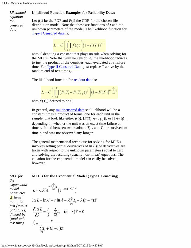
8.4.1.2. Maximum likelihood estimation
http://www.itl.nist.gov/div898/handbook/apr/section4/apr412.htm[6/27/2012 2:49:57 PM]
Likelihoodequationforcensoreddata
Likelihood Function Examples for Reliability Data:
Let f(t) be the PDF and F(t) the CDF for the chosen lifedistribution model. Note that these are functions of t and theunknown parameters of the model. The likelihood function forType I Censored data is:
with C denoting a constant that plays no role when solving forthe MLE's. Note that with no censoring, the likelihood reducesto just the product of the densities, each evaluated at a failuretime. For Type II Censored Data, just replace T above by therandom end of test time tr.
The likelihood function for readout data is:
with F(T0) defined to be 0.
In general, any multicensored data set likelihood will be aconstant times a product of terms, one for each unit in thesample, that look like either f(ti), [F(Ti)-F(Ti-1)], or [1-F(ti)],depending on whether the unit was an exact time failure attime ti, failed between two readouts Ti-1 and Ti, or survived totime ti and was not observed any longer.
The general mathematical technique for solving for MLE'sinvolves setting partial derivatives of ln L (the derivatives aretaken with respect to the unknown parameters) equal to zeroand solving the resulting (usually non-linear) equations. Theequation for the exponential model can easily be solved,however.
MLE fortheexponentialmodelparameter
turnsout to bejust (total #of failures)divided by(total unittest time)
MLE's for the Exponential Model (Type I Censoring):

8.4.1.2. Maximum likelihood estimation
http://www.itl.nist.gov/div898/handbook/apr/section4/apr412.htm[6/27/2012 2:49:57 PM]
Note: The MLE of the failure rate (or repair rate) in theexponential case turns out to be the total number of failuresobserved divided by the total unit test time. For the MLE ofthe MTBF, take the reciprocal of this or use the total unit testhours divided by the total observed failures.
There are examples of Weibull and lognormal MLE analysislater in this section.

8.4.1.3. A Weibull maximum likelihood estimation example
http://www.itl.nist.gov/div898/handbook/apr/section4/apr413.htm[6/27/2012 2:49:58 PM]
8. Assessing Product Reliability 8.4. Reliability Data Analysis 8.4.1. How do you estimate life distribution parameters from censored data?
8.4.1.3. A Weibull maximum likelihood estimationexample
ReliabilityanalysisusingWeibulldata
We will plot Weibull censored data and estimate parameters using datafrom a previous example (8.2.2.1).
The recorded failure times were 54, 187, 216, 240, 244, 335, 361, 373,375, and 386 hours, and 10 units that did not fail were removed from thetest at 500 hours. The data are summarized in the following table.
Time Censored Frequency 54 0 1 187 0 1 216 0 1 240 0 1 244 0 1 335 0 1 361 0 1 373 0 1 375 0 1 386 0 1 500 1 10
The column labeled "Time" contains failure and censoring times, the"Censored" column contains a variable to indicate whether the time incolumn one is a failure time or a censoring time, and the "Frequency"column shows how many units failed or were censored at that time.
First, we generate a survival curve using the Kaplan-Meier method and aWeibull probability plot. Note: Some software packages might use thename "Product Limit Method" or "Product Limit Survival Estimates"instead of the equivalent name "Kaplan-Meier".
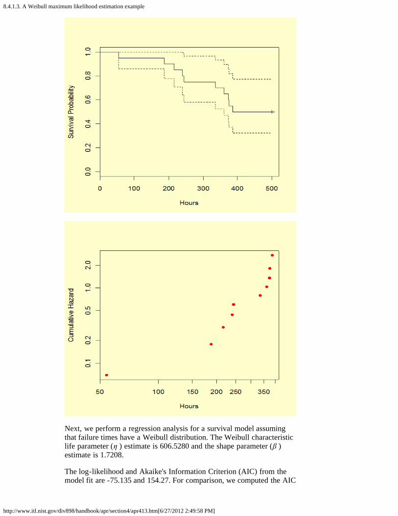
8.4.1.3. A Weibull maximum likelihood estimation example
http://www.itl.nist.gov/div898/handbook/apr/section4/apr413.htm[6/27/2012 2:49:58 PM]
Next, we perform a regression analysis for a survival model assumingthat failure times have a Weibull distribution. The Weibull characteristiclife parameter (η ) estimate is 606.5280 and the shape parameter (β )estimate is 1.7208.
The log-likelihood and Akaike's Information Criterion (AIC) from themodel fit are -75.135 and 154.27. For comparison, we computed the AIC
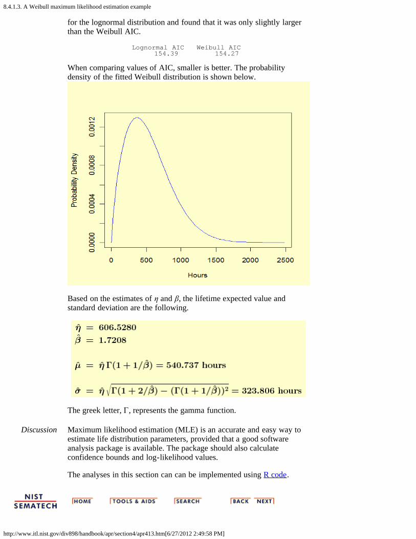
8.4.1.3. A Weibull maximum likelihood estimation example
http://www.itl.nist.gov/div898/handbook/apr/section4/apr413.htm[6/27/2012 2:49:58 PM]
for the lognormal distribution and found that it was only slightly largerthan the Weibull AIC.
Lognormal AIC Weibull AIC 154.39 154.27
When comparing values of AIC, smaller is better. The probabilitydensity of the fitted Weibull distribution is shown below.
Based on the estimates of η and β, the lifetime expected value andstandard deviation are the following.
The greek letter, Γ, represents the gamma function.
Discussion Maximum likelihood estimation (MLE) is an accurate and easy way toestimate life distribution parameters, provided that a good softwareanalysis package is available. The package should also calculateconfidence bounds and log-likelihood values.
The analyses in this section can can be implemented using R code.

8.4.2. How do you fit an acceleration model?
http://www.itl.nist.gov/div898/handbook/apr/section4/apr42.htm[6/27/2012 2:49:59 PM]
8. Assessing Product Reliability 8.4. Reliability Data Analysis
8.4.2. How do you fit an acceleration model?
Accelerationmodels canbe fit byeithergraphicalproceduresor maximumlikelihoodmethods
As with estimating life distribution model parameters, thereare two general approaches for estimating acceleration modelparameters:
Graphical estimation (or computer procedures basedon a graphical approach)Maximum Likelihood Estimation (an analyticapproach based on writing the likelihood of all the dataacross all the cells, incorporating the accelerationmodel).
The same comments and recommendations concerning thesemethods still apply. Note that it is even harder, however, tofind useful software programs that will do maximumlikelihood estimation across stress cells and fit and testacceleration models.
Sometimes itis possibleto fit amodel usingdegradationdata
Another promising method of fitting acceleration models issometimes possible when studying failure mechanismscharacterized by a stress-induced gradual degradationprocess that causes the eventual failure. This approach fitsmodels based on degradation data and has the advantage ofnot actually needing failures. This overcomes censoringlimitations by providing measurement data at consecutivetime intervals for every unit in every stress cell.
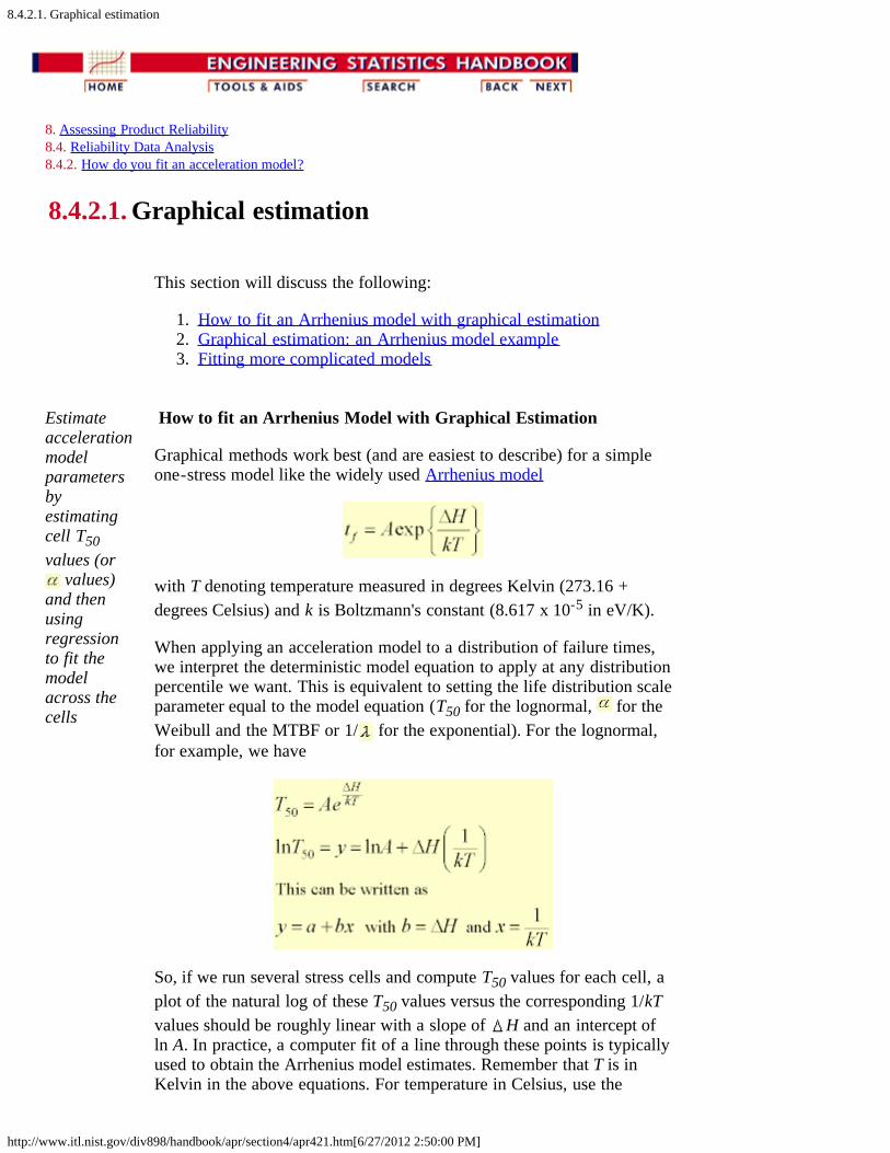
8.4.2.1. Graphical estimation
http://www.itl.nist.gov/div898/handbook/apr/section4/apr421.htm[6/27/2012 2:50:00 PM]
8. Assessing Product Reliability 8.4. Reliability Data Analysis 8.4.2. How do you fit an acceleration model?
8.4.2.1. Graphical estimation
This section will discuss the following:
1. How to fit an Arrhenius model with graphical estimation2. Graphical estimation: an Arrhenius model example3. Fitting more complicated models
Estimateaccelerationmodelparametersbyestimatingcell T50values (or
values)and thenusingregressionto fit themodelacross thecells
How to fit an Arrhenius Model with Graphical Estimation
Graphical methods work best (and are easiest to describe) for a simpleone-stress model like the widely used Arrhenius model
with T denoting temperature measured in degrees Kelvin (273.16 +degrees Celsius) and k is Boltzmann's constant (8.617 x 10⁻⁵ in eV/K).
When applying an acceleration model to a distribution of failure times,we interpret the deterministic model equation to apply at any distributionpercentile we want. This is equivalent to setting the life distribution scaleparameter equal to the model equation (T50 for the lognormal, for theWeibull and the MTBF or 1/ for the exponential). For the lognormal,for example, we have
So, if we run several stress cells and compute T50 values for each cell, aplot of the natural log of these T50 values versus the corresponding 1/kTvalues should be roughly linear with a slope of H and an intercept ofln A. In practice, a computer fit of a line through these points is typicallyused to obtain the Arrhenius model estimates. Remember that T is inKelvin in the above equations. For temperature in Celsius, use the

8.4.2.1. Graphical estimation
http://www.itl.nist.gov/div898/handbook/apr/section4/apr421.htm[6/27/2012 2:50:00 PM]
following for 1/kT:11605/(t °C + 273.16).
An example will illustrate the procedure.
Graphical Estimation: An Arrhenius Model Example:
Arrheniusmodelexample
Component life tests were run at three temperatures: 85 °C, 105 °C and 125 °C. The lowest temperature cell was populated with 100components; the 105 °C cell had 50 components and the highest stresscell had 25 components. All tests were run until either all the units in thecell had failed or 1000 hours was reached. Acceleration was assumed tofollow an Arrhenius model and the life distribution model for the failuremode was believed to be lognormal. The normal operating temperaturefor the components is 25 °C and it is desired to project the use CDF at100,000 hours.
Test results:
Cell 1 (85 °C): 5 failures at 401, 428, 695, 725 and 738 hours. Ninety-five units were censored at 1000 hours running time.
Cell 2 (105 °C): 35 failures at 171, 187, 189, 266, 275, 285, 301, 302,305, 316, 317, 324, 349, 350, 386, 405, 480, 493, 530, 534, 536, 567,589, 598, 599, 614, 620, 650, 668, 685, 718, 795, 854, 917, and 926hours. Fifteen units were censored at 1000 hours running time.
Cell 3 (125 °C): 24 failures at 24, 42, 92, 93, 141, 142, 143, 159, 181,188, 194, 199, 207, 213, 243, 256, 259, 290, 294, 305, 392, 454, 502 and696. One unit was censored at 1000 hours running time.
Failure analysis confirmed that all failures were due to the same failuremechanism (if any failures due to another mechanism had occurred, theywould have been considered censored run times in the Arrheniusanalysis).
Steps to Fitting the Distribution Model and the Arrhenius Model:
Do plots for each cell and estimate T50 and sigma as previouslydiscussed.Plot all the cells on the same graph and check whether the lines areroughly parallel (a necessary consequence of true acceleration).If probability plots indicate that the lognormal model is appropriateand that sigma is consistant among cells, plot ln T50 versus 11605/(t °C + 273.16) for each cell, check for linearity and fit astraight line through the points. Since the points have differentvalues of precision, due to different numbers of failures in eachcell, it is recommended that the number of failures in each cell beused as weights in a regression when fitting a line through thepoints.Use the slope of the line as the H estimate and calculate theArrhenius A constant from the intercept using A = eintercept.Estimate the common sigma across all the cells by the weightedaverage of the individual cell sigma estimates. Use the number of
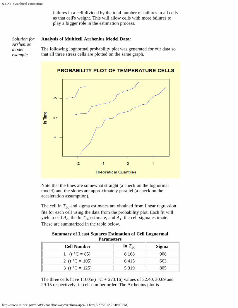
8.4.2.1. Graphical estimation
http://www.itl.nist.gov/div898/handbook/apr/section4/apr421.htm[6/27/2012 2:50:00 PM]
failures in a cell divided by the total number of failures in all cellsas that cell's weight. This will allow cells with more failures toplay a bigger role in the estimation process.
Solution forArrheniusmodelexample
Analysis of Multicell Arrhenius Model Data:
The following lognormal probability plot was generated for our data sothat all three stress cells are plotted on the same graph.
Note that the lines are somewhat straight (a check on the lognormalmodel) and the slopes are approximately parallel (a check on theacceleration assumption).
The cell ln T50 and sigma estimates are obtained from linear regressionfits for each cell using the data from the probability plot. Each fit willyield a cell Ao, the ln T50 estimate, and A1, the cell sigma estimate.These are summarized in the table below.
Summary of Least Squares Estimation of Cell LognormalParameters
Cell Number ln T50 Sigma1 (t °C = 85) 8.168 .9082 (t °C = 105) 6.415 .6633 (t °C = 125) 5.319 .805
The three cells have 11605/(t °C + 273.16) values of 32.40, 30.69 and29.15 respectively, in cell number order. The Arrhenius plot is
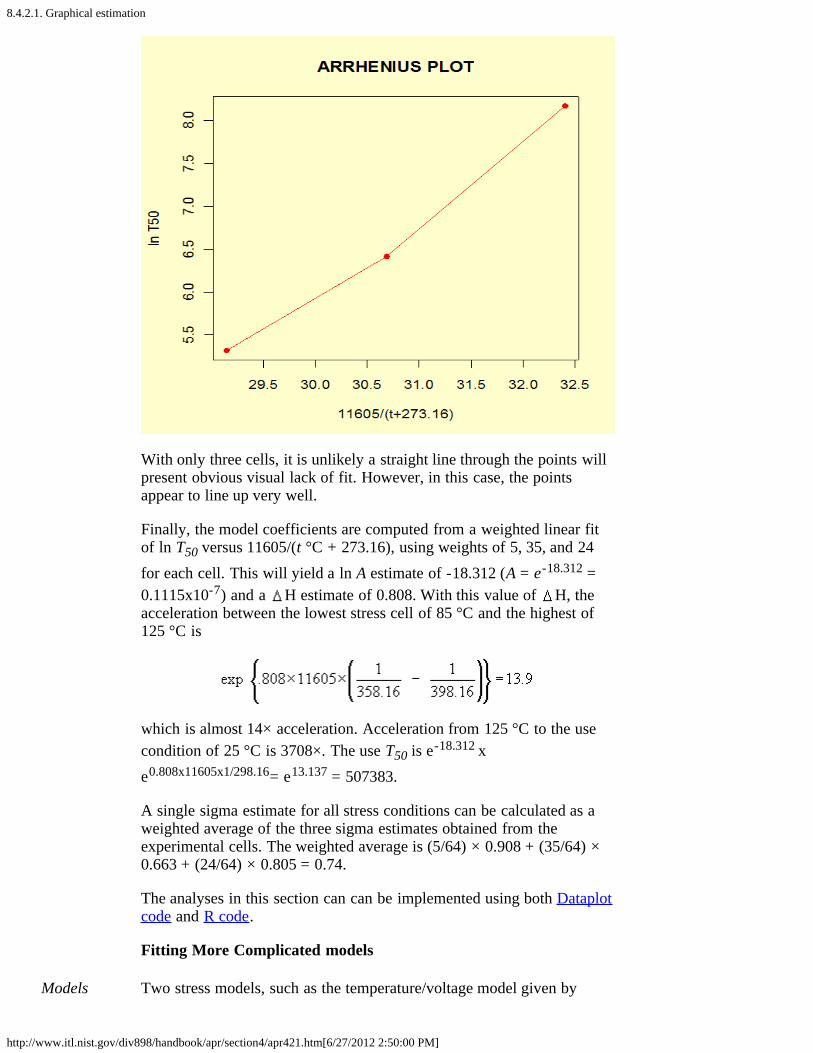
8.4.2.1. Graphical estimation
http://www.itl.nist.gov/div898/handbook/apr/section4/apr421.htm[6/27/2012 2:50:00 PM]
With only three cells, it is unlikely a straight line through the points willpresent obvious visual lack of fit. However, in this case, the pointsappear to line up very well.
Finally, the model coefficients are computed from a weighted linear fitof ln T50 versus 11605/(t °C + 273.16), using weights of 5, 35, and 24for each cell. This will yield a ln A estimate of -18.312 (A = e-18.312 =0.1115x10⁻⁷) and a H estimate of 0.808. With this value of H, theacceleration between the lowest stress cell of 85 °C and the highest of125 °C is
which is almost 14× acceleration. Acceleration from 125 °C to the usecondition of 25 °C is 3708×. The use T50 is e-18.312 xe0.808x11605x1/298.16= e13.137 = 507383.
A single sigma estimate for all stress conditions can be calculated as aweighted average of the three sigma estimates obtained from theexperimental cells. The weighted average is (5/64) × 0.908 + (35/64) ×0.663 + (24/64) × 0.805 = 0.74.
The analyses in this section can can be implemented using both Dataplotcode and R code.
Fitting More Complicated models
Models Two stress models, such as the temperature/voltage model given by

8.4.2.1. Graphical estimation
http://www.itl.nist.gov/div898/handbook/apr/section4/apr421.htm[6/27/2012 2:50:00 PM]
involvingseveralstresses canbe fit usingmultipleregression need at least four or five carefully chosen stress cells to estimate all the
parameters. The Backwards L design previously described is an exampleof a design for this model. The bottom row of the "backward L" could beused for a plot testing the Arrhenius temperature dependence, similar tothe above Arrhenius example. The right hand column could be plottedusing y = ln T50 and x = ln V, to check the voltage term in the model.The overall model estimates should be obtained from fitting the multipleregression model
Fitting this model, after setting up the Y, X1 = X1, X2 = X2 datavectors, provides estimates for b0, b1 and b2.
Three stress models, and even Eyring models with interaction terms, canbe fit by a direct extension of these methods. Graphical plots to test themodel, however, are less likely to be meaningful as the model becomesmore complex.

8.4.2.2. Maximum likelihood
http://www.itl.nist.gov/div898/handbook/apr/section4/apr422.htm[6/27/2012 2:50:01 PM]
8. Assessing Product Reliability 8.4. Reliability Data Analysis 8.4.2. How do you fit an acceleration model?
8.4.2.2. Maximum likelihood
Themaximumlikelihoodmethod canbe used toestimatedistributionandaccelerationmodelparametersat the sametime
The likelihood equation for a multi-cell acceleration model utilizes the likelihood function foreach cell, as described in section 8.4.1.2. Each cell will have unknown life distributionparameters that, in general, are different. For example, if a lognormal model is used, each cellmight have its own T50 and sigma.
Under an acceleration assumption, however, all the cells contain samples from populationsthat have the same value of sigma (the slope does not change for different stress cells). Also,the T50 values are related to one another by the acceleration model; they all can be writtenusing the acceleration model equation that includes the proper cell stresses.
To form the likelihood equation under the acceleration model assumption, simply rewrite eachcell likelihood by replacing each cell T50 with its acceleration model equation equivalent andreplacing each cell sigma with the same overall sigma. Then, multiply all these modified celllikelihoods together to obtain the overall likelihood equation.
Once the overall likelihood equation has been created, the maximum likelihood estimates(MLE) of sigma and the acceleration model parameters are the values that maximize thislikelihood. In most cases, these values are obtained by setting partial derivatives of the loglikelihood to zero and solving the resulting (non-linear) set of equations.
The methodiscomplicatedandrequiresspecializedsoftware
As you can see, the procedure is complicated, computationally intensive, and is only practicalif appropriate software is available. MLE does have many desirable features.
The method can, in theory at least, be used for any distribution model and accelerationmodel and type of censored data.Estimates have "optimal" statistical properties as sample sizes (i.e., numbers of failures)become large.Approximate confidence bounds can be calculated.Statistical tests of key assumptions can be made using the likelihood ratio test. Somecommon tests are:
the life distribution model versus another simpler model with fewer parameters(i.e., a 3-parameter Weibull versus a 2-parameter Weibull, or a 2-parameterWeibull versus an exponential),the constant slope from cell to cell requirement of typical acceleration models,andthe fit of a particular acceleration model.
In general, the recommendations made when comparing methods of estimating lifedistribution model parameters also apply here. Software incorporating acceleration modelanalysis capability, while rare just a few years ago, is now readily available and manycompanies and universities have developed their own proprietary versions.
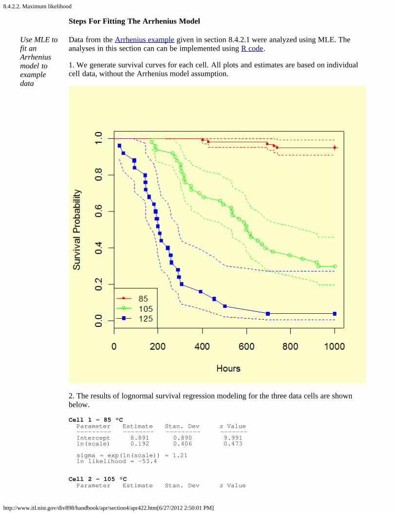
8.4.2.2. Maximum likelihood
http://www.itl.nist.gov/div898/handbook/apr/section4/apr422.htm[6/27/2012 2:50:01 PM]
Steps For Fitting The Arrhenius Model
Use MLE tofit anArrheniusmodel toexampledata
Data from the Arrhenius example given in section 8.4.2.1 were analyzed using MLE. Theanalyses in this section can can be implemented using R code.
1. We generate survival curves for each cell. All plots and estimates are based on individualcell data, without the Arrhenius model assumption.
2. The results of lognormal survival regression modeling for the three data cells are shownbelow.
Cell 1 - 85 °C Parameter Estimate Stan. Dev z Value --------- -------- --------- ------- Intercept 8.891 0.890 9.991 ln(scale) 0.192 0.406 0.473 sigma = exp(ln(scale)) = 1.21 ln likelihood = -53.4
Cell 2 - 105 °C Parameter Estimate Stan. Dev z Value
8.4.2.2. Maximum likelihood
http://www.itl.nist.gov/div898/handbook/apr/section4/apr422.htm[6/27/2012 2:50:01 PM]
--------- -------- --------- ------- Intercept 6.470 0.108 60.14 ln(scale) -0.336 0.129 -2.60 sigma = exp(ln(scale)) = 0.715 ln likelihood = -265.2
Cell 3 - 125 °C Parameter Estimate Stan. Dev z Value --------- -------- --------- ------- Intercept 5.33 0.163 32.82 ln(scale) -0.21 0.146 -1.44 sigma = exp(ln(scale)) = 0.81 ln likelihood = -156.5
The cell ln likelihood values are -53.4, -265.2 and -156.5, respectively. Adding them togetheryields a total ln likelihood of -475.1 for all the data fit with separate lognormal parameters foreach cell (no Arrhenius model assumption).
3. Fit the Arrhenius model to all data using MLE.
Parameter Estimate Stan. Dev z Value --------- -------- --------- ------- Intercept -19.906 2.3204 -8.58 l/kT 0.863 0.0761 11.34 ln(scale) -0.259 0.0928 -2.79 sigma = exp(ln(scale))Scale = 0.772 ln likelihood = -476.7
4. The likelihood ratio test statistic for the Arrhenius model fit (which also incorporates thesingle sigma acceleration assumption) is -2ln λ, where λ denotes the ratio of the likelihoodvalues with (L0), and without (L1) the Arrhenius model assumption so that
-2ln λ = -2ln (L0/L1) = -2(ln L0 - ln L1).
Using the results from steps 2 and 3, we have -2ln λ = -2(-476.7 - (-475.1)) = 3.2. Thedegrees of freedom for the Chi-Square test statistic is 6 - 3 = 3, since six parameters werereduced to three under the acceleration model assumption. The chance of obtaining a value 3.2or higher is 36.3% for a Chi-Square distribution with 3 degrees of freedom, which indicatesan acceptable model (no significant lack of fit).
This completes the Arrhenius model analysis of the three cells of data. If different cells of datahave different voltages, then a new variable "ln V" could be added as an effect to fit theInverse Power Law voltage model. In fact, several effects can be included at once if morethan one stress varies across cells. Cross product stress terms could also be included by addingthese columns to the spreadsheet and adding them in the model as additional "effects".
Example Comparing Graphical Estimates and MLE
Arrheniusexamplecomparinggraphicaland MLEmethodresults
The results from the three-stress-cell Arrhenius example using graphical and MLE methodsfor estimating parameters are shown in the table below.
Graphical Estimates MLEln T50 Sigma ln T50 Sigma
Cell 1 8.17 0.91 8.89 1.21Cell 2 6.42 0.66 6.47 0.71

8.4.2.2. Maximum likelihood
http://www.itl.nist.gov/div898/handbook/apr/section4/apr422.htm[6/27/2012 2:50:01 PM]
Cell 3 5.32 0.81 5.33 0.81
Acceleration Model Overall EstimatesH Sigma ln A
Graphical 0.808 0.74 -18.312MLE 0.863 0.77 -19.91
Note that when there are a lot of failures and little censoring, the two methods are in fairlyclose agreement. Both methods are also in close agreement on the Arrhenius model results.However, even small differences can be important when projecting reliability numbers at useconditions. In this example, the CDF at 25 °C and 100,000 hours projects to 0.014 using thegraphical estimates and only 0.003 using the MLE.
MLEmethodtests modelsand givesconfidenceintervals
The maximum likelihood method allows us to test whether parallel lines (a single sigma) arereasonable and whether the Arrhenius model is acceptable. The likelihood ratio tests for thethree example data cells indicated that a single sigma and the Arrhenius model areappropriate. In addition, we can compute confidence intervals for all estimated parametersbased on the MLE results.
8.4.2.3. Fitting models using degradation data instead of failures
http://www.itl.nist.gov/div898/handbook/apr/section4/apr423.htm[6/27/2012 2:50:03 PM]
8. Assessing Product Reliability 8.4. Reliability Data Analysis 8.4.2. How do you fit an acceleration model?
8.4.2.3. Fitting models using degradation data instead offailures
If you can fitmodels usingdegradationdata, youdon't needactual testfailures
When failure can be related directly to a change over time in a measurableproduct parameter, it opens up the possibility of measuring degradation overtime and using that data to extrapolate when failure will occur. That allows us tofit acceleration models and life distribution models without actually waiting forfailures to occur.
This overview of degradation modeling assumes you have chosen a lifedistribution model and an acceleration model and offers an alternative to theaccelerated testing methodology based on failure data, previously described. Thefollowing topics are covered.
Common assumptionsAdvantagesDrawbacksA simple methodA more accurate approach for a special caseExample
More details can be found in Nelson (1990, pages 521-544) or Tobias andTrindade (1995, pages 197-203).
Common Assumptions When Modeling Degradation Data
You need ameasurableparameterthat drifts(degrades)linearly to acriticalfailure value
Two common assumptions typically made when degradation data are modeledare the following:
1. A parameter D, that can be measured over time, drifts monotonically(upwards, or downwards) towards a specified critical value DF. When itreaches DF, failure occurs.
2. The drift, measured in terms of D, is linear over time with a slope (or rateof degradation) R, that depends on the relevant stress the unit is operatingunder and also the (random) characteristics of the unit being measured.Note: It may be necessary to define D as a transformation of somestandard parameter in order to obtain linearity - logarithms or powers aresometimes needed.
The figure below illustrates these assumptions by showing degradation plots offive units on test. Degradation readings for each unit are taken at the same fourtime points and straight lines fit through these readings on a unit-by-unit basis.These lines are then extended up to a critical (failure) degradation value. Theprojected times of failure for these units are then read off the plot. The are: t , t ,
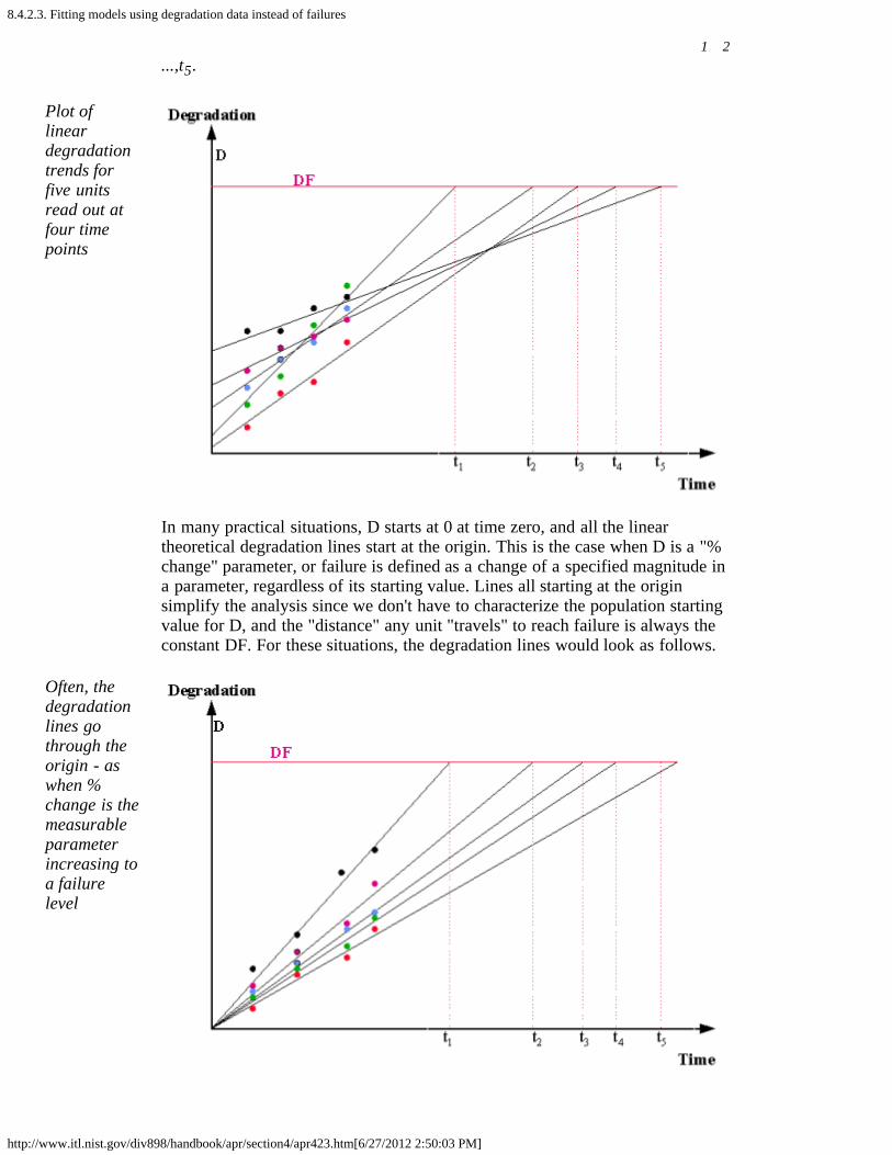
8.4.2.3. Fitting models using degradation data instead of failures
http://www.itl.nist.gov/div898/handbook/apr/section4/apr423.htm[6/27/2012 2:50:03 PM]
1 2...,t5.
Plot oflineardegradationtrends forfive unitsread out atfour timepoints
In many practical situations, D starts at 0 at time zero, and all the lineartheoretical degradation lines start at the origin. This is the case when D is a "%change" parameter, or failure is defined as a change of a specified magnitude ina parameter, regardless of its starting value. Lines all starting at the originsimplify the analysis since we don't have to characterize the population startingvalue for D, and the "distance" any unit "travels" to reach failure is always theconstant DF. For these situations, the degradation lines would look as follows.
Often, thedegradationlines gothrough theorigin - aswhen %change is themeasurableparameterincreasing toa failurelevel

8.4.2.3. Fitting models using degradation data instead of failures
http://www.itl.nist.gov/div898/handbook/apr/section4/apr423.htm[6/27/2012 2:50:03 PM]
It is also common to assume the effect of measurement error, when readingvalues of D, has relatively little impact on the accuracy of model estimates.
Advantages of Modeling Based on Degradation Data
Modelingbased oncompletesamples ofmeasurementdata, evenwith lowstress cells,offers manyadvantages
1. Every degradation readout for every test unit contributes a data point. Thisleads to large amounts of useful data, even if there are very few failures.
2. You don't have to run tests long enough to obtain significant numbers offailures.
3. You can run low stress cells that are much closer to use conditions andobtain meaningful degradation data. The same cells would be a waste oftime to run if failures were needed for modeling. Since these cells aremore typical of use conditions, it makes sense to have them influencemodel parameters.
4. Simple plots of degradation vs time can be used to visually test the lineardegradation assumption.
Drawbacks to Modeling Based on Degradation Data
Degradationmay notproceed in asmooth,linearfashiontowardswhat thecustomercalls"failure"
1. For many failure mechanisms, it is difficult or impossible to find ameasurable parameter that degrades to a critical value in such a way thatreaching that critical value is equivalent to what the customer calls afailure.
2. Degradation trends may vary erratically from unit to unit, with noapparent way to transform them into linear trends.
3. Sometimes degradation trends are reversible and a few units appear to"heal themselves" or get better. This kind of behavior does not followtypical assumptions and is difficult to model.
4. Measurement error may be significant and overwhelm small degradationtrends, especially at low stresses.
5. Even when degradation trends behave according to assumptions and thechosen models fit well, the final results may not be consistent with ananalysis based on actual failure data. This probably means that the failuremechanism depends on more than a simple continuous degradationprocess.
Because of the last listed drawback, it is a good idea to have at least one high-stress cell where enough real failures occur to do a standard life distributionmodel analysis. The parameter estimates obtained can be compared to thepredictions from the degradation data analysis, as a "reality" check.
A Simple Method For Modeling Degradation Data
A simpleapproach isto extendeach unit'sdegradationline until aprojected"failuretime" isobtained
1. As shown in the figures above, fit a line through each unit's degradationreadings. This can be done by hand, but using a least squares regressionprogram is better.
2. Take the equation of the fitted line, substitute DF for Y and solve for X.This value of X is the "projected time of fail" for that unit.
3. Repeat for every unit in a stress cell until a complete sample of(projected) times of failure is obtained for the cell.
4. Use the failure times to compute life distribution parameter estimates for acell. Under the fairly typical assumption of a lognormal model, this is verysimple. Take natural logarithms of all failure times and treat the resultingdata as a sample from a normal distribution. Compute the sample mean
8.4.2.3. Fitting models using degradation data instead of failures
http://www.itl.nist.gov/div898/handbook/apr/section4/apr423.htm[6/27/2012 2:50:03 PM]
and the sample standard deviation. These are estimates of ln T50 and σ,respectively, for the cell.
5. Assuming there are k cells with varying stress, fit an appropriateacceleration model using the cell ln T50 values, as described in thegraphical estimation section. A single sigma estimate is obtained by takingthe square root of the average of the cell σ2 estimates (assuming the samenumber of units each cell). If the cells have nj units on test, where the njvalues are not all equal, use the pooled sum-of-squares estimate across allk cells calculated by
A More Accurate Regression Approach For the Case When D = 0 at time 0and the "Distance To Fail" DF is the Same for All Units
Models canbe fit usingall thedegradationreadings andlinearregression
Let the degradation measurement for the i-th unit at the j-th readout time in thek-th stress cell be given by Dijk, and let the corresponding readout time bedenoted by tjk. That readout gives a degradation rate (or slope) estimate of D ijk/t jk. This follows from the linear assumption or:
(Rate of degradation) × (Time on test) = (Amount of degradation)
Based on that readout alone, an estimate of the natural logarithm of the time tofail for that unit is
yijk = ln DF - (ln Dijk - ln tjk).
This follows from the basic formula connecting linear degradation with failuretime
(rate of degradation) × (time of failure) = DF
by solving for (time of failure) and taking natural logarithms.
For an Arrhenius model analysis, with
with the xk values equal to 1/KT. Here T is the temperature of the k-th cell,measured in Kelvin (273.16 + degrees Celsius) and K is Boltzmann's constant(8.617 × 10⁻⁵ in eV/ unit Kelvin). Use a linear regression program to estimate a= ln A and b = ΔH. If we further assume tf has a lognormal distribution, themean square residual error from the regression fit is an estimate of σ2 (with σ thelognormal sigma).
One way to think about this model is as follows: each unit has a random rate R
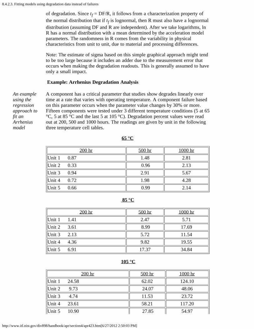
8.4.2.3. Fitting models using degradation data instead of failures
http://www.itl.nist.gov/div898/handbook/apr/section4/apr423.htm[6/27/2012 2:50:03 PM]
of degradation. Since tf = DF/R, it follows from a characterization property ofthe normal distribution that if tf is lognormal, then R must also have a lognormaldistribution (assuming DF and R are independent). After we take logarithms, lnR has a normal distribution with a mean determined by the acceleration modelparameters. The randomness in R comes from the variability in physicalcharacteristics from unit to unit, due to material and processing differences.
Note: The estimate of sigma based on this simple graphical approach might tendto be too large because it includes an adder due to the measurement error thatoccurs when making the degradation readouts. This is generally assumed to haveonly a small impact.
Example: Arrhenius Degradation Analysis
An exampleusing theregressionapproach tofit anArrheniusmodel
A component has a critical parameter that studies show degrades linearly overtime at a rate that varies with operating temperature. A component failure basedon this parameter occurs when the parameter value changes by 30% or more.Fifteen components were tested under 3 different temperature conditions (5 at 65°C, 5 at 85 °C and the last 5 at 105 °C). Degradation percent values were readout at 200, 500 and 1000 hours. The readings are given by unit in the followingthree temperature cell tables.
65 °C
200 hr 500 hr 1000 hrUnit 1 0.87 1.48 2.81Unit 2 0.33 0.96 2.13Unit 3 0.94 2.91 5.67Unit 4 0.72 1.98 4.28Unit 5 0.66 0.99 2.14
85 °C
200 hr 500 hr 1000 hrUnit 1 1.41 2.47 5.71Unit 2 3.61 8.99 17.69Unit 3 2.13 5.72 11.54Unit 4 4.36 9.82 19.55Unit 5 6.91 17.37 34.84
105 °C
200 hr 500 hr 1000 hrUnit 1 24.58 62.02 124.10Unit 2 9.73 24.07 48.06Unit 3 4.74 11.53 23.72Unit 4 23.61 58.21 117.20Unit 5 10.90 27.85 54.97
8.4.2.3. Fitting models using degradation data instead of failures
http://www.itl.nist.gov/div898/handbook/apr/section4/apr423.htm[6/27/2012 2:50:03 PM]
Note that one unit failed in the 85 °C cell and four units failed in the 105 °Ccell. Because there were so few failures, it would be impossible to fit a lifedistribution model in any cell but the 105 °C cell, and therefore no accelerationmodel can be fit using failure data. We will fit an Arrhenius/lognormal model,using the degradation data.
Solution:
Fit themodel to thedegradationdata
From the above tables, first create a variable (DEG) with 45 degradation valuesstarting with the first row in the first table and proceeding to the last row in thelast table. Next, create a temperature variable (TEMP) that has 15 repetitions of65, followed by 15 repetitions of 85 and then 15 repetitions of 105. Finally,create a time variable (TIME) that corresponds to readout times.
Fit the Arrhenius/lognormal equation, yijk = a + b xijk, where
yijk = ln(30) - (ln(DEG) - ln(TIME))and
xijk = 100000 / [8.617*(TEMP + 273.16)].
The linear regression results are the following.
Parameter Estimate Stan. Dev t Value --------- -------- --------- ------- a -18.94337 1.83343 -10.33 b 0.81877 0.05641 14.52 Residual standard deviation = 0.5611 Residual degrees of freedom = 45
The Arrhenius model parameter estimates are: ln A = -18.94; ΔH = 0.82. Anestimate of the lognormal sigma is σ = 0.56.
The analyses in this section can can be implemented using both Dataplot codeand R code.

8.4.3. How do you project reliability at use conditions?
http://www.itl.nist.gov/div898/handbook/apr/section4/apr43.htm[6/27/2012 2:50:05 PM]
8. Assessing Product Reliability 8.4. Reliability Data Analysis
8.4.3. How do you project reliability at useconditions?
Whenprojectingfrom highstress to useconditions,having acorrectaccelerationmodel andlifedistributionmodel iscritical
General Considerations
Reliability projections based on failure data from high stresstests are based on assuming we know the correct accelerationmodel for the failure mechanism under investigation and weare also using the correct life distribution model. This isbecause we are extrapolating "backwards" - trying todescribe failure behavior in the early tail of the lifedistribution, where we have little or no actual data.
For example, with an acceleration factor of 5000 (and someare much larger than this), the first 100,000 hours of use lifeis "over" by 20 hours into the test. Most, or all, of the testfailures typically come later in time and are used to fit a lifedistribution model with only the first 20 hours or less beingof practical use. Many distributions may be flexible enoughto adequately fit the data at the percentiles where the pointsare, and yet differ from the data by orders of magnitude inthe very early percentiles (sometimes referred to as the early"tail" of the distribution).
However, it is frequently necessary to test at high stress (toobtain any failures at all!) and project backwards to use.When doing this bear in mind two important points:
Project foreach failuremechanismseparately
Distribution models, and especially accelerationmodels, should be applied only to a single failuremechanism at a time. Separate out failure mechanismswhen doing the data analysis and use the competingrisk model to build up to a total component failure rateTry to find theoretical justification for the chosenmodels, or at least a successful history of their use forthe same or very similar mechanisms. (Choosingmodels solely based on empirical fit is likeextrapolating from quicksand to a mirage.)
How to Project from High Stress to Use Stress
Two types of use-condition reliability projections arecommon:
1. Projection to use conditions after completing a multiple

8.4.3. How do you project reliability at use conditions?
http://www.itl.nist.gov/div898/handbook/apr/section4/apr43.htm[6/27/2012 2:50:05 PM]
stress cell experiment and successfully fitting both alife distribution model and an acceleration model
2. Projection to use conditions after a single cell at highstress is run as a line reliability monitor.
Arrheniusmodelprojectionexample
The Arrhenius example from the graphical estimation and theMLE estimation sections ended by comparing use projectionsof the CDF at 100,000 hours. This is a projection of the firsttype. We know from the Arrhenius model assumption that theT50 at 25 °C is just
Using the graphical model estimates for ln A and we have
T50 at use = e-18.312 × e0.808 × 11605/298.16 = e13.137 = 507383
and combining this T50 with the estimate of the commonsigma of 0.74 allows us to easily estimate the CDF or failurerate after any number of hours of operation at use conditions.
In particular, the CDF value of a lognormal at T/T50 (wheretime T = 100,000, T50 = 507383, and sigma = 0.74) is 0.014,which matches the answer given in the MLE estimationsection as the graphical projection of the CDF at 100,000hours at a use temperature of 25 °C.
If the life distribution model had been Weibull, the same typeof analysis would be performed by letting the characteristiclife parameter α vary with stress according to the accelerationmodel, while the shape parameter γ is constant for all stressconditions.
The second type of use projection was used in the section onlognormal and Weibull tests, in which we judged new lots ofproduct by looking at the proportion of failures in a sampletested at high stress. The assumptions we made were:
we knew the acceleration factor between use and highstressthe shape parameter (sigma for the lognormal, gammafor the Weibull) is also known and does not changesignificantly from lot to lot.
With these assumptions, we can take any proportion offailures we see from a high stress test and project a use CDFor failure rate. For a T-hour high stress test and anacceleration factor of A from high stress to use stress, anobserved proportion p is converted to a use CDF at 100,000hours for a lognormal model using:

8.4.3. How do you project reliability at use conditions?
http://www.itl.nist.gov/div898/handbook/apr/section4/apr43.htm[6/27/2012 2:50:05 PM]
T50Stress = T×G -1(p, 0, σ) CDF = G((100000/(A×T50Stress)), 0, σ).
where G(q, μ, σ) is the lognormal distribution function withmean μ and standard deviation σ.
If the model is Weibull, we can find the use CDF or failurerate with:
AStress = T×W -1(p, γ, 1) CDF = W((100000/(A×AStress)), γ, 1).
where W(q, γ, α) is the Weibull distribution function withshape parameter γ and scale parameter α.
The analyses in this section can can be implemented usingboth Dataplot code and R code.

8.4.4. How do you compare reliability between two or more populations?
http://www.itl.nist.gov/div898/handbook/apr/section4/apr44.htm[6/27/2012 2:50:05 PM]
8. Assessing Product Reliability 8.4. Reliability Data Analysis
8.4.4. How do you compare reliability betweentwo or more populations?
Severalmethodsforcomparingreliabilitybetweenpopulationsaredescribed
Comparing reliability among populations based on samples offailure data usually means asking whether the samples camefrom populations with the same reliability function (or CDF).Three techniques already described can be used to answerthis question for censored reliability data. These are:
Comparing sample proportion failures Likelihood ratio test comparisonsLifetime regression comparisons
Comparing Sample Proportion Failures
Assume each sample is a random sample from possibly adifferent lot, vendor or production plant. All the samples aretested under the same conditions. Each has an observedproportion of failures on test. Call these sample proportions offailures p1, p2, p3, ...pn. Could these all have come fromequivalent populations?
This is a question covered in Chapter 7 for two populations,and for more than two populations, and the techniquesdescribed there apply equally well here.
Likelihood Ratio Test Comparisons
The Likelihood Ratio test was described earlier. In thisapplication, the Likelihood ratio has as a denominator theproduct of all the Likelihoods of all the samples assumingeach population has its own unique set of parameters. Thenumerator is the product of the Likelihoods assuming theparameters are exactly the same for each population. The testlooks at whether -2ln is unusually large, in which case it isunlikely the populations have the same parameters (orreliability functions).
This procedure is very effective if, and only if, it is built intothe analysis software package being used and this softwarecovers the models and situations of interest to the analyst.
Lifetime Regression Comparisons
Lifetime regression is similar to maximum likelihood and

8.4.4. How do you compare reliability between two or more populations?
http://www.itl.nist.gov/div898/handbook/apr/section4/apr44.htm[6/27/2012 2:50:05 PM]
likelihood ratio test methods. Each sample is assumed to havecome from a population with the same shape parameter and awide range of questions about the scale parameter (which isoften assumed to be a "measure" of lot-to-lot or vendor-to-vendor quality) can be formulated and tested for significance.
For a complicated, but realistic example, assume a companymanufactures memory chips and can use chips with someknown defects ("partial goods") in many applications.However, there is a question of whether the reliability of"partial good" chips is equivalent to "all good" chips. Thereexists lots of customer reliability data to answer this question.However the data are difficult to analyze because they containseveral different vintages with known reliability differencesas well as chips manufactured at many different locations.How can the partial good vs all good question be resolved?
A lifetime regression model can be constructed with variablesincluded that change the scale parameter based on vintage,location, partial versus all good, and any other relevantvariables. Then, a good lifetime regression program will sortout which, if any, of these factors are significant and, inparticular, whether there is a significant difference between"partial good" and "all good".

8.4.5. How do you fit system repair rate models?
http://www.itl.nist.gov/div898/handbook/apr/section4/apr45.htm[6/27/2012 2:50:06 PM]
8. Assessing Product Reliability 8.4. Reliability Data Analysis
8.4.5. How do you fit system repair ratemodels?
Fittingmodelsdiscussedearlier
This subsection describes how to fit system repair rate modelswhen you have actual failure data. The data could come from from observing a system in normal operation or from runningtests such as Reliability Improvement tests.
The three models covered are the constant repair rate(HPP/exponential) model, the power law (Duane) model andthe exponential law model.
8.4.5.1. Constant repair rate (HPP/exponential) model
http://www.itl.nist.gov/div898/handbook/apr/section4/apr451.htm[6/27/2012 2:50:07 PM]
8. Assessing Product Reliability 8.4. Reliability Data Analysis 8.4.5. How do you fit system repair rate models?
8.4.5.1. Constant repair rate (HPP/exponential) model
ThissectioncoversestimatingMTBF'sandcalculatingupper andlowerconfidencebounds
The HPP or exponential model is widely used for two reasons:
Most systems spend most of their useful lifetimes operating in the flatconstant repair rate portion of the bathtub curveIt is easy to plan tests, estimate the MTBF and calculate confidenceintervals when assuming the exponential model.
This section covers the following:
1. Estimating the MTBF (or repair rate/failure rate)2. How to use the MTBF confidence interval factors3. Tables of MTBF confidence interval factors 4. Confidence interval equation and "zero fails" case5. Calculation of confidence intervals6. Example
Estimating the MTBF (or repair rate/failure rate)
For the HPP system model, as well as for the non repairable exponentialpopulation model, there is only one unknown parameter (or equivalently,the MTBF = 1/ ). The method used for estimation is the same for the HPPmodel and for the exponential population model.
The bestestimate ofthe MTBFis just"TotalTime"divided by"TotalFailures"
The estimate of the MTBF is
This estimate is the maximum likelihood estimate whether the data arecensored or complete, or from a repairable system or a non-repairablepopulation.
ConfidenceIntervalFactorsmultiplytheestimated
How To Use the MTBF Confidence Interval Factors
1. Estimate the MTBF by the standard estimate (total unit test hoursdivided by total failures)
2. Pick a confidence level (i.e., pick 100x(1- )). For 95%, = .05; for90%, = .1; for 80%, = .2 and for 60%, = .4
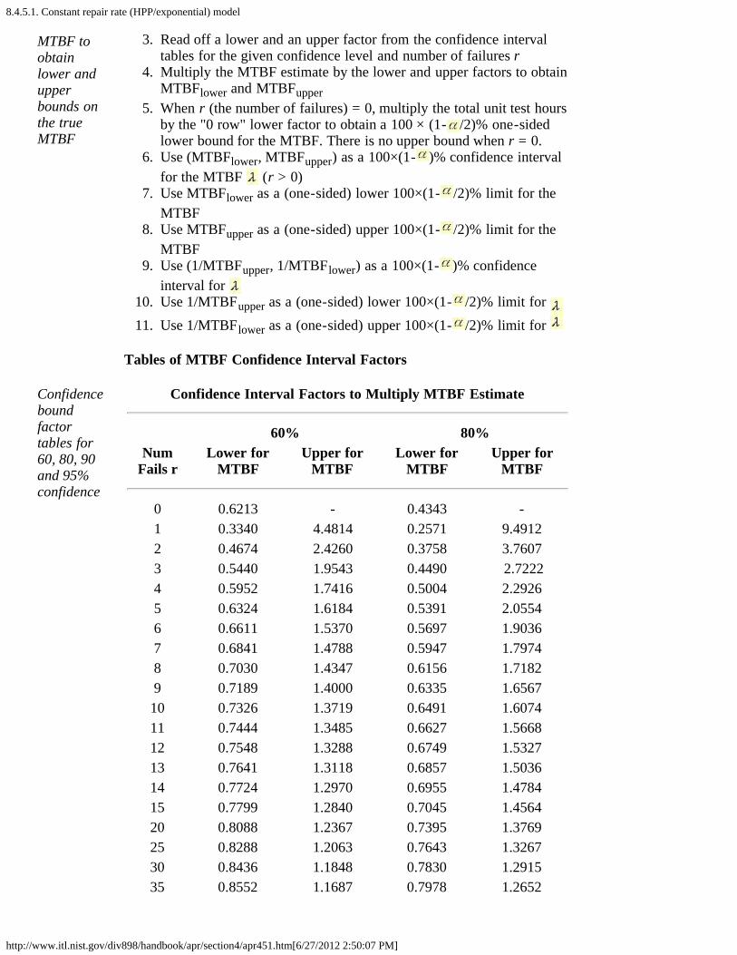
8.4.5.1. Constant repair rate (HPP/exponential) model
http://www.itl.nist.gov/div898/handbook/apr/section4/apr451.htm[6/27/2012 2:50:07 PM]
MTBF toobtainlower andupperbounds onthe trueMTBF
3. Read off a lower and an upper factor from the confidence intervaltables for the given confidence level and number of failures r
4. Multiply the MTBF estimate by the lower and upper factors to obtainMTBFlower and MTBFupper
5. When r (the number of failures) = 0, multiply the total unit test hoursby the "0 row" lower factor to obtain a 100 × (1- /2)% one-sidedlower bound for the MTBF. There is no upper bound when r = 0.
6. Use (MTBFlower, MTBFupper) as a 100×(1- )% confidence intervalfor the MTBF (r > 0)
7. Use MTBFlower as a (one-sided) lower 100×(1- /2)% limit for theMTBF
8. Use MTBFupper as a (one-sided) upper 100×(1- /2)% limit for theMTBF
9. Use (1/MTBFupper, 1/MTBFlower) as a 100×(1- )% confidenceinterval for
10. Use 1/MTBFupper as a (one-sided) lower 100×(1- /2)% limit for 11. Use 1/MTBFlower as a (one-sided) upper 100×(1- /2)% limit for
Tables of MTBF Confidence Interval Factors
Confidenceboundfactortables for60, 80, 90and 95%confidence
Confidence Interval Factors to Multiply MTBF Estimate
60% 80%Num
Fails rLower for
MTBFUpper for
MTBFLower for
MTBFUpper for
MTBF
0 0.6213 - 0.4343 -1 0.3340 4.4814 0.2571 9.4912 2 0.4674 2.4260 0.3758 3.76073 0.5440 1.9543 0.4490 2.7222 4 0.5952 1.7416 0.5004 2.29265 0.6324 1.6184 0.5391 2.05546 0.6611 1.5370 0.5697 1.90367 0.6841 1.4788 0.5947 1.79748 0.7030 1.4347 0.6156 1.7182 9 0.7189 1.4000 0.6335 1.6567
10 0.7326 1.3719 0.6491 1.607411 0.7444 1.3485 0.6627 1.566812 0.7548 1.3288 0.6749 1.5327 13 0.7641 1.3118 0.6857 1.503614 0.7724 1.2970 0.6955 1.478415 0.7799 1.2840 0.7045 1.456420 0.8088 1.2367 0.7395 1.3769 25 0.8288 1.2063 0.7643 1.3267 30 0.8436 1.1848 0.7830 1.291535 0.8552 1.1687 0.7978 1.2652
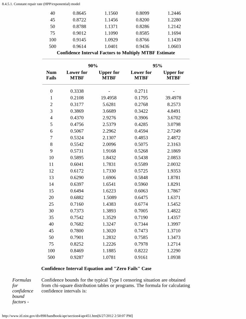
8.4.5.1. Constant repair rate (HPP/exponential) model
http://www.itl.nist.gov/div898/handbook/apr/section4/apr451.htm[6/27/2012 2:50:07 PM]
40 0.8645 1.1560 0.8099 1.244645 0.8722 1.1456 0.8200 1.2280 50 0.8788 1.1371 0.8286 1.214275 0.9012 1.1090 0.8585 1.1694
100 0.9145 1.0929 0.8766 1.1439500 0.9614 1.0401 0.9436 1.0603
Confidence Interval Factors to Multiply MTBF Estimate
90% 95%NumFails
Lower forMTBF
Upper forMTBF
Lower forMTBF
Upper forMTBF
0 0.3338 - 0.2711 -1 0.2108 19.4958 0.1795 39.4978 2 0.3177 5.6281 0.2768 8.25733 0.3869 3.6689 0.3422 4.84914 0.4370 2.9276 0.3906 3.67025 0.4756 2.5379 0.4285 3.07986 0.5067 2.2962 0.4594 2.72497 0.5324 2.1307 0.4853 2.48728 0.5542 2.0096 0.5075 2.31639 0.5731 1.9168 0.5268 2.1869
10 0.5895 1.8432 0.5438 2.085311 0.6041 1.7831 0.5589 2.003212 0.6172 1.7330 0.5725 1.935313 0.6290 1.6906 0.5848 1.878114 0.6397 1.6541 0.5960 1.829115 0.6494 1.6223 0.6063 1.786720 0.6882 1.5089 0.6475 1.637125 0.7160 1.4383 0.6774 1.545230 0.7373 1.3893 0.7005 1.482235 0.7542 1.3529 0.7190 1.435740 0.7682 1.3247 0.7344 1.399745 0.7800 1.3020 0.7473 1.371050 0.7901 1.2832 0.7585 1.347375 0.8252 1.2226 0.7978 1.2714
100 0.8469 1.1885 0.8222 1.2290500 0.9287 1.0781 0.9161 1.0938
Confidence Interval Equation and "Zero Fails" Case
Formulasforconfidenceboundfactors -
Confidence bounds for the typical Type I censoring situation are obtainedfrom chi-square distribution tables or programs. The formula for calculatingconfidence intervals is:

8.4.5.1. Constant repair rate (HPP/exponential) model
http://www.itl.nist.gov/div898/handbook/apr/section4/apr451.htm[6/27/2012 2:50:07 PM]
even for"zero fails"case
In this formula, Χ 2α/2,2r is a value that the chi-square statistic with 2r
degrees of freedom is less than with probability α/2. In other words, theleft-hand tail of the distribution has probability α/2. An even simplerversion of this formula can be written using T = the total unit test time:
These bounds are exact for the case of one or more repairable systems ontest for a fixed time. They are also exact when non repairable units are ontest for a fixed time and failures are replaced with new units during thecourse of the test. For other situations, they are approximate.
When there are zero failures during the test or operation time, only a (one-sided) MTBF lower bound exists, and this is given by
MTBFlower = T/(-ln )
The interpretation of this bound is the following: if the true MTBF wereany lower than MTBFlower, we would have seen at least one failure duringT hours of test with probability at least 1-α. Therefore, we are 100(1-α) %confident that the true MTBF is not lower than MTBFlower.
Calculationofconfidencelimits
A one-sided, lower 100(1-α/2) % confidence bound for the MTBF is givenby
LOWER = 2T/G -1(1-α/2, [2(r+1)])
where T is the total unit or system test time, r is the total number offailures, and G(q,ν) is the Χ 2 distribution function with shape parameter ν.
A one-sided, upper 100(1-α/2) % confidence bound for the MTBF is givenby
UPPER = 2T/G -1(α/2, [2r])
The two intervals together, (LOWER, UPPER), are a 100(1-α) % two-sidedconfidence interval for the true MTBF.
Please use caution when using CDF and inverse CDF functions incommercial software because some functions require left-tail probabilitiesand others require right-tail probabilities. In the left-tail case, α/2 is usedfor the upper bound because 2T is being divided by the smaller percentile,and 1-α/2 is used for the lower bound because 2T is divided by the largerpercentile. For the right-tail case, 1-α/2 is used to compute the upper bound

8.4.5.1. Constant repair rate (HPP/exponential) model
http://www.itl.nist.gov/div898/handbook/apr/section4/apr451.htm[6/27/2012 2:50:07 PM]
and α/2 is used to compute the lower bound. Our formulas for G -1(q,ν)assume the inverse CDF function requires left-tail probabilities.
Example
Exampleshowinghow tocalculateconfidencelimits
A system was observed for two calendar months of operation, during whichtime it was in operation for 800 hours and had 2 failures.
The MTBF estimate is 800/2 = 400 hours. A 90 %, two-sided confidenceinterval is given by (400×0.3177, 400×5.6281) = (127, 2251). The sameinterval could have been obtained using
LOWER = 1600/G -1(0.95,6)UPPER = 1600/G -1(0.05,4)
Note that 127 is a 95 % lower limit for the true MTBF. The customer isusually only concerned with the lower limit and one-sided lower limits areoften used for statements of contractual requirements.
Zero failsconfidencelimitcalculation
What could we have said if the system had no failures? For a 95 % lowerconfidence limit on the true MTBF, we either use the 0 failures factor fromthe 90 % confidence interval table and calculate 800 × 0.3338 = 267, or weuse T/(ln α) = 800/(ln 0.05) = 267.
The analyses in this section can can be implemented using both Dataplotcode and R code.

8.4.5.2. Power law (Duane) model
http://www.itl.nist.gov/div898/handbook/apr/section4/apr452.htm[6/27/2012 2:50:09 PM]
8. Assessing Product Reliability 8.4. Reliability Data Analysis 8.4.5. How do you fit system repair rate models?
8.4.5.2. Power law (Duane) model
The PowerLaw(Duane)model hasbeen verysuccessful inmodelingindustrialreliabilityimprovementdata
Brief Review of Power Law Model and Duane Plots
Recall that the Power Law is a NHPP with the expected number offails, M(t), and the repair rate, M'(t) = m(t), given by:
The parameter = 1-b is called the Reliability Growth Slope andtypical industry values for growth slopes during reliabilityimprovement tests are in the .3 to .6 range.
If a system is observed for a fixed time of T hours and failuresoccur at times t1, t2, t3, ..., tr (with the start of the test orobservation period being time 0), a Duane plot is a plot of (ti / i)versus ti on log-log graph paper. If the data are consistent with aPower Law model, the points in a Duane Plot will roughly follow astraight line with slope and intercept (where t = 1 on the log-logpaper) of -log10a.
MLE's forthe PowerLaw modelare given
Estimates for the Power Law Model
Computer aided graphical estimates can easily be obtained bydoing a regression fit of Y = ln (ti / i) vs X = ln ti. The slope isthe estimate and e-intercept is the a estimate. The estimate of b is
1- .
However, better estimates can easily be calculated. These aremodified maximum likelihood estimates (corrected to eliminatebias). The formulas are given below for a fixed time of T hours,and r failures occurring at times t1, t2, t3, ..., tr.
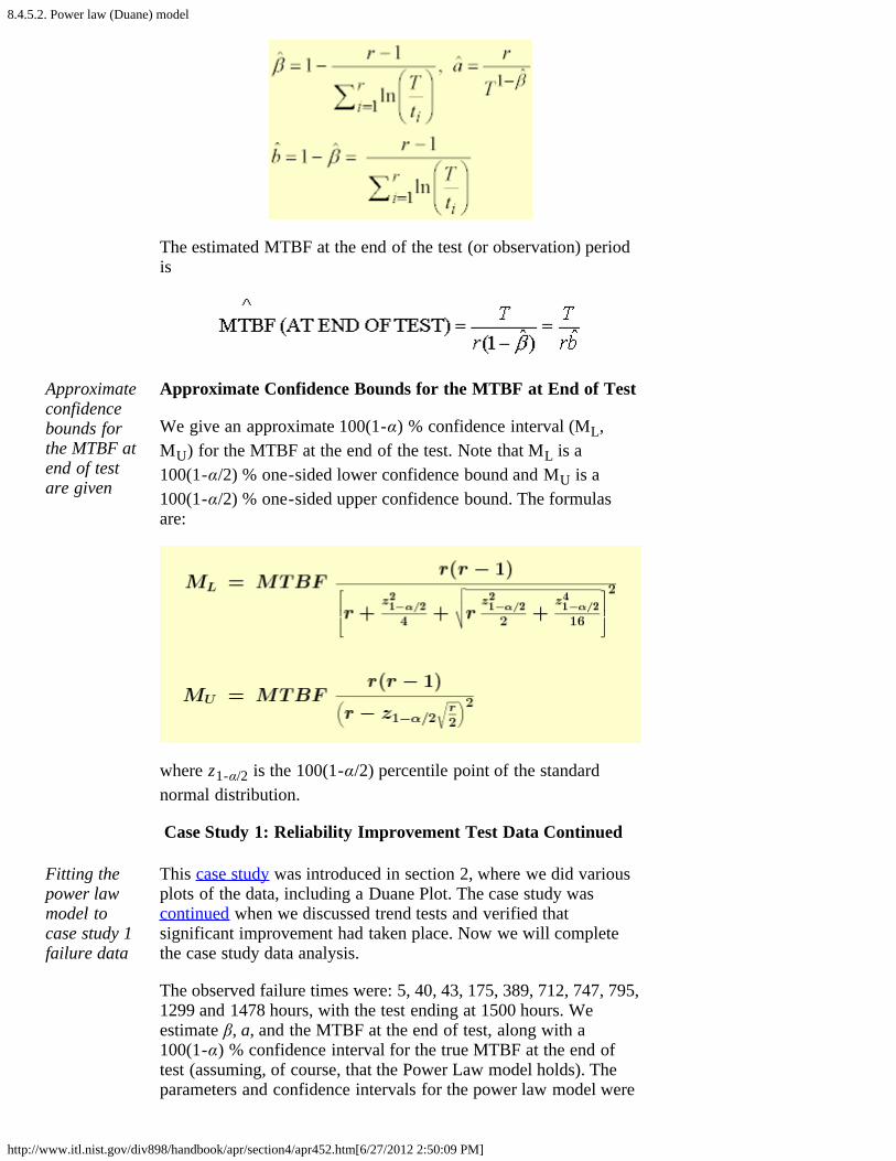
8.4.5.2. Power law (Duane) model
http://www.itl.nist.gov/div898/handbook/apr/section4/apr452.htm[6/27/2012 2:50:09 PM]
The estimated MTBF at the end of the test (or observation) periodis
Approximateconfidencebounds forthe MTBF atend of testare given
Approximate Confidence Bounds for the MTBF at End of Test
We give an approximate 100(1-α) % confidence interval (ML,MU) for the MTBF at the end of the test. Note that ML is a100(1-α/2) % one-sided lower confidence bound and MU is a100(1-α/2) % one-sided upper confidence bound. The formulasare:
where z1-α/2 is the 100(1-α/2) percentile point of the standardnormal distribution.
Case Study 1: Reliability Improvement Test Data Continued
Fitting thepower lawmodel tocase study 1failure data
This case study was introduced in section 2, where we did variousplots of the data, including a Duane Plot. The case study wascontinued when we discussed trend tests and verified thatsignificant improvement had taken place. Now we will completethe case study data analysis.
The observed failure times were: 5, 40, 43, 175, 389, 712, 747, 795,1299 and 1478 hours, with the test ending at 1500 hours. Weestimate β, a, and the MTBF at the end of test, along with a100(1-α) % confidence interval for the true MTBF at the end oftest (assuming, of course, that the Power Law model holds). Theparameters and confidence intervals for the power law model were

8.4.5.2. Power law (Duane) model
http://www.itl.nist.gov/div898/handbook/apr/section4/apr452.htm[6/27/2012 2:50:09 PM]
estimated to be the following.
Estimate of β = 0.5165 Estimate of a = 0.2913 Estimate of MTBF at the end of the test = 310.234 80 % two-sided confidence interval: (157.7139 , 548.5565)90 % one-sided lower confidence limit = 157.7139
The analyses in this section can can be implemented using R code.
8.4.5.3. Exponential law model
http://www.itl.nist.gov/div898/handbook/apr/section4/apr453.htm[6/27/2012 2:50:10 PM]
8. Assessing Product Reliability 8.4. Reliability Data Analysis 8.4.5. How do you fit system repair rate models?
8.4.5.3. Exponential law model
Estimatesof theparametersof theExponentialLaw modelcan beobtainedfrom eithera graphicalprocedureormaximumlikelihoodestimation
Recall from section 1 that the Exponential Law refers to aNHPP process with repair rate M'(t) = m(t) = . Thismodel has not been used nearly as much in industrialapplications as the Power Law model, and it is more difficultto analyze. Only a brief description will be given here.
Since the expected number of failures is given by
M(t) = and ln M(t) = , a plot of thecum fails versus time of failure on a log-linear scale shouldroughly follow a straight line with slope . Doing aregression fit of y = ln cum fails versus x = time of failurewill provide estimates of the slope and the intercept - ln
.
Alternatively, maximum likelihood estimates can be obtainedfrom the following pair of equations:
The first equation is non-linear and must be solved iterativelyto obtain the maximum likelihood estimate for . Then, thisestimate is substituted into the second equation to solve forthe maximum likelihood estimate for .
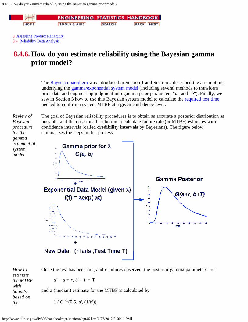
8.4.6. How do you estimate reliability using the Bayesian gamma prior model?
http://www.itl.nist.gov/div898/handbook/apr/section4/apr46.htm[6/27/2012 2:50:11 PM]
8. Assessing Product Reliability 8.4. Reliability Data Analysis
8.4.6. How do you estimate reliability using the Bayesian gammaprior model?
The Bayesian paradigm was introduced in Section 1 and Section 2 described the assumptionsunderlying the gamma/exponential system model (including several methods to transformprior data and engineering judgment into gamma prior parameters "a" and "b"). Finally, wesaw in Section 3 how to use this Bayesian system model to calculate the required test timeneeded to confirm a system MTBF at a given confidence level.
Review ofBayesianprocedurefor thegammaexponentialsystemmodel
The goal of Bayesian reliability procedures is to obtain as accurate a posterior distribution aspossible, and then use this distribution to calculate failure rate (or MTBF) estimates withconfidence intervals (called credibility intervals by Bayesians). The figure belowsummarizes the steps in this process.
How toestimatethe MTBFwithbounds,based onthe
Once the test has been run, and r failures observed, the posterior gamma parameters are:
a' = a + r, b' = b + T
and a (median) estimate for the MTBF is calculated by
1 / G -1(0.5, a', (1/b'))
8.4.6. How do you estimate reliability using the Bayesian gamma prior model?
http://www.itl.nist.gov/div898/handbook/apr/section4/apr46.htm[6/27/2012 2:50:11 PM]
posteriordistribution where G(q, γ, β) represents the gamma distribution with shape parameter γ, and scale
parameter β. Some people prefer to use the reciprocal of the mean of the posterior distributionas their estimate for the MTBF. The mean is the minimum mean square error (MSE)estimator of λ, but using the reciprocal of the mean to estimate the MTBF is always moreconservative than the "even money" 50% estimator.
A lower 80% bound for the MTBF is obtained from
1 / G -1(0.8, a', (1/b'))
and, in general, a lower 100(1-α) % lower bound is given by
1 / G -1((1-α), a', (1/b')).
A two-sided 100(1-α) % credibility interval for the MTBF is
[1 / G -1((1-α/2), a', (1/b')), 1 / G -1((α/2), a', (1/b'))].
Finally, the G((1/M), a', (1/b')) calculates the probability that MTBF is greater than M.
Example
A Bayesianexample toestimatethe MTBFandcalculateupper andlowerbounds
A system has completed a reliability test aimed at confirming a 600 hour MTBF at an 80%confidence level. Before the test, a gamma prior with a = 2, b = 1400 was agreed upon, basedon testing at the vendor's location. Bayesian test planning calculations, allowing up to 2 newfailures, called for a test of 1909 hours. When that test was run, there actually were exactlytwo failures. What can be said about the system?
The posterior gamma CDF has parameters a' = 4 and b' = 3309. The plot below shows CDFvalues on the y-axis, plotted against 1/λ = MTBF, on the x-axis. By going from probability, onthe y-axis, across to the curve and down to the MTBF, we can estimate any MTBF percentilepoint.

8.4.6. How do you estimate reliability using the Bayesian gamma prior model?
http://www.itl.nist.gov/div898/handbook/apr/section4/apr46.htm[6/27/2012 2:50:11 PM]
The MTBF values are shown below.1 / G -1(0.9, 4, (1/3309)) = 495 hours
1 / G -1(0.8, 4, (1/3309)) = 600 hours (as expected)
1 / G -1(0.5, 4, (1/3309)) = 901 hours
1 / G -1(0.1, 4, (1/3309)) = 1897 hours
The test has confirmed a 600 hour MTBF at 80 % confidence, a 495 hour MTBF at 90 %confidence and (495, 1897) is a 90 % credibility interval for the MTBF. A single number(point) estimate for the system MTBF would be 901 hours. Alternatively, you might want touse the reciprocal of the mean of the posterior distribution (b'/a') = 3309/4 = 827 hours as asingle estimate. The reciprocal mean is more conservative, in this case it is a 57 % lowerbound (G((4/3309), 4, (1/3309))).
The analyses in this section can can be implemented using R code.

8.4.6. How do you estimate reliability using the Bayesian gamma prior model?
http://www.itl.nist.gov/div898/handbook/apr/section4/apr46.htm[6/27/2012 2:50:11 PM]

8.4.7. References For Chapter 8: Assessing Product Reliability
http://www.itl.nist.gov/div898/handbook/apr/section4/apr47.htm[6/27/2012 2:50:12 PM]
8. Assessing Product Reliability 8.4. Reliability Data Analysis
8.4.7. References For Chapter 8: AssessingProduct Reliability
Aitchison, J. and Brown, J. A. C.,(1957), The Log-normal distribution, Cambridge University Press, New York and London.
Ascher, H. (1981), "Weibull Distribution vs Weibull Process,"Proceedings Annual Reliability and Maintainability Symposium, pp. 426-431.
Ascher, H. and Feingold, H. (1984), Repairable Systems Reliability,Marcel Dekker, Inc., New York.
Bain, L.J. and Englehardt, M. (1991), Statistical Analysis of Reliabilityand Life-Testing Models: Theory and Methods, 2nd ed., Marcel Dekker,New York.
Barlow, R. E. and Proschan, F. (1975), Statistical Theory of Reliabilityand Life Testing, Holt, Rinehart and Winston, New York.
Birnbaum, Z.W., and Saunders, S.C. (1968), "A ProbabilisticInterpretation of Miner's Rule," SIAM Journal of Applied Mathematics,Vol. 16, pp. 637-652.
Birnbaum, Z.W., and Saunders, S.C. (1969), "A New Family of LifeDistributions," Journal of Applied Probability, Vol. 6, pp. 319-327.
Cox, D.R. and Lewis, P.A.W. (1966), The Statistical Analysis of Seriesof Events, John Wiley & Sons, Inc., New York.
Cox, D.R. (1972), "Regression Models and Life Tables," Journal of theRoyal Statistical Society, B 34, pp. 187-220.
Cox, D. R., and Oakes, D. (1984), Analysis of Survival Data, Chapmanand Hall, London, New York.
Crow, L.H. (1974), "Reliability Analysis for Complex RepairableSystems", Reliability and Biometry, F. Proschan and R.J. Serfling, eds.,SIAM, Philadelphia, pp 379- 410.
Crow, L.H. (1975), "On Tracking Reliability Growth," ProceedingsAnnual Reliability and Maintainability Symposium, pp. 438-443.
Crow, L.H. (1982), "Confidence Interval Procedures for the WeibullProcess With Applications to Reliability Growth," Technometrics,

8.4.7. References For Chapter 8: Assessing Product Reliability
http://www.itl.nist.gov/div898/handbook/apr/section4/apr47.htm[6/27/2012 2:50:12 PM]
24(1):67-72.
Crow, L.H. (1990), "Evaluating the Reliability of Repairable Systems,"Proceedings Annual Reliability and Maintainability Symposium, pp. 275-279.
Crow, L.H. (1993), "Confidence Intervals on the Reliability ofRepairable Systems," Proceedings Annual Reliability and MaintainabilitySymposium, pp. 126-134
Duane, J.T. (1964), "Learning Curve Approach to ReliabilityMonitoring," IEEE Transactions On Aerospace, 2, pp. 563-566.
Gumbel, E. J. (1954), Statistical Theory of Extreme Values and SomePractical Applications, National Bureau of Standards AppliedMathematics Series 33, U.S. Government Printing Office, Washington,D.C.
Hahn, G.J., and Shapiro, S.S. (1967), Statistical Models in Engineering,John Wiley & Sons, Inc., New York.
Hoyland, A., and Rausand, M. (1994), System Reliability Theory, JohnWiley & Sons, Inc., New York.
Johnson, N.L., Kotz, S. and Balakrishnan, N. (1994), ContinuousUnivariate Distributions Volume 1, 2nd edition, John Wiley & Sons, Inc.,New York.
Johnson, N.L., Kotz, S. and Balakrishnan, N. (1995), ContinuousUnivariate Distributions Volume 2, 2nd edition, John Wiley & Sons, Inc.,New York.
Kaplan, E.L., and Meier, P. (1958), "Nonparametric Estimation FromIncomplete Observations," Journal of the American StatisticalAssociation, 53: 457-481.
Kalbfleisch, J.D., and Prentice, R.L. (1980), The Statistical Analysis ofFailure Data, John Wiley & Sons, Inc., New York.
Kielpinski, T.J., and Nelson, W.(1975), "Optimum Accelerated Life-Testsfor the Normal and Lognormal Life Distributins," IEEE Transactions onReliability, Vol. R-24, 5, pp. 310-320.
Klinger, D.J., Nakada, Y., and Menendez, M.A. (1990), AT&T ReliabilityManual, Van Nostrand Reinhold, Inc, New York.
Kolmogorov, A.N. (1941), "On A Logarithmic Normal Distribution LawOf The Dimensions Of Particles Under Pulverization," Dokl. Akad Nauk,USSR 31, 2, pp. 99-101.
Kovalenko, I.N., Kuznetsov, N.Y., and Pegg, P.A. (1997), MathematicalTheory of Reliability of Time Dependent Systems with PracticalApplications, John Wiley & Sons, Inc., New York.
Landzberg, A.H., and Norris, K.C. (1969), "Reliability of Controlled

8.4.7. References For Chapter 8: Assessing Product Reliability
http://www.itl.nist.gov/div898/handbook/apr/section4/apr47.htm[6/27/2012 2:50:12 PM]
Collapse Interconnections." IBM Journal Of Research and Development,Vol. 13, 3.
Lawless, J.F. (1982), Statistical Models and Methods For Lifetime Data,John Wiley & Sons, Inc., New York.
Leon, R. (1997-1999), JMP Statistical Tutorials on the Web athttp://www.nist.gov/cgi-bin/exit_nist.cgi?url=http://web.utk.edu/~leon/jmp/.
Mann, N.R., Schafer, R.E. and Singpurwalla, N.D. (1974), Methods ForStatistical Analysis Of Reliability & Life Data, John Wiley & Sons, Inc.,New York.
Martz, H.F., and Waller, R.A. (1982), Bayesian Reliability Analysis,Krieger Publishing Company, Malabar, Florida.
Meeker, W.Q., and Escobar, L.A. (1998), Statistical Methods forReliability Data, John Wiley & Sons, Inc., New York.
Meeker, W.Q., and Hahn, G.J. (1985), "How to Plan an Accelerated LifeTest - Some Practical Guidelines," ASC Basic References In QualityControl: Statistical Techniques - Vol. 10, ASQC , Milwaukee,Wisconsin.
Meeker, W.Q., and Nelson, W. (1975), "Optimum Accelerated Life-Testsfor the Weibull and Extreme Value Distributions," IEEE Transactions onReliability, Vol. R-24, 5, pp. 321-322.
Michael, J.R., and Schucany, W.R. (1986), "Analysis of Data FromCensored Samples," Goodness of Fit Techniques, ed. by D'Agostino,R.B., and Stephens, M.A., Marcel Dekker, New York.
MIL-HDBK-189 (1981), Reliability Growth Management, U.S.Government Printing Office.
MIL-HDBK-217F ((1986), Reliability Prediction of ElectronicEquipment, U.S. Government Printing Office.
MIL-STD-1635 (EC) (1978), Reliability Growth Testing, U.S.Government Printing Office.
Nelson, W. (1990), Accelerated Testing, John Wiley & Sons, Inc., NewYork.
Nelson, W. (1982), Applied Life Data Analysis, John Wiley & Sons, Inc.,New York.
O'Connor, P.D.T. (1991), Practical Reliability Engineering (ThirdEdition), John Wiley & Sons, Inc., New York.
Peck, D., and Trapp, O.D. (1980), Accelerated Testing Handbook,Technology Associates and Bell Telephone Laboratories, Portola, Calif.
Pore, M., and Tobias, P. (1998), "How Exact are 'Exact' Exponential

8.4.7. References For Chapter 8: Assessing Product Reliability
http://www.itl.nist.gov/div898/handbook/apr/section4/apr47.htm[6/27/2012 2:50:12 PM]
System MTBF Confidence Bounds?", 1998 Proceedings of the Section onPhysical and Engineering Sciences of the American StatisticalAssociation.
SEMI E10-0701, (2001), Standard For Definition and Measurement ofEquipment Reliability, Availability and Maintainability (RAM),Semiconductor Equipment and Materials International, Mountainview,CA.
Tobias, P. A., and Trindade, D. C. (1995), Applied Reliability, 2ndedition, Chapman and Hall, London, New York.