7 large-scale convex optimization for c-ransfaculty.sist.shanghaitech.edu.cn/faculty/shiym/... · 7...

9781107142664c07 CUP/QUEK-L1 September 3, 2016 13:33 Page-149

7 Large-Scale Convex Optimization forC-RANsYuanming Shi, Jun Zhang, Khaled B. Letaief, Bo Bai, and Wei Chen

7.1 Introduction

7.1.1 C-RANs

The proliferation of “smart” mobile devices, coupled with new types of wireless appli-cations, has led to an exponential growth in wireless and mobile data traffic. In orderto provide high-volume and diversified data services, C-RAN [1, 2] has been proposed;it enables efficient interference management and resource allocation by shifting all thebaseband units (BBUs) to a single cloud data center, i.e., by forming a BBU pool withpowerful shared computing resources. Therefore, with efficient hardware utilization atthe BBU pool, a substantial reduction can be obtained in both the CAPEX (e.g., vialow-cost site construction) and the OPEX (e.g., via centralized cooling). Furthermore,the powerful conventional base stations are replaced by light and low-cost remote radioheads (RRHs), with the basic functionalities of signal transmission and reception, whichare then connected to the BBU pool by high-capacity and low-latency optical fronthaullinks. The capacity of C-RANs can thus be significantly improved through networkdensification and large-scale centralized signal processing at the BBU pool. By furtherpushing a substantial amount of data, storage, and computing resources (e.g., the radioaccess units and end-user devices) to the edge of the network, using the principle ofmobile edge computing (i.e., fog computing) [3], heterogeneous C-RANs [4], as wellas Fog-RANs and MENG-RANs [5] can be formed. These evolved architectures willfurther improve user experience by offering on-demand and personalized services andlocation-aware and content-aware applications. In this chapter we investigate the com-putation aspects of this new network paradigm, and in particular focus on the large-scaleconvex optimization for signal processing and resource allocation in C-RANs.

7.1.2 Large-Scale Convex Optimization: Challenges and Previous Work

Convex optimization serves as an indispensable tool for resource allocation and sig-nal processing in wireless networks [6–9]. For instance, coordinated beamforming [10]often yields a convex optimization formulation, i.e., second-order cone programming(SOCP) [11]. The network max–min fairness-rate optimization [12] can be solvedthrough the bisection method [11], in polynomial time; in this method a sequenceof convex subproblems needs to be solved. Furthermore, convex relaxation provides


150 Large-Scale Convex Optimization for C-RANs

a principled way to develop polynomial-time algorithms for non-convex or NP-hardproblems, e.g., group-sparsity penalty relaxation for NP-hard mixed-integer non-linearprogramming problems [2], semidefinite relaxation [7] for NP-hard robust beamforming[13, 14] and multicast beamforming [15], and a sequential convex approximation to thehighly intractable stochastic coordinated beamforming problem [16].

Nevertheless, in dense C-RANs [5], which may possibly need to handle hundreds ofRRHs simultaneously, resource allocation and signal processing problems will be dra-matically scaled up. The underlying optimization problems will have a high dimensionand/or a large number of constraints, e.g., per-RRH transmit power constraints and per-MU (mobile user) QoS constraints. For instance, for a C-RAN with 100 single-antennaRRHs and 100 single-antenna MUs, the dimension of the aggregative coordinated beam-forming vector of the optimization variables will be 104. Most advanced off-the-shelfsolvers (e.g., SeDuMi [17], SDPT3 [18], and MOSEK [19]) are based on the interior-point method. However, the computational burden of such a second-order methodmakes it inapplicable for large-scale problems. For instance, solving convex quadraticprograms has cubic complexity [20]. Furthermore, to use these solvers the original prob-lems need to be transformed to the standard forms supported by the solvers. Althoughparser/solver modeling frameworks such as CVX [21] and YALMIP [22] can auto-matically transform original problem instances into standard forms, they may requiresubstantial time to perform such a transformation [23], especially for problems with alarge number of constraints [24].

One may also develop custom algorithms to enable efficient computation by exploit-ing the structures of specific problems. For instance, the uplink–downlink duality[10] can be exploited to extract the structures of optimal beamformers [25] andenable efficient algorithms. However, such an approach still has cubic complexitysince it performs matrix inversion at each iteration [26]. First-order methods, e.g.,the alternating-direction method of multipliers (ADMM) algorithm [27], have recentlyattracted attention for their distributed and parallelizable implementation as well as fortheir capability of scaling to large problem sizes. However, most existing ADMM-basedalgorithms cannot provide the certificates of infeasibility [13, 26, 28] which are neededfor such problems as max–min rate maximization [24] and group sparse beamforming[2]. Furthermore, some of these algorithms may still fail to scale to large problem sizes,owing to SOCP subproblems [28] or semidefinite programming (SDP) subproblems [13]needed to be solved at each iteration.

Without efficient and scalable algorithms, previous studies of wireless coopera-tive networks either only demonstrate performance in small-size networks, typicallywith less than 10 RRHs, or resort to suboptimal algorithms, e.g., zero-forcing-basedapproaches [29, 30]. Meanwhile, from the above discussion, we see that the large-scaleoptimization algorithms to be developed should possess the following two features:

• they should scale well to large problem sizes with parallel computing capability;• they should detect problem infeasibility effectively, i.e., provide certificates of

infeasibility.


7.1 Introduction 151

Transformationcone

ADMM Solverx*

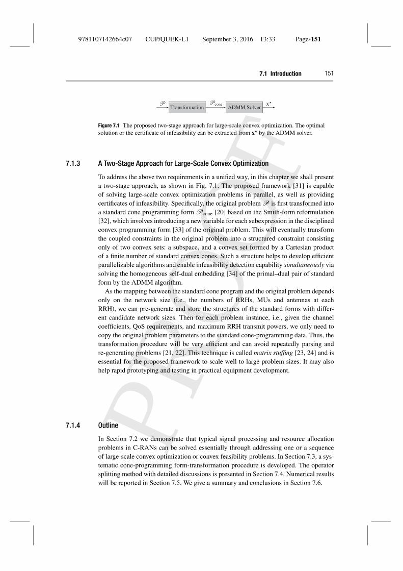
Figure 7.1 The proposed two-stage approach for large-scale convex optimization. The optimalsolution or the certificate of infeasibility can be extracted from x� by the ADMM solver.

7.1.3 A Two-Stage Approach for Large-Scale Convex Optimization

To address the above two requirements in a unified way, in this chapter we shall presenta two-stage approach, as shown in Fig. 7.1. The proposed framework [31] is capableof solving large-scale convex optimization problems in parallel, as well as providingcertificates of infeasibility. Specifically, the original problem P is first transformed intoa standard cone programming form Pcone [20] based on the Smith-form reformulation[32], which involves introducing a new variable for each subexpression in the disciplinedconvex programming form [33] of the original problem. This will eventually transformthe coupled constraints in the original problem into a structured constraint consistingonly of two convex sets: a subspace, and a convex set formed by a Cartesian productof a finite number of standard convex cones. Such a structure helps to develop efficientparallelizable algorithms and enable infeasibility detection capability simultaneously viasolving the homogeneous self-dual embedding [34] of the primal–dual pair of standardform by the ADMM algorithm.

As the mapping between the standard cone program and the original problem dependsonly on the network size (i.e., the numbers of RRHs, MUs and antennas at eachRRH), we can pre-generate and store the structures of the standard forms with differ-ent candidate network sizes. Then for each problem instance, i.e., given the channelcoefficients, QoS requirements, and maximum RRH transmit powers, we only need tocopy the original problem parameters to the standard cone-programming data. Thus, thetransformation procedure will be very efficient and can avoid repeatedly parsing andre-generating problems [21, 22]. This technique is called matrix stuffing [23, 24] and isessential for the proposed framework to scale well to large problem sizes. It may alsohelp rapid prototyping and testing in practical equipment development.

7.1.4 Outline

In Section 7.2 we demonstrate that typical signal processing and resource allocationproblems in C-RANs can be solved essentially through addressing one or a sequenceof large-scale convex optimization or convex feasibility problems. In Section 7.3, a sys-tematic cone-programming form-transformation procedure is developed. The operatorsplitting method with detailed discussions is presented in Section 7.4. Numerical resultswill be reported in Section 7.5. We give a summary and conclusions in Section 7.6.



7.2 Large-Scale Convex Optimization in Dense C-RANs

Consider the following parametric family P of convex optimization problems:

P : minimizex

f0(x; α)

s. t. fi(x; α) ≤ gi(x; α), i = 1, . . . , m, (7.1)

ui(x; α) = vi(x; α), i = 1, . . . , p, (7.2)

where x ∈ Rn is the vector of optimization variables and α ∈ A is the problem parame-

ter vector; A denotes the parameter space. For each fixed α ∈ A, the problem instanceP(α) is convex if the functions fi and gi are convex and concave, respectively, andthe functions ui and vi are affine. The reader should refer to [11] for an introductionto the basics of convex optimization. In this section we will first illustrate that typicaloptimization problems in C-RANs can be formulated in this parametric form of convexprogramming, and then the proposed framework for large-scale convex optimizationwill be introduced.

7.2.1 Convex Optimization Examples in C-RANs

To illustrate the wide-ranging applications of convex optimization in C-RANs, wemainly focus on the generic scenario for downlink transmission with full cooperationamong the RRHs. The proposed methodology in this chapter can be easily applied touplink transmission and more general cooperation scenarios in heterogeneous C-RANs[4, 8], Fog-RANs, and MENG-RANs [5] as we need only exploit the convexity of theresulting optimization problems.

Signal ModelConsider a downlink fully cooperative C-RAN with L multi-antenna RRHs and Ksingle-antenna MUs, where the lth RRH is equipped with Nl antennas. The wirelesspropagation channel from the lth RRH to the kth MU is denoted as hkl ∈ C

Nl , ∀k, l. Thereceived signal yk ∈ C at MU k is given by

yk =L∑

l=1

hHklvlksk +

∑i �=k

L∑l=1

hHklvlisi + nk, ∀k, (7.3)

where sk is the encoded information symbol for MU k with E{|sk|2} = 1, vlk ∈ CNl is

the transmit beamforming vector from the lth RRH to the kth MU, and nk ∼ CN (0, σ 2k )

is the additive Gaussian noise at MU k.We assume that the sk and nk are mutually independent and that all the users apply

single-user detection. Therefore, the signal-to-interference-plus-noise ratio (SINR) ofMU k is given by

SINRk(v1, . . . , vK) = |hHk vk|2∑

i �=k |hHk vi|2 + σ 2

k

, ∀k, (7.4)


7.2 Large-Scale Convex Optimization in Dense C-RANs 153

where hk � [hTk1 · · · hT

kL]T ∈ CN , with N = ∑L

l=1 Nl, is the channel vector consisting ofthe channel coefficients from all the RRHs to the kth MU and vk � [vT

1kvT2k · · · vT

Lk]T ∈C

N is the beamforming vector consisting of the beamforming coefficients from all theRRHs to MU k.

Coordinated beamforming is an efficient way to design energy-efficient and spectrallyefficient systems [10] in which the beamforming vectors vlk are designed to minimizethe network power consumption and maximize the network utility, respectively. Threerepresentative examples are given below to illustrate the power of convex optimizationto design efficient transmit strategies to optimize the system performance of C-RANs,for which coordinated beamforming is the basic building block.

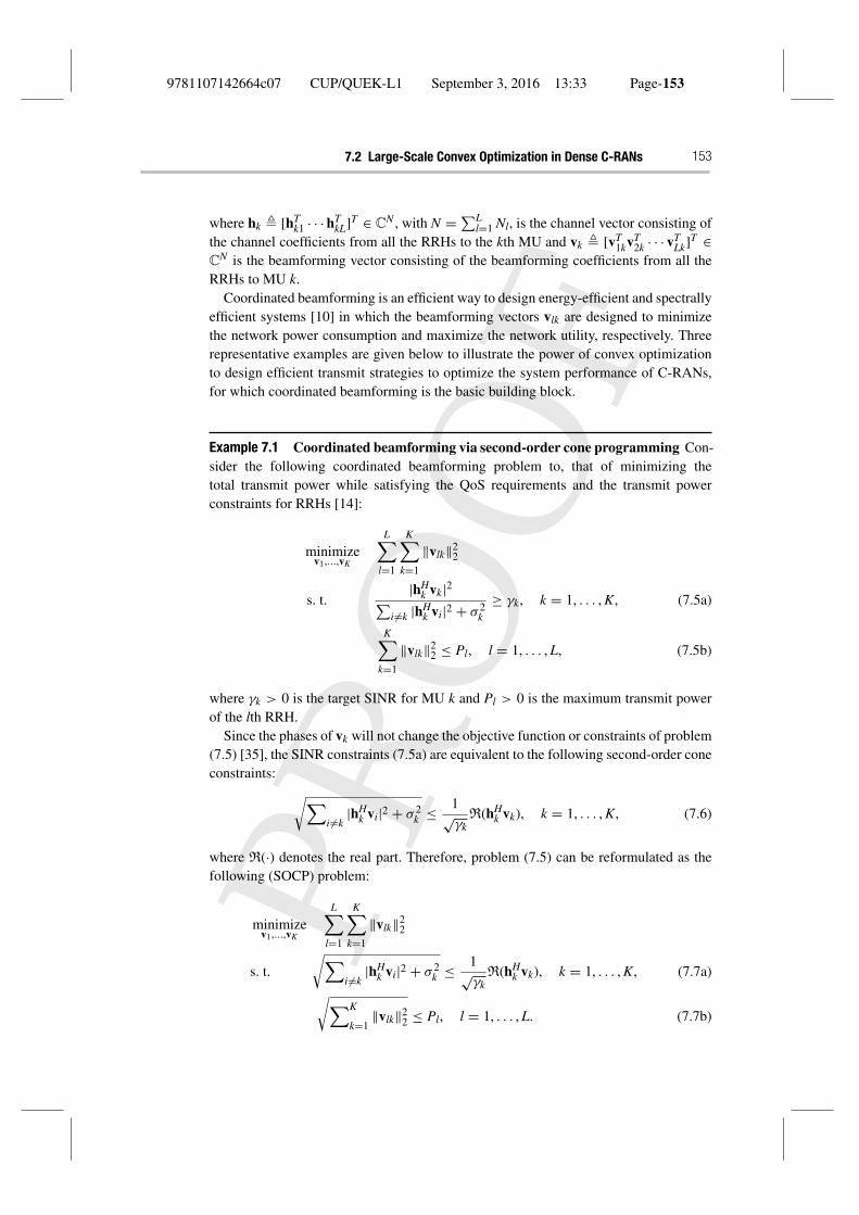
Example 7.1 Coordinated beamforming via second-order cone programming Con-sider the following coordinated beamforming problem to, that of minimizing thetotal transmit power while satisfying the QoS requirements and the transmit powerconstraints for RRHs [14]:

minimizev1,...,vK

L∑l=1

K∑k=1

‖vlk‖22

s. t.|hH

k vk|2∑i �=k |hH

k vi|2 + σ 2k

≥ γk, k = 1, . . . , K, (7.5a)

K∑k=1

‖vlk‖22 ≤ Pl, l = 1, . . . , L, (7.5b)

where γk > 0 is the target SINR for MU k and Pl > 0 is the maximum transmit powerof the lth RRH.

Since the phases of vk will not change the objective function or constraints of problem(7.5) [35], the SINR constraints (7.5a) are equivalent to the following second-order coneconstraints: √∑

i �=k|hH

k vi|2 + σ 2k ≤ 1√

γkR(hH

k vk), k = 1, . . . , K, (7.6)

where R(·) denotes the real part. Therefore, problem (7.5) can be reformulated as thefollowing (SOCP) problem:

minimizev1,...,vK

L∑l=1

K∑k=1

‖vlk‖22

s. t.

√∑i �=k

|hHk vi|2 + σ 2

k ≤ 1√γk

R(hHk vk), k = 1, . . . , K, (7.7a)√∑K

k=1‖vlk‖2

2 ≤ Pl, l = 1, . . . , L. (7.7b)



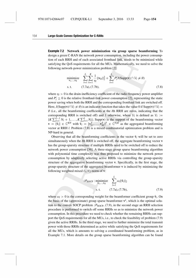
Example 7.2 Network power minimization via group sparse beamforming Todesign a green C-RAN the network power consumption, including the power consump-tion of each RRH and of each associated fronthaul link, needs to be minimized whilesatisfying the QoS requirements for all the MUs. Mathematically, we need to solve thefollowing network-power minimization problem [2]:

minimizev1,...,vK

L∑l=1

K∑k=1

1

ηl‖vlk‖2

2 +L∑

l=1

Pcl I(Supp(v) ∩ Vl �= ∅)

s. t. (7.7a), (7.7b), (7.8)

where ηl > 0 is the drain-inefficiency coefficient of the radio frequency power amplifierand Pc

l ≥ 0 is the relative fronthaul-link power consumption [2], representing the staticpower saving when both the RRH and the corresponding fronthaul link are switched off.Here, I(Supp(v)∩Vl �= ∅) is an indicator function that takes the value 0 if Supp(v)∩Vl =∅ (i.e., all the beamforming coefficients at the lth RRH are zeros, indicating that thecorresponding RRH is switched off) and 1 otherwise, where Vl is defined as Vl :={K ∑L−1

l=1 Nl + 1, . . . , K∑L

l=1 Nl}; Supp(v) is the support of the beamforming vectorv = [vl] ∈ C

KN with vl = [vTl1, . . . , vT

lK]T ∈ CNlK as the aggregated beamforming

vector at RRH l. Problem (7.8) is a mixed combinatorial optimization problem and isNP-hard in general.

Observing that all the beamforming coefficients in the vector vl will be set to zerosimultaneously when the lth RRH is switched off, the aggregate beamforming vector vhas the group-sparsity structure if multiple RRHs need to be switched off to reduce thenetwork power consumption [36]. A three-stage group sparse beamforming algorithmwith polynomial time complexity was thus proposed to minimize the network powerconsumption by adaptively selecting active RRHs via controlling the group-sparsitystructure of the aggregative beamforming vector v. Specifically, in the first stage, thegroup-sparsity structure of the aggregated beamformer v is induced by minimizing thefollowing weighted mixed �1/�2-norm of v:

PSOCP : minimizev1,...,vK

L∑l=1

ωl‖vl‖2

s. t. (7.7a), (7.7b), (7.9)

where ωl > 0 is the corresponding weight for the beamformer coefficient group vl. Onthe basis of the (approximate) group sparse beamformer v�, which is the optimal solu-tion to the convex SOCP problem PSOCP, (7.9), in the second stage an RRH selectionprocedure is performed to switch off some RRHs so as to minimize the network powerconsumption. In this procedure we need to check whether the remaining RRHs can sup-port the QoS requirements for all the MUs, i.e., to check the feasibility of problem (7.9)given the active RRHs. In the third stage, we need to further minimize the total transmitpower with those RRHs determined as active while satisfying the QoS requirements forall the MUs, which is amounts to solving a coordinated beamforming problem, as inExample 7.1. More details on the group sparse beamforming algorithm can be found


7.2 Large-Scale Convex Optimization in Dense C-RANs 155

in [2]. Extensions on semidefinite programming for network power minimization withimperfect channel state information in multicast C-RANs can be found in [14].

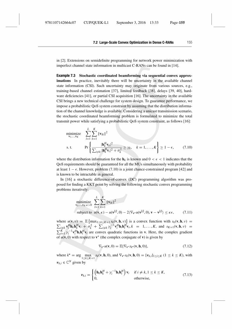
Example 7.3 Stochastic coordinated beamforming via sequential convex approx-imations In practice, inevitably there will be uncertainty in the available channelstate information (CSI). Such uncertainty may originate from various sources, e.g.,training-based channel estimation [37], limited feedback [38], delays [39, 40], hard-ware deficiencies [41], or partial CSI acquisition [16]. The uncertainty in the availableCSI brings a new technical challenge for system design. To guarantee performance, weimpose a probabilistic QoS system constraint by assuming that the distribution informa-tion of the channel knowledge is available. Considering a unicast transmission scenario,the stochastic coordinated beamforming problem is formulated to minimize the totaltransmit power while satisfying a probabilistic QoS system constraint, as follows [16]:

minimizev1,...,vK

L∑l=1

K∑k=1

‖vlk‖2

s. t. Pr

{|hH

k vk|2∑i �=k |hH

k vi|2 + σ 2k

≥ γk, k = 1, . . . , K

}≥ 1 − ε, (7.10)

where the distribution information for the hk is known and 0 < ε < 1 indicates that theQoS requirements should be guaranteed for all the MUs simultaneously with probabilityat least 1 − ε. However, problem (7.10) is a joint chance-constrained program [42] andis known to be intractable in general.

In [16] a stochastic difference-of-convex (DC) programming algorithm was pro-posed for finding a KKT point by solving the following stochastic convex programmingproblems iteratively:

minimizev1,...,vK ,κ>0

L∑l=1

K∑k=1

‖vlk‖2

subject to u(v, κ) − u(v[j], 0) − 2〈∇v∗u(v[j], 0), v − v[j]〉 ≤ κε, (7.11)

where u(v, ν) = E{max1≤k≤K+1 sk(v, h, ν)

}is a convex function with sk(v, h, ν) =∑

i �=k vHi hkhH

k vi + σ 2k + ∑

i �=k γ −1i vH

i hihHi vi, k = 1, . . . , K, and sK+1(v, h, ν) =∑K

i=1 γ −1i vH

i hihHi vi are convex quadratic functions in v. Here, the complex gradient

of u(v, 0) with respect to v∗ (the complex conjugate of v) is given by

∇v∗u(v, 0) = E{∇v∗sk�(v, h, 0)}, (7.12)

where k� = arg max1≤k≤K+1

sk(v, h, 0), and ∇v∗sk(v, h, 0) = [νk,i]1≤i≤K (1 ≤ k ≤ K), with

νk,i ∈ CN given by

νk,i ={(

hkhHk + γ −1

i hihHi

)vi if i �= k, 1 ≤ k ≤ K,

0, otherwise,(7.13)



and ∇v∗sK+1(v, h, κ) = [νK+1,i]1≤i≤K with νK+1,i = γ −1i hihH

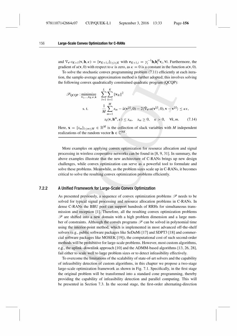
i vi, ∀i. Furthermore, thegradient of u(v, 0) with respect to κ is zero, as κ = 0 is a constant in the function u(v, 0).

To solve the stochastic convex programming problem (7.11) efficiently at each itera-tion, the sample-average approximation method is further adopted; this involves solvingthe following convex quadratically constrained quadratic program (QCQP):

PQCQP : minimizev1,...,vK ,κ ,x

L∑l=1

K∑k=1

‖vlk‖2

s. t.1

M

M∑m=1

xm − u(v[j], 0) − 2〈∇v∗u(v[j], 0), v − v[j]〉 ≤ κε,

sk(v, hm, κ) ≤ xm, xm ≥ 0, κ > 0, ∀k, m. (7.14)

Here, x = [xm]1≤m≤M ∈ RM is the collection of slack variables with M independent

realizations of the random vector h ∈ CNK .

More examples on applying convex optimization for resource allocation and signalprocessing in wireless cooperative networks can be found in [8, 9, 31]. In summary, theabove examples illustrate that the new architecture of C-RANs brings up new designchallenges, while convex optimization can serve as a powerful tool to formulate andsolve these problems. Meanwhile, as the problem sizes scale up in C-RANs, it becomescritical to solve the resulting convex optimization problems efficiently.

7.2.2 A Unified Framework for Large-Scale Convex Optimization

As presented previously, a sequence of convex optimization problems P needs to besolved for typical signal processing and resource allocation problems in C-RANs. Indense C-RANs the BBU pool can support hundreds of RRHs for simultaneous trans-mission and reception [1]. Therefore, all the resulting convex optimization problemsP are shifted into a new domain with a high problem dimension and a large num-ber of constraints. Although the convex programs P can be solved in polynomial timeusing the interior-point method, which is implemented in most advanced off-the-shelfsolvers (e.g., public software packages like SeDuMi [17] and SDPT3 [18] and commer-cial software packages like MOSEK [19]), the computational cost of such second-ordermethods will be prohibitive for large-scale problems. However, most custom algorithms,e.g., the uplink–downlink approach [10] and the ADMM-based algorithms [13, 26, 28],fail either to scale well to large problem sizes or to detect infeasibility effectively.

To overcome the limitations of the scalability of state-of-art solvers and the capabilityof infeasibility detection of custom algorithms, in this chapter we propose a two-stagelarge-scale optimization framework as shown in Fig. 7.1. Specifically, in the first stagethe original problem will be transformed into a standard cone programming, therebyproviding the capability of infeasibility detection and parallel computing. This willbe presented in Section 7.3. In the second stage, the first-order alternating-direction


7.3 Matrix Stuffing for Fast Cone-Programming Transformation 157

method of multipliers (ADMM) algorithm [27], i.e., the operator splitting method, willbe adopted to solve the large-scale homogeneous self-dual embedding (HSD) system.This will be presented in Section 7.4.

7.3 Matrix Stuffing for Fast Cone-Programming Transformation

Consider the following parametric family Pcone of primal conic optimization problems:

Pcone : minimizeν,μ

cTν

s. t. Aν + μ = b, (7.15a)

(ν, μ) ∈ Rn × K, (7.15b)

where ν ∈ Rn and μ ∈ R

m (with n ≤ m) are the optimization variables, A ∈ Rm×n,

b ∈ Rm, c ∈ R

n, and K = K1 ×· · ·×Kq ∈ Rm is a Cartesian product of q closed convex

cones. Here, each Ki has dimension mi such that∑q

i=1 mi = m. Let β = {A, b, c} ∈ Dbe the problem data with D as the data space.

Although Ki is allowed to be any closed convex cone, we are primarily interested inthe following symmetric cones:

• the nonnegative reals, R+ = {x ∈ R|x ≥ 0};• a second-order cone, Qd = {(y, x) ∈ R × R

d−1|‖x‖ ≤ y};• a positive semidefinite cone, Sn+ = {X ∈ R

n×n|X = XT , X � 0}.In particular, a problem instance Pcone(β) is known as a linear program (LP), SOCP, orSDP if all the cones Ki are restricted to R+, Qd, or Sn+, respectively. Therefore, almostall the original convex optimization problem family P can be equivalently transformedinto the standard conic optimization problem family Pcone on the basis of the princi-ple of disciplined convex programming [33]. This equivalence means that the optimalsolution or the certificate of infeasibility of the original problem instance P(α) canbe extracted from the solution to the corresponding equivalent cone-program instancePcone(β).

To develop a generic large-scale convex optimization framework, instead of exploit-ing the special structures in the original specific problems P , we propose to work withthe transformed equivalent standard conic optimization problems Pcone. This approachbears the following advantages.

1. The convex programs P can be equivalently transformed into the standard coneprograms Pcone. This will be presented in Section 7.3.1.

2. The homogeneous self-dual embedding of the primal–dual pair of the standard coneprogram Pcone can be induced, thereby providing certificates of infeasibility. Thiswill be presented in Section 7.4.1.

3. The feasible set in Pcone is formed by two sets: a subspace constraint (7.15a) and aconvex cone K, which is formed by the Cartesian product of smaller convex cones.



This salient feature will be exploited to enable parallel and scalable computing inSection 7.4.2.

7.3.1 Standard Conic Optimization Transformation

Our goal is to map the parameters α in the original convex optimization problem familyP to the problem data β in the equivalent standard conic optimization problem familyPcone with the description of the convex cone K. The general idea of such a transfor-mation is to rewrite the original problem family P in a Smith form by introducing anew variable for each subexpression in the disciplined convex programming form [33]of the problem family P . In the following we will take the coordinated beamformingproblem as an example to illustrate such a transformation.

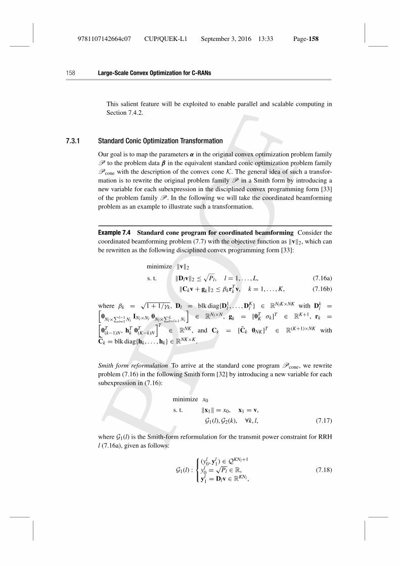
Example 7.4 Standard cone program for coordinated beamforming Consider thecoordinated beamforming problem (7.7) with the objective function as ‖v‖2, which canbe rewritten as the following disciplined convex programming form [33]:

minimize ‖v‖2

s. t. ‖Dlv‖2 ≤ √Pl, l = 1, . . . , L, (7.16a)

‖Ckv + gk‖2 ≤ βkrTk v, k = 1, . . . , K, (7.16b)

where βk = √1 + 1/γk, Dl = blk diag{D1

l , . . . , DKl } ∈ R

NlK×NK with Dkl =[

0Nl×∑l−1i=1 Ni

INl×Nl 0Nl×∑Li=l+1 Ni

]∈ R

Nl×N , gk = [0TK σk]T ∈ R

K+1, rk =[0T

(k−1)N , hTk 0T

(K−k)N

]T ∈ RNK , and Ck = [Ck 0NK]T ∈ R

(K+1)×NK with

Ck = blk diag{hk, . . . , hk} ∈ RNK×K .

Smith form reformulation To arrive at the standard cone program Pcone, we rewriteproblem (7.16) in the following Smith form [32] by introducing a new variable for eachsubexpression in (7.16):

minimize x0

s. t. ‖x1‖ = x0, x1 = v,

G1(l),G2(k), ∀k, l, (7.17)

where G1(l) is the Smith-form reformulation for the transmit power constraint for RRHl (7.16a), given as follows:

G1(l) :

⎧⎨⎩(yl

0, yl1) ∈ QKNl+1

yl0 = √

Pl ∈ R,yl

1 = Dlv ∈ RKNl ,

(7.18)



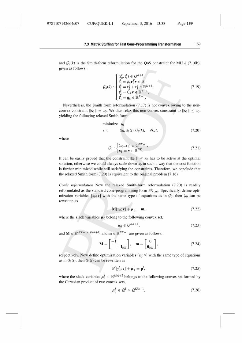
and G2(k) is the Smith-form reformulation for the QoS constraint for MU k (7.16b),given as follows:

G2(k) :

⎧⎪⎪⎪⎪⎪⎨⎪⎪⎪⎪⎪⎩

(tk0, tk1) ∈ QK+1,

tk0 = βkrTk v ∈ R,

tk1 = tk

2 + tk3 ∈ R

K+1,tk2 = Ckv ∈ R

K+1,tk3 = gk ∈ R

K+1.

(7.19)

Nevertheless, the Smith form reformulation (7.17) is not convex owing to the non-convex constraint ‖x1‖ = x0. We thus relax this non-convex constraint to ‖x1‖ ≤ x0,yielding the following relaxed Smith form:

minimize x0

s. t. G0,G1(l),G2(k), ∀k, l, (7.20)

where

G0 :

{(x0, x1) ∈ QNK+1,x1 = v ∈ R

NK .(7.21)

It can be easily proved that the constraint ‖x1‖ ≤ x0 has to be active at the optimalsolution, otherwise we could always scale down x0 in such a way that the cost functionis further minimized while still satisfying the constraints. Therefore, we conclude thatthe relaxed Smith form (7.20) is equivalent to the original problem (7.16).

Conic reformulation Now the relaxed Smith-form reformulation (7.20) is readilyreformulated as the standard cone-programming form Pcone. Specifically, define opti-mization variables [x0; v] with the same type of equations as in G0; then G0 can berewritten as

M[x0; v] + μ0 = m, (7.22)

where the slack variables μ0 belong to the following convex set,

μ0 ∈ QNK+1, (7.23)

and M ∈ R(NK+1)×(NK+1) and m ∈ R

NK+1 are given as follows:

M =[−1

−INK

], m =

[0

0NK

], (7.24)

respectively. Now define optimization variables [yl0; v] with the same type of equations

as in G1(l); then G1(l) can be rewritten as

Pl[yl0; v] + μl

1 = pl, (7.25)

where the slack variables μl1 ∈ R

KNl+2 belongs to the following convex set formed bythe Cartesian product of two convex sets,

μl1 ∈ Q1 × QKNl+1, (7.26)



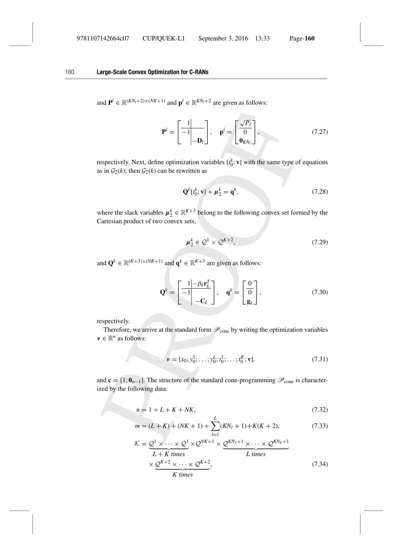
and Pl ∈ R(KNl+2)×(NK+1) and pl ∈ R

KNl+2 are given as follows:

Pl =⎡⎣ 1

−1−Dl

⎤⎦ , pl =⎡⎣

√Pl

00KNl

⎤⎦ , (7.27)

respectively. Next, define optimization variables [tk0; v] with the same type of equationsas in G2(k); then G2(k) can be rewritten as

Qk[tk0; v] + μk2 = qk, (7.28)

where the slack variables μk2 ∈ R

K+3 belong to the following convex set formed by theCartesian product of two convex sets,

μk2 ∈ Q1 × QK+2, (7.29)

and Qk ∈ R(K+3)×(NK+1) and qk ∈ R

K+3 are given as follows:

Qk =⎡⎣ 1 −βkrT

k−1

−Ck

⎤⎦ , qk =⎡⎣ 0

0gk

⎤⎦ , (7.30)

respectively.Therefore, we arrive at the standard form Pcone by writing the optimization variables

ν ∈ Rn as follows:

ν = [x0; y10; . . . ; yL

0; t10; . . . ; tK0 ; v], (7.31)

and c = [1; 0n−1]. The structure of the standard cone-programming Pcone is character-ized by the following data:

n = 1 + L + K + NK, (7.32)

m = (L + K) + (NK + 1) +L∑

l=1

(KNl + 1)+K(K + 2), (7.33)

K = Q1 × · · · × Q1︸︷︷︸L + K times

×QNK+1 × QKN1+1 × · · · × QKNL+1︸︷︷︸L times

×QK+2 × · · · × QK+2︸︷︷︸K times

, (7.34)



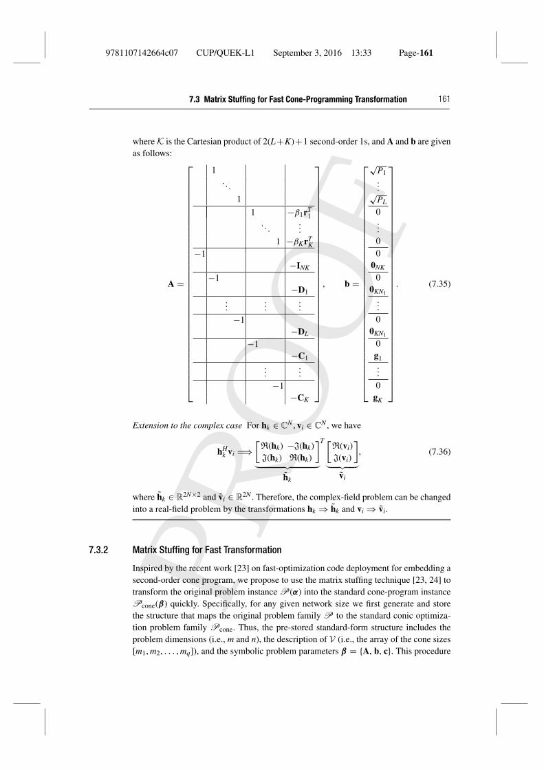
where K is the Cartesian product of 2(L+K)+1 second-order 1s, and A and b are givenas follows:

A =

⎡⎢⎢⎢⎢⎢⎢⎢⎢⎢⎢⎢⎢⎢⎢⎢⎢⎢⎢⎢⎢⎢⎢⎢⎢⎢⎢⎢⎢⎢⎢⎢⎢⎢⎢⎢⎢⎢⎣

1. . .

1

1 −β1rT1

. . ....

1 −βKrTK

−1−INK

−1−D1

......

...−1

−DL

−1−C1

......

−1−CK

⎤⎥⎥⎥⎥⎥⎥⎥⎥⎥⎥⎥⎥⎥⎥⎥⎥⎥⎥⎥⎥⎥⎥⎥⎥⎥⎥⎥⎥⎥⎥⎥⎥⎥⎥⎥⎥⎥⎦

, b =

⎡⎢⎢⎢⎢⎢⎢⎢⎢⎢⎢⎢⎢⎢⎢⎢⎢⎢⎢⎢⎢⎢⎢⎢⎢⎢⎢⎢⎢⎢⎢⎢⎢⎢⎢⎢⎢⎢⎣

√P1...√PL

0...00

0NK

00KN1

...0

0KN1

0g1...0

gK

⎤⎥⎥⎥⎥⎥⎥⎥⎥⎥⎥⎥⎥⎥⎥⎥⎥⎥⎥⎥⎥⎥⎥⎥⎥⎥⎥⎥⎥⎥⎥⎥⎥⎥⎥⎥⎥⎥⎦

. (7.35)

Extension to the complex case For hk ∈ CN , vi ∈ C

N , we have

hHk vi =⇒

[R(hk) −J(hk)J(hk) R(hk)

]︸︷︷︸

hk

T [R(vi)J(vi)

]︸︷︷︸

vi

, (7.36)

where hk ∈ R2N×2 and vi ∈ R

2N . Therefore, the complex-field problem can be changedinto a real-field problem by the transformations hk ⇒ hk and vi ⇒ vi.

7.3.2 Matrix Stuffing for Fast Transformation

Inspired by the recent work [23] on fast-optimization code deployment for embedding asecond-order cone program, we propose to use the matrix stuffing technique [23, 24] totransform the original problem instance P(α) into the standard cone-program instancePcone(β) quickly. Specifically, for any given network size we first generate and storethe structure that maps the original problem family P to the standard conic optimiza-tion problem family Pcone. Thus, the pre-stored standard-form structure includes theproblem dimensions (i.e., m and n), the description of V (i.e., the array of the cone sizes[m1, m2, . . . , mq]), and the symbolic problem parameters β = {A, b, c}. This procedure



can be done offline. Furthermore, to reduce the storage and memory overhead we storethe problem data β in a sparse form [43] by storing only the non-zero entries.

Using the pre-stored structure, for a given problem instance P(α) we need only copyits parameters α to the corresponding problem data β in the standard conic-optimizationproblem family Pcone. As the procedure for transformation needs only to copy memory,it thus is suitable for fast transformation and can avoid repeated parsing and generatingas in parser/solver modeling frameworks like CVX [21] and YALMIP [22].

Example 7.5 Matrix stuffing for the coordinated beamforming problem For theconvex coordinated beamforming problem (7.16), to arrive at the standard cone programform Pcone(β), we need only copy the parameters of the transmit power constraints Pl

to the data of the standard form, i.e., for the√

Pl in b, copy the parameters of the SINRthresholds γ to the data of the standard form, i.e., the βk in A, and copy the parametersof the channel realizations hk to the data of the standard form, i.e., the rk and Ck in A.As we need to copy the memory only for the transformation, this procedure can be veryefficient compared with state-of-the-art numerical-based modeling frameworks such asCVX.

7.3.3 Practical Implementation Issues

We have presented a systematic way to equivalently transform the original problems P

to standard conic optimization problems Pcone. The resultant structure that maps theoriginal problem to the standard form can be stored and reused for fast transforming viamatrix stuffing. This can significantly reduce the modeling overhead compared with theparser/solver modeling frameworks such as CVX. However, it requires tedious manualwork to find the mapping, and it may not be easy to verify its correctness. Chu et al.[23] made an attempt that was intended to automatically generate the code for matrixstuffing. However, so far the corresponding software package QCML [23] is far fromcomplete and may not be suitable for our applications. Extending numerically basedtransformation modeling frameworks like CVX to symbolically based transformationmodeling frameworks like QCML is non-trivial and requires tremendous mathematicaland technical effort.

7.4 Operator Splitting for Large-Scale Homogeneous Self-Dual Embedding

Although the standard cone program Pcone itself is suitable for parallel computing viathe operator splitting method [44], directly working on this problem may fail to providecertificates of infeasibility. To address this limitation, on the basis of the recent workby O’Donoghue et al. [45] we propose to solve the homogeneous self-dual embedding[34] of the primal–dual pair of the cone program Pcone. The resultant homogeneous


7.4 Operator Splitting for Large-Scale Homogeneous Self-Dual Embedding 163

self-dual embedding is further solved via the operator splitting method, also known asthe ADMM algorithm [27].

7.4.1 Homogeneous Self-Dual Embedding of Cone Programming

The basic idea of homogeneous self-dual embedding is to embed the primal and dualproblems of the cone program Pcone into a single feasibility problem (i.e., finding afeasible point of the intersection of a subspace and a convex set) such that either theoptimal solution or the certificate of infeasibility of the original cone program Pcone

can be extracted from the solution of the embedded problem.The dual problem of Pcone is given by [45]

Dcone : maximizeη,λ

−bTη

s. t. − ATη + λ = c,

(λ, η) ∈ {0}n × K∗, (7.37)

where λ ∈ Rn and η ∈ R

m are the dual variables and K∗ is the dual cone of the convexcone K. Define the optimal values of the primal program Pcone and dual program Dcone

as p� and d�, respectively. Let p� = +∞ and p� = −∞ indicate primal infeasibilityand unboundedness, respectively. Similarly, let d� = −∞ and d� = +∞ indicate dualinfeasibility and unboundedness, respectively. We assume strong duality for the convexcone program Pcone, i.e., p� = d�, including the cases when they are infinite. This is astandard assumption made when practically designing solvers for conic programs, e.g.,it is assumed in [17–19, 34, 45]. Besides this, we do not make any regularity assumptionon the feasibility and boundedness assumptions on the primal and dual problems.

Certificates of InfeasibilityGiven the cone program Pcone, a main task is to detect feasibility. However, most exist-ing custom algorithms assume that the original problem P is feasible [10] or provideheuristic ways to handle infeasibility [26]. Nevertheless, the only way to detect infeasi-bility effectively is to provide a certificate or proof of infeasibility, as presented in thefollowing proposition.

P RO P O S I T I O N 7.1 (Certificates of infeasibility) The following system,

Aν + μ = b, μ ∈ K, (7.38)

is infeasible if and only if the following system is feasible

ATη = 0, η ∈ K�, bTη < 0. (7.39)

Therefore, any dual variable η satisfying the system (7.39) provides a certificate or proofthat the primal program Pcone (equivalently, the original problem P) is infeasible.

Similarly, any primal variable ν satisfying the system

− Aν ∈ K, cTν < 0, (7.40)

is a certificate of the infeasibility of the dual program Dcone.



Proof This result follows directly from the theorem of strong alternatives [11, Section5.8.2].

Optimality ConditionsIf the transformed standard cone program Pcone is feasible then (ν�, μ�, λ�, η�) are opti-mal if and only if they satisfy the following Karush–Kuhn–Tucker (KKT) conditions:

Aν� + μ� − b = 0, (7.41)

ATη� − λ� + c = 0, (7.42)

(η�)Tμ� = 0, (7.43)

(ν�, μ�, λ�, η�) ∈ Rn × K × {0}n × K∗. (7.44)

In particular, the complementary slackness condition (7.43) can be rewritten as

cTν� + bTη� = 0, (7.45)

which explicitly forces the duality gap to be zero.

Homogeneous Self-Dual EmbeddingWe can first detect feasibility by Proposition 7.1 and then solve the KKT system ifthe problem is feasible and bounded. However, the disadvantage of such a two-phasemethod is that two related problems (i.e., checking feasibility and solving KKT con-ditions) need to be solved sequentially [34]. To avoid such inefficiency, we propose tosolve the following homogeneous self-dual embedding [34]:

Aν + μ − bτ = 0, (7.46)

ATη − λ + cτ = 0, (7.47)

cTν + bTη + κ = 0, (7.48)

(ν, μ, λ, η, τ , κ) ∈ Rn × K × {0}n × K∗ × R+ × R+, (7.49)

which embeds all the information on infeasibility and optimality into a single system byintroducing two new nonnegative variables τ and κ , which encode different outcomes.Thus the homogeneous self-dual embedding can be rewritten in the following compactform:

FHSD : find (x, y)

s. t. y = Qx,

x ∈ C, y ∈ C∗, (7.50)

where ⎡⎣λ

μ

κ

⎤⎦︸︷︷︸

y

=⎡⎣ 0 AT c

−A 0 b−cT −bT 0

⎤⎦︸︷︷︸

Q

⎡⎣ν

η

τ

⎤⎦︸︷︷︸

x

. (7.51)



In (7.51), x ∈ Rm+n+1, y ∈ R

m+n+1, Q ∈ R(m+n+1)×(m+n+1), C = R

n × K∗ × R+, andC∗ = {0}n × K × R+. This system has a trivial solution with all variables as zeros.

The homogeneous self-dual embedding problem FHSD is thus a feasibility problemfinding a non-zero solution in the intersection of a subspace and a convex cone. Let(ν, μ, λ, η, τ , κ) be a non-zero solution of the homogeneous self-dual embedding. Wethen have the following remarkable trichotomy, derived in [34]:

• Case 1, τ > 0, κ = 0, then

ν = ν/τ , η = η/τ , μ = μ/τ (7.52)

are the primal and dual solutions to the cone program Pcone.• Case 2, τ = 0, κ > 0; this implies that cTν + bTη < 0. Then

1. If bTη < 0 then η = η/(−bTη) is a certificate of primal infeasibility, as

AT η = 0, η ∈ V�, bT η = −1. (7.53)

2. If cTν < 0 then ν = ν/(−cT ν) is a certificate of dual infeasibility, as

− Aν ∈ V , cT ν = −1. (7.54)

• Case 3, τ = κ = 0; no conclusion can be made about the cone problem Pcone.

Therefore, from the solution to the homogeneous self-dual embedding, we can extracteither the optimal solution (based on (7.31)) or the certificate of infeasibility for theoriginal problem. Furthermore, as the set (7.49) is a Cartesian product of a finite numberof sets, this will enable parallelizable algorithm design. With these distinct advantagesof homogeneous self-dual embedding, in the sequel we focus on developing efficientalgorithms to solve the large-scale feasibility problem FHSD via the operator splittingmethod.

7.4.2 The Operator Splitting Method

Conventionally, the convex homogeneous self-dual embedding FHSD can be solvedvia the interior-point method, e.g. [17–19, 34]. However, the computational cost ofsuch a second-order method can still be prohibitive for large-scale problems. Instead,O’Donoghue et al. [45] developed a first-order optimization algorithm based on theoperator splitting method, i.e., the ADMM algorithm [27], to solve a large-scale homo-geneous self-dual embedding. The key observation is that the convex cone constraintin FHSD is the Cartesian product of smaller standard convex cones (i.e., second-order cones, semidefinite cones, and nonnegative reals), which enables parallelizablecomputing.

Specifically, the homogeneous self-dual embedding problem FHSD can be rewrittenas

minimize IC×C∗ (x, y) + IQx=y(x, y), (7.55)



where IS is the indicator function of the set S, i.e., IS (z) is zero for z ∈ S and +∞otherwise. By replicating the variables x and y, problem (7.55) can be transformed intothe following consensus form [27, Section 7.1]:

PADMM : minimize IC×C∗ (x, y) + IQx=y(x, y)

s. t. (x, y) = (x, y), (7.56)

which is readily solved by the operator splitting method.Applying the ADMM algorithm [27, Section 3.1] to the problem PADMM and elim-

inating the dual variables by exploiting the self-dual property of the problem FHSD

(refer to [45, Section 3] on how to simplify the ADMM algorithm), the final algorithmis obtained as follows:

OSADMM :

⎧⎪⎨⎪⎩x[i+1] = (I + Q)−1(x[i] + y[i]),x[i+1] = C(x[i+1] − y[i]),y[i+1] = y[i] − x[i+1] + x[i+1],

(7.57)

where C(x) denotes the Euclidean projection of x onto the set C. This algorithm hasan O(1/k) convergence rate [46] with k as the iteration counter (i.e., ε-accuracy can beachieved in O(1/ε) iterations) and will not converge to zero if a non-zero solution exists[45, Section 3.4]. Empirically, this algorithm can converge to modest accuracy within areasonable amount of time. As the last step is computationally trivial, in the sequel wewill focus on how to solve the first two steps efficiently.

7.4.3 Subspace Projection Algorithms

The first step in the algorithm OSADMM is a subspace projection. After simplifica-tion [45, Section 4], we essentially need to solve the following linear equation at eachiteration, i.e., [

I −AT

−A −I

]︸︷︷︸

S

[ν

−η

]︸︷︷︸

x

=[ν[i]

η[i]

]︸︷︷︸

b

, (7.58)

for the given ν[i] and η[i] at iteration i, where S ∈ Rd×d with d = m + n is a symmetric

quasidefinite matrix [47]. Several approaches will be presented to solve the large-scalelinear system (7.58) efficiently, i.e., so as to trade off the solving time and accuracy.

Factorization Caching ApproachTo enable quicker inversions and reduce memory overhead via exploiting the sparsity ofthe matrix S, the method of sparse permuted LDLT factorization [43] can be adopted.Specifically, such a factor-solve method can be carried out by first computing the sparsepermuted LDLT factorization as follows:

S = PLDLTPT , (7.59)

where L is a lower-triangular matrix, D is a diagonal matrix [44], and P with P−1 = PT

is a permutation matrix to fill in the factorization [43], i.e., the non-zero entries in L.



Such a factorization exists for any permutation P, as the matrix S is symmetric quasidef-inite [47, Theorem 2.1]. Computing the factorization costs much less than O(1/3d3)flops, while the exact value depends on d and the sparsity pattern of S in a complicatedway. Note that this factorization needs to be computed only once, in the first iteration,and can be cached for reusing in the sequent iterations for subspace projections. This iscalled the factorization caching technique [45].

Given the cached factorization (7.59), solving subsequent projections x = S−1b(7.58) can be carried out by solving the following much easier equations,

Px1 = b, Lx2 = x1, Dx3 = x2, LTx4 = x3, PTx = x4, (7.60)

which cost respectively zero flops, O(sd) flops by forward substitution with s as thenumber of non-zero entries in L, O(d) flops, O(sd) flops by backward substitution, andzero flops, respectively [11, Appendix C].

Approximate ApproachesTo scale the linear system (7.58) to large problem sizes for, approximate algorithms canbe adopted to trade off the accuracy of the solution and the solving time. We first rewrite(7.58) as follows:

ν = (I + ATA)−1(ν[i] − ATη[i]), (7.61)

η = η[i] + Aν. (7.62)

The conjugate gradient method [48] is then applied to find an approximation to the abovelinear system. Specifically, let G = I + ATA. The conjugate gradient algorithm to findx such that Gx = b is given by [48, Section 10.2]

βk = rTk−1rk−1/

(rT

k−2rk−2)

, (7.63)

pk = rk−1 + βkpk−1, (7.64)

αk = rTk−1rk−1/

(pT

k Gpk

), (7.65)

xk = xk−1 + αkpk, (7.66)

rk = rk−1 − αkGpk. (7.67)

This is used until the norm of the residual ‖rk‖2 is sufficiently small. As the iterationsonly require a matrix–vector multiplication operation, the conjugate gradient methodcan be very efficient. Other approximate approaches to solving the linear system (7.61),(7.62) can be found in [48]. The applicability of the approximate algorithms methodis based on the fact that if the subspace projection error is bounded by a summablesequence then the ADMM algorithm OSADMM will converge [45, 49].

7.4.4 Cone Projection

Proximal AlgorithmThe second step in the algorithm OSADMM is to project a point ω onto the cone C.As C is the Cartesian product of a finite number of smaller convex cones Ci, we canperform projection onto C by projecting onto Ci separately and in parallel. Furthermore,



the projection onto each convex cone can be done with closed forms. For example, fornonnegative real Ci = R+, we have that [50, Section 6.3.1]

Ci (ω) = ω+, (7.68)

where the nonnegative-part operator (·)+ is taken elementwise. For the second-ordercone Ci = {(y, x) ∈ R × R

p−1|‖x‖ ≤ y}, we have that [50, Section 6.3.2]

Ci (ω, τ ) =⎧⎨⎩

0, ‖ω‖2 ≤ −τ ,(ω, τ ), ‖ω‖2 ≤ τ

(1/2)(1 + τ/‖ω‖2)(ω, ‖ω‖2), ‖ω‖2 ≥ |τ |.(7.69)

For the semidefinite cone Ci = {X ∈ Rn×n|X = XT , X � 0}, we have that [50, Section

6.3.3]

Ci() =n∑

i=1

(λi)+uiuTi , (7.70)

where∑n

i=1 λiuiuTi is the eigenvalue decomposition of . More examples on the cone

projection (e.g., the exponential cone projection) can be found in [50].

Randomized AlgorithmsAlthough the cone projection can be performed in parallel with closed forms, the scalingmay be prohibitive on the semidefinite cone projection via eigenvalue decomposition.Therefore, to scale well to large problem sizes for SDP problems, it is of great interestto develop efficient algorithms to solve approximately the semidefinite cone projec-tion problem with rigorous performance and convergence guarantees for the resultingADMM algorithm OSADMM.

Randomized sketching provides powerful randomized and sampling techniques forlarge-scale matrices by compressing them into much smaller matrices, thereby savingsolving time and memory by reducing the problem dimensions. For semidefinite coneprojection, to project a symmetric matrix A ∈ R

n×n onto the positive semidefinite cone,we need to first perform its eigenvalue expansion and then drop the terms associated withnegative eigenvalues. The randomized algorithms for the eigenvalue decomposition ofthe symmetric matrix A ∈ R

n×n generally consist of the following simple steps [51]:

1. generate the orthonormal matrix Q ∈ Rm×n (m < n) such that ‖A − QQTA‖ ≤ ε

with ε as the computational tolerance;2. form the smaller matrix B = QAQT ;3. compute an eigenvalue decomposition B = V�VT ;4. form the orthonormal matrix U = QV such that A ≈ U�UT .

For step 1, several efficient randomized schemes were discussed in [51, Section 4]to minimize the sampling size and computational cost for producing the matrix Q. Asimple scheme is based on the Gaussian random matrix. In step 3, once we have B wecan adopt any of the standard deterministic factorization techniques in [51, Section 3.3]to produce eigenvalue decomposition. More efficient algorithms for factorization can



be found in [51, Section 5.2] by exploiting the information in Q. Typically, random-ized algorithms only require O(n2 log(k)) flops while classic algorithms require O(n2k)flops to do eigenvalue decomposition for a rank-k matrix A. More recent progress onrandomized sketching methods for numerical linear algebra can be found in [52, 53].

Although randomized algorithms can exploit randomness as a source for speedup,it is non-trivial to apply these algorithms directly for approximate cone projectionswith performance and convergence guarantees for the resulting operator splitting algo-rithm OSADMM. It is thus of great interest to establish theoretical guarantees for therandomized cone projection methods in the algorithm OSADMM.

7.4.5 Practical Implementation Issues

We have thus far presented the two-stage parallel computing framework for large-scaleconvex optimization in dense C-RANs. Here, we will discuss implementation issues ofthe proposed framework in C-RANs, thereby exploiting the computational architecturesto obtain further speed gains.

Parallel and Distributed ImplementationThe operator splitting algorithm OSADMM that we have presented is compact andparameter-free, with parallelizable computing and linear convergence. In particular,each iteration of the algorithm is simple and easy for parallel and distributed comput-ing. This allows the algorithm OSADMM to utilize the cloud computing environments inC-RANs with shared computing and memory resources in a single BBU pool. Specif-ically, the parallel algorithms can be leveraged in the subspace projection for LDLT

factorization and sparse matrix–vector multiplication [54]. The cone projection can beparallelized easily by projecting onto Ki separately and in parallel. However, it is chal-lenging to accommodate the operator splitting algorithm to the distributed environmentsin heterogeneous C-RANs [4, 8], Fog-RAN, and MENG-RAN [5]. In particular, mes-sage updates across the network (e.g., backhaul network) and synchronization amongheterogenous computation units will significantly increase the communication complex-ity in the distributed algorithms, which may result in delay and loss of performance.Therefore, it is critical to design large-scale distributed optimization algorithms with theminimal requirements of synchronization and communication.

Real-Time ImplementationIn dense C-RANs, to satisfy the strict low-latency demands, e.g., in Tactile Internet theend-to-end latency is constrained to one millisecond [55], we need to solve large-scaleoptimization problems in a millisecond. This brings significant challenges comparedwith large-scale optimization problems in machine learning and big data, where latencyis not a big issue but the problem dimension is often in the order of millions.

To solve a large-scale optimization problem in a real-time way, one promisingapproach is to leverage the symbolic subspace and cone projections. The general idea isto generate and store all the structures and descriptions of the algorithm for the specificproblem family Pcone. Eventually, the ADMM solver can be symbolically based so as



to provide numerical solutions for each problem instance Pcone(β) extremely quicklywithin a hard real-time deadline. This idea has already been successfully applied in thecode generation system CVXGEN [56] for real-time convex quadratic optimization [57]and in the interior-point based SOCP solver [58] for embedded systems. It is of greatinterest to implement this idea for the operator splitting algorithm OSADMM for generalreal-time conic optimization.

7.5 Numerical Results

In this section we simulate the proposed two-stage large-scale convex optimizationframework for performance optimization in dense C-RANs. The corresponding MAT-LAB code that can reproduce all the simulation results using the proposed large-scaleconvex optimization algorithm is available online.1

We considered the following channel model for the link between the kth MU and thelth RRH:

hkl = 10−L(dkl)/20√ϕklsklfkl, ∀k, l, (7.71)

where L(dkl) is the path loss in dB at distance dkl, as in [2, Table I], skl is the shad-owing coefficient, ϕkl is the antenna gain, and fkl is the small-scale fading coefficient.We used the standard cellular network parameters as in [2, Table I]. All the simulationswere carried out on a personal computer with a 3.2 GHz quad-core Intel Core i5 pro-cessor and 8 GB of RAM running Linux. The reference implementation of the operatorsplitting algorithm SCS is available online;2 it is a general software package for solv-ing large-scale convex cone problems based on [45] and can be called by the modelingframeworks CVX and CVXPY [59]. The settings (e.g., the stopping criteria) of SCS canbe found in [45].

The proposed two-stage approach framework, termed “Matrix Stuffing+SCS”, iscompared with the following state-of-the-art frameworks:

• CVX+SeDuMi/SDPT3/MOSEK This category adopts second-order methods. Themodeling framework CVX will first automatically transform the original probleminstance (e.g., the problem P written in disciplined convex programming form)into the standard cone-programming form and then call an interior-point solver, e.g.,SeDuMi [17], SDPT3 [18], or MOSEK [19].

• CVX+SCS In this framework based on first-order methods, CVX first transformsthe original problem instance into the standard form and then calls the operatorsplitting solver SCS.

We define the modeling time as the transformation time for the first stage, the solvingtime as the time spent on the second stage, and the total time as the time for the twostages to solve one problem instance. As the large-scale convex optimization algorithm

1 https://github.com/ShiYuanming/large-scale-convex-optimization2 https://github.com/cvxgrp/scs


7.5 Numerical Results 171

should scale well to both the modeling part and the solving part simultaneously, the timecomparison of each individual stage will demonstrate the effectiveness of the proposedtwo-stage approach.

Given the network size, we first generate and store the problem structure of the stan-dard conic optimization problem family Pcone, i.e., the structure of A, b, c, and thedescriptions of K. As this procedure can be done offline for all the candidate networksizes, we thus ignore this step for time comparison. The following procedures to solvethe large-scale convex optimization problem instances P(α) are repeated with differentparameters α and sizes using the proposed framework Matrix Stuffing+SCS:

1. Copy the parameters in the problem instance P(α) to the data in the pre-storedstructure of the standard cone program Pcone.

2. Solve the resultant standard conic optimization problem instance Pcone(β) using thesolver SCS.

3. Extract the optimal solutions of P(α) from the solutions to Pcone(β) produced bythe solver SCS.

Finally, note that all the interior-point solvers are multiple threaded (i.e., they canutilize multiple threads to gain extra speedups), while the operator splitting algorithmsolver SCS is single threaded. Nevertheless, we will show that SCS performs muchfaster than the interior-point solvers. We also emphasize that the operator splittingmethod is aimed to scale well to large problem sizes and thus to provide solutions tomodest accuracy within a reasonable time, while the interior-point method’s intendedto provide highly accurate solutions. Furthermore, the modeling framework CVX pro-vides rapid prototyping and a user-friendly tool for automatic transformations forgeneral problems, while the matrix-stuffing technique targets large-scale problems forthe specific problem family P . Therefore, these frameworks and solvers are not reallycomparable in view of their different purposes and application capabilities. We mainlyuse them to verify the effectiveness and reliability of our proposed framework in termsof solution time and solution quality.

7.5.1 Effectiveness and Reliability of the Large-Scale Optimization Framework

Consider a network with L two-antenna RRHs, K single-antenna MUs, and L = K,where all the RRHs and MUs are uniformly and independently distributed in the squareregion [−3000, 3000] × [−3000, 3000] meters. We consider the total transmit-powerminimization problem PSOCP with the objective function as ‖v‖2

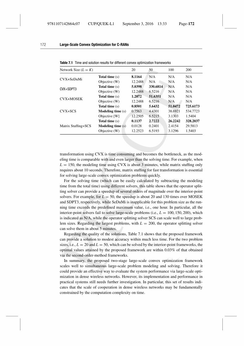
2 and the QoS require-ments for each MU as γk = 5 dB, ∀k. Table 7.1 demonstrates for comparison the runningtime and solutions using different convex optimization frameworks. Each point of thesimulation results is averaged over 100 randomly generated network realizations (i.e.,one small-scale fading realization for each large-scale fading realization).

For the modeling time comparisons, this table shows that the time value of theproposed matrix-stuffing technique ranges between 0.01 and 30 seconds for differentnetwork sizes and can bring a speedup of about 15 to 60 times compared with theparser/solver modeling framework CVX. In particular, for large-scale problems, the



Table 7.1 Time and solution results for different convex optimization frameworks

Network Size (L = K) 20 50 100 200

CVX+SeDuMiTotal time (s) 8.1164 N/A N/A N/AObjective (W) 12.2488 N/A N/A N/A

CVX+SDPT3Total time (s) 5.0398 330.6814 N/A N/AObjective (W) 12.2488 6.5216 N/A N/A

CVX+MOSEKTotal time (s) 1.2072 51.6351 N/A N/AObjective (W) 12.2488 6.5216 N/A N/A

CVX+SCSTotal time (s) 0.8501 5.6432 51.0472 725.6173Modeling time (s) 0.7563 4.4301 38.6921 534.7723Objective [W] 12.2505 6.5215 3.1303 1.5404

Matrix Stuffing+SCSTotal time (s) 0.1137 2.7222 26.2242 328.2037Modeling time (s) 0.0128 0.2401 2.4154 29.5813Objective (W) 12.2523 6.5193 3.1296 1.5403

transformation using CVX is time consuming and becomes the bottleneck, as the mod-eling time is comparable with and even larger than the solving time. For example, whenL = 150, the modeling time using CVX is about 3 minutes, while matrix stuffing onlyrequires about 10 seconds. Therefore, matrix stuffing for fast transformation is essentialfor solving large-scale convex optimization problems quickly.

For the solving time (which can be easily calculated by subtracting the modelingtime from the total time) using different solvers, this table shows that the operator split-ting solver can provide a speedup of several orders of magnitude over the interior-pointsolvers. For example, for L = 50, the speedup is about 20 and 130 times over MOSEKand SDPT3, respectively, while SeDuMi is inapplicable for this problem size as the run-ning time exceeds the predefined maximum value, i.e., one hour. In particular, all theinterior-point solvers fail to solve large-scale problems (i.e., L = 100, 150, 200), whichis indicated as N/A, while the operator splitting solver SCS can scale well to large prob-lem sizes. Regarding the largest problems, with L = 200, the operator splitting solvercan solve them in about 5 minutes.

Regarding the quality of the solutions, Table 7.1 shows that the proposed frameworkcan provide a solution to modest accuracy within much less time. For the two problemsizes, i.e., L = 20 and L = 50, which can be solved by the interior-point frameworks, theoptimal values attained by the proposed framework are within 0.03% of that obtainedvia the second-order-method frameworks.

In summary, the proposed two-stage large-scale convex optimization frameworkscales well to simultaneous large-scale problem modeling and solving. Therefore itcould provide an effective way to evaluate the system performance via large-scale opti-mization in dense wireless networks. However, its implementation and performance inpractical systems still needs further investigation. In particular, this set of results indi-cates that the scale of cooperation in dense wireless networks may be fundamentallyconstrained by the computation complexity on time.


7.5 Numerical Results 173

7.5.2 Max–Min Fairness Rate Optimization

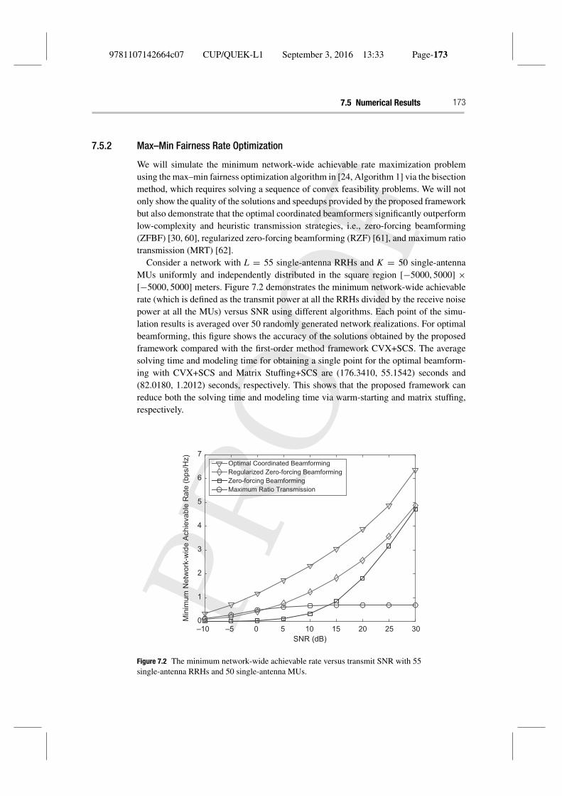
We will simulate the minimum network-wide achievable rate maximization problemusing the max–min fairness optimization algorithm in [24, Algorithm 1] via the bisectionmethod, which requires solving a sequence of convex feasibility problems. We will notonly show the quality of the solutions and speedups provided by the proposed frameworkbut also demonstrate that the optimal coordinated beamformers significantly outperformlow-complexity and heuristic transmission strategies, i.e., zero-forcing beamforming(ZFBF) [30, 60], regularized zero-forcing beamforming (RZF) [61], and maximum ratiotransmission (MRT) [62].

Consider a network with L = 55 single-antenna RRHs and K = 50 single-antennaMUs uniformly and independently distributed in the square region [−5000, 5000] ×[−5000, 5000] meters. Figure 7.2 demonstrates the minimum network-wide achievablerate (which is defined as the transmit power at all the RRHs divided by the receive noisepower at all the MUs) versus SNR using different algorithms. Each point of the simu-lation results is averaged over 50 randomly generated network realizations. For optimalbeamforming, this figure shows the accuracy of the solutions obtained by the proposedframework compared with the first-order method framework CVX+SCS. The averagesolving time and modeling time for obtaining a single point for the optimal beamform-ing with CVX+SCS and Matrix Stuffing+SCS are (176.3410, 55.1542) seconds and(82.0180, 1.2012) seconds, respectively. This shows that the proposed framework canreduce both the solving time and modeling time via warm-starting and matrix stuffing,respectively.

SNR (dB)

Min

imum

Net

wor

k-w

ide

Ach

ieva

ble

Rat

e (b

ps/H

z)

0–10 –5 0 5 10 15 20 25 30

1

2

3

4

5

6

7Optimal Coordinated BeamformingRegularized Zero-forcing BeamformingZero-forcing BeamformingMaximum Ratio Transmission

Figure 7.2 The minimum network-wide achievable rate versus transmit SNR with 55single-antenna RRHs and 50 single-antenna MUs.



Furthermore, this figure also shows that optimal beamforming can achieve quite animprovement for the per-user rate compared with the suboptimal transmission strategiesRZF, ZFBF, and MRT; this clearly shows the importance of developing optimal beam-forming algorithms for such networks. The average solving time and modeling time fora single point using CVX+SDPT3 for the RZF, ZFBF, and MRT are (2.6210, 30.2053)seconds, (2.4592, 30.2098) seconds, and (2.5966, 30.2161) seconds, respectively. Notethat the solving time is very small, because we only need to solve a sequence of lin-ear programming problems for power control when the directions of the beamformersare fixed during the bisection search procedure. The main time-consuming part is thetransformation using CVX.

7.6 Summary and Discussion

In this chapter we have presented a unified two-stage framework for large-scale opti-mization in dense C-RANs. We showed that various performance optimization problemsin C-RANs can be essentially solved by solving one, or a sequence of, convex opti-mization or convex feasibility problems. The proposed framework requires only theconvexity of the underlying problems without any other structural assumptions, e.g.,smooth or separable functions. This is achieved by first transforming the original convexproblem to a standard form via matrix stuffing and then using the ADMM algorithm tosolve the homogeneous self-dual embedding of the primal–dual pair of the transformedstandard cone program. Simulation results demonstrate the infeasibility detection capa-bility, the modeling flexibility and computing scalability, as well as the reliability of theproposed framework.

In principle one may apply the proposed framework to any large-scale convex opti-mization problem; one needs only to focus on the standard conic optimization formreformulation as well as to compute the proximal operators for different cone projec-tions. However, in practice the following issues need to be addressed in order to providea user-friendly framework and to assist practical implementation.

1. Developing a software package automatically generating the code for matrix stuffingis desirable but challenging in terms of reliability and correctness verification.

2. Efficient subspace and cone projection algorithms are highly desirable. In partic-ular, the randomized algorithms may provide a powerful method to scale up theprojections at each iteration, thereby trading off the solving time and the accuracyof solutions.

3. It is of great interest to implement the proposed large-scale convex optimizationframework in C-RANs by exploiting parallel and distributed computation archi-tectures, thereby further investigating the feasibility of this approach for real-timeapplications with strict low-latency requirements in wireless networks.

4. It is also of interest apply the proposed framework to various non-convex optimiza-tion problems, e.g., optimization on manifolds [63, 64].


References 175

References

[1] China Mobile, “C-RAN: the road towards green RAN,” White Paper, ver. 3.0, December2013.

[2] Y. Shi, J. Zhang, and K. B. Letaief, “Group sparse beamforming for green Cloud-RAN,”IEEE Trans. Wireless Commun., vol. 13, no. 5, pp. 2809–2823, May 2014.

[3] F. Bonomi, R. Milito, P. Natarajan, and J. Zhu, “Fog computing: a platform for inter-net of things and analytics,” in Big Data and Internet of Things: A Roadmap for SmartEnvironments, Springer International Publishing, 2014, pp. 169–186.

[4] M. Peng, Y. Li, J. Jiang, J. Li, and C. Wang, “Heterogeneous cloud radio access networks:a new perspective for enhancing spectral and energy efficiencies,” IEEE Wireless Commun.Mag., vol. 21, no. 6, pp. 126–135, December 2014.

[5] Y. Shi, J. Zhang, K. Letaief, B. Bai, and W. Chen, “Large-scale convex optimization forultra-dense cloud-ran,” IEEE Wireless Commun. Mag., vol. 22, no. 3, pp. 84–91, June 2015.

[6] A. B. Gershman, N. D. Sidiropoulos, S. Shahbazpanahi, M. Bengtsson, and B. Ottersten,“Convex optimization-based beamforming: from receive to transmit and network designs,”IEEE Signal Process. Mag, vol. 27, no. 3, pp. 62–75, 2010.

[7] Z.-Q. Luo, W.-K. Ma, A.-C. So, Y. Ye, and S. Zhang, “Semidefinite relaxation of quadraticoptimization problems,” IEEE Signal Process. Mag., vol. 27, no. 3, pp. 20–34, May 2010.

[8] E. Björnson and E. Jorswieck, “Optimal resource allocation in coordinated multi-cellsystems,” Found. Trends Commun. Inf. Theory, vol. 9, nos. 2–3, pp. 113–381, January 2013.

[9] D. P. Palomar and Y. C. Eldar, Convex Optimization in Signal Processing and Communica-tions. Cambridge University Press, 2010.

[10] H. Dahrouj and W. Yu, “Coordinated beamforming for the multicell multi-antenna wirelesssystem,” IEEE Trans. Wireless Commun., vol. 9, no. 5, pp. 1748–1759, September 2010.

[11] S. P. Boyd and L. Vandenberghe, Convex Optimization. Cambridge University Press, 2004.[12] R. Zakhour and S. V. Hanly, “Base station cooperation on the downlink: large system

analysis,” IEEE Trans. Inf. Theory, vol. 58, no. 4, pp. 2079–2106, April 2012.[13] C. Shen, T.-H. Chang, K.-Y. Wang, Z. Qiu, and C.-Y. Chi, “Distributed robust multicell

coordinated beamforming with imperfect CSI: an ADMM approach,” IEEE Trans. SignalProcess., vol. 60, no. 6, pp. 2988–3003, June 2012.

[14] Y. Shi, J. Zhang, and K. Letaief, “Robust group sparse beamforming for multicast greencloud-ran with imperfect csi,” IEEE Trans. Signal Process., vol. 63, no. 17, pp. 4647–4659,September 2015.

[15] J. Cheng, Y. Shi, B. Bai, W. Chen, J. Zhang, and K. Letaief, “Group sparse beamformingfor multicast green Cloud-RAN via parallel semidefinite programming,” IEEE Int. Conf.Communications, London, 2015.

[16] Y. Shi, J. Zhang, and K. Letaief, “Optimal stochastic coordinated beamforming for wirelesscooperative networks with CSI uncertainty,” IEEE Trans. Signal Process., vol. 63, no. 4, pp.960–973, February 2015.

[17] J. F. Sturm, “Using SeDuMi 1.02, a MATLAB toolbox for optimization over symmetriccones,” Optim. Methods Softw., vol. 11, no. 1–4, pp. 625–653, 1999.

[18] K.-C. Toh, M. J. Todd, and R. H. Tütüncü, “SDPT3 – a MATLAB software package forsemidefinite programming, version 1.3,” Optim. Methods Softw., vol. 11, nos. 1–4, pp. 545–581, 1999.



[19] E. D. Andersen and K. D. Andersen, “The mosek interior point optimizer for linearprogramming: an implementation of the homogeneous algorithm,” in High PerformanceOptimization, Springer, 2000, pp. 197–232.

[20] Y. Nesterov, A. Nemirovskii, and Y. Ye, Interior-Point Polynomial Algorithms in ConvexProgramming. SIAM, 1994, vol. 13.

[21] CVX Research, Inc., “CVX: Matlab software for disciplined convex programming, version2.0 (beta),” 2013. Online. Available at http://cvxr.com/cvx/

[22] J. Lofberg, “YALMIP: a toolbox for modeling and optimization in MATLAB,” in Proc.IEEE Int. Symp. Computer-Aided Control Systems Design, Taipei, September 2004, pp.284–289.

[23] E. Chu, N. Parikh, A. Domahidi, and S. Boyd, “Code generation for embedded second-ordercone programming,” in Proc. 2013 European Control Conf., July 2013, pp. 1547–1552.

[24] Y. Shi, J. Zhang, and K. Letaief, “Scalable coordinated beamforming for dense wire-less cooperative networks,” in Proc. IEEE Global Communications Conf., Austin, TX,December 2014, pp. 3603–3608.

[25] E. Bjornson, M. Bengtsson, and B. Ottersten, “Optimal multiuser transmit beamforming:a difficult problem with a simple solution structure [lecture notes],” IEEE Signal Process.Mag., vol. 31, no. 4, pp. 142–148, July 2014.

[26] W.-C. Liao, M. Hong, Y.-F. Liu, and Z.-Q. Luo, “Base station activation and lineartransceiver design for optimal resource management in heterogeneous networks,” IEEETrans. Signal Process., vol. 62, no. 15, pp. 3939–3952, August 2014. Online. Availableat http://arxiv.org/abs/1309.4138

[27] S. Boyd, N. Parikh, E. Chu, B. Peleato, and J. Eckstein, “Distributed optimization and sta-tistical learning via the alternating direction method of multipliers,” Found. Trends Mach.Learn., vol. 3, no. 1, pp. 1–122, July 2011.

[28] S. K. Joshi, M. Codreanu, and M. Latva-aho, “Distributed resource allocation for MISOdownlink systems via the alternating direction method of multipliers,” EURASIP J. WirelessCommun. Netw., vol. 2014, no. 1, pp. 1–19, January 2014.

[29] J. Zhang, R. Chen, J. G. Andrews, A. Ghosh, and R. W. Heath, “Networked MIMO withclustered linear precoding,” IEEE Trans. Wireless Commun., vol. 8, no. 4, pp. 1910–1921,April 2009.

[30] T. Yoo and A. Goldsmith, “On the optimality of multiantenna broadcast scheduling usingzero-forcing beamforming,” IEEE J. Sel. Areas Commun., vol. 24, no. 3, pp. 528–541,March 2006.

[31] Y. Shi, J. Zhang, B. O’Donoghue, and K. Letaief, “Large-scale convex optimization fordense wireless cooperative networks,” IEEE Trans. Signal Process., vol. 63, no. 18, pp.4729–4743, September 2015.

[32] E. Smith, “On the optimal design of continuous processes,” Ph.D. thesis, Imperial CollegeLondon (University of London), 1996.

[33] M. C. Grant and S. P. Boyd, “Graph implementations for nonsmooth convex programs,” inRecent Advances in Learning and Control, Springer, 2008, pp. 95–110.

[34] Y. Ye, M. J. Todd, and S. Mizuno, “An O(√

nL)-iteration homogeneous and self-dual linearprogramming algorithm,” Math. Oper. Res., vol. 19, no. 1, pp. 53–67, 1994.

[35] A. Wiesel, Y. Eldar, and S. Shamai, “Linear precoding via conic optimization for fixedMIMO receivers,” IEEE Trans. Signal Process., vol. 54, no. 1, pp. 161–176, January 2006.


References 177

[36] Y. Shi, J. Zhang, and K. Letaief, “Group sparse beamforming for green cloud radio accessnetworks,” in Proc. IEEE Global Communications Conf., Atlanta, GA, December 2013, pp.4635–4640.

[37] N. Jindal and A. Lozano, “A unified treatment of optimum pilot overhead in multipath fadingchannels,” IEEE Trans. Commun., vol. 58, no. 10, pp. 2939–2948, October 2010.

[38] D. J. Love, R. W. Heath, V. K. Lau, D. Gesbert, B. D. Rao, and M. Andrews, “An overviewof limited feedback in wireless communication systems,” IEEE J. Sel. Areas Commun.,vol. 26, no. 8, pp. 1341–1365, October 2008.

[39] M. A. Maddah-Ali and D. Tse, “Completely stale transmitter channel state information isstill very useful,” IEEE Trans. Inf. Theory, vol. 58, no. 7, pp. 4418–4431, July 2012.

[40] J. Zhang, R. W. Heath, M. Kountouris, and J. G. Andrews, “Mode switching for the multi-antenna broadcast channel based on delay and channel quantization,” Proc. EURASIP Conf.,J. Adv. Signal Process, Special Issue on Multiuser Lim. Feedback, vol. 2009, Article ID802548, 15 pp., 2009.

[41] E. Björnson, G. Zheng, M. Bengtsson, and B. Ottersten, “Robust monotonic optimizationframework for multicell MISO systems,” IEEE Trans. Signal Process., vol. 60, no. 5, pp.2508–2523, May 2012.

[42] L. J. Hong, Y. Yang, and L. Zhang, “Sequential convex approximations to joint chanceconstrained programs: a Monte Carlo approach,” Oper. Res., vol. 59, no. 3, pp. 617–630,May–June 2011.

[43] T. A. Davis, Direct Methods for Sparse Linear Systems. Societyfor Industrial and Applied Mathematics, 2006. Online. Available athttp://epubs.siam.org/doi/abs/10.1137/1.9780898718881.

[44] E. Chu, B. O’Donoghue, N. Parikh, and S. Boyd, “A primal–dual oper-ator splitting method for conic optimization,” 2013. Online. Available atwww.stanford.edu/ boyd/papers/pdos.html.

[45] B. O’Donoghue, E. Chu, N. Parikh, and S. Boyd, “Conic optimization via oper-ator splitting and homogeneous self-dual embedding,” 2013. Online. Available atarxiv.org/abs/1312.3039.

[46] T. Goldstein, B. O’Donoghue, S. Setzer, and R. Baraniuk, “Fast alternating direction opti-mization methods,” SIAM J. Imaging Sci., vol. 7, no. 3, pp. 1588–1623, 2014. Online.Available at dx.doi.org/10.1137/120896219.

[47] R. Vanderbei, “Symmetric quasidefinite matrices,” SIAM J. Optim., vol. 5, no. 1, pp. 100–113, 1995. Online. Available at dx.doi.org/10.1137/0805005.

[48] G. H. Golub and C. F. Van Loan, Matrix Computations. Johns Hopkins University Press,2012, vol. 3.

[49] J. Eckstein and D. P. Bertsekas, “On the douglas–rachford splitting method and the proximalpoint algorithm for maximal monotone operators,” Math. Progr., vol. 55, no. 1-3, pp. 293–318, 1992.

[50] N. Parikh and S. Boyd, “Proximal algorithms,” Found. Trends Optim., vol. 1, no. 3, January2014. Online. Available at www.stanford.edu/ boyd/papers.

[51] N. Halko, P.-G. Martinsson, and J. A. Tropp, “Finding structure with randomness: prob-abilistic algorithms for constructing approximate matrix decompositions,” SIAM Review,vol. 53, no. 2, pp. 217–288, 2011.

[52] M. W. Mahoney, “Randomized algorithms for matrices and data,” Found.Trends Mach. Learn., vol. 3, no. 2, pp. 123–224, 2011. Online. Available atdx.doi.org/10.1561/2200000035.



[53] D. P. Woodruff, “Sketching as a tool for numerical linear algebra,” Found. TrendsTheoret. Computer Sci., vol. 10, no. 1-2, pp. 1–157, 2014. Online. Available atdx.doi.org/10.1561/0400000060.

[54] J. Poulson, B. Marker, R. A. van de Geijn, J. R. Hammond, and N. A. Romero, “Elemental:a new framework for distributed memory dense matrix computations,” ACM Trans. Math.Softw., vol. 39, no. 2, p. 13, February 2013.

[55] G. Fettweis, “The tactile internet: applications and challenges,” IEEE Veh. Technol. Mag.,vol. 9, no. 1, pp. 64–70, March 2014.

[56] J. Mattingley and S. Boyd, “CVXGEN: a code generator for embedded convex optimiza-tion,” Optim. Engineering, vol. 13, no. 1, pp. 1–27, 2012.

[57] J. Mattingley and S. Boyd, “Real-time convex optimization in signal processing,” IEEESignal Process. Mag, vol. 27, no. 3, pp. 50–61, May 2010.

[58] A. Domahidi, E. Chu, and S. Boyd, “ECOS: an SOCP solver for embedded systems,” inProc. 2013 European Control Conf., IEEE, 2013, pp. 3071–3076.

[59] S. Diamond, E. Chu, and S. Boyd, “CVXPY: A Python-embedded modeling language forconvex optimization, version 0.2,” May 2014.

[60] J. Zhang and J. G. Andrews, “Adaptive spatial intercell interference cancellation in multicellwireless networks,” IEEE J. Sel. Areas Commun., vol. 28, no. 9, pp. 1455–1468, December2010.

[61] C. B. Peel, B. M. Hochwald, and A. L. Swindlehurst, “A vector-perturbation techniquefor near-capacity multiantenna multiuser communication – Part I: channel inversion andregularization,” IEEE Trans. Commun., vol. 53, no. 1, pp. 195–202, January 2005.

[62] F. Rusek, D. Persson, B. K. Lau, E. Larsson, T. Marzetta, O. Edfors et al., “Scaling upMIMO: opportunities and challenges with very large arrays,” IEEE Signal Process. Mag.,vol. 30, no. 1, pp. 40–60, January 2013.

[63] P.-A. Absil, R. Mahony, and R. Sepulchre, Optimization Algorithms on Matrix Manifolds.Princeton University Press, 2009.

[64] Y. Shi, J. Zhang, and K. B. Letaief, “Low-rank matrix completion via Riemannian pursuitfor topological interference management,” in Proc. IEEE Int. Symp. on Information Theory,Hong Kong, 2015.

7 large-scale convex optimization for c-ransfaculty.sist.shanghaitech.edu.cn/faculty/shiym/... · 7...

Documents