649 - ecmwf · 649 a new prognostic bulk microphysics scheme for the ifs richard m. forbes1, adrian...

649

A new prognostic bulk microphysicsscheme for the IFS

Richard M. Forbes1, Adrian M. Tompkins2

and Agathe Untch1

Research Department

1ECMWF 2ICTP, Italy

September 2011

Series: ECMWF Technical Memoranda

A full list of ECMWF Publications can be found on our web site under:http://www.ecmwf.int/publications/

Contact: [email protected]

c©Copyright 2011

European Centre for Medium-Range Weather ForecastsShinfield Park, Reading, RG2 9AX, England

Literary and scientific copyrights belong to ECMWF and are reserved in all countries. This publicationis not to be reprinted or translated in whole or in part without the written permission of the Director-General. Appropriate non-commercial use will normally be granted under the condition that referenceis made to ECMWF.

The information within this publication is given in good faith and considered to be true, but ECMWFaccepts no liability for error, omission and for loss or damage arising from its use.

http://www.ecmwf.int/publications/

New prognostic microphysics in the IFS

Abstract

A major upgrade to the parametrization of stratiform cloud and precipitation was implemented in theIntegrated Forecast System (IFS) Cycle 36r4, operational at ECMWF from 9 November 2010. Threeadditional prognostic variables have been introduced to enable a more physically based representa-tion of mixed-phase (liquid/ice) cloud and precipitating rain and snow. A fully implicit method isemployed to solve the network of microphysics pathways stably for long timesteps. It is the mostsignificant change to the structure of the cloud parametrization since the Tiedtke scheme was intro-duced operationally in 1995. Many aspects of the model are systematically improved including theskill of precipitation forecasts, the spatial distribution of ice and snow in the troposphere, the physicalprocesses in mixed-phase cloud and the impact of cloud and precipitation on radiation.

1 Introduction

The Tiedtke cloud scheme, described fully inTiedtke(1993), has served the Integrated Forecast System(IFS) well since its implementation in 1995. The scheme represents clouds in terms of two prognos-tics parameters; the first describing the horizontal coverage of the grid box by cloud, and the secondrepresenting the mass mixing ratio of total cloud condensate, which is divided into separate liquid andice categories diagnostically according to temperature. The approach includes parametrizations of thesources and sinks of the prognostic cloud variables due to all the major generation and destruction pro-cesses, including convection and microphysics. On the introduction of the new scheme into operationsin 1995, the monitoring of total cloud cover relative to SYNOP observations showed a distinct reductionin the error.

The scheme has since been under continual development with many aspects of the scheme changed fromthe original code, including the numerical formulation andmodifications to microphysical source andsink terms. Improvements have been made to the representation of ice cloud microphysics, includingthe process of ice sedimentation (Jakob, 2000), and a novel parametrization was developed for the sub-grid precipitation coverage which improved the representation of precipitation evaporation/sublimation(Jakob and Klein, 2000). Subsequently the numerics were rewritten to treat all cloud processes in par-allel. These changes did not improve the vertical resolution sensitivity of the scheme, and thus morerecent changes rejected the exact, semi-implicit cloud water and cover equation solvers in favour of aforward-in-time, upstream implicit approach. This introduced a separate treatment of autoconversion ofice crystals to snow, and reverted to using a constant sedimentation velocity for ice crystals to avoid nu-merical shocks. This was supplemented by a new parametrization to allow ice supersaturated conditionsin the cloud-free part of the grid box (Tompkinset al., 2007). The modified Tiedtke cloud scheme, inconjunction with the data assimilation and underlying forecast model system, has performed competi-tively with other state-of-the-art forecast models for cloud property predictions (Illingworth et al., 2007;Bouniol et al., 2010).

Despite all the above developments, the basic structure of the cloud scheme has remained essentiallythe same, with one prognostic variable for cloud fraction and one prognostic variable for cloud conden-sate. With increasing emphasis on cloud and precipitation in NWP and increasing resolution of the IFSmodel, it was clear that a number of changes were required to enable the continued improvement of thescheme, both now and looking ahead for the future. Particular issues that needed to be addressed in-cluded precipitation advection, representation of mixed-phase cloud, numerical implementation and thephysical realism of the scheme. These issues are discussed in turn below to provide the motivation forthe developments described in this report.

Technical Memorandum No. 649 1


(i) Precipitation advection: Higher horizontal resolution and shorter timesteps mean the original diag-nostic assumptions for precipitation become less valid. The diagnostic approach assumes the time takenfor precipitation to fall from cloud to ground is small compared to the timestep of the model and thathorizontal advection can be neglected on the spatial scale of the model grid resolution. A prognosticrepresentation of precipitation is therefore required as the model resolution and timestep increase, par-ticularly for snow particles which have a lower density and slower terminal fall speed than raindrops.

(ii) Mixed-phase cloud: The diagnostic approach to the mixed phase, which partitions the cloud con-densate into liquid and ice according to temperature in the range 0◦C to -23◦C, means that both ice andsupercooled liquid are always present in cloud in this temperature regime and no liquid water is allowedat temperatures colder than -23◦C. The reality can be very different. For example in this sub-zero tem-perature range, emerging convective clouds are often all liquid, established frontal clouds often all iceand thin mid-level cloud often topped with a shallow supercooled liquid water layer with ice particlesprecipitating out below. Supercooled liquid water is observed down to temperatures of -30◦C and colder(Hoganet al., 2007). If the model is to begin to capture these aspects, then an additional degree offreedom is required with separate prognostic variables forliquid and ice condensate.

(iii) Numerical issues: The diagnostic mixed-phase approach also leads to a numberof unrealistic nu-merical artefacts in the formulation of the microphysical processes, leading to a discontinuity in icesupersaturation and autoconversion of ice to snow at the mixed-phase temperature threshold (-23◦C) anda lack of sedimentation of ice in the mixed phase. This significantly affects the physical representationand the spatial distribution of ice in the mixed-phase temperature range. In addition, the diagnostic ap-proach assumes a single saturation curve in the mixed phase varying from water saturation at 0◦C toice saturation at -23◦C. In reality different microphysical processes respond differently to ice saturationand water saturation, such as the deposition growth of ice crystals at the expense of water drops (theWegener-Bergeron-Findeisen mechanism).

(iv) Physical realism: The representation of cloud with just two variables leads to a number of simplifi-cations and approximations in the scheme. Additional degrees of freedom allow for a more physicallyrealistic representation of cloud and precipitation microphysics that can be verified with observations.

This document describes the recent developments to the cloud scheme (implemented in IFS Cycle 36r4)that changes from a single prognostic cloud condensate variable to four prognostic variables for cloudliquid, cloud ice, rain and snow (as well as cloud fraction) in order to address some of the issues above.Section 2 describes the new scheme in terms of changes to the numerical framework, to the microphysi-cal processes and to interactions with other parts of the model. Section 3 highlights some of the impactson aspects of the model performance and Section 4 provides a concluding summary. The Appendicesinclude technical details of the new prognostic field initialization and the diagnostic output that is avail-able.

2 Description of the new prognostic microphysics scheme

2.1 Overview

The new parametrization of stratiform cloud and precipitation increases the number of prognostic vari-ables from two (cloud fraction, cloud condensate) to five (cloud fraction, cloud liquid water, cloud ice,rain and snow). The philosophy of the original Tiedtke scheme is retained with regards to a prognosticcloud fraction and sources and sinks of all cloud variables due to the major generation and destruction

2 Technical Memorandum No. 649


Cloudwater/ice

Watervapour

Autoconversion

Condensation Evaporation

Cloudfraction

Evaporation

Surface Precipitation

a Previous cloud scheme b New cloud scheme

Precipitationrain/snow

Cloudice

Snow

Cloudwater

Rain

Watervapour

Surface Precipitation

Freezing – Melting

Autoconversion Collection

Autoconversion Collection

Freezing – Melting – Bergeron

Deposition Sublimation

Condensation Evaporation

Ev

ap

ora

tio

n

Su

blim

atio

n

Cloudfraction

Figure 1:Schematic of the IFS cloud scheme: (a) the Tiedtke scheme with three moisture related prog-nostic variables operational from 1995 to 2010 (before IFS Cy36r4) and (b) the new cloud scheme withsix moisture related prognostic variables (Cy36r4 onwards). Yellow boxes indicate prognostic variables.

processes, including detrainment from convection. However, water and ice clouds are now independent,addressing many of the issues identified above and allowing amore physically realistic representation ofsupercooled liquid water cloud. Rain and snow precipitation are also now able to precipitate with a deter-mined terminal fall speed and can be advected by the three-dimensional wind. A new multi-dimensionalimplicit solver is implemented for the numerical solution of the cloud and precipitation prognostic equa-tions. Figure1 shows a schematic to highlight the differences between the new and old parametrizationschemes. This section describes the numerical framework and revised microphysical processes in thenew scheme. Further details of the cloud and precipitation parametrization scheme can be found in Part4 of the IFS Documentation for Cycle 37r2 (www.ecmwf.int/research/ifsdocs/CY37r2).

2.2 Numerical framework

The new scheme is a multi-species prognostic microphysics scheme, withm= 5 prognostic equationsfor water vapour, cloud liquid water, rain, cloud ice and snow. The equation governing each prognosticcloud variable within the cloud scheme is

∂qx

∂ t= Sx +

1ρ

∂∂z

(ρVxqx) , (1)

whereqx is the specific water content for categoryx (x = 1 for cloud liquid droplets,x = 2 for rain, andso on),Sx is the net source or sink ofqx through microphysical processes, and the last term representsthe sedimentation ofqx with fall speedVx.

The solution to this set of equations uses the upstream approach. Writing the advection term in mass fluxform, collecting all fast processes (relative to a GCM timestep) into an implicit term (B) and leaving therest in an explicit term (~A), gives

qn+1x −qn

x

∆t= Ax +

m

∑y=1

Bxyqn+1y −

m

∑y=1

Byxqn+1x +

ρk−1Vxqn+1x,k−1−ρVxqn+1

x

ρ∆Z. (2)

for timestepn. The subscript “k−1” refers to a term calculated at the model level above the present levelk for which all other terms are being calculated. The matrixB (with termsBxx, Bxy, Byx) represents all



the implicit microphysical pathways such thatBxy > 0 represents a source ofqx and a sink ofqy. MatrixB is positive-definite off the diagonal, with zero diagonal terms sinceBxx = 0 by definition. Some terms,such as the creation of cloud through condensation resulting from adiabatic motion or diabatic heating,are more suitable for an explicit framework, and are retained in the explicit term~A.

Due to the cross-termsqn+1y , (2) is rearranged to give a straight forward matrix equation which can

be solved with standard methods (the scheme currently uses the LU decomposition method). As longas the solution method is robust, the choice for solution is not critical as the number of microphysicalprognostic equations is small (m= 5), in contrast to chemical models with typically O(100) species. Thesolution method is simplified by assuming the vertical advection terms due to convective subsidence andsedimentation act only in the downward direction, allowingthe solution to be conducted level by levelfrom the model top down. The vertical advection term only appears on the diagonal, thus the matrixequation for a 3-variable system is

1+ ∆t( V1∆Z +B21+B31) −∆tB12 −∆tB13

−∆tB21 1+ ∆t( V2∆Z +B12+B32) −∆tB23

−∆tB31 −∆tB32 1+ ∆t( V3∆Z +B13+B23)

·

qn+11

qn+12

qn+13

=

[qn

1 + ∆t

(A1 +

ρk−1V1qn+11,k−1

ρ∆Z

),qn

2 + ∆t

(A2 +


ρ∆Z

),qn

3 + ∆t

(A3 +


ρ∆Z

)]. (3)

There are some aspects that require attention. Firstly, although implicit terms are unable to reduce acloud category to zero, the explicit can, and often will, achieve this. Thus safety checks are requiredto ensure that all end-of-timestep variables remain positive definite, in addition to ensuring conserva-tion. Practically, to aid the conservation requirement, the explicit source and sink terms are thus alsogeneralised from a vector~A to a matrixA, thus

A =

A11 A21 A31

A12 A22 A32

A13 A23 A33

. (4)

whereAxy > 0 represents a source ofqx and a sink ofqy, andAyx = −Axy. Although this matrix approachinvolves a degree of redundancy, it is a simple method of ensuring conservation properties. The matrixdiagonalsAxx contain the ’external’ sources ofqx such as the cloud water detrainment terms from theconvection scheme.

In order to simultaneously guarantee conservation and positive-definite properties, the sum of all sinksfor a given variable are scaled to avoid negative values. This solution is not accurate, seen from theconsideration of the simple case of a variable in equilibrium, with a small initial value subjected to alarge source and an equal and opposing sink: the sink will be clipped first and the variable will increase.However, this is deemed preferable to any method that attempts to account for variable sources, whichmust invoke a sensitivity to the order in which the variablesare considered.

The impact on the temperature budget is calculated from the change in cloud variables due to eachprocess after the cloud scheme ’solver’ has been applied, and then collecting the terms together that areassociated with latent heating/cooling. With the fully implicit solver it is thus easier to use conservedvariables to govern the temperature budget; the scheme usesthe liquid water temperatureTL defined as:

TL = T −Lv

Cp(ql +qr)−

Ls

Cp(qi +qs). (5)



SincedTL/dt = 0, the temperature change is thus given by

∂T∂ t

=m

∑x=1

L(x)Cp

(∂qx

∂ t−Dqx −

1ρ

∂∂z

(ρVxqx)

)(6)

The first term on the right in the brackets is the rate of changeof speciesqx due toall processes, includingthe convective detrainment termDqx and the advective flux terms, which are then subtracted separatelysince they represent a netTL flux not associated with latent heating.

For the prognostic cloud fraction variable, denoted bya, there are no multi-dimensional dependencies,so a matrix approach is not required and Eq.2 simplifies to

an+1−an

∆t= A+Ban+1. (7)

whereA andB are the explicit and implicit source/sink terms for the cloud fraction.

2.3 Revised microphysics

The strategy for the implementation of the prognostic cloud/precipitation variables was to minimize thenumber of microphysical changes in the existing scheme in order to facilitate the transition to the newframework in the operational model. However, the separation of cloud condensate into liquid and iceprognostic variables clearly requires new microphysical processes to describe the transfer between differ-ent water phases in mixed-phase cloud (particularly nucleation and depositional growth of ice crystals).In addition, a number of other alterations to the microphysics are described here.

The numerics previously treated all cloud processes in parallel, but the new scheme treats some processesin a sequential manner. This was necessary to ensure that archived variables made physical sense. Forexample, if processes are treated contemporaneously, gridboxes could exist with only liquid cloud andno ice at temperatures close to -38◦C, since in this approach freshly nucleated liquid cloud droplets mustwait until the subsequent timestep before they are able to undergo the freezing process. Thus a first-guessvariable is introduced to update the status of variables dueto all explicit processes during the course ofthe scheme.

The formulation of the convective detrainment and subsidence, stratiform condensation and evaporation,and turbulent erosion terms remain essentially the same as in the previous version of the scheme. Eachof the new or modified physical process in the cloud scheme is discussed in turn below.

2.3.1 Ice crystal nucleation and ice supersaturation

Ice crystal nucleation is restricted to the homogeneous process, which is parametrized simply, withno attempt made to predict the ice number concentration (Ni) produced by the nucleation event. Theice nucleation occurs on short timescales and is very sensitive to the updraught velocity on the cloudscale, which can only be crudely estimated from GCM resolvedvariables (Lohmann and Karcher, 2002;Karcher and Lohmann, 2002).

To retain consistency with the supersaturation treatment of Tompkinset al.(2007), at temperatures below0◦C new cloud forms in any non-cloudy part of the grid box where the humidity exceeds either theminimum of the liquid water saturation specific humidity (qsl), or the critical vapour saturation mixingratio with respect to ice at which homogeneous ice nucleation initiates (Pruppacher and Klett, 1997;



Koopet al., 2000). For the latter threshold the empirical fit given byKarcher and Lohmann(2002) isadopted, as before, which is a function of temperature and ranges from 45% supersaturation atT = 235 Kto 67% atT = 190 K:

RHhomo= 2.583−T

207.8(8)

whereT is the temperature in Kelvin. At temperatures warmer than -38◦C the cloud formation over atimestep results entirely in liquid cloud, while below thisthreshold the liquid water or aqueous sulphatesolutes are assumed to freeze instantaneously and the process is a source for cloud ice.

For the case of pure ice cloud formation, the deposition process is considered to be sufficiently rapidrelative to the model time-step that it can be approximated by a diagnostic adjustment to exactly icesaturated conditions inside the cloud. This assumption is necessary, since to allow ice supersaturationboth within the pure ice cloud and in the clear sky environment would either require a separate prognosticvariable to monitor the evolution of the water vapour insidethe cloud, or a diagnostic assumption wouldhave to be used to divide the grid-mean humidity between the two regions, which can generate largeartificial horizontal sub-grid humidity fluxes (seeTompkinset al., 2007, for more detail). In any case,this assumption appears to be reasonably justified in a wide range of updraught situations by modelling ofthe homogeneous nucleation process (Khvorostyanov and Sassen, 1998). The obvious drawback is thatpure ice clouds may not exist in a subsaturated or supersaturated state, and no information concerningthe ice crystal number concentration is available.

The new scheme now allows ice supersaturation in the 0◦C to -23◦C temperature range which was notpossible in the previous scheme due to the diagnostic temperature dependent assumption for the liq-uid/ice split. Figure2 shows a relative humidity versus temperature diagram to highlight this aspectin the previous and new versions of the scheme. Grid box mean relative humidity and temperature forcloudy points where cloud fraction is greater than 10% are plotted. The distribution of points is pre-dominantly along the model saturation curve, which for the previous scheme follows water saturationfor temperatures above freezing, mixed liquid-ice saturation between 0◦C to -23◦C and then ice satura-tion at temperatures colder than this. The occurrence of subsaturated grid box mean relative humiditieshighlights the ability of the model to retain cloud when the clear air humidity is below 100% due to thesub-grid heterogeneity assumption and prognostic cloud fraction variable. In addition supersaturationwith respect to ice can occur in the clear air at temperaturescolder than -23◦C, but a discontinuity inice supersaturation is seen at this temperature threshold (Fig. 2b). In contrast, the new scheme allowssubsaturated states and ice supersaturated states in the clear air at all temperatures below 0◦C with noartificial discontinuity at -23◦C (Fig. 2c).

2.3.2 Ice crystal growth by deposition in mixed phase clouds

The scheme allows supercooled liquid water to exist at temperatures warmer than the homogeneousfreezing threshold of -38◦C. At temperatures colder than this water droplets are assumed to freeze in-stantaneously. When supercooled liquid and ice are coexistent, they are assumed to be well mixedand distributed uniformly through the cloud (seeRotstaynet al. (2000) for a discussion of alternativeassumptions). The ice crystals can then grow at the expense of the water droplets through the Wegener-Bergeron-Findeisen process. If water droplets are present, the ice crystals are in an environment supersat-urated with respect to ice and grow by deposition, reducing the water vapour and leading to subsaturationwith respect to water. Water droplets then evaporate and theprocess continues with ice growth until thewater droplets are completely evaporated. Thus in mixed phase clouds, the deposition process acts as asink of cloud liquid and a source of ice cloud.



(a)

(b) (c)

Figure 2:Distribution of relative humidity (with respect to water) for cloudy and partially cloudy gridpoints as a function of temperature for a typical model forecast, (a) relevant curves for the microphysicalprocesses in the model, (b) data from the old scheme with diagnostic mixed-phase showing the discon-tinuity at -23◦C, (c) data from the new scheme allowing ice supersaturationat all temperatures colderthan 0◦C.

FollowingPruppacher and Klett(1997) andRotstaynet al. (2000), the rate of growth of an ice crystal ofmassMi is:

dMi

dt=

4πC(Si −1)

α + β, (9)

whereC is the capacitance of the particle (related to the shape) andSi = e/esi is the saturation ratio withrespect to ice. Termsα andβ represent heat conduction and vapour diffusion respectively,

α =Ls

KaT

(Ls

RvT−1

)(10)

β =RvTχesi

(11)



whereKa is the heat conductivity of air andχ is the diffusivity of water vapour in air, which variesinversely with pressure asχ = 2.21/p. If the ice crystal number concentration isNi and the ice crystalsare assumed to be monodispersed with all particles having equal diameterDi and equal massMi (andtherefore also equal densityρi), then the cloud ice specific water contentqi = MiNi/ρ . If the air is atwater saturation, thenSi = (esl −esi)/esi, and from (9) the rate of change ofqi is

dqi

dt=

Ni

ρ4πC

(α + β )

(esl −esi)

esi. (12)

The capacitance termC assumes ice crystals are spherical (C = Di/2) whereDi = (6Mi/πρi)1/3. Elimi-

nation ofC from (12) then gives

dqi

dt= cs

vdq1/3i (13)

where

csvd =

(Ni

ρ

)2/3 7.8

ρ1/3i (α + β )

(esl −esi)

esi. (14)

The analytical treatment ofRotstaynet al. (2000) is used, which assumes the temperature dependentquantities in (14) can be approximated as constant through the timestep. The ice condensate amount attime t can then be calculated by integrating (13) with respect to time, giving

qti =

(23

csvd∆t +(qt−1

i )2/3)3/2

(15)

and the deposition rate becomes,Sdep= (qti −qt−1

i )/∆t.

In order to calculate the deposition rate, the ice crystal concentration is required for (14), assuming het-erogeneous ice nucleation has occurred in the supersaturated air. As stated earlier, no prognostic equationfor the ice crystal concentration is introduced, and thusNi in (14) is given diagnostically, assuming the airis at water saturation, according to theMeyerset al. (1992) deposition-condensation-freezing nucleationparametrization:

Ni = 1000exp[12.96(esl −esi)/esi−0.639] (16)

The ice crystal concentration has great uncertainty butMeyerset al. (1992) showed (16) correlated wellwith continuous-flow diffusion-chamber measurements across a range of temperatures and supersatura-tions.

To initiate the glaciation process, at each gridbox, a minimum ice mass mixing ratio is assumed of

qmini =

mi0Ni

ρ(17)

wheremi0 is the initial mass of an ice particle and is set to 10−12kg afterWilson and Ballard(1999).

Once the supercooled liquid water reservoir in the cloud is exhausted through the deposition process,there is a complication to consider. At the point the cloud becomes completely glaciated, the in-cloudvapour pressure is equal toesl. From this point the ice crystals would continue to grow by depositionof water vapour, until the in-cloud vapour pressure is reduced to the saturation value with respect to ice



-35 -30 -25 -20 -15 -10 -5 0 5 10

Temperature (°C)

0

0.2

0.4

0.6

0.8

1

Liq

uid

Wa

ter

Fra

ctio

n

0.5 1 2 5 10 20 50 100 %

Figure 3:Global percentage occurrence (for a given temperature) of the liquid water fraction of cloudcondensate for the previous diagnostic temperature-dependent mixed-phase scheme (solid black line)and the new prognostic ice/liquid scheme (shading) for a range of temperatures (on 10 January 2011).

(or an equilibrium value exceeding the saturation value in the presence of strong updraughts, see forexampleRen and Mackenzie, 2005). However, unlike the mixed phase situation, where the “memory”for the vapour reservoir is provided by the prognostic cloudliquid water variable, there is no memoryfor the water vapour content in the cloudy region of the gridbox in order to model the deposition processin glaciated clouds. So, the new cloud follows the same assumption as before for pure ice cloud (seeprevious subsection) and the deposition of the remaining water vapour in excess of ice saturation occurswithin a single timestep, bringing the cloud to exactly ice saturation.

To summarise, in mixed phase clouds with supercooled liquidwater present the cloud is assumed tobe exactly at saturation with respect to water (and therefore supersaturated with respect to ice), andwhen only ice is present, the cloud is assumed to be exactly atsaturation with respect to ice. However,supersaturation is permitted in the clear sky portion of a grid cell in all cases.

It is the process of deposition that largely determines the partition between liquid and ice in mixed phaseclouds in the scheme. Figure3 shows the partition between ice and liquid cloud for an integrationusing the new scheme compared to the default model. It is seenthat the ’S’ shape is reproduced fromobservations (e.g.Rotstaynet al., 2000). Compared to the default model which sets liquid water fractiondiagnostically to zero at -23◦C, there are more occurrences of liquid water at temperatures colder than thisthreshold. The mode of the distribution still approximately follows the temperature-dependent function,but variability is significantly increased. For example, 100% of cloud is all ice at -35◦C, 100% is allliquid at +10◦C, but at -10◦C the cloud can vary from all ice, through varying fractions of supercooledliquid water, to all water. There is no liquid water at temperatures colder than around -38◦C due tohomogeneous freezing and there is more occurrence of pure ice cloud at all temperatures below 0◦C.Small ice fractions (i.e. liquid water fractions just less than one) at temperatures greater than 0◦C are dueto the fact that ice is allowed to fall and takes a finite time tomelt.



2.3.3 Freezing and melting

A new microphysical pathway is added to treat the melting of ice into liquid, which was not requiredin the previous scheme due to the diagnostic liquid/ice assumption and lack of sedimentation in the 0◦Cto -23◦C temperature range. In addition, the process of freezing rain is included, which converts rainto snow due to the lack of a suitable, hail-like category. Forthe freezing of rain, the treatment is verysimple, with all rain freezing in a timestep if the temperature is below 0◦C, with a check to ensure that thetemperature does not increase above this threshold due to the latent heating of the process. The meltingof ice and snow are treated in a similar way to the diagnostic snow variable in the previous scheme,allowing the melting to cool the gridbox to 0◦C over a specified timescale. These processes are currentlytreated explicitly.

2.3.4 Sedimentation

The numerical formulation of the sedimentation process (falling hydrometeors due to gravity) followsthe forward-in-time upstream approach as in the previous version. The rain, snow and ice hydrometeorcategories are allowed to sediment.

With the potential for hydrometeors to settle through many model layers in a single timestep, using amass related fall speed formulation (Vx = F(qx)) can lead to numerical ’shocks’ when long timesteps arenecessary (e.g.Wacker and Seifert, 2001). Thus the fallspeeds are set to a constant (Vi0 = 0.15 m s−1,Vs0 = 1 m s−1, Vr0 = 4 m s−1) to avoid this. However, the fallspeed for ice and snow are adjusted toaccount for variations in temperature and pressure as derived byHeymsfield and Iaquinta(2000),

Vx = Vx0

(p

pfall

)−0.178( TTfall

)−0.394

(18)

wherepfall = 30000 Pa andTfall = 233 K.

Sedimentation of ice in the previous scheme was not active inthe 0◦C to -23◦C temperature range andwas gradually increased to 0.15 m s−1 at temperatures colder than -23◦C. Therefore the new scheme hasan additional sink of ice due to sedimentation in this temperature range that was not present before. Thisreduces the ice water content compared to the previous scheme (as shown in Section 3.2).

2.3.5 Autoconversion

There are two changes to the autoconversion treatment. Previously, the autoconversion of ice to snowonly operated in the pure ice phase (T<-23◦C) with all cloud condensate treated by the rain autoconver-sion process for temperatures warmer than this threshold. This temperature threshold approach was usedto minimize impact on the cloud scheme when the snow autoconversion was introduced along with theimplicit numerical approach in Cycle 31r1. The surface precipitation and model hydrological cycle isvery sensitive to the treatment of the autoconversion in themixed phase, since the collection-term (rainand snow collecting cloud droplets) make the scheme highly nonlinear.

With separate cloud liquid and ice variables, there is no need to retain this artificial temperature thresholdin the new scheme, and now the snow autoconversion works to convert ice to precipitating snow, irre-spective of temperature, and the warm-phase autoconversion only takes liquid cloud into account. Theadjustment factor (Sundqvist, 1978) that accounts for the Bergeron-Findeisen process is also removed asthis process is now represented explictly by the depositionterm described above.



The rate of generation of precipitation is written as

Srainauto= ac0qcld

l

[1−exp

{−

(qcld

l

qcritl

)2}](19)

whereqcldl is the in-cloud value of cloud water content (ql/a), a is the cloud fraction,c−1

0 represents acharacteristic time scale for conversion of cloud liquid droplets into rain drops andqcrit

l is a typical cloudwater content at which the generation of precipitation begins to be efficient. The critical liquid watercontent is different over ocean and land to take account of the differences in cloud condensation nuclei(CCN) in clean and polluted air. Cleaner air over the ocean has fewer CCN, hence larger drops and anonset of precipitation at lower cloud liquid water contentsthan in the more polluted air over land. Thesetwo disposable parameters are defined as

c0 = c∗0F1 (20)

and

qcritl =

qcrit∗l

F1(21)

to take into account the effect of collection (accretion) ofcloud droplets by raindrops falling through thecloud (F1). HereF1 is defined as

F1 = 1+b1

√Ploc (22)

wherePloc is the local cloudy precipitation rate (Ploc = Pcld/acldP ) andacld

P is the precipitation fractionoverlapping with cloud (see section on precipitation below). For warm-phase autoconversion, the ratecoefficient isc∗0 = 1.67× 10−4 s−1 and the critical water contentqcrit∗

l is set to 3× 10−4 kg kg−1 overocean and 5×10−4 kg kg−1 over land. For cold-phase (ice to snow) autoconversion, therate coefficient(c0) is based onLin et al. (1983), c0 = 10−3e0.025(T−273.15) and the critical ice water contentqcrit

i is set to4×10−5kg kg−1.

The critical threshold is a factor of ten smaller for the cold-phase autoconversion and the autoconversionrate is a factor of 5 higher, so this change results in a much more efficient sink of ice cloud and thereforea significant decrease in the cloud ice contents is expected in the 0 to -23◦C temperature range (as shownin Section 3.2).

2.3.6 Precipitation evaporation/sublimation

Precipitation processes are treated separately in clear and cloudy skies. The microphysical processes inthese two regions are very distinct from each other, with conversion, collection and accretion processesbeing relevant in clouds whereas evaporation of precipitation is the relevant process outside clouds.

Whereas cloud fraction (for cloud liquid and cloud ice) is a prognostic variable, precipitation fraction (forrain and snow) is still treated diagnostically. The treatment of precipitation fraction in the previous cloudscheme (Jakob and Klein, 2000) in IFS cycles prior to 36r4 needed to be updated for the new prognosticmicrophysical treatment, since snow and rain water contentare now prognostic variables and can survivefrom one timestep to the next. So the previous complex two-stream treatment is replaced by a simplertreatment where the total precipitation fractionaP (the sum of the in-cloud precipitation fractionacld

P andthe clear sky precipitation fractionaclr

P ) is calculated using a maximum-random overlap treatment ofthecloud fraction, so that at levelk:

aP,k = 1−

((1−aP,k)(1−MAX[ak,ak−1])

1−MIN[ak−1,1− ε ]

), (23)



whereε is equal to a small number (10−6) andak is the cloud cover at levelk. The clear sky precipitationfraction is then given by

aclrP = aP−a. (24)

The precipitation flux is proportionally divided between the clear-sky and the in-cloud component, im-plying a greater artificial subgrid horizontal flux than in the previous diagnostic scheme. However, this isunavoidable without additional prognostic variables to represent the clear-sky and in-cloud precipitationcoverages.

For the evaporation process, the previous scheme assumed horizontal homogeneity of the precipitation.Thus in a sub-cloud layer the clear sky precipitation fraction (aclr

P ) remained constant while the fluxreduced due to evaporation. Only if the precipitation reached zero did the clear sky fraction also reset tozero. This treatment resulted in very discrete behaviour ofthe vertical profile ofaclr

P . The new schemedoes assume sub-grid heterogeneity in the clear sky precipitation flux, which corresponds to a reductionin the total precipitation fraction proportionally to the reduction in precipitation flux by the evaporationprocess. This leads to much smoother vertical profiles of precipitation coverage. Note that the ad-hocthreshold to inhibit evaporation in moist atmospheres is retained in the revised scheme.

Rain and snow are prognostic variables and can be advected bythe wind out of the column that theywere produced, but precipitation fraction is still a diagnostic. Therefore a precipitation fraction needs tobe specified when there is no cloud fraction in the column above. At present, this is set as a minimumprecipitation coverage of 30%.

2.4 Impacts on other parametrization schemes

2.4.1 Radiation scheme

In the previous versions of the IFS (pre-36r4), the radiation scheme only took account of the liquid andice cloud water contents and cloud fraction in the radiativecalculations; the impacts of precipitation wereneglected. This is a reasonable assumption as cloud particles dominate radiative absorption, scatteringand emission, and cloud is already present in the grid columnwhen precipitation is generated. However,precipitation may have a non-negligible impact on the radiation. This particularly applies to thesnowhydrometeor category. In the model theice andsnowcategories represent the small and large particlesrespectively, as an approximation to the continuous frozenparticle size spectrum. The split betweenice and snow in the model is rather arbitrary in terms of the impact on radiation and it is therefore notunreasonable to include the combined effect of ice and snow.So the new scheme includes the snowprognostic variable as well as cloud ice and cloud liquid water (rain is still neglected for now). Thediagnostic precipitation fraction is not yet utilised so the snow is added to the ice cloud wherever thereis ice cloud present, to form a total ice water content as input to the scheme. The radiative calculationsare then performed on this total ice water content rather than the ice cloud alone.

In the IFS model the ice particle effective radius is a function of temperature and ice water content,based on analysis of observational aircraft data fromSun and Rikus(1999) (revised bySun, 2001),which covers a range of particle sizes. The effective radiusis currently limited between a minimumof 20+40cos(latitude) µm and a maximum of 155µm. A factor of 0.64952 is used to convert from ef-fective radius to particle diameter. At present, the same optical properties are used for the ice and snowparticles;Fu (1996) for the shortwave optical properties andFuet al. (1998) for the longwave spectralemissivity.

Combining the ice and snow water contents and using the existing parametrization of frozen particle



properties is a first implementation with potential for further development in the future. There are clearlya number of assumptions that could be improved regarding theradiative impacts of cloud and precipita-tion, including separate assumptions for the ice (assumingpristine crystals) and snow (assuming aggre-gates) but there are also many uncertainties in particle sizes, shapes and optical properties to deal with.In addition the impact on radiation from stratiform rain, and cloud and precipitation from the convectiveparametrization (representing convective cores) could beinvestigated.

2.4.2 Convection scheme

For the moment, the input to the cloud scheme from the convection parametrization remains unchanged.The detrained cloud water is divided into liquid or ice according to the previous diagnostic tempera-ture dependent mixed phase assumption and the treatment of the subsidence term still uses the mixeddefinition of saturated specific humidity.

2.4.3 Vertical diffusion

The vertical diffusion scheme combines vapour, liquid and ice into a total water quantity, which un-dergoes mixing, and is then divided according to the mixed liquid/ice definition of saturated specifichumidity into vapour and cloud mass. In the previous scheme the cloud mass was separated diagnosti-cally into liquid and ice according to temperature and tendencies calculated appropriately. In the newscheme, different options for the proportion of liquid and ice created or evaporated by the mixing couldbe chosen, but initially the simplest approach was implemented; dividing the tendency of total water intoliquid and ice in the same proportions as the input cloud liquid and ice before mixing takes place. For thecase where there is initially no cloud in the grid box and the diffusion scheme creates cloud, the cloudtendency is all in the liquid phase.

2.4.4 Semi-Lagrangian advection

In the standard operational model, the liquid and ice cloud condensate variables are treated differentlyto the other variables in the advection scheme, since gradients can be large and the scheme uses a linearinterpolation to avoid generation of negative values in regions of strong gradient. For consistency thisinterpolation method is retained for the liquid, ice, rain and snow prognostic variables in the new scheme.

3 Results

The new scheme in IFS Cycle 36r4 has a number of impacts on the IFS model forecasts of cloud andprecipitation, some of which are described in more detail here and others, including the validation ofsupercooled liquid water, the radiative impact of snow, andprecipitation over orography, are left to morein depth studies in follow-on reports. First, an overview ofthe changes to the “climate” of the modelcloud, precipitation and radiation fields are described, followed by a discussion of the improved globaldistribution of ice and snow, and the improved skill of precipitation forecasts.



35

50

50

50

50 50

5065

65

65

65

65

65

65

65

65

80

80

60°S60°S

30°S 30°S

0°0°

30°N 30°N

60°N60°N

135°W

135°W 90°W

90°W 45°W

45°W 0°

0° 45°E

45°E 90°E

90°E 135°E

135°E

Total Cloud Cover ISCCP Sep 2000 nmon=12 50N-S Mean: 62.2

%

5

20

35

50

65

80

95

105

(a)

-20

-10

-10

-10-10

-10

1010

10

30

60°S60°S

30°S 30°S

0°0°

30°N 30°N

60°N60°N

135°W

135°W 90°W

90°W 45°W

45°W 0°

0° 45°E

45°E 90°E

90°E 135°E

135°E

Difference fbv3 - ISCCP 50N-S Mean err -2.04 50N-S rms 9

%

-60

-50

-40

-30

-20

-10

10

20

30

40

50

60

(b)

-10-10

-10

-10

-10-10

10

10

10

30

60°S60°S

30°S 30°S

0°0°

30°N 30°N

60°N60°N

135°W

135°W 90°W

90°W 45°W

45°W 0°

0° 45°E

45°E 90°E

90°E 135°E

135°E

Difference fdoh - ISCCP 50N-S Mean err -2.32 50N-S rms 8.58

%

-60

-50

-40

-30

-20

-10

10

20

30

40

50

60

(c)

Figure 4:Annual mean total cloud cover (September 2000 to August 2001) for (a) ISCCP observationaldataset, (b) IFS Cycle 36r3 with previous cloud scheme and (c) with the new cloud scheme. The meanerror and root mean square error (model - observations) are in the title line for the two model versions.Hatched areas indicate regions of higher statistical significance.



0.101

1

1

1

1

1

1

1

1

1

1

11

2 2

2

2

2

22

2

2

2

2

2

2

3

3

3

3

3

33

3

33

3

3

3 5

5

5

5

55 5

5

8

60°S60°S

30°S 30°S

0°0°

30°N 30°N

60°N60°N

135°W

135°W 90°W

90°W 45°W

45°W 0°

0° 45°E

45°E 90°E

90°E 135°E

135°E

Total Precipitation GPCP2.1 Sep 2000 nmon=12 Global Mean: 2.67

mm d-1

0.101

1

2

3

5

8

16

32

(a)

-0.5

-0.5

-0.5-0.5

-0.5

-0.5

0.5

0.5

0.50.5

0.5

0.5

0.5

0.5

0.5

0.5

0.5

0.5

0.50.5

2 2

2

2

60°S60°S

30°S 30°S

0°0°

30°N 30°N

60°N60°N

135°W

135°W 90°W

90°W 45°W

45°W 0°

0° 45°E

45°E 90°E

90°E 135°E

135°E

Difference fbv3 - GPCP2.1 error 0.241 RMS 0.998mm d

-1

-32

-16

-8

-2

-0.5

0.5

2

8

16

32

(b)

-0.5

-0.5 -0.5

-0.5

-0.5

-0.5

0.50.5 0.5 0.5

0.5

0.5

0.5

0.5

0.5

0.5

0.5

0.5

22

60°S60°S

30°S 30°S

0°0°

30°N 30°N

60°N60°N

135°W

135°W 90°W

90°W 45°W

45°W 0°

0° 45°E

45°E 90°E

90°E 135°E

135°E

Difference fdoh - GPCP2.1 error 0.195 RMS 0.983mm d

-1

-32

-16

-8

-2

-0.5

0.5

2

8

16

32

(c)

Figure 5: As Figure 4 but for annual mean precipitation (September 2000 to August2001) for (a)GPCP2.1 observational dataset, (b) IFS Cycle 36r3 with previous cloud scheme and (c) with the newcloud scheme.



3.1 Impact on model climate

Figures4 to 7 show global comparisons of IFS Cycle 36r3, with the previouscloud scheme and withthe new cloud scheme, against observation-based datasets for total cloud cover, precipitation and top-of-atmosphere net shortwave and net longwave radiation. The model forecasts are 13 month integrationsstarting in August 2000, with the first month discarded to create 12 month annual means. Four integra-tions with different start dates are averaged together to increase statistical significance. The resolution ofthe model has a T159 spectral truncation equivalent to a grid-spacing of about 125 km; a resolution usedfor the seasonal forecasting system (System 3) at ECMWF. Allobservational datasets are averaged overthe same time period. Although limited to one year, these simulations do provide useful information onthe systematic errors of the model “climate”.

Generally, the spatial patterns of the systematic errors are very similar in both versions of the cloudscheme, but the root mean square errors are reduced for all fields with the new scheme. The total cloudcover is reduced in the tropics, and slightly increased in the extra-tropics, both reducing the differenceswith the ISCCP dataset (International Satellite Cloud Climatology Project (D2),Rossow and Schiffer,1991; Rossowet al., 1996). This results in a slight increase in the mean error, but an overall reductionin the r.m.s. from 9% to 8.6% cloud cover (Fig.4). The total precipitation difference against the GlobalPrecipitation Climatology Project (GPCP2.1) dataset (Adler et al., 2003) has a complex spatial structurerelating to different meteorological regimes (Fig.5). However, both the mean error and r.m.s. arereduced slightly with the new scheme, the latter from approximately 1.0 to 0.98 mm day−1.

Both the mean error and r.m.s. of the top-of-atmosphere net shortwave and longwave radiation versusthe CERES observations (Clouds and the Earth’s Radiant Energy System,Wielicki et al., 1996, 2006)show reductions with the new scheme. The negative shortwavebias in the Tropics (Fig.6) indicatestoo much reflection and this is reduced with lower liquid water paths in the new scheme. However, thepositive shortwave bias in the Southern Hemisphere (SH) is slightly worse, indicating the new schememay have reduced the supercooled liquid water too much in thecold cloud south of 50◦S (Note this hasbeen addressed in later model cycles and will be reported on separately). Despite the higher bias in theSH, the overall r.m.s. is reduced from 16.5 to 15.7 Wm−2. The longwave radiation has similar patternsin both simulations with a reduction in r.m.s from approximately 7.2 to 7.0 Wm−2 (Fig. 7).

3.2 Impact on global distribution of cloud ice and snow

Modifications to the representation of ice and snow in the newscheme result in significant changes to thethree-dimensional distribution of frozen particles in themodel. As mentioned earlier, the two-categoryapproach is a way of representing small and large particles in the scheme. Smaller ice particles withlow fall velocities associated with cloud that grows primarily by deposition are represented by the ‘ice’category and ‘snow’ represents larger ice particles with higher fall velocities that grow through collection(aggregation). The process of ‘autoconversion’ is used to represent the onset of broadening of the particlesize distribution through aggregation, leading to conversion of mass from the ‘ice category’ to the ‘snowcategory’. The latter, representing larger particles, then precipitates at a faster rate.

Previously, the autoconversion of ice to snow only operatedin the pure ice-phase temperature zone(colder than -23◦C) with all cloud condensate treated by the less efficient rain autoconversion process attemperatures warmer than this threshold. Another necessary condition of the diagnostic approach to themixed phase in the previous scheme was an assumption of zero fall velocity for ice cloud between 0◦Cand -23◦C which then gradually increased in the pure-ice phase at colder temperatures above. These tworestrictions meant the only sink of ice in the mixed-phase zone was the repartitioning into liquid and ice



100 100

100100

150 150

150150

200 200

200200

250250

250

250

300300

300

300

300

350

350

60°S60°S

30°S 30°S

0°0°

30°N 30°N

60°N60°N

135°W

135°W 90°W

90°W 45°W

45°W 0°

0° 45°E

45°E 90°E

90°E 135°E

135°E

TOA sw CERES aqua Sep 2000 nmon=12 Global Mean: 244 50S-50N Mean: 280

Wm-2

50

100

150

200

250

300

350

400

450

(a)

-25-25

-25

-25-25

15

1515

1515 60°S60°S

30°S 30°S

0°0°

30°N 30°N

60°N60°N

135°W

135°W 90°W

90°W 45°W

45°W 0°

0° 45°E

45°E 90°E

90°E 135°E

135°E

Difference fbv3 - CERES aqua 50N-S Mean err -9.97 50N-S rms 16.5

Wm-2

-130

-100

-70

-40

-15

15

45

75

105

130

(b)

-25-25

-25

15 1515

15

15

3030 60°S60°S

30°S 30°S

0°0°

30°N 30°N

60°N60°N

135°W

135°W 90°W

90°W 45°W

45°W 0°

0° 45°E

45°E 90°E

90°E 135°E

135°E

Difference fdoh - CERES aqua 50N-S Mean err -8.85 50N-S rms 15.7

Wm-2

-130

-100

-70

-40

-15

15

45

75

105

130

(c)

Figure 6:As Figure4 but for annual mean top-of-atmosphere net short-wave radiation (September 2000to August 2001) for (a) CERES observational dataset, (b) IFSCycle 36r3 with previous cloud schemeand (c) with the new cloud scheme.



-270

-270

-270

-270-270

-270

-240-240

-240

-240 -240-240

-240-240

-210-210

-210 -210

-180

-180-150

60°S60°S

30°S 30°S

0°0°

30°N 30°N

60°N60°N

135°W

135°W 90°W

90°W 45°W

45°W 0°

0° 45°E

45°E 90°E

90°E 135°E

135°E

TOA lw CERES aqua Sep 2000 nmon=12 Global Mean: -239 50S-50N Mean: -250

Wm-2

-300

-270

-240

-210

-180

-150

-120

(a)

-10

-10

-10 10

10

60°S60°S

30°S 30°S

0°0°

30°N 30°N

60°N60°N

135°W

135°W 90°W

90°W 45°W

45°W 0°

0° 45°E

45°E 90°E

90°E 135°E

135°E

Difference fbv3 - CERES aqua 50N-S Mean err -2.5 50N-S rms 7.18

Wm-2

-80

-70

-60

-50

-40

-30

-20

-10

10

20

30

40

50

60

70

80

(b)

-10

-10

-10

-1010

60°S60°S

30°S 30°S

0°0°

30°N 30°N

60°N60°N

135°W

135°W 90°W

90°W 45°W

45°W 0°

0° 45°E

45°E 90°E

90°E 135°E

135°E

Difference fdoh - CERES aqua 50N-S Mean err -2.38 50N-S rms 7.03

Wm-2

-80

-70

-60

-50

-40

-30

-20

-10

10

20

30

40

50

60

70

80

(c)

Figure 7:As Figure4 but for annual mean top-of-atmosphere net long-wave radiation (September 2000to August 2001) for (a) CERES observational dataset, (b) IFSCycle 36r3 with previous cloud schemeand (c) with the new cloud scheme.



at every timestep and this led to artificially high ice cloud mass in the mixed-phase zone.

As discussed in Section 2, the new scheme now has a consistenttreatment of autoconversion and sed-imentation for the new prognostic ice variable throughout the temperature range and therefore avoidsany discontinuities at−23◦C and significantly reduces the amount of ice at temperatureswarmer than−23◦C. Figure8 shows the zonal cross section of the annual mean cloud ice content for the previouscloud scheme, the new scheme and an estimate derived from theCloudSat radar (Austin (2007), 2B-CWC-RO Version 4 ice water content product). All 1.7 km CloudSat footprint profiles that are estimatedto be either precipitating or convective in the observationdata have been removed in order to capturethe ‘ice cloud’ part of the total cloud mass (Ma et al., 2012, Li pers. comm.). An alternative method ofpartitioning the total CloudSat derived ice mass into small(< 100µm) and large particles (> 100µm)gives a similar result (Waliseret al., 2011).

At mid- and high latitudes the ice water content in the previous cloud scheme (Fig.8a) is significantlyhigher relative to the CloudSat estimate (Fig.8c), but this is improved in the revised scheme (Fig.8b). Both model versions produce ice cloud down to the surface, which is lacking in the CloudSatobservations due to signal attenuation, removal of signalscontaminated with surface backscatter, andthe mixed-phase partitioning assumption in the CloudSat data processing which assumes all ice at -20◦Clinearly decreasing to all liquid at 0◦C. The latter assumption also means that the ice water content isuncertain in the CloudSat cross section (Fig.8c) in the 0◦C to -20◦C temperature range. However thelower maximum peak at about 500hPa in the tropics in the previous cloud scheme (Fig.8a) is not presentin the CloudSat data and is highly likely to be an artificial characteristic of the diagnostic mixed-phaseassumptions as discussed above. The new scheme (in IFS Cy36r4) underestimates the ice water contentcompared to CloudSat above 700hPa, but this is likely to be improved in the future with modifications tothe ice fall velocity.

Figure9 shows the geographical distribution of the annual mean vertically integrated cloud ice waterpath from the previous cloud scheme and the combined prognostic ice and snow water path from the newscheme, as well as the estimatedtotal ice water path derived from CloudSat. In the extra-tropics there isgood agreement between the spatial distribution and magnitude of the total stratiform ice and snow waterpath from the new scheme and the observed estimate. The differences in the tropics over Africa, SouthAmerica and the Inter-Tropical Convergence Zone (ITCZ) arewhere precipitation from deep convectiondominates in the observations. Ice and snow in convective cores are currently not included in the modeloutput for deriving ice water path, and this, along with the interaction of convective cores with theradiation, are potential areas for future research.

The change in the distribution and amount of ice cloud and inclusion of radiatively active snow hasimportant radiative impacts. Consequently, as seen in the previous section, the root mean square error ofboth net shortwave and longwave annual mean radiative fluxesat the top of the atmosphere are reducedin the new scheme compared to observations from the CERES satellite instruments. Further analysis ofthe impacts of cloud ice and snow on the radiative heating of the troposphere is beyond the scope of thisreport and will be reported in the future.

3.3 Impact on forecast precipitation

Both rain and snow precipitation are now prognostic variables, which are stored from timestep totimestep, precipitate with a terminal fall velocity and areadvected by the wind. As before, the precipita-tion processes of generation through autoconversion from cloud, collection of cloud particles (accretion,aggregation), melting (from snow to rain) and evaporation are all included. However, there is no longer



10 2 3 4 5 6 7 8 9 10 mg m-3

a Previous cloud scheme

b New cloud scheme

c CloudSat estimate

900

800

700

600

500

400

300

200

100

Pre

ssu

re (

hP

a)

900

800

700

600

500

400

300

200

100

Pre

ssu

re (

hP

a)

900

800

700

600

500

400

300

200

100

Pre

ssu

re (

hP

a)

-60

-60

-40

-20

0

-90 -60 -30 0 30 60 90Latitude

-90 -60 -30 0 30 60 90Latitude

-90 -60 -30 0 30 60 90Latitude

-60

-60

-40

-20

0

-60

-60

-40

-20

0

Figure 8:Zonal cross-section of annual mean cloud ice (mg m-3) for (a)the previous IFS cloud schemewith a diagnostic mixed phase, (b) the new IFS cloud scheme with a consistent treatment of cloud iceat all temperatures and (c) the estimate derived from CloudSat (82◦S to 82◦N) filtering out all observedprecipitating and convective profiles to obtain a closer equivalent to the model cloud ice field (Li, pers.comm.). Annual mean temperature is shown as dashed contours(◦C). The shading indicates areas wheredata is absent or particularly uncertain.



a Previous cloud scheme

b New cloud scheme

c CloudSat estimate

180W 120W 60W GM 60E 120E 180E90S

60S

30S

EQ

30N

60N

90N

180W 120W 60W GM 60E 120E 180E90S

60S

30S

EQ

30N

60N

90N

180W 120W 60W GM 60E 120E 180E90S

60S

30S

EQ

30N

60N

90N

5 10 20 30 40 50 60 70 80 90 100 150 300 g m-2

Figure 9:Annual mean vertically integrated ice water path (g m-2) for(a) radiatively active cloud icefrom the previous cloud scheme, (b) radiatively active total cloud ice and snow from the new cloudscheme, and (c) estimate derived from CloudSat (August 2006to July 2007), (Waliser et al., 2009).



a b

01 08 15 22 29 05 12 19 26 02 09 16 23 30 07 14 21 28 04 11

Jul 2010 Aug 2010 Sep 2010 Oct 2010

0.2

0.3

0.4

0.5

0.6

0.7

1−

SE

EP

S

Cy36r4 with new cloud scheme

Cy36r2 with previous cloud scheme

Cy36r4 with new cloud scheme

Cy36r2 with previous cloud scheme

1 2 3 4 5 6

Forecast day

0.20

0.25

0.30

0.35

0.40

0.45

0.50

1−

SE

EP

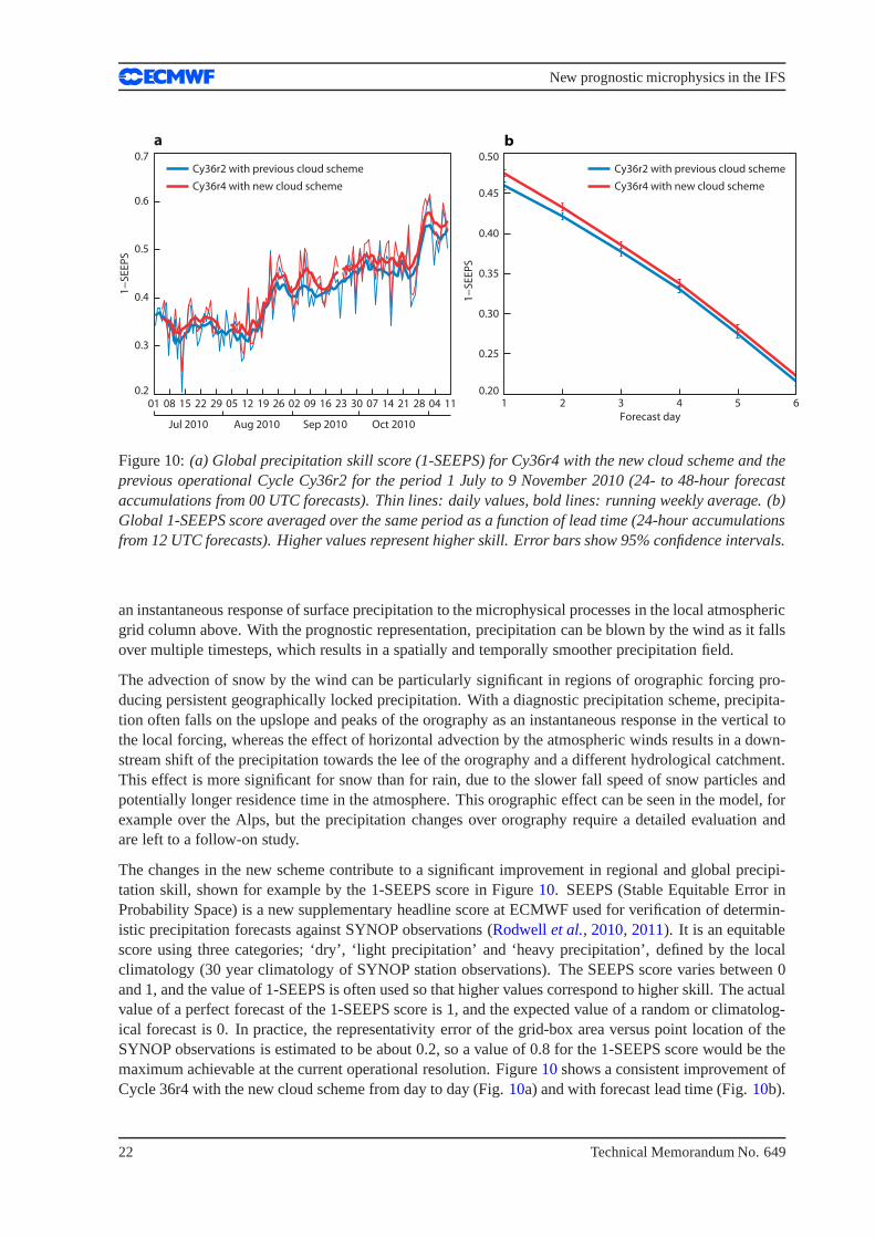
SFigure 10:(a) Global precipitation skill score (1-SEEPS) for Cy36r4 with the new cloud scheme and theprevious operational Cycle Cy36r2 for the period 1 July to 9 November 2010 (24- to 48-hour forecastaccumulations from 00 UTC forecasts). Thin lines: daily values, bold lines: running weekly average. (b)Global 1-SEEPS score averaged over the same period as a function of lead time (24-hour accumulationsfrom 12 UTC forecasts). Higher values represent higher skill. Error bars show 95% confidence intervals.

an instantaneous response of surface precipitation to the microphysical processes in the local atmosphericgrid column above. With the prognostic representation, precipitation can be blown by the wind as it fallsover multiple timesteps, which results in a spatially and temporally smoother precipitation field.

The advection of snow by the wind can be particularly significant in regions of orographic forcing pro-ducing persistent geographically locked precipitation. With a diagnostic precipitation scheme, precipita-tion often falls on the upslope and peaks of the orography as an instantaneous response in the vertical tothe local forcing, whereas the effect of horizontal advection by the atmospheric winds results in a down-stream shift of the precipitation towards the lee of the orography and a different hydrological catchment.This effect is more significant for snow than for rain, due to the slower fall speed of snow particles andpotentially longer residence time in the atmosphere. This orographic effect can be seen in the model, forexample over the Alps, but the precipitation changes over orography require a detailed evaluation andare left to a follow-on study.

The changes in the new scheme contribute to a significant improvement in regional and global precipi-tation skill, shown for example by the 1-SEEPS score in Figure 10. SEEPS (Stable Equitable Error inProbability Space) is a new supplementary headline score atECMWF used for verification of determin-istic precipitation forecasts against SYNOP observations(Rodwellet al., 2010, 2011). It is an equitablescore using three categories; ‘dry’, ‘light precipitation’ and ‘heavy precipitation’, defined by the localclimatology (30 year climatology of SYNOP station observations). The SEEPS score varies between 0and 1, and the value of 1-SEEPS is often used so that higher values correspond to higher skill. The actualvalue of a perfect forecast of the 1-SEEPS score is 1, and the expected value of a random or climatolog-ical forecast is 0. In practice, the representativity errorof the grid-box area versus point location of theSYNOP observations is estimated to be about 0.2, so a value of0.8 for the 1-SEEPS score would be themaximum achievable at the current operational resolution.Figure10shows a consistent improvement ofCycle 36r4 with the new cloud scheme from day to day (Fig.10a) and with forecast lead time (Fig.10b).



4 Concluding Summary

The upgrade to the representation of cloud and precipitation in the IFS has significantly modified thecloud parametrization in terms of the number of prognostic variables, formulation of mixed-phase andprecipitation processes and cloud scheme numerics. The number of prognostic variables has increasedfrom two (cloud fraction, cloud condensate) to five (cloud fraction, cloud liquid water, cloud ice, rainand snow). Liquid and ice cloud condensates are now determined by explicit microphysical processesrather than by a fixed function of temperature, resulting in wider variability of supercooled liquid wateroccurrence. The representations of ice and ice supersaturation in the mixed phase temperature range(0◦C to -23◦C) are improved and snow is now radiatively active. Rain and snow can be advected by thewind and precipitation skill is improved.

Overall, this has been a major change to the representation of moist physics and a significant milestonetowards a more physically based cloud and precipitation parametrization scheme in the IFS model. Theparametrization framework is now more appropriate for a wider range of model resolutions and is closerto the typical single-moment schemes used in higher-resolution limited-area NWP and cloud resolvingmodels (CRMs).

There are many opportunities for further development of thescheme and the focus will shift towards im-proving the formulation of cloud and precipitation microphysical processes to provide a stronger physicalbasis, improved internal consistency and a more direct linkto observable parameters such as particle sizedistributions and particle characteristics. Ongoing evaluation against a wide range of ground based andsatellite observations is a further vital activity for continued parametrization development in the IFS andimproved forecasts of cloud and precipitation in NWP.

Acknowledgements

The authors would like to thank Anton Beljaars, Jean-Jacques Morcrette and colleagues at ECMWFfor many informative discussions, Frank Li and Duane Waliser (JPL) for the processed CloudSat data,Thomas Haiden for the precipitation skill score comparisonand Rob Hine for help with the figures. Weacknowledge the NASA CloudSat project for providing the original data from CloudSat and the ISCCPproject, GPCP project and CERES mission for the observational datasets.



Appendices: Technical notes

A1 Initialising the new rain/snow fields

There is a new logical INIRAINSNOW that needs to be set in the configuration file config.h in sec-tion ”inidata” at IFS Cycle 36r4 onwards which determines whether the model will initialise the newprognostic rain and snow fields from input fields if available, or otherwise initialise to zero.

INIRAINSNOW=false

if there is no existing rain and snow data for initialisation, in which case the prognostic rain and snowfields will be initialised to zero.

INIRAINSNOW=true

if the rain and snow fields are to be initialised from archivedMARS data. The logical is set by prepIFS,defaulting to false if starting from initial fields from model cycles pre-36r4, but defaults to true if startingfrom initial fields from model cycles 36r4 onwards. It takes about 6 hours for the model to spin-upthe snow and rain fields when initialised to zero at the beginning of a forecast run (Figure11 shows anexample).

(a) (b)

Figure 11: Evolution of the global average (a) rain and (b) snow prognostic fields for an exampleT255L91 forecast run (72 hours) when initialised to zero (solid line) compared to initialisation withrain/snow fields from the previous forecast during an analysis cycle (dashed line). The spin-up period isabout 6 hours.



A2 Cloud and precipitation diagnostics

The Grib codes for the ice and liquid water prognostic variables remain unchanged. The new rain andsnow prognostic variables are available on model levels andhave new allocated Grib codes in Grib Table128. There are also two new single level diagnostics available for the vertically integrated rain and snowwater contents (TCRW, TCSW) in Grib Table 228. A list of many of the cloud and precipitation relateddiagnostics is included below.

3D fields (Grib Table 128 unless specified):

Grib code Short name Description Units248 CC Cloud fraction (0-1)246 CLWC Cloud liquid specific water content (kg kg−1)247 CIWC Cloud ice specific water content (kg kg−1)75 CRWC Precipitation rain specific water content (kg kg−1)76 CSWC Precipitation snow specific water content (kg kg−1)130 T Temperature (K)133 Q Specific humidity (kg kg−1)157 RH Relative humidity (only available on pressure levels) (%)

2D fields (Grib Table 128 unless specified):

Grib code Short name Description Units164 TCC Total cloud cover (0-1)186 LCC Low cloud cover (0-1)187 MCC Mid-level cloud cover (0-1)188 HCC High cloud cover (0-1)78 TCLW Total column liquid water (kg m−2)79 TCIW Total column ice water (kg m−2)228089 TCRW Total column rain water (kg m−2)228090 TCSW Total column snow water (kg m−2)142 LSP Accumulated large-scale (stratiform) precipitation (rain+snow) (m)144 SF Accumulated snowfall (stratiform + convective) (m)50 LSPF Accumulated precipitation fraction



References

Adler, R. F., Susskind, J., Huffman, G., Bolvin, D., Nelkin,E., Chang, A., Ferraro, R., Gruber, A.,Xie, P.-P., Janowiak, J., Rudolf, B., Schneider, U., Curtis, S. and Arkin, P. (2003). The version-2Global Precipitation Climatology Project (GPCP) monthly precipitation analysis (1979-present.).J.Hydrometeorol., 4, 1147–1167.

Austin, R. T. (2007). Level 2B radar-only cloud water content (2B-CWC-RO) process description docu-ment.Cloudsat Projects Report, p. 24.

Bouniol, D., Protat, A., Delanoe, J., Pelon, J., Piriou, J.M., Bouyssel, F., Tompkins, A. M., Wilson,D. R., Morille, Y., Haeffelin, M., O’Connor, E. J., Hogan, R.J., Illingworth, A. J., Donovan, D. P. andBaltink, H. K. (2010). Evaluation of operational model cloud representation using routine radar/lidarmeasurements.J. Appl. Meteor. Clim, 49, 1971–1991.

Fu, Q. (1996). An accurate parameterization of the solar radiative properties of cirrus clouds.J. Climate,9, 2058–2082.

Fu, Q., Yang, P. and Sun, W. B. (1998). An accurate parametrization of the infrared radiative propertiesof cirrus clouds of climate models.J. Climate, 11, 2223–2237.

Heymsfield, A. J. and Iaquinta, J. (2000). Cirrus crystal terminal velocities.J. Atmos. Sci., 57, 916–938.

Hogan, R. J., Behera, M. D., O’Connor, E. J. and Illingworth,A. J. (2007). Estimating the global dis-tribution of supercooled liquid water clouds using spaceborne lidar.Geophys. Res. Lett., 32, DOI:10.1029/2003GL018977.

Illingworth, A. J., Hogan, R. J. and coauthors (2007). Cloudnet - Continuous evaluation of cloud profilesin seven operational models using ground-based observations.Bull. Amer. Meteor. Soc., 88, 883–898.

Jakob, C. (2000).The representation of cloud cover in atmospheric general circulation models. Ph.D.thesis, University of Munich, Germany, available from ECMWF, Shinfield Park, Reading RG2 9AX,UK.

Jakob, C. and Klein, S. A. (2000). A parametrization of the effects of cloud and precipitation overlap foruse in general circulation models.Q. J. R. Meteorol. Soc., 126, 2525–2544.

Karcher, B. and Lohmann, U. (2002). A parameterization of cirrus cloud formation: Homogeneousfreezing of supercooled aerosols.J. Geophys. Res., 107, DOI: 10.1029/2001JD000470.

Khvorostyanov, V. and Sassen, K. (1998). Cirrus cloud simulation using explicit microphysics and radia-tion. part ii: Microphysics, vapor and ice mass budgets, andoptical and radiative properties.J. Atmos.Sci., 55, 1822–1845.

Koop, T., Luo, B. P., Tsias, A. and Peter, T. (2000). Water activity as the determinant for homogeneousice nucleation in aqueous solutions.Nature, 406, 611–614.

Lin, Y. L., Farley, R. D. and Orville, H. D. (1983). Bulk parameterization of the snow field in a cloudmodel.J. Climate Appl. Meteorol., 22, 1065–1092.

Lohmann, U. and Karcher, B. (2002). First interactive simulations of cirrus cloud formed byhomogeneous freezing in the ECHAM general circulation model. J. Geophys. Res., 107,10.1029/2001JD000767.



Ma, H.-Y., Kohler, M., Li, J.-L. F., Farrara, J. D., Mechoso,C. R., Forbes, R. M. and Waliser, D. E.(2012). Evaluation of an ice cloud parametrization based ona dynamical-microphysical lifetime con-cept using CloudSat observations and the ERA-Interim reanalysis. J. Geophys. Res., p. Accepted.

Meyers, M. P., DeMott, P. J. and Cotton, W. R. (1992). New primary ice nucleation parameterization inan explicit model.J. Appl. Meteor., 31, 708–721.

Pruppacher, H. R. and Klett, J. D. (1997).The Microphysics of Clouds and Precipitation. Kluwer Aca-demic Publishers, pp. 954.

Ren, C. and Mackenzie, A. R. (2005). Cirrus parametrizationand the role of ice nuclei.Q. J. R. Meteorol.Soc., 131, 1585–1605.

Rodwell, M. J., Haiden, T. and Richardson, D. S. (2011). Developments in precipitation verification.ECMWF Newsletter No., 128, 12–16.

Rodwell, M. J., Richardson, D. S., Hewson, T. D. and Haiden, T. (2010). A new equitable score suitablefor verifying precipitation in numerical weather prediction. Q. J. R. Meteorol. Soc., 136, 1344–1363.

Rossow, W. B. and Schiffer, R. A. (1991). ISCCP cloud data products.Bull. Amer. Meteor. Soc., 72,1–20.

Rossow, W. B., Walker, A., Beuschel, D. and Roiter, M. (1996). International Satellite Cloud Climatol-ogy Project (ISCCP): Description of new cloud datasets. ”WMO/TD-737, World Climate ResearchProgramme (ICSU and WMO), Geneva, Switzerland, 115 pp.”.

Rotstayn, L., Ryan, B. and Katzfey, J. (2000). A scheme for calculation of the liquid fraction in mixed-phase stratiform clouds in large-scale models.Mon. Wea. Rev., 128(4), 1070–1088.

Sun, Z. (2001). Reply to comments by Greg M. McFarquhar on ”Parametrization of effective sizes ofcirrus-cloud particles and its verification against observations”.Q. J. R. Meteorol. Soc., 127, 267–271.

Sun, Z. and Rikus, L. (1999). Parametrization of effective sizes of cirrus-cloud particles and its verifica-tion against observations.Q. J. R. Meteorol. Soc., 125, 3037–3055.

Sundqvist, H. (1978). A parameterization scheme for non-convective condensation including predictionof cloud water content.Q. J. R. Meteorol. Soc., 104, 677–690.

Tiedtke, M. (1993). Representation of clouds in large-scale models.Mon. Wea. Rev., 121, 3040–3061.

Tompkins, A. M., Gierens, K. and Radel, G. (2007). Ice supersaturation in the ECMWF integrated fore-cast system.Q. J. R. Meteorol. Soc., 133, 53–63.

Wacker, U. and Seifert, A. (2001). Evolution of rain water profiles resulting from pure sedimentation:Spectral vs. parameterized description.Atmos. Res., 58, 19–39.

Waliser, D. E., Li, J.-L. F., L’Ecuyer, T. S. and Chen, W.-T. (2011). The impact of precipitatingice and snow on the radiation balance in global climate models. Geophys. Res. Lett., 38, DOI:10.1029/2010GL046478.

Wielicki, B., Barkstrom, B. R., Harrison, E. F., Lee, R. B., Smith, G. L. and Cooper, J. E. (1996). Cloudsand the Earth’s Radiant Energy System (CERES): An Earth observing system experiment.Bull. Amer.Meteor. Soc., 77, 853–868.



Wielicki, B., Priestley, K., Minnis, P., Loeb, N., Kratz, D., Charlock, T., Doelling, D. and Young, D.(2006). CERES radiation budget accuracy overview. In12th Conf. Atmospheric Radiation, Madison,WI, Amer. Meteor. Soc.

Wilson, D. R. and Ballard, S. (1999). A microphysical based precipitation scheme for the UK Meteoro-logical Office Unified Model.Q. J. R. Meteorol. Soc., 125, 1607–1636.


649 - ecmwf · 649 a new prognostic bulk microphysics scheme for the ifs richard m. forbes1, adrian...

Documents