5 exogeneity and causality - nuffield college, oxford · 5 exogeneity and causality ... bines weak...
TRANSCRIPT
5
Exogeneity and Causality
We now consider exogeneity and causality, focusing on their implications for econometric mod-
elling. Causality concerns actual links between variables in the economy, whereas exogeneity
is the property of being ‘determined outside the model under analysis’, so concerns the ana-
lysis of models conditional on putative exogenous variables without loss of relevant information.
Concepts of weak, strong, and super exogeneity relate contemporaneous explanatory variables
to parameters of interest, to sustain valid conditional inference, forecasting, and policy analysis
respectively. Weak exogeneity requires the parameters of conditional and marginal models to
be variation free, and the former to provide the parameters of interest. Strong exogeneity com-
bines weak and Granger causality; while super exogeneity combines weak and the invariance of
conditional parameters to interventions changing marginal parameters. The major goal of this
chapter is investigating sufficient conditions for weak, strong, and super exogeneity of variables
for parameters of interest, in a variety of constant and non-constant models of stationary and coin-
tegrated processes. The chapter also illustrates that weak exogeneity (WE) may help discriminate
between behavioural and contingent models, and that joint stationarity may preclude WE by in-
ducing restrictions across conditional and marginal parameter spaces. Further, non-stationarity
may imply that marginal parameters are functions of the parameters of interest, particularly in
cointegrated processes, although unit roots and either the presence or absence of WE may co-
exist. Conversely, conditional parameters may be functions of the marginal parameters in such a
way that marginal parameters induce restrictions on conditional parameters. In these situations,
conditional and marginal parameters are not variation free, ruling out WE. The notion of WE
also differs from such concepts as strict exogeneity and predeterminedness, which relate explan-
atory variables to disturbances in postulated equations: strict exogeneity and predeterminedness
are often sufficient for consistent estimation, but have nothing to do with the validity of condi-
tional analysis. The exercises show that predeterminedness, strict exogeneity, and the absence
of Granger causality are neither necessary nor sufficient for valid inference. Indeed, predeter-
minedness is an ambiguous concept – because it can be attained by re-writing a model – and in
non-constant processes, may preclude the invariance of parameters to interventions. Zero cross-
equation correlation sometimes guarantees valid conditional inference, but not always, and may
preclude invariance. In practice, testing for Granger causality is carried out by testing for the
significance of past values of the dependent variable in the marginal equation. However, as illus-
trated by these exercises, conclusions drawn from this test are affected by the number of lags, the
131
sample period, choice of variables, and invalid weak exogeneity assumptions. Indeed, empirical
findings of Granger causality, or its absence, need not entail an actual link (or its absence) in the
DGP once non-stationarity is allowed (see Hendry and Mizon, 1997). Exercises 5.1 and 5.2 con-
sider exogeneity conditions in two model types, namely distributed-lag and COMFAC, whereas
§5.3–§5.5 do almost the converse, relating exogeneity to stationarity, model forms, and differen-
cing. These cases are bivariate, so§5.6 examines exogeneity in a trivariate process. Then,§5.7
and§5.8 conclude by discussing exogeneity when the DGP manifests non-constant parameters
and cointegration respectively.
5.1 Exogeneity in a distributed-lag model
Consider the processxt|xt−1 ∼ N2 [Πxt−1,Ω] where:
xt =(
yt
zt
), Π =
(β1β2 β3
β2 0
), Ω =
(ω11 ω12
ω12 ω22
). (5.1)
(1) Derive a conditional model foryt givenzt andxt−1, and establish that its errorvariance is never larger thanω11. Under what conditions iszt weakly exogenousfor (β1, β3)?
(2) Under what conditions iszt strongly exogenous for(β1, β3)?(3) Derive an equation in whichzt is predetermined (i.e., uncorrelated with current
and past errors) even thoughzt is not weakly exogenous for(β1, β3). Are theerrors in that equation: (i) white noise; or (ii) innovations againstxt−1?
(Oxford M.Phil., 1982)
5.1.1 Conditional model
Becausext|xt−1 ∼ N2[Πxt−1,Ω], the conditional distributionyt|zt,xt−1 is also nor-mal with:
E [yt | zt,xt−1] = E [yt | xt−1] +C [yt, zt | xt−1]V [zt | xt−1]
(zt − E [zt | xt−1])
= β1β2yt−1 + β3zt−1 + ω−122 ω12 (zt − β2yt−1)
= δzt + β2 (β1 − δ) yt−1 + β3zt−1 (5.2)
whereδ = ω12ω−122 , and:
V [yt | zt,xt−1] = V [yt | xt−1] − C2 [yt, zt|xt−1]V [zt|xt−1]
= ω11 − ω212
ω22:= ω2. (5.3)
The conditional equation is obtained by writing (5.2) as:
yt = δzt + β2 (β1 − δ) yt−1 + β3zt−1 + νt (5.4)
with νt defined by:νt = yt − E [yt | zt,xt−1] . (5.5)
To show that the variance ofνt cannot be greater than that ofyt|xt−1 notice thatfrom (5.1):
yt = β1β2yt−1 + β3zt−1 + ε1,t (5.6)
whereε1,t is the first element in:
εt =(
ε1,t
ε2,t
)= xt − E [xt | xt−1] (5.7)
so that by comparing the two representations ofyt in (5.4) and (5.6):
νt = ε1,t − δε2,t (5.8)
and asV [νt] = V [ε1,t − δε2,t]:
V [νt] = V [ε1,t] + δ2V [ε2,t] − 2δC [ε1,t, ε2,t] = ω11 − ω212
ω22:= ω2.
Becauseω11 and ω22 are variances, they are non-negative, and asω212 is a squared
quantity, the variance ofνt cannot be larger than the variance ofyt|xt−1, i.e.,ω11 ≥ ω2.This inequality implies that the marginal equation cannot fit better than the conditionalmodel – irrespective of the merits of the latter.
Finally, let us find conditions under whichzt is weakly exogenous for(β1, β3).Weak exogeneity requires two conditions: (i) the parameters of interest must be recov-erable from the parametersφ1 of the conditional distribution alone, and (ii)φ1 and theparametersφ2 of the marginal distributionzt|xt−1 must be variation free. From (5.2)and (5.3):
φ1 =
δ
β2 (β1 − δ)β3
ω2
.
In addition, normality of the joint distribution also implies that:
zt | xt−1 ∼ N [β2yt−1, ω22] (5.9)
and so:
φ2 =(
β2
ω22
).
Hence, a sufficient condition forzt to be weakly exogenous for(β1, β3) is thatβ1 = δ,because thenφ1 = (β1 : β3 : ω2)′ implying that the parameters of interest(β1, β3) canbe obtained from the parameters of the conditional distribution alone; and, in addition,
φ1 andφ2 are variation free because, apart from the conditions forΩ to be positivedefinite, knowledge of the values thatφ2 can take does not provide information on theparameter space ofφ1, at least if joint stationarity is not enforced. Thus, for weakexogeneity, the error covarianceω12 = β1ω22 must involve the same parameter (β1)as the conditional model. Such an outcome will arise when the joint is derived fromthe conditional plus the marginal, and the latter pair characterize the behaviour of therelevant economic agents. Indeed, the resulting equation is the distributed lag:
yt = β1zt + β3zt−1 + νt.
By writing the system in (5.1) as:(∆yt
∆zt
)=(
β1β2 − 1 β3
β2 −1
)(yt−1
zt−1
)+(
ε1,t
ε2,t
)joint stationarity requires:
det(
β1β2 − 1 β3
β2 −1
)6= 0
which is satisfied ifβ2(β1 + β3) 6= 1. Hence, joint stationarity places restrictionsacross conditional and marginal parameters, ruling out the property of variation-freeparameters and hence precluding weak exogeneity ofzt for (β1, β3). We exclude thiscase below.
5.1.2 Strong exogeneity
Strong exogeneity requires weak exogeneity plus the absence of Granger causality. Wehave already seen that weak exogeneity is satisfied ifβ1 = δ. By definition, Grangernon-causality is satisfied if:
Dz (zt | Xt−1; ·) = Dz (zt | Zt−1; ·) ,
i.e., if the distribution ofzt conditional on the past is not a function of pastys. From(5.9),β2 = 0 suffices for Granger non-causality, because then:
zt | xt−1 ∼ N [0, ω22] .
Hence, underβ1 = δ and β2 = 0, zt is strongly exogenous for(β1, β3). Noticethat strong exogeneity here allows stationarity to be determined from the equationsseparately.
5.1.3 Predeterminedness
We will show thatzt is predetermined in (5.4), irrespective of its weak exogeneitystatus forβ1. To do so, we need to check whetherE[zt−iνt] = 0, for all i ≥ 0. Because
stationarity implies thatE[zt−iνt] = E[ztνt+i], we will derive the latter expectationinstead. From (5.1), we can writezt in terms of pastεs using:
xt =[I2 −
(β1β2 β3
β2 0
)L
]−1
εt
=(1 − β1β2L − β2β3L
2)−1
(1 β3L
β2L 1 − β1β2L
)εt (5.10)
and forξ1 6= ξ2,(1 − β1β2L − β2β3L
2)−1
can be factorized as:(1 − β1β2L − β2β3L
2)−1
= [(1 − ξ1L) (1 − ξ2L)]−1
=1
(ξ1 − ξ2)L
(1
1 − ξ1L− 1
1 − ξ2L
).
Hence, from (5.10),zt can be written as (L−1ε2,t = ε2,t+1):
zt =1
ξ1 − ξ2
(1
1 − ξ1L− 1
1 − ξ2L
)(β2ε1,t + [1 − β1β2L] ε2,t+1)
=1
ξ1 − ξ2
∞∑j=0
(ξj1 − ξj
2
)[β2ε1,t−j + ε2,t−j+1 − β1β2ε2,t−j]
. (5.11)
Consequently, from (5.8) and (5.11), when theεs are serially uncorrelated:
E [ztνt+i] =1
ξ1 − ξ2
∞∑j=0
(ξj1 − ξj
2
)×E [(β2ε1,t−j + ε2,t−j+1 − β1β2ε2,t−j) (ε1,t+i − δε2,t+i)] (5.12)
which is zero for alli ≥ 0, because fori > 0 all expectations are zero, and fori = 0expectations are different from zero only forj = 0 in which caseξj
1 − ξj2 = 0. So,zt is
predetermined in (5.4).Equation (5.4) has a number of desirable properties: its disturbances are white noise
and innovations against the information contained in(zt,xt−1) when theεs are seriallyuncorrelated. To see thatνt is white noise, we notice from (5.8) thatE[νt] = 0 and havefoundV[νt] = ω2, and so both moments are constant over time. Thus, we just need toshow that theνt are serially uncorrelated. To do so, consider:
E [νtνt−τ ] = E [(ε1,t − δε2,t) (ε1,t−τ − δε2,t−τ )]
= E [ε1,tε1,t−τ ] − δE [ε1,tε2,t−τ ] − δE [ε2,tε1,t−τ ] + δ2E [ε2,tε2,t−τ ] ,
which is zero for allτ > 0, soνt is serially uncorrelated.
Finally, νt is an innovation against(zt,xt−1) because taking expectations in (5.5)implies that:
E [νt | zt,xt−1] = E [yt | zt,xt−1] − E [yt | zt,xt−1] = 0.
Summarizing,zt is predetermined in the conditional equation in (5.4), and the dis-turbances in that equation are white noise and innovations with respect to(zt,xt−1).However,zt is not weakly exogenous for the parameters in that equation whenβ1 6= δ,proving that predeterminedness is insufficient for valid conditional inference. This lackcan have serious consequences: for example, ifβ2 were to change, then (5.4) wouldalso change unlesszt was weakly exogenous forβ1.
5.2 Exogeneity in aCOMFAC model
Consider the system:yt = βzt + ut
ut = ρut−1 + ε1,t
zt = αyt−1 + ε2,t
(5.13)
where: (ε1,t
ε2,t
)∼ IN2
[(00
),
(σ11 σ12
σ12 σ22
)], (5.14)
with |ρ| < 1.
(1) Iszt predetermined in (5.13)?(2) Derive a form of equation in whichzt is predetermined.(3) Iszt weakly exogenous forβ whenρ 6= 0? (Hint: can you deriveβ uniquely and
unrestrictedly fromE [yt|zt, yt−1, zt−1]?).(4) Under what conditions iszt strongly exogenous forβ?(5) Under what conditions iszt strictly exogenous in (5.13)?(6) If zt is predetermined in (5.13) whenσ12 6= 0, show thatβ = E [ytzt] /E
[z2
t
].
What is the economic rationale for the resulting model? Hence (or otherwise)show thatE [ztut−1] 6= 0, so that ‘taking account’ of the autocorrelation in (5.13)must now yield inconsistent estimates ofβ. (Hint: first showE [ztε1,t] 6= 0.)
(7) If ρ = 0, under what conditions iszt weakly exogenous forβ? Comment on thistype of model, and its economic interpretation (See Engle, Hendry and Richard,1983).
(8) Test for Granger causality betweenCONSandINC; and betweenOUTPUTandINFLAT. What do you conclude in each case? Does the length of lag used matter?Does the sample period selected matter? Would the unknown existence of otherGranger-causality links alter the results in a substantive way (e.g. reverse yourconclusions)? Did you test for any other cross connections? In both directions?
(9) Repeat§5.2.8 for the UKM1 data set, usingM/Pt andYt; Rt and∆log Pt.
(Oxford M.Phil., 1985, extended)
5.2.1 Predeterminedness
zt is predetermined in (5.13a) ifE[zt−iut] = 0 for all i ≥ 0. Assuming stationarity,E[zt−iut] = E[ztut+i], so we will check whetherE[ztut+i] = 0. To do so, notice thatby substituting (5.13a) into (5.13c),zt can be written as:
zt = αβzt−1 + αut−1 + ε2,t (5.15)
so that:
E [ztut] = E [(αβzt−1 + αut−1 + ε2,t) (ρut−1 + ε1,t)]
= αβρE [zt−1ut−1] + αβE [zt−1ε1,t] + αρE[u2
t−1
]+ αE [ut−1ε1,t]
+ρE [ε2,tut−1] + E [ε1,tε2,t] ,
and stationarity implies that:
E [ztut] = αβρE [ztut] + αβE [zt−1ε1,t] + αρE[u2
t
]+ αE [ut−1ε1,t] (5.16)
+ρE [ε2,tut−1] + E [ε1,tε2,t] .
Serial independence of theεt, as assumed in (5.14), allows us to obtain the followingresults for each term in (5.16) separately. First, however, note that (5.13) can be writtenas:
xt :=(
yt
zt
)=(
βα + ρ −ρβ
α 0
)(yt−1
zt−1
)+(
1 β
0 1
)(ε1,t
ε2,t
). (5.17)
The eigenroots of this dynamic system are given by solving forξ from:
det(
ξ − (βα + ρ) ρβ
−α ξ
)= ξ2 − ξ (βα + ρ) + αρβ = 0,
yielding the rootsξ1 = αβ andξ2 = ρ , so stationarity requires that|βα| < 1.To derive the second term in (5.16), notice that (5.13b) can be written as:
ut = (1 − ρL)−1 ε1,t =∞∑
j=0
ρjε1,t−j
so that, forαβ 6= ρ, (5.15) is:
zt = (1 − αβL)−1 (αut−1 + ε2,t)
= (1 − αβL)−1[α (1 − ρL)−1 ε1,t−1 + ε2,t
]=
α
(αβ − ρ)L
(1
1 − αβL− 1
1 − ρL
)ε1,t−1 + (1 − αβL)−1
ε2,t
=α
αβ − ρ
∞∑j=0
[(αβ)j − ρj
]ε1,t−j +
∞∑j=0
(αβ)jε2,t−j . (5.18)
Thus, the second term forE[zt−1ε1,t] in (5.16) is:
α
αβ − ρ
∞∑j=0
[(αβ)j − ρj
]E [ε1,tε1,t−j−1] +
∞∑j=0
(αβ)j E [ε1,tε2,t−j−1] = 0.
The remaining terms are:
E[u2
t
]= E
∞∑j=0
ρjε1,t−j
∞∑j=0
ρjε1,t−j
= E
∞∑j,k=0
ρj+kε1,t−jε1,t−k
=
∞∑j=0
ρ2jE[ε21,t
]=
σ11
1 − ρ2 ,
E [ut−1ε1,t] =∞∑
j=0
ρjE [ε1,t−j−1ε1,t] = 0,
and:
E [ε2,tut−1] =∞∑
j=0
ρjE [ε1,t−j−1ε2,t] = 0.
Also, E[ε1,tε2,t] = σ12, so that collecting terms and noting|αβρ| < 1:
E [ztut] =1
1 − αβρ
(αρσ11
1 − ρ2+ σ12
)6= 0 (5.19)
in general, sozt is not predetermined in (5.13a) whenαρσ11 6= −σ12(1 − ρ2).In addition, we can show thatE[ztut+i] 6= 0, for i > 0. To do so, substitute back-
wards in:ut+i = ρut+i−1 + ε1,t+i,
to get:
ut+i = ρ (ρut+i−2 + ε1,t+i−1) + ε1,t+i
= ρiut +i−1∑j=0
ρjε1,t+i−j,
and so:
E [ztut+i] = E
zt
ρiut +i−1∑j=0
ρjε1,t+i−j
= ρiE [ztut] +
i−1∑j=0
ρjE [ztε1,t+i−j ] .
But from (5.18),E[ztε1,t+i−j ] = 0 for all i > j and so (5.19) implies:
E [ztut+i] = ρiE [ztut] = ρi (1 − αβρ)−1
(αρσ11
1 − ρ2+ σ12
)6= 0. (5.20)
Hence,αρσ11 = −σ12(1 − ρ2) is sufficient for predeterminedness ofzt in (5.13).
5.2.2 Derived predeterminedness
However, predeterminedness in (5.13) can be attained by rewriting equation (5.13a). Tosee that, notice that from (5.14)(ε1,t : ε2,t)
′ is normally distributed, and hence so is thefollowing linear combination:(
1 β
0 1
)(ε1,t
ε2,t
)∼ N2
[(00
),
(1 β
0 1
)(σ11 σ12
σ21 σ22
)(1 0β 1
)](5.21)
which we denote byN2 [0,Ω], with:
Ω =(
σ11 + 2βσ12 + β2σ22 σ12 + βσ22
σ12 + βσ22 σ22
).
From (5.17)+(5.21), the conditional distribution is:
xt | xt−1 ∼ N2
[(βα + ρ −ρβ
α 0
)(yt−1
zt−1
),Ω]
(5.22)
and soyt|zt,xt−1 is also normal with:
E [yt | zt,xt−1] = E [yt | xt−1] +C [yt, zt | xt−1]V [zt | xt−1]
(zt − E [zt | xt−1])
= (βα + ρ) yt−1 − ρβzt−1 +σ12 + βσ22
σ22(zt − αyt−1)
= (β + δ) zt + (ρ − δα) yt−1 − ρβzt−1 (5.23)
whereδ = σ12σ−122 , and:
V [yt | zt,xt−1] = V [yt | xt−1] − C2 [yt, zt | xt−1]V [zt | xt−1]
= σ11 + 2βσ12 + β2σ22 − (σ12 + βσ22)2
σ22
= σ11 − σ212
σ22:= σ2. (5.24)
We now show thatzt is predetermined in the following conditional equation derivedfrom (5.23):
yt = (β + δ) zt + (ρ − δα) yt−1 − ρβzt−1 + νt (5.25)
where:νt = yt − E [yt | zt,xt−1] . (5.26)
To do so, notice that (5.13a,b) imply:
yt = βzt + ρyt−1 − ρβzt−1 + ε1,t (5.27)
so that from (5.25) and (5.27):
νt = ε1,t − δε2,t. (5.28)
Therefore, from (5.18):
E [ztνt+i] =α
αβ − ρ
∞∑j=0
[(αβ)j − ρj
]E [ε1,t−j (ε1,t+i − δε2,t+i)]
+∞∑
j=0
(αβ)jE [ε2,t−j (ε1,t+i − δε2,t+i)]
= 0,
for all i ≥ 0, because all expectations are zero in the second term, and expectations inthe first term differ from zero only fori = j = 0 in which case(αβ)j − ρj = 0. Thus,althoughzt is only predetermined in (5.13a) whenαρσ11 = −(1 − ρ2)σ12, and is notpredetermined in (5.27),zt is predetermined in the ‘look alike’ equation (5.25) showingthat predeterminedness is an ambiguous concept.
Equation (5.25) has some desirable properties. We can show thatνt is white noisebecause from (5.28),E[νt] = 0, and:
V[νt] = V[ε1,t − δε2,t] = σ11 − σ212σ
−122 := σ2,
so both moments are constant over time, and:
E [νtνt−τ ] = E [(ε1,t − δε2,t) (ε1,t−τ − δε2,t−τ )] = 0,
so thatνt is serially uncorrelated (in fact, it is serially independent due to normal-ity). In addition, νt is an innovation against(zt,xt−1) because (5.26) implies thatE[νt|zt,xt−1] = 0.
5.2.3 Weak exogeneity under autocorrelation
From (5.23) and (5.24) the parameters of the conditional distribution are:
φ1 =
β + δ
ρ − δα
−ρβ
σ2
.
In addition, (5.22) implies that the marginal distribution is:
zt | xt−1 ∼ N [αyt−1, σ22]
and so its parameters are:
φ2 =(
α
σ22
).
Hence,zt could be weakly exogenous forβ even ifρ 6= 0. In fact,σ12 = δ = 0 is asufficient condition because then:
φ1 =
β
ρ
−ρβ
σ11
,
so β is recoverable fromφ1 alone, and knowledge about the parameter space ofφ2
does not provide information on the valuesφ1 can take, implying thatφ1 andφ2 arevariation free as long as joint stationarity is not required. However, because the thirdelement inφ1 implies a restriction between the first and second elements, straightOLS
is not efficient as it ignores restriction. If joint stationarity is imposed,φ1 andφ2 areno longer variation free because stationarity imposes restrictions acrossφ1 andφ2. Asshown above, for stationarity, the roots must be inside the unit circle, i.e.,|βα|, |ρ| < 1.Hence,|βα| < 1 imposes a restriction betweenα andβ, and so onto the parameterspaces ofφ1 andφ2. Note that|β| < 1 and|α| < 1 would be sufficient for stationarity(if they were true), and would still allow weak exogeneity.
An alternative sufficient condition for weak exogeneity ofzt for β, and one whichis independent of stationarity, isα = 0, since:
φ1 =
β + δ
ρ
−ρβ
σ2
,
and henceβ can be obtained as the ratio of the third to the second elements inφ1, andφ1 andφ2 are variation free even if stationarity is required.OLS on the conditionalmodel identifies the parameters
(ρ, −βρ, β + δ, σ2
), which are now in a one-to-one
relationship with the underlying parameters of interest (which still operate a cut withrespect to the remaining nuisance parameterσ22).
5.2.4 Strong exogeneity
For strong exogeneity, we require weak exogeneity and Granger non-causality. Weakexogeneity is satisfied ifα = 0, which also implies Granger non-causality because then:
zt | xt−1 ∼ N [0, σ22] ,
and hence this marginal distribution is independent of pastys. Thus,α = 0 implies thatzt is strongly exogenous forβ. Conversely,δ = 0 is sufficient for weak exogeneity forβ, but not strong when|β| < 1 and|α| < 1 with α 6= 0.
5.2.5 Strict exogeneity
Strict exogeneity ofzt in equation (5.13a) requiresE[ztus] = 0 for all t, s. Also,(5.19) and (5.20) imply thatE[ztut+i] = 0 if αρσ11 = −(1 − ρ2)σ12, for all i ≥ 0.Consider nowE[ztut−i]. To derive this quantity, writezt in terms of laggedzs andεs.Substituting backwards in (5.15):
zt = αiβizt−i +i∑
j=1
αjβj−1ut−j +i−1∑j=1
αjβjε2,t−j,
and henceE [ztut−i] equals:
αiβiE [zt−iut−i] +i∑
j=1
αjβj−1E [ut−jut−i] +i−1∑j=1
αjβjE [ε2,t−jut−i]
=αiβi
1 − αβρ
(αρσ11
1 − ρ2+ σ12
)+
i∑j=1
αjβj−1 ρi−jσ11
1 − ρ2
+i−1∑j=1
αjβjE [ε2,t−jut−i] .
But, becausej < i in the third term and theεs are serially independent:
E [ε2,t−jut−i] =∞∑
k=0
ρkE [ε2,t−jε1,t−k−i] = 0,
so that:
E [ztut−i] =αiβi
1 − αβρ
(αρσ11
1 − ρ2+ σ12
)+
α(ρi − αiβi
)σ11
(1 − ρ2)(ρ − αβ)(5.29)
and henceα = 0 is a sufficient condition forE[ztut−i] = 0. Thus, the followingtwo conditions are sufficient for strict exogeneity in (5.13a):α = 0 andαρσ11 =−(1 − ρ2)σ12, which enforceσ12 = 0. We have already shown thatzt is weaklyexogenous forβ if α = 0 even ifσ12 6= 0, which proves that strict exogeneity is notnecessary for weak exogeneity.
5.2.6 Economic rationale
Sincezt is predetermined in (5.13a) ifE[ztut+i] = 0 for all i ≥ 0, then (5.19) and(5.20) imply thatzt is predetermined ifαρσ11 = −(1 − ρ2)σ12. So, we will show
that if zt is predetermined in (5.13a), thenβ = E[ytzt]/E[z2t ]. To do that notice that
equation (5.13a) implies:
E [ytzt] = βE[z2
t
]+ E [ztut] ,
so that, ifzt is predetermined in (5.13a), i.e., ifE[ztut] = 0, then:
β =E [ytzt]E [z2
t ].
Under predeterminedness, equation (5.13a) looks as a legitimate static model becauseE[ut|zt] = 0. However, there is a loss of information from estimating (5.13a) alonebecauseut is not an innovation againstxt−1, i.e., E[ut|yt−1, zt−1] 6= 0. To see that,notice that from (5.13a):
E [ut | yt−1, zt−1] = E [yt | yt−1, zt−1] − βE [zt | yt−1, zt−1] ,
so that from (5.17):
E [ut | yt−1, zt−1] = (αβ + ρ)yt−1 − ρβzt−1 − αβyt−1 = ρut−1 6= 0.
Nevertheless, many economic theories are represented by static models.Rather than looking at (5.13a), consider (5.25) and notice that it is a COMFAC
representation fory. COMFAC models rarely have a useful economic interpreta-tion (see§7.1.2 (ii) below). In addition, in this particular example, (5.26) implies thatE[νt|zt] = 0 and so thatE[(ε1,t − δε2,t)zt] = 0 which in turn implies that:
E [ε1,tzt] =σ12
σ22E [ε2,tzt] .
But (5.18) implies that:
E [ztε2,t] =α
αβ − ρ
∞∑j=0
[(αβ)j − ρj
]E [ε2,tε1,t−j ] +
∞∑j=0
(αβ)jE [ε2,tε2,t−j]
= σ22,
and soE[ε1,tzt] = σ12. Hence, if predeterminedness is attained by:
σ12 = −αρσ11
1 − ρ2,
thenσ12 6= 0 if α, ρ, andσ11 are all different from zero, and henceOLS cannot beconsistent in (5.25). Thus,OLS is consistent in the equation with an autoregressiveerror, but ceases to be consistent when the autocorrelation is removed.
One possible economic rationale is the relation between spot and forward prices:when the latter lead by several periods, there must be serial correlation from the ‘miss-ing’ information. The desire to model this serial dependence in the error process, rather
than using say the generalized method of moments leaving residual autocorrelation,would induce inconsistent estimates. Indeed, theOLS estimators ofβ in (5.13a), andof ρ in (5.13b) using theOLS residuals, are consistent. But, if we then ‘correct’ forautocorrelation in the Cochrane–Orcutt manner byOLS on:
(yt − ρyt−1) = β (zt − ρzt−1) + ε1,t,
the estimate ofβ is inconsistent sinceE[ztε1,t] 6= 0.
5.2.7 Weak exogeneity with no autocorrelation
The conditionρ = 0 implies that the parameters of the conditional model are:
φ1 =
β + δ
−δα
σ2
.
Thus, as in§5.2.3,σ12 = 0 suffices for weak exogeneity ofzt for β because thenφ1 = (β, σ2)′, so thatβ can be obtained fromφ1 alone, andφ1 andφ2 are variationfree when joint stationarity is not required. If so,σ12 = α = 0 is a sufficient conditionfor weak exogeneity. Also,ρ = 0 implies that (5.13) is:
yt = βzt + ε1,t
zt = αyt−1 + ε2,t,
so that if variables are in logarithms, this model can be interpreted as a cobweb system inwhichyt andzt are logarithms of prices and quantities, respectively. The first equationis derived from a demand equation in which prices clear the market if the quantity iszt.Thenβ−1 is the price elasticity of demand. The second equation is a supply equation,entailing that decisions on quantities are based on the previous period’s prices, andα
is the price elasticity of supply (see Ericsson, 1992, p.257)). The first equation is astatic model, so that dynamics are believed to be irrelevant. In addition,zt is weaklyexogenous forβ whenσ12 = 0 and|αβ| < 1 is not imposed.
5.2.8 Granger causality on artificial data
Often, in practice, Granger causality is tested by checking for the significance of lagsof the potential causal variables in simple linear dynamic equations. Let us proceed inthis way in this example to learn about the pitfalls of such a procedure. For instance, wewill examine whether the number of lags and the sample period affect the conclusionsderived from such tests. Hence, we estimate models with a constant and up to thehighest significant lag, for the whole sample period, 1953(3)–1992(3), and the sub-sample 1953(3)–1973(4). The results are shown in Table 5.1 forCONSandINC, andfor OUTPUTandINFLAT, in both directions.
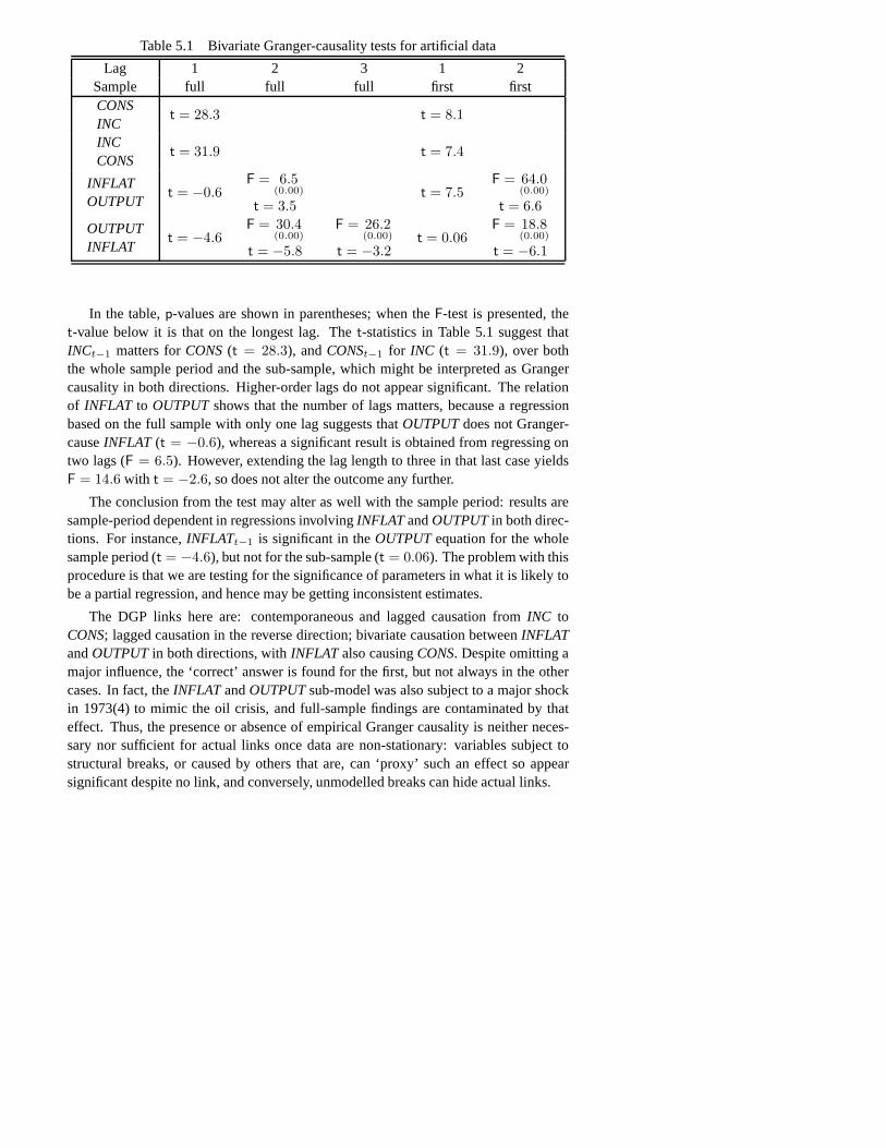
Table 5.1 Bivariate Granger-causality tests for artificial data
Lag 1 2 3 1 2Sample full full full first firstCONSINC
t = 28.3 t = 8.1
INCCONS
t = 31.9 t = 7.4
INFLATOUTPUT
t = −0.6F = 6.5
(0.00)
t = 3.5t = 7.5
F = 64.0(0.00)
t = 6.6
OUTPUTINFLAT
t = −4.6F = 30.4
(0.00)
t = −5.8
F = 26.2(0.00)
t = −3.2t = 0.06
F = 18.8(0.00)
t = −6.1
In the table,p-values are shown in parentheses; when theF-test is presented, thet-value below it is that on the longest lag. Thet-statistics in Table 5.1 suggest thatINCt−1 matters forCONS(t = 28.3), andCONSt−1 for INC (t = 31.9), over boththe whole sample period and the sub-sample, which might be interpreted as Grangercausality in both directions. Higher-order lags do not appear significant. The relationof INFLAT to OUTPUTshows that the number of lags matters, because a regressionbased on the full sample with only one lag suggests thatOUTPUTdoes not Granger-causeINFLAT (t = −0.6), whereas a significant result is obtained from regressing ontwo lags (F = 6.5). However, extending the lag length to three in that last case yieldsF = 14.6 with t = −2.6, so does not alter the outcome any further.
The conclusion from the test may alter as well with the sample period: results aresample-period dependent in regressions involvingINFLATandOUTPUTin both direc-tions. For instance,INFLATt−1 is significant in theOUTPUTequation for the wholesample period (t = −4.6), but not for the sub-sample (t = 0.06). The problem with thisprocedure is that we are testing for the significance of parameters in what it is likely tobe a partial regression, and hence may be getting inconsistent estimates.
The DGP links here are: contemporaneous and lagged causation fromINC toCONS; lagged causation in the reverse direction; bivariate causation betweenINFLATandOUTPUTin both directions, withINFLAT also causingCONS. Despite omitting amajor influence, the ‘correct’ answer is found for the first, but not always in the othercases. In fact, theINFLAT andOUTPUTsub-model was also subject to a major shockin 1973(4) to mimic the oil crisis, and full-sample findings are contaminated by thateffect. Thus, the presence or absence of empirical Granger causality is neither neces-sary nor sufficient for actual links once data are non-stationary: variables subject tostructural breaks, or caused by others that are, can ‘proxy’ such an effect so appearsignificant despite no link, and conversely, unmodelled breaks can hide actual links.
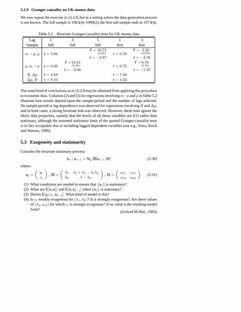
5.2.9 Granger causality on UK-money data
We now repeat the exercise in§5.2.8, but in a setting where the data-generation processis not known. The full sample is 1963(4)–1989(2); the first sub-sample ends in 1973(4).
Table 5.2 Bivariate Granger-causality tests for UK money data
Lag 1 3 5 1 3Sample full full full first first
m − p, y t = 5.66F = 16.73
(0.00)
t = −2.67t = 0.16
F = 3.26(0.036)
t = −2.56
y, m − p t = 6.06F =19.24
(0.00)
t = −2.06t = 0.75
F =0.70(0.56)
t = −1.25R, ∆p t = 8.68 t = 7.04∆p, R t = 8.10 t = 4.33
The same kind of conclusions as in§5.2.8 may be obtained from applying this procedureto economic data. Columns (2) and (5) for regressions involvingm−p andy in Table 5.2illustrate how results depend upon the sample period and the number of lags selected.No sample period or lag dependence was observed for regressions involvingR and∆p,and in both cases, a strong bivariate link was observed. However, these tests ignore thelikely data properties, namely that the levels of all these variables areI(1) rather thanstationary, although the assumed stationary basis of the quoted Granger-causality testsis in fact acceptable due to including lagged dependent variables (see e.g., Sims, Stockand Watson, 1990).
5.3 Exogeneity and stationarity
Consider the bivariate stationary process:
xt | xt−1 ∼ N2 [Πxt−1,Ω] (5.30)
where:
xt =(
yt
zt
), Π =
(λ1 λ3 + λ2 − λ1λ2
λ3 1 − λ3
), Ω =
(ω11 ω12
ω12 ω22
). (5.31)
(1) What conditions are needed to ensure thatxt is stationary?(2) What areE[xtx′
t] andE[xtx′t−1] whenxt is stationary?
(3) DeriveE[yt|zt,xt−1]. What kind of model is this?(4) Is zt weakly exogenous for(λ1, λ2)? Is it strongly exogenous? Are there values
of (λ3, ω12) for whichzt is strongly exogenous? If so, what is the resulting modelform?
(Oxford M.Phil., 1983)
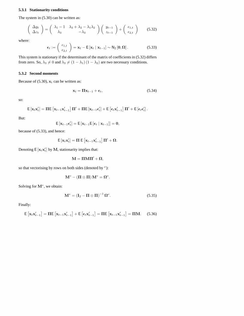
5.3.1 Stationarity conditions
The system in (5.30) can be written as:(∆yt
∆zt
)=(
λ1 − 1 λ3 + λ2 − λ1λ2
λ3 −λ3
)(yt−1
zt−1
)+(
ε1,t
ε2,t
)(5.32)
where:
εt :=(
ε1,t
ε2,t
)= xt − E [xt | xt−1] ∼ N2 [0,Ω] . (5.33)
This system is stationary if the determinant of the matrix of coefficients in (5.32) differsfrom zero. So,λ3 6= 0 andλ3 6= (1 − λ1) (1 − λ2) are two necessary conditions.
5.3.2 Second moments
Because of (5.30),xt can be written as:
xt = Πxt−1 + εt, (5.34)
so:
E [xtx′t] = ΠE
[xt−1x′
t−1
]Π′ + ΠE [xt−1ε
′t] + E
[εtx′
t−1
]Π′ + E [εtε
′t] .
But:E [xt−1ε
′t] = E [xt−1E [εt | xt−1]] = 0,
because of (5.33), and hence:
E [xtx′t] = Π E
[xt−1x′
t−1
]Π′ + Ω.
DenotingE [xtx′t] by M, stationarity implies that:
M = ΠMΠ′ + Ω,
so that vectorising by rows on both sides (denoted byν):
Mv − (Π⊗ Π)Mv = Ωv.
Solving forMv, we obtain:
Mv = (I2 − Π⊗ Π)−1 Ωv. (5.35)
Finally:
E[xtx′
t−1
]= ΠE
[xt−1x′
t−1
]+ E
[εtx′
t−1
]= ΠE
[xt−1x′
t−1
]= ΠM. (5.36)
5.3.3 Conditional equation
BecauseDx(xt|xt−1, ·) is normal, the conditionalDy|z(yt|zt,xt−1, ·) is also normalwith meanE[yt|zt,xt−1] given by:
E [yt | xt−1] − C [yt, zt|xt−1]V [zt|,xt−1]
(zt − E [zt | xt−1])
= λ1yt−1 + [λ3 + λ2 (1 − λ1)] zt−1 +ω12
ω22[zt − λ3yt−1 − (1 − λ3) zt−1]
= γzt + [λ1 − γλ3] yt−1 + [λ3 + λ2 (1 − λ1) − (1 − λ3) γ] zt−1 (5.37)
whereγ = ω12ω−122 , which can also be written as the following conditional equation:
yt = γzt + [λ1 − γλ3] yt−1 + [λ3 + λ2 (1 − λ1) − (1 − λ3) γ] zt−1 + ηt (5.38)
with:
ηt = yt − E [yt | zt,xt−1] .
Equation (5.38) turns out to beAD(1,1).
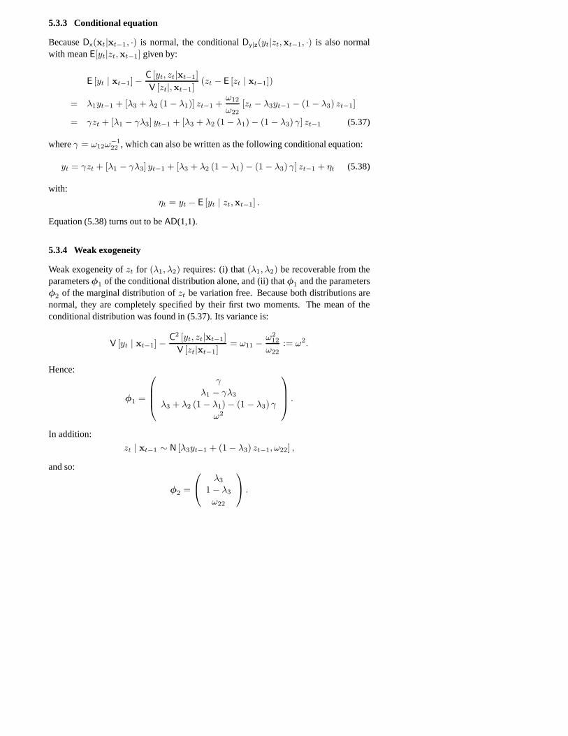
5.3.4 Weak exogeneity
Weak exogeneity ofzt for (λ1, λ2) requires: (i) that(λ1, λ2) be recoverable from theparametersφ1 of the conditional distribution alone, and (ii) thatφ1 and the parametersφ2 of the marginal distribution ofzt be variation free. Because both distributions arenormal, they are completely specified by their first two moments. The mean of theconditional distribution was found in (5.37). Its variance is:
V [yt | xt−1] − C2 [yt, zt|xt−1]V [zt|xt−1]
= ω11 − ω212
ω22:= ω2.
Hence:
φ1 =
γ
λ1 − γλ3
λ3 + λ2 (1 − λ1) − (1 − λ3) γ
ω2
.
In addition:
zt | xt−1 ∼ N [λ3yt−1 + (1 − λ3) zt−1, ω22] ,
and so:
φ2 =
λ3
1 − λ3
ω22
.
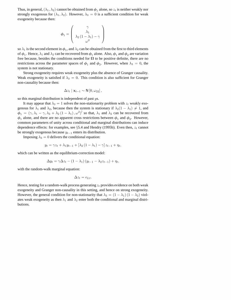
Thus, in general,(λ1, λ2) cannot be obtained fromφ1 alone, sozt is neither weakly norstrongly exogenous for(λ1, λ2). However,λ3 = 0 is a sufficient condition for weakexogeneity because then:
φ1 =
γ
λ1
λ2 (1 − λ1) − γ
ω2
soλ1 is the second element inφ1, andλ2 can be obtained from the first to third elementsofφ1. Hence,λ1 andλ2 can be recovered fromφ1 alone. Also,φ1 andφ2 are variationfree because, besides the conditions needed forΩ to be positive definite, there are norestrictions across the parameter spaces ofφ1 andφ2. However, whenλ3 = 0, thesystem is not stationary.
Strong exogeneity requires weak exogeneity plus the absence of Granger causality.Weak exogeneity is satisfied ifλ3 = 0. This condition is also sufficient for Grangernon-causality because then:
∆zt | xt−1 ∼ N [0, ω22] ,
so this marginal distribution is independent of pastys.It may appear thatλ3 = 1 solves the non-stationarity problem withzt weakly exo-
genous forλ1 andλ2, because then the system is stationary ifλ2(1 − λ1) 6= 1, andφ1 = (γ, λ1 − γ, λ3 + λ2 (1 − λ1) , ω2)′ so that,λ1 andλ2 can be recovered fromφ1 alone, and there are no apparent cross restrictions betweenφ1 andφ2. However,common parameters of unity across conditional and marginal distributions can inducedependence effects: for examples, see§5.4 and Hendry (1995b). Even then,zt cannotbe strongly exogenous becauseyt−1 enters its distribution.
Imposingλ3 = 0 delivers the conditional equation:
yt = γzt + λ1yt−1 + [λ2 (1 − λ1) − γ] zt−1 + ηt,
which can be written as the equilibrium-correction model:
∆yt = γ∆zt − (1 − λ1) (yt−1 − λ2zt−1) + ηt,
with the random-walk marginal equation:
∆zt = ε2,t.
Hence, testing for a random-walk process generatingzt provides evidence on both weakexogeneity and Granger non-causality in this setting, and hence on strong exogeneity.However, the general condition for non-stationarity thatλ3 = (1 − λ1) (1 − λ2) viol-ates weak exogeneity as thenλ1 andλ2 enter both the conditional and marginal distri-butions.
Finally, ω12 = 0 = γ yields:
φ1 =
λ1
λ3 + λ2 (1 − λ1)ω11
,
so thatλ1 andλ2 cannot be obtained fromφ1 alone, and hencezt is not weakly exo-genous for those parameters. This is a case in which zero cross-equation correlationdoes not suffice for weak exogeneity.
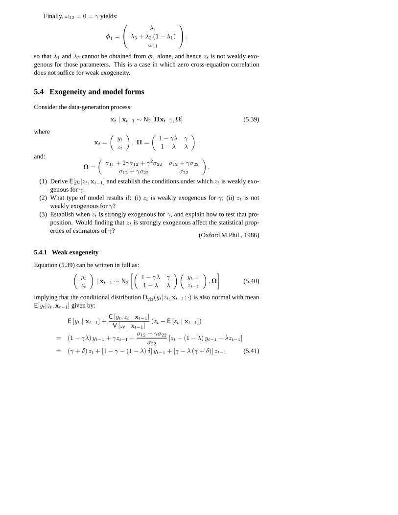
5.4 Exogeneity and model forms
Consider the data-generation process:
xt | xt−1 ∼ N2 [Πxt−1,Ω] (5.39)
where
xt =(
yt
zt
), Π =
(1 − γλ γ
1 − λ λ
),
and:
Ω =(
σ11 + 2γσ12 + γ2σ22 σ12 + γσ22
σ12 + γσ22 σ22
).
(1) DeriveE[yt|zt,xt−1] and establish the conditions under whichzt is weakly exo-genous forγ.
(2) What type of model results if: (i)zt is weakly exogenous forγ; (ii) zt is notweakly exogenous forγ?
(3) Establish whenzt is strongly exogenous forγ, and explain how to test that pro-position. Would finding thatzt is strongly exogenous affect the statistical prop-erties of estimators ofγ?
(Oxford M.Phil., 1986)
5.4.1 Weak exogeneity
Equation (5.39) can be written in full as:(yt
zt
)| xt−1 ∼ N2
[(1 − γλ γ
1 − λ λ
)(yt−1
zt−1
),Ω]
(5.40)
implying that the conditional distributionDy|z(yt|zt,xt−1; ·) is also normal with meanE[yt|zt,xt−1] given by:
E [yt | xt−1] +C [yt, zt | xt−1]V [zt | xt−1]
(zt − E [zt | xt−1])
= (1 − γλ) yt−1 + γzt−1 +σ12 + γσ22
σ22[zt − (1 − λ) yt−1 − λzt−1]
= (γ + δ) zt + [1 − γ − (1 − λ) δ] yt−1 + [γ − λ (γ + δ)] zt−1 (5.41)
whereδ = σ12σ−122 , and variance:
V [yt | xt−1] − C2 [yt, zt | xt−1]V [zt | xt−1]
= σ11 + 2γσ12 + γ2σ22 − (σ12 + γσ22)2
σ22
= σ11 − σ212
σ22:= σ2. (5.42)
Weak exogeneity requires two conditions to be satisfied: (i) the parameters of in-terest must be recoverable from the parametersφ1 of the conditional distribution alone,and (ii)φ1 and the parametersφ2 of the marginal distributionDz(zt|xt−1; ·) must bevariation free. So, to examine the conditions under whichzt is weakly exogenous forγ,we start by obtainingφ1 andφ2. Because normal distributions are completely specifiedby their first two moments, then (5.41) and (5.42) imply that:
φ1 =
γ + δ
1 − γ − (1 − λ) δ
γ − λ (γ + δ)σ2
= f
γ
δ
λ
σ2
.
In addition, because marginals of joint normals are also normal then:
zt | xt−1 ∼ N [(1 − λ) yt−1 + λzt−1, σ22] ,
and so:
φ2 =
1 − λ
λ
σ22
= g(
λ
σ22
).
There are several conditions under whichzt may be weakly exogenous forγ. First,note that (5.41) can be written as:
yt = (γ + δ) zt + [1 − γ − (1 − λ) δ] yt−1 + [γ − λ (γ + δ)] zt−1 + vt (5.43)
with:vt = yt − E [yt | zt,xt−1] ,
so that the conditional-marginal system can be written in general as:
∆yt = (γ + δ)∆zt − [γ + (1 − λ) δ] (yt−1 − zt−1) + γ (1 − λ) zt−1 + vt
∆zt = (1 − λ) (yt−1 − zt−1) + ε2,t (5.44)
whereε2,t is the second element inεt defined by:
εt = xt − E [xt | xt−1] .
The main cross linkage is(1 − λ), noting thatE[vtε2,s] = 0 ∀t, s as vt = ε1,t −(γ + δ) ε2,t.
(i) Considerσ12 = 0. If σ12 = 0, thenδ = 0, and hence:
φ1 =
γ
1 − γ
γ (1 − λ)σ11
= h
γ
λ
σ11
,
so thatγ can be obtained fromφ1 alone because it is just its first element.However,φ1 andφ2 are not variation free because(1 − λ) appears inφ1, whichimposes a restriction onφ1’s parameter space. Also,(1−λ) = φ1,3/φ1,1 therebyreducing the number of parameters requiring estimation in the system. The samerestriction is imposed when joint stationarity is required becauseδ = 0 impliesthat (5.44) is:(
∆yt
∆zt
)=( −γλ γ
1 − λ −(1 − λ)
)(yt−1
zt−1
)+(
ε1,t
ε2,t
),
so that the system is stationary if the matrix of coefficients in this system is fullrank which occurs ifγ 6= 0 andλ 6= 1.
(ii) Considerλ = 0, which implies that:
φ1 =
γ + δ
1 − γ − δ
γ
σ2
,
so thatγ is just the third element inφ1. Also, φ1 andφ2 are variation freeasφ2 = (σ22). Requirements of stationarity do not impose cross-restrictionsbetweenφ1 andφ2 because ifλ = 0, then (5.44) is:(
∆yt
∆zt
)=(
0 γ
1 −1
)(yt−1
zt−1
)+(
ε1,t
ε2,t
),
and so stationarity requiresγ 6= 0. Thus,λ = 0 implies thatzt is weakly exogen-ous forγ even if stationarity is required.
(iii) Considerλ = 1, then:
φ1 =
γ + δ
1 − γ
−δ
σ2
,
so thatγ can be obtained by adding the first and third elements. In addition,φ1
andφ2 are variation free if(γ, λ, σ11, σ12, σ22) are so. Stationarity cannot beimposed becauseλ = 1 implies that (5.44) is:
∆yt = (γ + δ) ∆zt − γ (yt−1 − zt−1) + ε1,t
∆zt = ε2,t (5.45)
so thaty andz are cointegrated with a unit coefficient, and the latter has a unitroot.
(iv) Whenγ = 0, δ 6= 0 then (5.44) is:(∆yt
∆zt
)= (1 − λ)
(0 01 −1
)(yt−1
zt−1
)+(
ε1,t
ε2,t
),
so thaty andz are cointegrated again. However, the first equation can also bewritten as:
∆yt = ε1,t = δε2,t + vt = δ∆zt − (1 − λ)δ(yt−1 − zt−1) + vt (5.46)
implying that the equilibrium correction occurs in both equations so thatzt cannotbe weakly exogenous for the parameters in the cointegration vector, and thereforeweak exogeneity is violated once more.
5.4.2 Resulting equations
Most of these have been noted above. If conditions for weak exogeneity are not im-posed, the conditional equation (5.43) is AD(1, 1). Reconsiderγ = 0, for example,which implies that (5.43) is in fact (5.46) and so it is an equilibrium-correction equa-tion with a long-run coefficient of1, wherezt is:
∆zt = (1 − λ) (yt−1 − zt−1) + ε2,t.
Hence the system is non-stationary, with a long-run solution ofy = z.
5.4.3 Testing for strong exogeneity and properties of estimators
Strong exogeneity requires weak exogeneity plus the absence of Granger causality. Letus considerλ = 1. If λ = 1, the distribution ofDz(zt|xt−1; ·) is:
zt | xt−1 ∼ N [zt−1, σ22] ,
and hencezt is independent of pastys, implying the absence of Granger causality.Hence,λ = 1 implies thatzt is strongly exogenous forγ. But λ = 1 also impliesthatzt is a random walk. Hence, testing for the absence of Granger causality may bethought to amount to testing whetherλ = 1 in the equation forzt, i.e., whether there isa unit root in the process generatingzt. However, as seen in (5.46), the two variableshave unit roots even when weak exogeneity is violated, so tests like Dickey–Fuller andSargan–Bhargava would not be testing for strong exogeneity ofzt for γ. In practice,economists test for Granger causality by testing for the significance of laggedys in thez equation. However, as we saw in§5.2.8, this procedure may not be robust to changesin the sample period examined, the selection of variables, or the number of lags in theregression.
Let us now look at the properties of theOLS estimator ofγ obtained from equation(5.45). Becauseλ = 1 implies thatzt is I (1), OLS is valid in equation (5.45a) asyt isalsoI(1) sinceyt andzt cointegrate:OLS has the usual properties of consistency andasymptotic normality.
5.5 Exogeneity and differencing
In the data-generation process:
xt | xt−1 ∼ N2 [Πxt−1,Ω] (5.47)
where:
xt =(
yt
zt
), Π =
(1 − γ + βµ γ − β (1 − λ)
µ λ
), Ω =
(ω11 ω12
ω12 ω22
)(5.48)
(1) DeriveE[yt|zt,xt−1], and establish the conditions under whichzt is weakly exo-genous for(γ, β).
(2) If ∆yt = yt − yt−1, and it is asserted by an investigator that∆yt = α∆zt + εt
whereE[∆ztεt] = 0 ∀t, what isplimT→∞ α (where˜ denotes a least-squaresestimator)? Under what conditions isα consistent forβ (you may assume thatthe latent roots ofΠ have modulus less than unity)?
(3) Comment on the formulation of the models in (5.47) and (5.48). Establish whenz does not Granger-causey, and explain how you would test that proposition.
(Oxford M.Phil., 1984)
5.5.1 Weak exogeneity
Equations (5.47) and (5.48) imply thatyt|zt,xt−1 is normally distributed with meanE[yt|zt,xt−1] given by:
E [yt | xt−1] +C [yt, zt|xt−1]V [zt|xt−1]
(zt − E [zt | xt−1])
= (1 − γ + βµ) yt−1 + [γ − β (1 − λ)] zt−1 +ω12
ω22(zt − µyt−1 − λzt−1)
= δzt + [1 − γ + (β − δ)µ] yt−1 + [γ − β + λ (β − δ)] zt−1 (5.49)
whereδ = ω12ω−122 , and variance:
V [yt | xt−1] − C2 [yt, zt|xt−1]V [zt|xt−1]
= ω11 − ω212
ω22:= ω2.
Thus, the parameters of the conditional distribution are:
φ1 =
δ
1 − γ + (β − δ) µ
γ − β + (β − δ)λ
ω2
= f
δ
γ
β
µ
λ
ω2
.
From the four coefficients, the six underlying parameters are not identifiable withoutadditional information. In addition, normality implies that:
zt | xt−1 ∼ N [µyt−1 − λzt−1, ω22] (5.50)
so that the parameters of this distribution are:
φ2 =
µ
λ
ω22
.
Together, these are sufficient to uniquely identify the seven original parameters.Forzt to be weakly exogenous for(γ, β) we require (i) to be able to recover(γ, β)
fromφ1 alone, and (ii)φ1 andφ2 to be variation free. Considerβ = δ. Then:
φ1 =
β
1 − γ
γ − β
ω2
,
so that,(γ, β) can be obtained fromφ1 alone. In addition,φ1 andφ2 are variation freeif (β, γ, µ, λ, ω11, ω12, ω22) are so. Hence,β = δ is sufficient for the weak exogeneityof zt for (γ, β). zt is weakly exogenous under stationarity because (5.47) can be writtenas: (
∆yt
∆zt
)=( −γ + βµ γ − β(1 − λ)
µ λ − 1
)(yt−1
zt−1
)+(
u1,t
u2,t
)(5.51)
where:
ut :=(
u1,t
u2,t
)= xt − E [xt | xt−1] . (5.52)
Stationarity requiresγ 6= 0 andµ + λ 6= 1 and so does not impose restrictions acrossφ1 andφ2.
5.5.2 Growth-rate models
TheOLS estimator ofα in the investigator’s model is defined as:
α =
(T∑
t=1
(∆zt)2
)−1 T∑t=1
∆zt∆yt.
To find itsplim, notice that (5.47) is the reduced form of:
yt = βzt + (1 − γ)yt−1 + (γ − β)zt−1 + η1,t
zt = µyt−1 + λzt−1 + u2,t,
so that:∆yt = β∆zt − γ (yt−1 − zt−1) + η1,t,
and:u1,t = η1,t + βu2,t,
so:∆yt = β∆zt − γ (yt−1 − zt−1) + u1,t − βu2,t. (5.53)
Hence:
α =
(T∑
t=1
(∆zt)2
)−1 T∑t=1
∆zt [β∆zt − γ (yt−1 − zt−1) + u1,t − βu2,t]
= β −(
T∑t=1
(∆zt)2
)−1 T∑t=1
∆zt [γ (yt−1 − zt−1) − u1,t + βu2,t] . (5.54)
Since (5.47) is the DGP, we takeut to be serially independent. Although the invest-igator may believe that she is estimating the impact coefficient of a differenced model,(5.53) reveals that the model is a reparameterized levels representation. Becausext isstationary and ergodic (see Hannan, 1970, p.203–4) thenyt−1zt, ztyt,
z2
t
, and
ztzt−1 are stationary and ergodic. In addition, becauseui,t ∼ IID, thenui,t isstationary and ergodic, and soztu1,t, zt−1u1,t, ztu2,t andzt−1u2,t all are sta-tionary and ergodic, andu1,tu2,t ∼ IID. Hence, the Ergodic and Slutsky’s theoremsimply that:
αAS→ β − γ
E [∆zt (yt−1 − zt−1)]
E[(∆zt)
2] +
E [∆zt (u1,t − βu2,t)]
E[(∆zt)
2] .
But, from (5.52),E[zt−1ui,t] = 0, (i = 1, 2) and by noticing that under weak exogen-eity β = δ thenu1,t − βu2,t is in fact the error in the conditional equation arising from(5.49). Hence,E[zt (u1,t − βu2,t)] = 0, (i = 1, 2) under weak exogeneity and so:
αAS→ β − γ
E [∆zt (yt−1 − zt−1)]
E[(∆zt)
2] .
The remaining term has to be calculated from the marginal distribution:
∆zt = µ (yt−1 − zt−1) − (1 − λ − µ) zt−1 + u2,t (5.55)
The simplest case isµ = 0, so changes inz are uncorrelated with past disequilibria,
and henceαAS→ β whenzt is also weakly exogenous for(β, γ). Alternatively, when
β = δ butµ = 1 − λ, then stationarity is violated and:
αAS→ β − γµ
E[(yt−1 − zt−1)
2]
µ2E[(yt−1 − zt−1)
2]
+ ω22
= β − γµ
µ2 + k,
wherek is the inverse signal-noise ratio:
k =ω22
E[(yt−1 − zt−1)
2] .
Thus, the inconsistency fromβ is less thanγ if µ/(µ2 + k) < 1. The outcome canbe calculated more generally from (5.53) and (5.55), but the algebra is tedious (themoments involve solving (5.35)+(5.36)). In practice, it is often found that the short-runimpact∆zt and the long-run effect(yt−1−zt−1) are not highly correlated, so that weakexogeneity yields an estimate ofα close toβ asT increases.
5.5.3 Strong exogeneity
The results obtained in§5.5.2 confirm that, in practice, it is difficult to detect mis-specifications in growth models.
Finally, zt is strongly exogenous for(γ, β) if β = δ andµ = 0 because the firstcondition implies weak exogeneity and the second the absence of Granger causality,since then the marginal distribution ofzt|xt−1 is:
zt | xt−1 ∼ N [λzt−1, ω22] ,
and so is independent of pastys. Testing this proposition would require adding laggedys to the marginal distribution and testing their significance. Although the process isthen stationary, the growth model delivers a consistent estimate of the impact effect of∆zt on∆yt.
5.6 Exogeneity in a trivariate process
Consider the three-dimensional vector random variablewt = (yt, xt, zt)′ with the jointdistributionDw(wt|wt−1;Π,Σ) given bywt|wt−1 ∼ N3 [Πwt−1,Σ] where:
Π =
0 α γ
0 δ θ
0 0 µ
and Σ =
σ11 σ12 σ13
σ12 σ22 σ23
σ13 σ23 σ33
.
(1) DeriveE[yt|zt,wt−1] andE[xt|zt,wt−1] as explicit functions of the paramet-ers (Π,Σ), whereE[·|·] denotes a conditional expectation. Also derive theconditional distribution ofut = (yt, xt)′, given zt and wt−1, denoted byDu|z,w(ut|zt,wt−1; ·).
(2) Define the concepts of weak and strong exogeneity. Consider the hypothesis that:
E [yt | zt,wt−1] = βE [xt | zt,wt−1] . (5.56)
What restrictions on the parameters ofΠ are imposed by (5.56)? Under what con-ditions on(Π,Σ) is zt weakly exogenous forβ in Du|z,w (ut|zt,wt−1; ·) when(5.56) is true?
(3) DeriveE [yt|xt,wt−1] as a function of the parameters(Π,Σ). Under what con-ditions, if any, on(Π,Σ) is xt weakly exogenous forβ when (5.56) is true?Comment on how reasonable such conditions might be when (5.56) correctly de-scribes agent behaviour.
(4) Is zt strongly exogenous forβ? Are there conditions under whichxt is stronglyexogenous forβ?
(Oxford M.Phil., 1991)
5.6.1 Conditional distributions
Becausewt|wt−1 ∼ N3 [Πwt−1,Σ], then conditionals from this joint distribution arenormal. Hence:
E [yt | zt,wt−1] = E [yt | wt−1] +C [yt, zt|wt−1]V [zt|wt−1]
(zt − E [zt | wt−1])
= αxt−1 + γzt−1 +σ13
σ33(zt − µzt−1)
= ρzt + αxt−1 + (γ − ρµ) zt−1 (5.57)
whereρ = σ−133 σ13. Next:
E [xt | zt,wt−1] = E [xt | wt−1] +C [xt, zt|wt−1]V [zt|wt−1]
(zt − E [zt | wt−1])
= δxt−1 + θzt−1 +σ23
σ33(zt − µzt−1)
= λzt + δxt−1 + (θ − λµ) zt−1 (5.58)
whereλ = σ−133 σ23. Finally,ut|zt,wt−1 is also normally distributed with:
E [ut | zt,wt−1] =(
E [yt|zt,wt−1]E [xt|zt,wt−1]
)=
(ρzt + αxt−1 + (γ − ρµ) zt−1
λzt + δxt−1 + (θ − λµ) zt−1
)(5.59)
and:
V [ut | zt,wt−1] = V
[(yt
xt
)| wt−1
]− C [ut, zt|wt−1] C [ut, zt|wt−1]
′
V [zt|wt−1]
=(
σ11 σ12
σ21 σ22
)− 1
σ33
(σ13
σ23
)(σ13 σ23
)
=
σ11 − σ213
σ33σ12 − σ13σ23
σ33
σ12 − σ13σ23
σ33σ22 − σ2
23
σ33
(5.60)
=(
ω11 ω12
ω12 ω22
).
5.6.2 Weak exogeneity in a bivariate distribution
A variablezt is weakly exogenous for a parameters of interestψ if the following twoconditions are satisfied:
(i) ψ is a function of the parametersφ1 of the conditional distribution alone; and(ii) φ1 and the parametersφ2 of the marginal distribution are variation free.
A variablezt is strongly exogenous forψ if:
(i) zt is weakly exogenous forψ; and(ii) y does not Granger causez.
To find what restrictions are imposed onΠ by (5.56), let us replace expectations in(5.56) by their expressions in (5.57) and (5.58):
ρzt + αxt−1 + (γ − ρµ) zt−1 = β (λzt + δxt−1 + (θ − λµ) zt−1) ,
so that:ρ = βλ, α = βδ and γ − ρµ = β (θ − λµ) .
Substituting the first equality into the third yields:
γ − βλµ = βθ − βλµ,
or:γ = βθ.
Hence, (5.56) imposes the following restrictions onΠ: α = βδ andγ = βθ.To analyze the weak exogeneity ofzt for β, we write down the parameters of
the appropriate conditional and marginal distributions. First, we show thatzt is
not weakly exogenous forβ in (5.56) written asyt = βE[xt|zt,wt−1] + vt withvt = yt − E [yt|zt,wt−1]. Write the conditional model as:
yt = E [yt | zt,wt−1] + vt
= βE [xt | zt,wt−1] + vt
= βλzt + βδxt−1 + β (θ − λµ) zt−1 + vt,
where:
V [yt | zt,wt−1] = σ11 − σ213
σ33:= ω11 = V [vt] .
Thus, when (5.56) is true:
φ′1 =
(βλ βδ β (θ − λµ) ω11
)=
(βλ α γ − βλµ ω11
)= f
(β α λ µ γ ω11
).
Even with the parametric restrictions,β is not identifiable from this conditional distri-bution alone. In addition, becausezt|wt−1 ∼ N[µzt−1, σ33] then:
φ2 =(
µ
σ33
).
Even learningµ from φ2 will not identify β: the process generatingxt is germane tothe determination of the parameters using:
xt = λzt + δxt−1 + (θ − λµ) zt−1 + et,
with:et = xt − E[xt | zt,wt−1],
from which λ, δ, andθ − λµ can be obtained. Thus, the joint bivariate distributionDu|z,w(ut|zt,wt−1; ·) must be analyzed, and the issue concerns the weak exogeneity ofzt in that joint.
From (5.59):
E
[(yt
xt
)| zt,wt−1
]=
(ρzt + αxt−1 + (γ − ρµ) zt−1
λzt + δxt−1 + (θ − λµ) zt−1
),
which together with (5.60) implies:
φ′1 =
(ρ α γ − ρµ λ δ (θ − λµ) ω11 ω12 ω22
)=
(βλ βδ β (θ − λµ) λ δ (θ − λµ) ω11 ω12 ω22
),
usingρ = βλ, α = βδ andγ = βθ. Examiningφ1, we notice thatβ can be obtained asthe ratio of the first to the fourth element inφ1, or second to fifth, or third to sixth, so
that it can be obtained fromφ1 alone. Hence, the first condition for weak exogeneityof zt for β is satisfied. In addition, althoughµ appears inφ1, sinceθ andλ are notrestricted,φ1 andφ2 are variation free if all parameters are so. Hence,zt is weaklyexogenous forβ. To achieve super exogeneity ofzt for β, however,θ = λµ is required,in which case,zt−1 does not enter the conditional joint distribution.
Parameters are variation free even if stationarity is required. To see this, we firstfind the stationarity conditions. The system is stationary if the eigenroots ofΠ are allinside the unit circle. The eigenroots are the solution forξ to the following equation:
det
−ξ α γ
0 δ − ξ θ
0 0 µ − ξ
= 0,
or to:−ξ (δ − ξ) (µ − ξ) = 0,
which implies that:ξ = µ; ξ = δ; ξ = 0.
Hence, for stationarity we require|µ| < 1 and |δ| < 1. Thus, even if|µ| < 1, theelements ofφ1 depending uponµ can vary anywhere, and soφ1 andφ2 are variationfree. Hence, no conditions additional to those imposed by (5.56) are needed forzt tobe weakly exogenous forβ.
5.6.3 Feedback versus feedforward models
Now:
E [yt | xt,wt−1] = E [yt | wt−1] +C [yt, xt|wt−1]V [xt|wt−1]
(xt − E [xt | wt−1])
= αxt−1 + γzt−1 +σ12
σ22(xt − δxt−1 − θzt−1)
= ηxt + (α − δη) xt−1 + (γ − ηθ) zt−1 (5.61)
whereη = σ12σ−122 , and:
V [yt | xt,wt−1] = σ11 − σ212
σ22:= σ2,
so that:
φ1 =
η
α − δη
γ − ηθ
σ2
.
Also:xt | wt−1 ∼ N [δxt−1 + θzt−1, σ22] ,
and so:
φ2 =
δ
θ
σ22
.
But (5.56) implies thatα = βδ andγ = βθ, and so:
φ1 =
η
(β − η) δ
(β − η) θ
σ2
.
Hence,β = η is a sufficient condition for the weak exogeneity ofxt for β because thenφ1 =
(β, σ2
)′, soβ can be recovered fromφ1 alone, andφ1 andφ2 are variation free.
To analyze how sensible the conditions implied by (5.56) are, notice that:
m1 = E [yt | wt−1] = αxt−1 + γzt−1,
and:m2 = E [xt | wt−1] = δxt−1 + θzt−1,
so thatα = βδ andγ = βθ imply that:
m1 = βδxt−1 + βθzt−1 = βm2.
Thus, the implicit plan linking the conditional expectations yields a proportional rela-tion, compatible with some equilibrium economic theories. Also, under those condi-tions, (5.61) is:
E [yt | xt,wt−1] = ηxt + δ (β − η) xt−1 + θ (β − η) zt−1,
which can be written as:
yt = ηxt + δ (β − η)xt−1 + θ (β − η) zt−1 + εt (5.62)
with:εt = yt − E [yt | xt,wt−1] ,
so that from (5.62):
E [yt | zt,wt−1] = ηE [xt | zt,wt−1] + δ (β − η) xt−1
+θ (β − η) zt−1 + E [εt | zt,wt−1] .
Thus, interpreting the coefficient ofxt asβ in this equation will be incorrect unlessβ = η, i.e., unlessxt is weakly exogenous forβ andεt is an innovation againstzt.This corresponds to a contingent plan model (see 6), rather than an expectations-basedrelation. In other words, (5.56) is derived from taking conditional expectations withrespect to(zt,wt−1) in the model:
yt = βxt + wt.
5.6.4 Strong exogeneity
We have found in§5.6.2 thatzt is weakly exogenous forβ. In addition, becausezt|wt−1 ∼ N[µzt−1, σ33], then it is independent of pastys andxs. So,zt is stronglyexogenous forβ. We have also found in§5.6.3 thatxt is weakly exogenous forβif β = σ12σ
−122 , so under that condition,xt is strongly exogenous forβ because the
distributionxt|wt−1 ∼ N[δxt−1 + θzt−1, σ22] is also independent of pastys.
5.7 Exogeneity in a non-constant process
Consider the following DGP wherext = (yt : zt)′:
xt | xt−1 ∼ N2 [Πxt−1,Ωt] (5.63)
where:
Π =(
γ + βµ β(λ − γ)µ λ
)and Ωt =
(ω11,t ω12,t
ω21,t ω22,t
).
(1) WhenΩt = Ω is constant over time in (5.63), obtainE[yt|zt,xt−1]. Derive theconditional densityDy|z(yt|zt,xt−1). Show that its error varianceσ2 is neverlarger thanω11.
(2) KeepingΩ constant and assuming that the parameters(β, γ, λ, µ, ω11, ω12, ω22)are all variation free beyondΩ being positive definite, establish conditions underwhich zt is weakly exogenous forβ. What type of model results ifzt is weaklyexogenous forβ? Which parameters determine the short-run, and which the long-run, response ofyt to zt?
(3) WhenΩt is not constant, deriveE[yt|zt,xt−1]. Is β invariant to changes in themarginal distribution ofzt? Establish conditions under whichzt is super exo-genous for
(β, σ2
).
(4) Whenω12,t = 0: (i) is zt predetermined inE[yt|zt,xt−1]? (ii) canzt be superexogenous for the parameter vector (denotedδ) of E[yt|zt,xt−1] for changes inthe parameters of the marginal distribution?
(Oxford M.Phil., 1992)
5.7.1 Variance dominance in constant processes
Becausext|xt−1 ∼ N2[Πxt−1,Ωt], thenyt|zt,xt−1 is also normally distributed withmeanE[yt|zt,xt−1] given by:
E [yt | xt−1] +C [yt, zt|xt−1]V [zt|xt−1]
(zt − E [zt | xt−1])
= (γ + βµ) yt−1 + β(λ − γ)zt−1 +ω12
ω22(zt − µyt−1 − λzt−1)
= αzt + [γ + (β − α)µ] yt−1 + [−βγ + (β − α)λ] zt−1 (5.64)
whereα = ω12ω−122 , and variance:
V [yt | zt,xt−1] = V [yt | xt−1] − C2 [yt, zt|xt−1]V [zt|xt−1]
= ω11 − ω212
ω22:= σ2.
That the conditional variance cannot be greater than the unconditional can be seen bynoticing thatω2
12 ≥ 0, and asω11 andω22 are variances, so must be non-negative, thentω11 ≥ σ2.
5.7.2 Statistical validity of COMFAC models
zt is weakly exogenous forβ if the following two conditions are satisfied: (i)β canbe obtained from the parametersφ1 of the conditional distribution alone, and (ii)φ1
and the parametersφ2 of the marginal distributionzt|xt−1 are variation free. Becausemarginals of joint normal densities are also normal:
zt | xt−1 ∼ N [µyt−1 + λzt−1, ω22] ,
so that the parameters of the conditional and marginal distributions are:
φ1 =
α
γ + (β − α)µ
−βγ + (β − α)λ
σ2
and φ2 =
µ
λ
ω22
,
respectively. Hence, ifβ = α:
φ1 =
β
γ
−βγ
σ2
,
soβ can be recovered fromφ1 alone. Because the parameters(β, γ, λ, µ, ω11, ω12, ω22)are all variation free by assumption, thenφ1 andφ2 are variation free. Hence,β = α
is a sufficient condition forzt to be weakly exogenous forβ.Because (5.64) can also be written as the conditional equation:
yt = αzt + [γ + (β − α)µ] yt−1 + [−βγ + (β − α)λ] zt−1 + νt,
with:νt = yt − E [yt | zt,xt−1] ,
then, under the condition for weak exogeneity, i.e.,β = α, the conditional equation is:
yt = βzt + γyt−1 − βγzt−1 + νt, (5.65)
which can also be written as:
yt = βzt + ut
ut = γut−1 + νt,
and so is a COMFAC model. Hence, althoughβ = α allows us to estimate (5.65)without loss of information, the resulting equation only has the economic theory inter-pretation of ‘bad luck–good luck’ operating, since the agents make no effort to correctthe resulting disequilibria. By writing (5.65) as:
yt = βzt + γut−1 + νt,
we could interpret such an equation as if either previous autonomous shocks directlyaffect currentys, or alternatively as if agents adjust for autonomous shocks as well asfor changes inz. A property of this kind of equation is that short-run and long-runeffects are equal. The short run effect ofz on y is defined as∂yt/∂zt and so equalsβ. The long-run effect is defined by
∑∞i=0 wi, wherewi is the ith coefficient in the
polynomial obtained by writingyt in terms ofz and lags thereof only. So, to computethe long-run effect, we write (5.65) in terms of the lag operator as follows:
(1 − γL) yt = β (1 − γL) zt + νt,
or:yt = βzt + (1 − γL)−1
νt,
so that the long-run effect ofz on y is alsoβ. Hence,β determines both short-run andlong-run responses ofy to z.
5.7.3 Super exogeneity in non-constant processes
WhenΩt is non-constant, thenE[yt|zt,xt−1] is given by:
ω12,t
ω22,tzt +
[γ +
(β − ω12,t
ω22,t
)µ
]yt−1 +
[−βγ +
(β − ω12,t
ω22,t
)λ
]zt−1
= βzt + (αt − β) (zt − µyt−1 − λzt−1) + γyt−1 − βγzt−1,
whereαt = ω12,tω−122,t and:
V [yt | zt,xt−1] = ω11,t −ω2
12,t
ω22,t:= σ2
t ,
so that:
φ1,t =
αt
γ + (β − αt) µ
−βγ + (β − αt)λ
σ2t
and φ2,t =
µ
λ
ω22,t
.
Then,β is invariant to changes in the marginal distribution ofzt, if it is invariant to in-terventions onµ, λ andω22,t. So, ifω12,t = βω22,t, thenβ is invariant to interventionsonφ2,t, i.e.,αt = β ∀t.
For zt to be super exogenous for(β, σ2
t
)the following two conditions must be
satisfied: (i)zt must be weakly exogenous for(β, σ2
t
)and (ii)φ1,t must be invariant
to interventions onφ2,t. Hence,ω12,t = βω22,t is a sufficient condition for weakexogeneity because then:
φ1,t =
β
γ
−βγ
σ2t
,
so(β, σ2
t
)can be recovered fromφ1,t alone, andφ1,t andφ2,t are variation free. If, in
addition:
ω11,t −ω2
12,t
ω22,t= ω11,t − βω12,t := σ2,
soω11,t changes to compensate for potential changes inω12,t, thenφ1 is fully invariantto interventions onφ2,t, and hencezt is super exogenous for
(β, σ2
).
5.7.4 Predeterminedness and super exogeneity
Whenω12,t = 0, then:
E [yt | zt,xt−1] = (γ + βµ) yt−1 + β (λ − γ) zt−1,
yielding the following conditional equation:
yt = (γ + βµ) yt−1 + β (λ − γ) zt−1 + vt. (5.66)
But (5.63) can also be written as:(yt
zt
)=(
γ + βµ β (λ − γ)µ λ
)(yt−1
zt−1
)+(
u1,t
u2,t
)(5.67)
with:
ut =(
u1,t
u2,t
)= xt − E [xt | xt−1] (5.68)
so by comparing (5.66) and (5.67), we notice thatvt = u1,t, and hence (5.66) is:
yt = (γ + βµ) yt−1 + β (λ − γ) zt−1 + u1,t. (5.69)
We now check whetherzt is predetermined in (5.69). Forzt to be predetermined in(5.69),E[zt−iu1,t] must equal zero for alli ≥ 0. Proving thatE[ztu1,t] = 0 is straight-forward because (5.68) impliesE[yt−1u1,t] = E[zt−1u1,t] = 0, and so:
E [ztu1,t] = E [(µyt−1 + λzt−1 + u2,t)u1,t]
= µE [yt−1u1,t] + λE [zt−1u1,t] + E [u2,tu1,t] = 0,
if ω12,t = 0. Under stationarityE[zt−iu1,t] = E[ztu1,t+i]. To find these expectations,write zt in terms of laggedus. From (5.67):(
yt
zt
)=
(1 − (γ + βµ) L −β (λ − γ)L
−µL 1 − λL
)−1
ut
= h (L)(
1 − λL β (λ − γ)L
µL 1 − (γ + βµ)L
)ut,
where:
h (L) =1
1 − (λ + γ + βµ) L + γ (λ + βµ)L2,
so denoting byξi (i = 1, 2) the roots of the polynomial:
ξ2 − (λ + γ + βµ) ξ + γ (λ + βµ) = 0,
whenξ1 6= ξ2:
zt =1
ξ1 − ξ2
(1
1 − ξ1L− 1
1 − ξ2L
)[µu1,t + u2,t+1 − (γ + βµ)u2,t]
=1
ξ1 − ξ2
∞∑j=0
(ξj1 − ξj
2
)[µu1,t−j + u2,t−j+1 − (γ + βµ) u2,t−j] .
Hence, when theus are serially uncorrelatedE[ztu1,t+i] = 0 for all i > 0.
Often,ω12,t = 0 is also sufficient for valid inference. However, here under thatcondition:
φ1,t =
γ + βµ
β (λ − γ)ω11,t
,
so thatzt cannot be weakly exogenous forβ, asβ cannot be recovered fromφ1,t alone,and hencezt cannot be super exogenous. In addition,φ1,t is not invariant to changesin φ2,t because changes inµ andλ (both being parameters of the marginal distribu-tion) will induce changes in(γ − βµ) and inβ (λ − γ) except whenβ = 0. Thus,predeterminedness and strict exogeneity do not sustain inference about the parametersof interest in this example, and even lose the crucial property of invariance.
5.8 Exogeneity in a cointegrated process
Consider the following bivariate DGP for theI(1) vectorxt = (yt : zt)′:
yt = βzt + ε1,t
∆zt = λ∆yt−1 + ρ (yt−1 − βzt−1) + ε2,t(5.70)
whereεt = (ε1,t : ε2,t)′ is distributed as in (5.71):(
ε1,t
ε2,t
)∼ IN2
[(00
),
(σ2
1 γσ1σ2
γσ1σ2 σ22
)]:= IN2 [0,Σ] . (5.71)
The parameters(β, σ1; λ, ρ, γ, σ2) in (5.70) and (5.71) are all variation free beyond therequirement thatΣ is positive definite; the parameter of interest isβ.
(1) Derive the conditional expectationE[yt|zt,Xt−1] of yt given (zt,Xt−1), andthe sequential densityDy|z(yt|zt,Xt−1; ·). Under what conditions iszt weaklyexogenous forβ?
(2) Explain the role ofγ in this system, and what relation, if any, it has to the weakexogeneity ofzt for β. Briefly describe how to test the weak exogeneity ofzt forβ.
(3) Under what conditions iszt strongly exogenous forβ? Whenzt is weakly exo-genous forβ, explain how to test for Granger causality of∆y on ∆z. Whatproblems arise in testing for Granger causality ofy on z whenzt is not weaklyexogenous forβ.
(Oxford M.Phil., 1993)
5.8.1 Weak exogeneity
System (5.70) can also be written as:(yt
zt
)=(
β (λ + ρ) −βλ β (1 − ρβ)λ + ρ −λ 1 − ρβ
) yt−1
yt−2
zt−1
+(
ε1,t + βε2,t
ε2,t
),
so normality implies that:(yt
zt
)| Xt−1 ∼ N2
( β (λ + ρ) −βλ β (1 − ρβ)λ + ρ −λ 1 − ρβ
) yt−1
yt−2
zt−1
,Ω
,
whereXt−1 only comprises(yt−1, yt−2, zt−1), and:
Ω =(
σ21 + 2βγσ1σ2 + β2σ2
2 γσ1σ2 + βσ22
γσ1σ2 + βσ22 σ2
2
).
Hence the conditional distribution ofyt|zt, yt−1, yt−2, zt−1 is also normal with meanE[yt|zt−1
t ,yt−2t−1] given by:
E[yt | yt−2
t−1, zt−1
]+
C[yt, zt|yt−2
t−1, zt−1
]V[zt|yt−2
t−1, zt−1
] (zt − E
[zt | yt−2
t−1, zt−1
])= β (λ + ρ) yt−1 − βλyt−2 + β (1 − ρβ) zt−1
+(
β +γσ1
σ2
)[zt − (λ + ρ) yt−1 + λyt−2 − (1 − ρβ) zt−1]
= (β + δ) zt − (λ + ρ) δyt−1 + λδyt−2 − (1 − ρβ) δzt−1 (5.72)
whereδ = γσ1/σ2, and conditional varianceV[yt|zt, yt−1, yt−2, zt−1] given by:
V[yt | yt−2
t−1, zt−1
]− C2[yt, zt|yt−2
t−1, zt−1
]V[zt|yt−2
t−1, zt−1
]= σ2
1 + 2βγσ1σ2 + β2σ22 −
(γσ1σ2 + βσ2
2
)2σ2
2
=(1 − γ2
)σ2
1 .
To find conditions for the weak exogeneity ofzt for β, we write down the parametersof this conditional distribution:
φ1 =
β + δ
− (λ + ρ) δ
λδ
− (1 − ρβ) δ(1 − γ2
)σ2
1
,
and notice that the marginal distributionzt|yt−1, yt−2, zt−1 is:
zt | yt−1, yt−2, zt−1 ∼ N[(λ + ρ) yt−1 − λyt−2 + (1 − ρβ) zt−1, σ
22
](5.73)
so that its parameters are:
φ2 =
λ + ρ
−λ
1 − ρβ
σ22
.
We will be able to recoverβ fromφ1 in several settings. First, ifγ = 0, thenδ = 0 andso:
φ1 =(
β
σ21
),
so β is just the first element inφ1. However,φ1 andφ2 are not variation free, eventhough all parameters were assumed to be so, becauseβ can be obtained fromφ2 as(1 − φ23)/(φ21 − φ22), and is the central parameter of interest. Hence,γ = 0 is nota sufficient condition for the weak exogeneity ofzt for β. BecauseV[ε1,t] = σ2
1 andV[ε2,t] = σ2
2 , thenE[ε1,tε2,t] = γσ1σ2 implies thatγ is the correlation betweenε1,t andε2,t. Consequently, this is an example in which zero cross-equation correlation does notsuffice for weak exogeneity.
Secondly, writing the system in (5.70) as:
∆yt = −(1 − ρβ)(yt−1 − βzt−1) + βλ∆yt−1 + ε1,t + βε2,t
∆zt = ρ(yt−1 − βzt−1) + λ∆yt−1 + ε2,t,
suggests consideringρ = 0 because then the long-run relationship enters the first equa-tion only. However,ρ = 0 implies:
φ1 =
β + δ
−λδ
λδ(1 − γ2
)σ2
1
and φ2 =(
λ
σ22
),
so that, althoughβ does not enter the marginal distribution, it cannot be recovered fromφ1 alone. The additional condition thatδ = 0 is needed, so there is no cross covariance.
5.8.2 Testing for weak exogeneity
Testing for the validity of exogeneity assumptions is important in econometric model-ling, but not always feasible. Four distinct failures of weak exogeneity can be delin-eated. First, if parameters other than those of interest (denotedψ) are delivered by theconditional model, then conditioning is invalid: examples include errors-in-variablesand simultaneity, in both of which the postulated conditional model does not deliverψ.Secondly, there are cases where inference is distorted even thoughψ is obtained: thissituation can occur in unit-root processes whereφ1 andφ2 both determineψ. Thirdly,knowledge ofφ2 may be essential to identifyψ, so conditioning is valid but unhelp-ful, in that the joint distribution has to be modelled to obtainψ. Finally, efficiencycan be lost if there is useful information inφ2 aboutφ1: an example is cross-equationrestrictions where ignoringφ2 does not induce inconsistency or inference distortions.
The role ofγ has been explained in§5.8.1. To test for weak exogeneity, write (5.72)as:
∆yt = (β + δ)∆zt − (1 + ρδ) (yt−1 − βzt−1) − λδ∆yt−1 + νt (5.74)
with:
νt = yt − E [yt | zt, yt−1, yt−2, zt−1] ,
and:
∆zt = λ∆yt−1 + ρ (yt−1 − βzt−1) + ε2,t. (5.75)
Expressed in this form, the system has one cointegrating relationshipyt−1 − βzt−1,andyt, zt areI (1) by assumption so that all variables are in anI (0) form and hence‘ t-tests’ have their usual distribution. Becauseρ = 0 andλδ = 0 jointly suffice forweak exogeneity, we must test for both long-run weak exogeneity (ρ = 0), and if that issatisfied, test for short-run (δ = 0). The first can be conducted as a test in the marginalmodel (5.75), once the determination of the cointegration parameterβ is done in thejoint distribution. Ifρ = 0, then testingλδ = 0 follows as the coefficient of∆yt−1 inthe conditional model. A joint test is more complicated.
5.8.3 Strong exogeneity
Strong exogeneity requires weak exogeneity plus the absence of Granger causality.We have discussed the conditions for weak exogeneity above. If these are satisfied,then Granger non-causality needs the marginal distributionzt|yt−1, yt−2, zt−1 to beindependent of pastys. From (5.73), a sufficient condition for this to occur is thatλ = ρ = 0. But, this condition implies that:
∆zt = ε2,t.
Thus, a test for strong exogeneity can be conducted by testing whether lagged∆ysand the cointegrating vector enter the marginal model. Of course,λ = 0 implies thatλδ = 0 and hence ensures weak exogeneity ifρ = 0. In this parameterization,γaffects the coefficients’ interpretation, but plays no role in determining weak or strongexogeneity.
However, even ifρ = 0, γ = 0 by itself is not sufficient for strong exogeneity whenλ 6= 0, although it does ensure weak exogeneity.
More subtle problems arise in testing for Granger causality whenzt is not weaklyexogenous forβ. First,λδ 6= 0 by itself precludes inference without loss of informationfrom the conditional model, but ifρ = 0, the standard test for the absence of Grangercausality in the marginal model holds. Conversely, ifρ 6= 0, there is Granger causality,as is the case whenλ 6= 0. Thus, a joint test of the role of∆yt−1 and(yt−1 − βzt−1) isneeded (see Toda and Phillips, 1993, for a discussion of some of the issues that arise).