77

5 – MODERN PORTFOLIO THEORY

Modern portfolio Theory (MPT) is one of the most important and influential economics

theories that deal with finance and investments. The Modern Portfolio Theory was

developed by Harry Markowitz (born August 24, 1927) and was published in 1952 in the

journal of finance under the name of “Portfolio Selection”. Later in 1959, He also

published a book by the name of “Portfolio Selection: Efficient Diversification of

Investments”. Decades later in 1990 he received Sveriges Riksbank Nobel Prize in

Economic Sciences for this work. What Harry Markowitz started back in the early 1960s

was continued through the development of the capital market theory, whose final

product, the capital asset pricing model (CAPM), allowed a Markowitz efficient investor

to estimate the required rate of return for any risky asset (Markowitz, 1990). The

Markowitz-Model is based on an ex-ante-perspective which means that for each

investment the expected return (mean) and the standard deviation as dispersion

measure around the mean should be estimated. In practice, it is however often

impossible to determine the probabilities of the return distribution. Therefore, an

assumption is made that the data of the past is valid for the future.

The introduction of modern portfolio theory by Harry Markowitz has led to a

mathematical explanation of the expression “don’t put all your eggs in one basket”

(Markowitz (1952)). One of the most fundamental conclusions in Markowitz‟ portfolio

choice theory is that rational investors should not choose assets only because of their

unique properties such as the expected return and variance, but should also consider

the covariation between the different assets. As the number of assets in a portfolio

increases, the covariance increasingly makes up a greater part of an individual assets

contribution to the total risk of a portfolio.

Basically, what MPT says is that, it is not enough to take only one particular asset’s risk

and return under consideration but rather investing in several assets with low

correlations towards each other. This will give the portfolio advantages of

diversification. Hence, the relevant objective in the MPT concept is to chose the right

combination (or proportions) of these assets to the optimal portfolios. This problem is

solved with the Mean-variance optimization model.

78

For each incremental asset, 1 variance term and n-1 covariance terms are added to the

matrix. As long as an asset does not correlate perfectly with the other assets in the

portfolio, the total variance will be reduced. From an investment perspective, this sheds

light on the benefits of diversification. The idea is that a portfolio should consist of a

large amount of assets, belonging to different lines of business with the purpose of

spreading the risk exposure while achieving lower correlation. The effect of

diversification is common knowledge within the field of financial theory and a great

number of researchers have found supporting evidence. Among these studies, Solnik

(1974) shows that the risk of a well-diversified portfolio initially decreases dramatically

and then converges to an undiversifiable level of risk, i.e. systematic risk. By using the

optimization procedure for a given universe of securities, an efficient frontier of risky

assets may be formed. The portfolios on the frontier are efficient in the sense that they

offer the highest return for any given level of risk. The optimization model follows the

Markowitz framework and models the rate of return on assets as random variables. The

optimization is done by choosing the weights of each asset in the portfolio optimally as

to minimize the portfolio volatility at any given rate of return on the portfolio

(Markowitz, 1952).

The risk reduction benefit of diversification is an important ideology of finance.

However, diversification studies typically employ only stocks and bonds (Satyanarayan

& Varangis 1996). Many studies have been carried out in the context of international

markets on the benefits of adding commodities to enhance equity diversification

(typically only using a commodity index or one category of futures to reduce risks), but

on the other hand a meticulous study is conspicuously missing in the context of Indian

markets. As commodity futures prices are influenced by factors different from those

that affect financial assets, commodity futures are perceived to be excellent candidates

for the diversification of equity and bond portfolios (Schneeweis, Savanayana, and

McCarthy 1991).

As said in economics, all economic decisions face trade-offs because of scarce resources

and Markowitz identified the trade-offs facing investors, which is risk versus expected

79

return. Prior to Markowitz’s work investors use to focus on the risks and returns on

individual securities when forming their portfolios. Generally investors were advised to

look for those securities that gave the best returns with the least risk. When those

securities were found, the investor was supposed to form a portfolio with weights in

these securities. This strategy might result in a portfolio purely formed of securities in

the same industry. Let’s for example say that the railroad industry was performing

really well, with regards to return and risk. In that case the investor would invest in

railroad securities.

The MPT, on the other hand, focuses on examining the risk-rewards characteristics of a

portfolio rather than on individual securities. Investors should not hold single asset,

they should hold groups or portfolios of assets. By holding portfolios of assets, the

investor might be able to obtain diversification, where he would get lower risk of his

portfolio of assets than of any individual assets (Bodie et.al 2009).

The objective behind MPT is to select a portfolio of various financial assets with the

highest expected return for a given amount of portfolio risk or equivalently to select a

portfolio with the lowest risk for certain level of portfolio expected return. Later, Tobin

(1958) extended Markowitz’s model by adding a risk-free rate to the model. With the

addition of the riskless rate he discovered that the efficient frontier turned out to be a

straight line where investors were now allowed to leverage their portfolio by short

selling the risk-free rate and buy more share in the market portfolio, or de-leverage by

selling some share of the market portfolio and invest in the risk-free asset. Tobin’s work

simplified the portfolio selection greatly since he discovered that every investor should

hold the same portfolio of risky assets. William Sharpe introduced in 1964 the Capital

Asset Pricing Model (CAPM) which identifies systematic and non systematic risk where

systematic risk is non-diversifiable and non-systematic risk can be diversified away by

increasing the number of stocks in portfolio.

The efficient frontier the minimum variance portfolio, tangency portfolio and the

optimal utility maximizing portfolio are developed and later a risk-free asset is added to

the model.

80

5.1 -MEAN VARIANCE OPTIMIZATION

Markowitz introduced Mean Variance theory for finding optimum portfolio of risky

assets, based on presumption that distribution of portfolio returns is normal and thus

can be successfully described by two moments – mean and variance. Mean – Variance

theory was further developed by Sharpe (e.g. Sharpe [1966], [1994], [2000]) and

extended to the theory of optimum portfolio selection to the whole market (macro)

perspective. Sharpe [1964] developed Capital Asset Pricing Model (CAPM), which is still

used by practitioners and serves as a cornerstone for a variety of portfolio selection

computer optimizers.

Sharpe [1966] focused on development of hedge fund model, which determinates a

portfolio with highest reward-to-variability ratio. Generally speaking, he developed a

theoretical concept for picking the portfolio which yields the highest return over the

unit of risk.

The mean-variance portfolio optimization theory of Markowitz (1952, 1959) is widely

regarded as one of the major theories in financial economics. It is a single-period theory

on the choice of portfolio weights that provide optimal tradeoff between the mean and

the variance of the portfolio return for a future period. Mean-variance optimization

(MVO) refers to a mathematical process that calculates the security or asset class

weights that provide a portfolio with the maximum expected return for a given level of

risk; or, conversely, the minimum risk for a given expected return. The inputs needed to

conduct MVO are security expected returns, expected standard deviations, and

expected cross-security correlations.

When first developed, mean-variance optimization was applied (if at all) only to

portfolios of individual stocks. Today, this technique is applied with increasing

frequency on an asset class level. This trend is appropriate for two reasons. First, the

inputs required by the Markowitz model are more difficult to estimate for individual

securities than they are for asset classes. Second, the range of asset classes available to

81

investors is now much larger, especially given the increased willingness of investors to

consider global investing (Lummer & Riepe 1994)

The consequence of mean-variance optimization is a set of asset class weights that can

be used as a long term guide for investing. This is often described as the portfolio’s

strategic asset allocation plan. The portfolio weights should be updated occasionally to

reflect changes in estimates of the long-term parameters or different needs of the

portfolio.

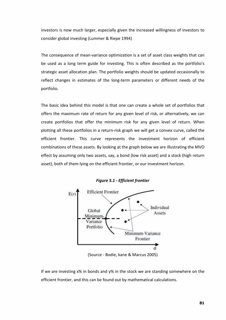
The basic idea behind this model is that one can create a whole set of portfolios that

offers the maximum rate of return for any given level of risk, or alternatively, we can

create portfolios that offer the minimum risk for any given level of return. When

plotting all these portfolios in a return-risk graph we will get a convex curve, called the

efficient frontier. This curve represents the investment horizon of efficient

combinations of these assets. By looking at the graph below we are illustrating the MVO

effect by assuming only two assets, say, a bond (low risk asset) and a stock (high return

asset), both of them lying on the efficient frontier, or our investment horizon.

Figure 5.1 - Efficient frontier

(Source - Bodie, kane & Marcus 2005)

If we are investing x% in bonds and y% in the stock we are standing somewhere on the

efficient frontier, and this can be found out by mathematical calculations.

82

If we change these proportions to, say, 10%, we are going to stand somewhere further

to the left on the frontier, with 90% bond and 10% stock. If we keep changing these

proportions in the same manner we will lower our risk until a certain point where the

risk starts to increase again. Conversely, this is called the diversification of unsystematic

risk. You can notice that the risk is not eliminated fully due to the systematic part of the

risk. The extent of how far we can diversify and eliminate unsystematic risk is

determined by the correlation coefficient. The lower the coefficient is between these

two assets, the more we will be able to diversify “and stretch the frontier curve towards

the y-axis”. In an unrealistic extreme case of, say, a correlation between these two

assets being -1, then we would end up with two linear straight lines where both have

the same y-intercept and different slopes. We would have then diversified away all the

risk. However, in this study we have different asset classes of equity and commodities

indidces and they are already diversified. The idea is still the same but more complex.

We will solve for this by using computer quadratic solving. (Brown et al, 2007, p.77).

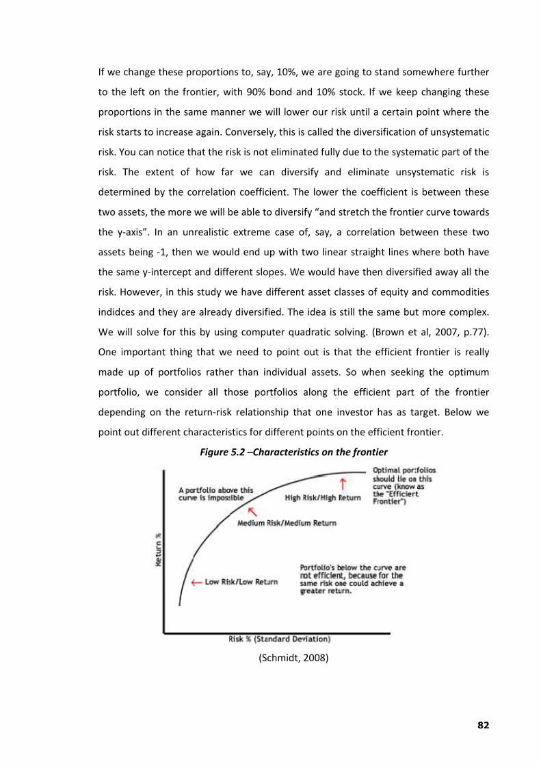
One important thing that we need to point out is that the efficient frontier is really

made up of portfolios rather than individual assets. So when seeking the optimum

portfolio, we consider all those portfolios along the efficient part of the frontier

depending on the return-risk relationship that one investor has as target. Below we

point out different characteristics for different points on the efficient frontier.

Figure 5.2 –Characteristics on the frontier

(Schmidt, 2008)

83

5.2 – ASSUMPTIONS OF MPT MODEL

Markowitz model, as many other models, is based on assumptions that need to be

taken under consideration when dealing with MPT.

1. Investors ask for maximizing the expected return of their total wealth.

2. All investors have the similar expected single period investment horizon.

3. All investors are risk-averse, which means that they only will accept a higher risk

if they are compensated with a higher expected return.

4. Investors base their entire investment decision on the expected return and risk.

5. Investors prefer higher returns to lower returns for a given level of risk.

Based on these assumptions, most of which are pretty much common sense, when

comparing a single asset or a portfolio of assets, only assets or portfolios with the

highest expected return at the same or lower risk level are considered as efficient.

(Francis and Ibbotson, 2002, p.402)

Versijp (2011) adds the following assumptions for modern portfolio theory to our list.

1. Investors prefer more over less (no satiation)

2. Investors dislike risk (risk-aversion)

3. Traders maximize utility, and do so for 1 period

4. Utility is a function of expected return and variance and nothing else

5. There is no distortion from inflation

6. All information is available at no costs

7. All investments are infinitely divisible

And last one which should be on our assumption list for proper analysis

8. The unit of measurement contains a constant purchasing power.

Of course this list is not the best representation of reality, but allows to do

valuable analysis.

Investors are also rational so they will always prefer more to less, i.e. investors will not

invest in a portfolio if there consists a second portfolio with a more favorable risk-

return profile. Security markets are efficient, as new information enter markets

information is quickly reflected in the assets prices. Assets are therefore literally re-

84

priced as soon as new information hit the market. MPT also uses standard deviation

(volatility) as a proxy for risk.

Another assumption of the MPT is that there are no limits on the size of positions taken

when investing and investors can take any position they want. Investors don’t think

about taxes when making investments decisions and are indifferent between receiving

dividends or capital gains. Investors also don’t have to think about transaction costs.

Investors as a group also look at the risk-return relationship over the same time

horizon. All assets, including human capital can be traded on the market and politics

and investor psychology have no effect on the markets. MPT further assumes that

returns are normally distributed and that historical average of returns corresponds to

expected returns.

Objectives and constraints

The main objective is to minimize risk with respect to every level of expected portfolio

returns. This is a matter of a programming problem, since the objective function is in

quadratic form for the weight allocation to each asset.

In this study we will only work with two constraints. Firstly, we put constraint on each

generated (optimal) portfolio’s risk to be minimized. Secondly, the weight, xi, allocation

to each asset cannot be less than 0% (short sales restricted) or more than 100%

(leverage restricted).

To solve this we have used the financial toolbox of Matlab and the function frontcon

where the parameters are,

Inputs

Expected Returns for all assets

Expected covariance matrix

Number of portfolios to generate on the frontier

Constraints on weights

85

Outputs

Vector of efficient expected portfolio returns

Vector of efficient portfolio risks

Matrix of optimal portfolio weights.

Once this is obtained, we can create the efficient frontier by plotting all the returns

versus the risk levels on the mean-variance space. (The MathWorks, 2010) See

Appendix A for a more detailed description and short example for a simple portfolio

using this function.

5.3 - CHARACTERISTICS OF ASSETS

As stated earlier the relationship of risk and return is a key issue in MPT and this

chapter presents the definition of risk and return as individual assets and shows how

risk and return are measured in portfolios. When investor faces risk he can’t expect to

get the same payoff from investment in any asset. The payoff from any investment for

the investor can be described by two main attributes: A measure of central tendency

called the expected return and a measure of risk or dispersion around the mean, called

the standard deviation (Elton et al, 2011, p.44).

The measure of average return is defined as expected return. If Pij is the probability of

the jth return on the ith asset and Rij is the jth return on the ith asset, then the

expected return is a probability weighted average of all outcomes and is calculated as

follows:

��3�� � . =�;3�;1

;2�

Equation – 5.1

The second attribute of the risk-return relationship is the measure of how much

outcomes differ from the average return, i.e. the variance. The variance of the return

on the ith asset is calculated as follows:

86

8�9 � . >=�;?3�; � ��3��@9A1

;2�

Equation – 5.2

This dispersion around the mean is often defined as standard deviation, where the

standard deviation is just the square root of the variance:

86 � B8�9

Equation – 5.3

Standard deviation of expected returns is used as a measure for risk for individual

assets of portfolios. The standard deviation is a measure of volatility in the way that the

more an asset’s return varies from its mean, the more volatile the asset is. The more

the volatility is, the higher the standard deviation is which means that the asset is more

risky.

5.4 – RISK & RETURN CHARACTERISTICS OF PORTFOLIOS

The expected return on a portfolio is calculated as a weighted average of the return on

the individual assets that form the portfolio. It is mathematically expressed as follows:

��34� � . /� ��3��1

�2�

Equation – 5.4

Where E(Rp) is the expected return of a portfolio, Wi is the weight invested in asset i

and E(Ri) is the expected return of asset i.

When calculating the risk or volatility (standard deviation) of portfolio the concept of

covariance becomes significant. Risk on a portfolio is not just a simple average of the

risk on the individual assets forming the portfolio. The risk depends on whether returns

on the individual assets tend to move together, i.e. whether some assets give good

returns when others give bad returns. If assets don’t move together in perfect harmony

87

then there is a risk reduction possibility by holding them together in a portfolio. The

variance of portfolio is calculated as follow:

849 � . /�98� :1

�2�. . /�/;

1

;2�8�8�<�;

1

;2�

Equation – 5.5

Where Wi and Wj are the weights in assets i and j invested in the portfolio and 8�8�<�; is

the covariance between assets i and j. The concept of covariance is further described in

detail.

5.5 - DIVERSIFICATION EFFECT

The investor prefers a stable return during his investment period (Markowitz, 1959;

Sharpe, 1970). This implies that according to the investor, the variability must be

minimal. The investor can minimize this variability by investing in variety of assets.

Holding a variety of assets is also called a portfolio (Bodie, Kane, & Marcus, 2009). Thus,

by forming a portfolio, an investor can create a stable return. However, this process has

its limits. An investor can add one or more assets to his portfolio until the additional

asset does not reduce the variability or when the added benefits becomes less than the

costs of comparison and computation (Bodie, et al., 2009; Sharpe, 1970). This process is

also called diversification.

Covariance and correlation are concepts that are very important measures to discuss to

be able to understand the benefits of diversification. Covariance is a measure of how

returns on assets move together. It is a product of two deviations, i.e. the return of

security X from its mean and the deviation of the returns on security Y from its mean. If

e.g. two assets, X and Y, give both good outcomes at the same time or bad outcomes at

the same time then the covariance will be a positive number. On the other hand, if

security X gives good outcome and security Y gives bad outcome at the same time, the

covariance will be negative. The covariance is calculated as follows:

CDE�� � 8�� � . �3�� � ��3��+F3�� � �?3�@GH

1

�2�

Equation – 5.6

88

Where X and Y are two assets, and E(Rx) and E(Ry)are expected returns on assets X and

Y and n is the number of observations and Rxi and Ryi are the ith return on asset X and

Y. It can be useful to standardize the covariance since it can be difficult to compare

covariance among data sets with different scales (e.g. kilo or pounds). Correlation

coefficient is a standardized version of the covariance where the covariance is divided

between two assets by the product of the standard deviation of each asset. The formula

for the correlation coefficient is as follows:

<�; � CDE��8�8�

Equation – 5.7

This standardization does not change the properties of the covariance it simply scales

the correlation coefficient to have values between the range of -1 to +1. If the

correlation coefficient between X and Y is positive then these two securities tend to

move in the some direction. On the other hand, if the correlation coefficient is negative

they tend to move in the opposite direction.

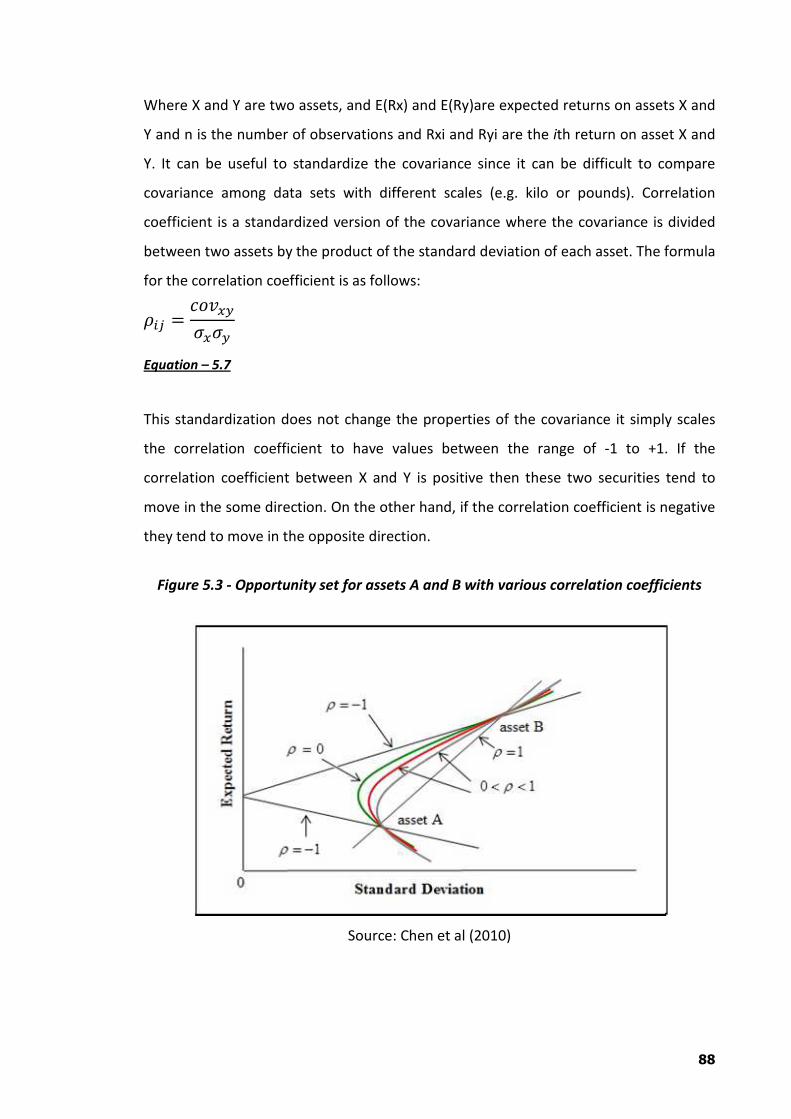
Figure 5.3 - Opportunity set for assets A and B with various correlation coefficients

Source: Chen et al (2010)

89

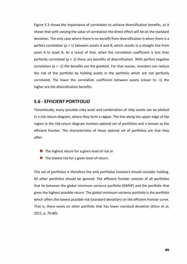
Figure 5.3 shows the importance of correlation to achieve diversification benefits, as it

shows that with varying the value of correlation the direct effect will be on the standard

deviation. The only case where there is no benefit from diversification is when there is a

perfect correlation (ρ = 1) between assets A and B, which results in a straight line from

asset A to asset B. As a result of that, when the correlation coefficient is less than

perfectly correlated (ρ < 1) there are benefits of diversification. With perfect negative

correlation (ρ = -1) the benefits are the greatest. For that reason, investors can reduce

the risk of the portfolio by holding assets in the portfolio which are not perfectly

correlated. The lower the correlation coefficient between assets (closer to -1) the

higher are the diversification benefits.

5.6 - EFFICIENT PORTFOLIO

Theoretically, every possible risky asset and combination of risky assets can be plotted

in a risk-return diagram, where they form a region. The line along the upper edge of the

region in the risk-return diagram involves optimal set of portfolios and is known as the

efficient frontier. The characteristics of these optimal set of portfolios are that they

offer:

The highest return for a given level of risk or

The lowest risk for a given level of return.

This set of portfolios is therefore the only portfolios investors should consider holding.

All other portfolios should be ignored. The efficient frontier consists of all portfolios

that lie between the global minimum variance portfolio (GMVP) and the portfolio that

gives the highest possible return. The global minimum variance portfolio is the portfolio

which offers the lowest possible risk (standard deviation) on the efficient frontier curve.

That is, there exists no other portfolio that has lower standard deviation (Elton et al,

2011, p. 79-80).

90

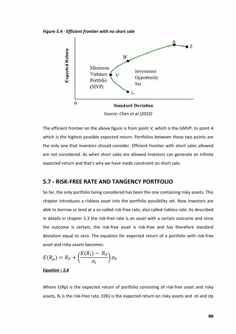
Figure 5.4 - Efficient frontier with no short sale

Source: Chen et al (2010)

The efficient frontier on the above figure is from point V, which is the GMVP, to point A

which is the highest possible expected return. Portfolios between these two points are

the only one that investors should consider. Efficient frontier with short sales allowed

are not considered. As when short sales are allowed investors can generate an infinite

expected return and that’s why we have made constraint on short sale.

5.7 - RISK-FREE RATE AND TANGENCY PORTFOLIO

So far, the only portfolio being considered has been the one containing risky assets. This

chapter introduces a riskless asset into the portfolio possibility set. Now investors are

able to borrow or lend at a so-called risk-free rate, also called riskless rate. As described

in details in chapter 5.3 the risk-free rate is an asset with a certain outcome and since

the outcome is certain, the risk-free asset is risk-free and has therefore standard

deviation equal to zero. The equation for expected return of a portfolio with risk-free

asset and risky assets becomes:

��34� � 3I : J��3�� � 3I8�

K 8#

Equation – 5.8

Where E(Rp) is the expected return of portfolio consisting of risk-free asset and risky

assets, Rf is the risk-free rate, E(Ri) is the expected return on risky assets and σi and σp

91

are the standard deviations of risky assets and the portfolio. Every combination of

riskless lending or borrowing with risky assets form a straight line in risk-return space

where the intercept on the y-axis (expected return) is Rf and the slope of the line is

equal to L)�*$�� *MN$

O and is called the Sharpe ratio. This line is called Capital Market

Line (CML).

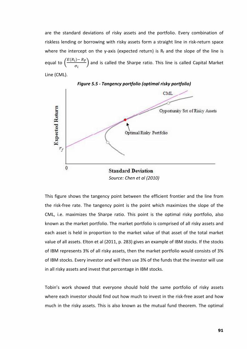
Figure 5.5 - Tangency portfolio (optimal risky portfolio)

Source: Chen et al (2010)

This figure shows the tangency point between the efficient frontier and the line from

the risk-free rate. The tangency point is the point which maximizes the slope of the

CML, i.e. maximizes the Sharpe ratio. This point is the optimal risky portfolio, also

known as the market portfolio. The market portfolio is comprised of all risky assets and

each asset is held in proportion to the market value of that asset of the total market

value of all assets. Elton et al (2011, p. 283) gives an example of IBM stocks. If the stocks

of IBM represents 3% of all risky assets, then the market portfolio would consists of 3%

of IBM stocks. Every investor and will then use 3% of the funds that the investor will use

in all risky assets and invest that percentage in IBM stocks.

Tobin’s work showed that everyone should hold the same portfolio of risky assets

where each investor should find out how much to invest in the risk-free asset and how

much in the risky assets. This is also known as the mutual fund theorem. The optimal

92

portfolio for each investor is dependent on how much the investor is willing to invest in

the risk-free asset and the tangency portfolio.

Every rational investor will hold the tangency portfolio while risk-seeking investors will

borrow at the risk-free rate to invest in the tangency portfolio. Very risk-averse investor

will on the other hand invest part of their funds in the risk-free rate and part of it in the

tangency portfolio. All efficient portfolios will lie along the CML (Elton et al, 2011, p.

283).

5.8 - OPTIMAL PORTFOLIO AND THE INVESTMENT HORIZON

Once we have indentified all efficient portfolios we will now further indentify the most

optimal portfolio from these. This is done by finding the one portfolio that possesses

the highest reward-to-variability, or in other words, the highest Sharpe ratio. To be able

to do this we are now going to introduce the riskless asset into the mean variance

space.

The investor wants a stable return during his investment period, so his goal is to form a

portfolio that gives the most stable and desired expected return during his investment

period. The portfolio that gives the desired expected return with the lowest variability

will be defined as the optimal portfolio (Markowitz 1952).

Once this particular portfolio is found we will denote it the Optimal Risky Portfolio. This

portfolio is the one portfolio that would be suggested to an investor with unknown risk

preference, since it is judged to yield a moderate risk aversion coefficient level. (Brown

et al, 2007, p.104-105). At this point we are now standing with two alternatives

investments, the riskless asset and the Optimal risky portfolio. The question now is

what investment horizon of combination is there between these two assets? The way

to solve for this is basically the same as we did before, that is to find the efficient

frontier by the MVO method. But now we are incorporating a risky free asset in our

risky portfolio. Since we are only dealing with two assets the whole objective is a lot

easier. The riskless asset becomes the y-intercept and the Sharpe ratio the slope of this

93

linear equation. This equation is our investment horizon (or also efficient frontier) and

is called the Capital Allocation Line.

PQR � 3S : JRT � RU σT

K σ

Equation – 5.9

We can now understand from this equation that that we can either invest some or all of

our investments to the riskless asset (lend money to, in our case, the government) or

invest 100% or more (leverage the Sharpe portfolio) in the Sharpe portfolio. Recall that

if the Sharpe portfolio’s return replicates the market’s return, it is then called the

market portfolio and the CAL will then be called the Capital Market line. Also, if one

chooses to buy (that is to replicate) the market portfolio, then he or she is having a

passive portfolio strategy. (Bodie, Kane, Marcus, Perrakis, and Ryan, 2008, p.184)

The investor can construct multiple efficient portfolios. However, the investor is only

interested in the portfolio that gives the expected return that he prefers but with the

lowest variability. So the investor has already predetermined the expected return

before the portfolio has been constructed. Thus the optimal portfolio will be defined as

the portfolio that gives the expected return that is predetermined by the investor but

with the lowest variability and will be located at the capital allocation line (CAL). The

optimal portfolio differs for each investor but the goal for each investor is the same:

find his optimal portfolio.

Current literature has either used data before the crisis in 2008 or has looked at the

efficient frontier. The efficient frontier is a collection of efficient portfolios. An efficient

portfolio will be defined as a portfolio that cannot obtain a greater average return

without incurring greater risk or when it is impossible to reduce risk without sacrificing

its return (Markowitz, 1959).

5.9 - UTILITY AND RISK AVERSION

Now the point is reached where the need to establish an optimal weight allocation

between riskless asset and the Sharpe portfolio, tailored for a reasonable investor. It

will of course be difficult for an asset manager to give his client the exactly correct

94

portfolio combination without knowing his preferences. So what many financial

theorists do is that they quantify the investors risk preference with respect to risk. The

obtained quantity is denoted by the letter A, also called the Risk aversion coefficient. It

is a matter of questioning the client and issue surveys and is a big matter in behavioral

finance. The more risk avert an investor is, the more he or she will consider risk free

investments, since there is less uncertainty with this strategy. But on the other hand, if

one is less risk avert, he or she will accept higher risk with sufficiently higher expected

return compensation, in other words, a higher risk premium for each additional risk

level. (Bodie et al, 2008, p.173).

The discussion will now move further into how to use this risk aversion amount in order

to be able to identify the optimal portfolio in the mean-variance-space. To do so, utility

functions have been introduced, which is a way to assign a number to every possible

asset combination such that more preferred asset combinations get assigned higher

numbers than less-preferred. (Varian, 2008)

A very common utility function that is widely used by financial economists is

W � ��X� � 0.005 \ Q \ 89

Equation – 5.10

Where –

U is the utility value

E(r) is the expected return

A is the index of investor's aversion

σ is the standard deviation

Firstly, by making observations to this model, one can begin to notice that the higher

the risk aversion value, A, gets, the more it will penalize the whole utility score when

subtracting away the amount 0.005* A* *σ2 Secondly, one can observe that a higher

expected return will contribute with a higher utility score, while simultaneously the

higher risk level will lower it. Thirdly, if one would have only invested in a riskless asset

he or she would yield a utility score equal to the expected return since the risk is equal

95

to zero, making the last term vanish. So this specific utility function makes perfect

sense. (The factor of 1⁄2 (0.005) is a scaling convention that will simplify calculations in

later. It has no economic significance, and we could eliminate it simply by defining a

“new” A with half the value of the A used here)

The next step is to build an indifference curve that represents a fixed utility. The

indifference curves are constructed by simply solving for E(R) and fix the utility score

and the risk aversion and then put increments on the risk.

One will find several expected returns by each increment of risk, and at the same time

maintain the same level of utility. An example of this is illustrated below.

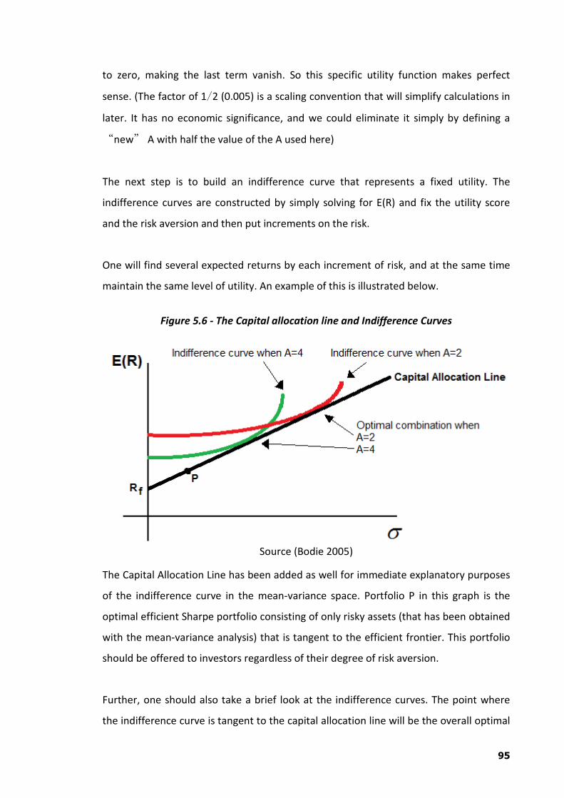
Figure 5.6 - The Capital allocation line and Indifference Curves

Source (Bodie 2005)

The Capital Allocation Line has been added as well for immediate explanatory purposes

of the indifference curve in the mean-variance space. Portfolio P in this graph is the

optimal efficient Sharpe portfolio consisting of only risky assets (that has been obtained

with the mean-variance analysis) that is tangent to the efficient frontier. This portfolio

should be offered to investors regardless of their degree of risk aversion.

Further, one should also take a brief look at the indifference curves. The point where

the indifference curve is tangent to the capital allocation line will be the overall optimal

96

portfolio for investors given risk aversion. This portfolio is also called The Complete

Portfolio. It should be emphasized that the indifference curve could end up below the

Sharpe portfolio on the CAL with a significantly high risk aversion. In general, if one was

risk-neutral, the indifference curve would rather be a straight line, and with a risk-loving

attitude the curve is instead convex somewhere below the efficient frontier (Bodie et al,

2008. P187-192)

5.10 - THE COMPLETE PORTFOLIO DERIVATION (ALLOCATION

BETWEEN THE RISKLESS AND THE RISKY ASSET)

So far the overall optimal portfolio has graphically been pointed out where it lies on the

mean-variance space, but what is the specific asset combination at that point? Let’s

start over from the beginning. So far the capital allocation line has been calculated

which represents an investment opportunity set of combination of one riskless asset

and one portfolio of risky assets (the optimal Sharpe portfolio). It is now important to

decide what combination of the riskless asset and the risky Sharpe portfolio should be.

What exact combination will give the highest utility? It will of course be the one where

we have a maximized utility. So let’s do that.

First let y denote the weight put in risky portfolio. Then one can form the equations for

the complete portfolio, C.

E�R^� : ��?R_@ : �1 � �� ��RU� � RU : yFE?R_@ � RUG

Equation – 5.11

Where, one can see that he or she has risk premium in the last term for each additional

weight allocation in y. One can further denote the risk to be

8a � �84

Equation – 5.12

Solve for y and get that

� � -b-c

Equation – 5.13

97

Now substitute y into the first equation and obtain

��3a� � 3S : 8aFE?R_@ � RU�G

σT

Equation – 5.14

This defines the Capital Allocation line in the mean-variance space. Notice that the

slope is the Sharpe ratio (risk premium divided by the risk of risky portfolio (or, market

portfolio).

Now all the components needed exist in order to be able to maximize the utility

function for the complete portfolio with respect to y.

Now solve for y and get that

�d4!�efg � E�RT� � RU0.01AσT9

Equation – 5.15

This weight will be the optimal choice of investment in the risky portfolio according to a

given risk aversion preference. Notice that if the risk aversion coefficient gets very large

in the denominator, the whole expression will get closer to zero, meaning that the more

risk averts an investor is, the less weight, y, he or she would put in the risky asset.

5.11 - CRITICISM OF MPT

Modern portfolio theory has received some criticism throughout the years because of

the assumptions behind the model of MPT which some academics and investors find

unrealistic. Some have questioned MPT’s definition of risk and questions are raised

whether volatility, measured as variance or standard deviation is a good measure for

risk. It has been pointed out that the assumption of variance being constant over time

isn’t always true. The option market is a good example, where option traders do not

quote the same volatility every day (Morien, 2011). Some have pointed out that there

aren’t any permanent correlations between risk and reward, i.e. high volatility does not

give better rewards and low volatility does not give lesser rewards. Murphy (1997)

98

concluded in his study that the realized return seemed to be higher than expected for

low risk securities. According to Murphy’s results, a conclusion can be drawn that the

relationship between risk and reward is weaker than expected. Haugen & Heins (1975)

also found out in their study that risk does not generate a special reward.

The liquidity assumption in MPT has been criticized and the recent 2008 financial crisis

has proved that some markets can be illiquid. MPT has also been criticized for not

having much similarity to real life situations since the theory assumes that there are no

transaction cost and no taxes. Investors in real life do face some transaction cost when

investing which has impact on short versus long term investments. Real life investors

also pay taxes (in most cases) on their investments income which has effect on what

kind of investments are chosen. The assumption of short sales being allowed is

questionable since short selling is illegal or restricted in some countries (Morien, 2011).

It has also been pointed out that there is really no such thing as a risk-free rate available

to investors. Finally, investors often do not behave rationally and follow rumors, hot

stocks or glamorous stocks. Investors even get overconfident and make irrational

decisions.

Also Markowitz (1959) measures variability by using standard deviation, so Markowitz

assumes that returns of assets are normally distributed. This assumption is not realistic

because history has shown otherwise (Michaud & Michaud, 2008; Tarasi, Bolton, Hutt,

& Walker, 2011). For example equity is not symmetrically distributed but has a negative

skewness (Gorton & Rouwenhorst, 2006; Michaud & Michaud, 2008). As result,

investors are using the variability and the expected return of assets to form the optimal

portfolio.

The input to find/construct the optimal portfolio is essential, Markowitz used ex post

return and variance to determine the optimal portfolio. However some researchers

raise question with respect to that as well. But in totality if we see than, keeping aside

the criticism, MPT model is one of the most widely used model for strategic asset

allocation studies.