4421 chapter 12_-_discrete_fourier_transform (2)

P1: RPU/XXX P2: RPU/XXX QC: RPU/XXX T1: RPU

CUUK852-Mandal & Asif November 17, 2006 15:45

C H A P T E R

12 Discrete Fourier transform

In Chapter 11, we introduced the discrete-time Fourier transform (DTFT) thatprovides us with alternative representations for DT sequences. The DTFT trans-forms a DT sequence x[k] into a function X () in the DTFT frequency domain. The independent variable is continuous and is confined to the range – ≤ < . With the increased use of digital computers and specialized hard-ware in signal processing, interest has focused around transforms that are suit-able for digital computations. Because of the continuous nature of , directimplementation of the DTFT is not suitable on such digital devices. This chapterintroduces the discrete Fourier transform (DFT), which can be computed effi-ciently on digital computers and other digital signal processing (DSP) boards.

The DFT is an extension of the DTFT for time-limited sequences with anadditional restriction that the frequency is discretized to a finite set of valuesgiven by = 2r/M , for 0 ≤ r ≤ (M − 1). The number M of the frequencysamples can have any value, but is typically set equal to the length N of the time-limited sequence x[k]. If M is chosen to be a power of 2, then it is possible toderive extremely efficient implementations of the DFT. These implementationsare collectively referred to as the fast Fourier transform (FFT) and, for anM-point DFT, have a computational complexity of O(M log2 M). This chapterdiscusses a popular FFT implementation and extends the theoretical DTFTresults derived in Chapter 11 to the DFT.

The organization of this chapter is as follows. Section 12.1 motivates thediscussion of the DFT by expressing it as a special case of the continuous-timeFourier transform (CTFT). The formal definition of the DFT is presented inSection 12.2, including its matrix-vector representation. Section 12.3 applies theDFT to estimation of the spectra of both DT and CT signals. Section 12.4 derivesimportant properties of the DFT, while Section 12.5 uses the DFT as a tool toconvolve two DT sequences in the frequency domain. A fast implementation ofthe DFT based on the decimation-in-time algorithm is presented in Section 12.6.Finally, Section 12.7 concludes the chapter with a summary of the importantconcepts.

525



526 Part III Discrete-time signals and systems

12.1 Continuous to discrete Fourier transform

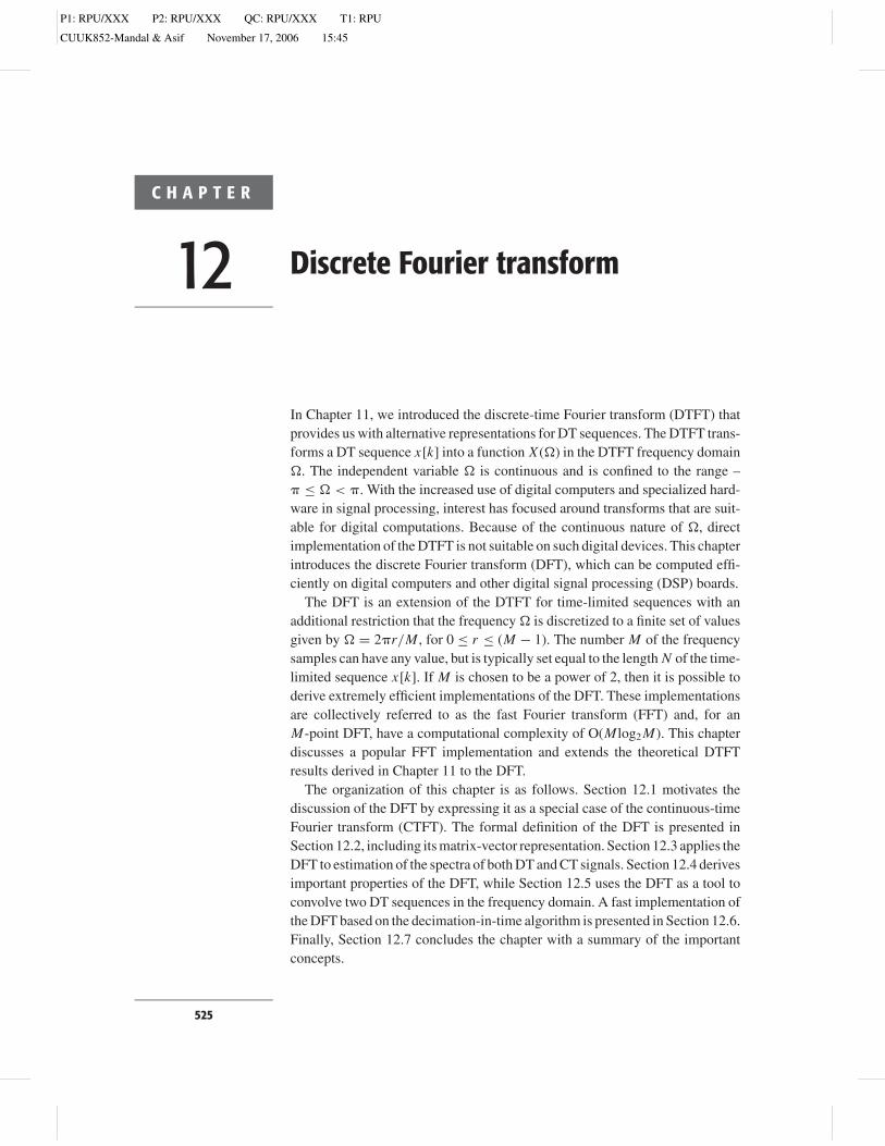
In order to motivate the discussion of the DFT, let us assume that we areinterested in computing the CTFT of a CT signal x(t) using a digital computer.The three main steps involved in the computation of the CTFT are illustrated inFig. 12.1. The waveforms for the CT signal x(t) and its CTFT X (), shown inFigs 12.1(a) and (b), are arbitrarily chosen, so the following procedure appliesto any CT signal. A brief explanation of each of the three steps is providedbelow.

Step 1: Analog-to-digital conversion In order to store a CT signal into adigital computer, the CT signal is digitized. This is achieved through two pro-cesses known as sampling and quantization, collectively referred to as analog-to-digital (A/D) conversion by convention. In this discussion, we only considersampling, ignoring the distortion introduced by quantization. The CT signalx(t) is sampled by multiplying it by an impulse train:

s1(t) =∞∑

m=−∞(t − mT1), (12.1)

illustrated in Fig. 12.1(c). The sampled waveform is given by x1(t) = x(t)s1(t),which is shown in Fig. 12.1(e). Since multiplication in the time domain isequivalent to convolution in the frequency domain, the CTFT X1() of thesampled signal x1(t) is given by the following transform pair:

x1(t) = x(t) ×∞∑

m=−∞(t − mT1)

CTFT←→ X1()

= 1

2

[X () ∗ 2

T1

∞∑m=−∞

(

− 2m

T1

)](12.2)

or

x1(t) =∞∑

m=−∞x(mT1)(t − mT1)

CTFT←→ X1() = 1

T1

∞∑m=−∞

X(

− 2m

T1

).

(12.3)

The above result is derived in Eq. (9.5) of Chapter 9 and is graphically illustratedin Figs 12.1(b), (d), and (f), where we note that the spacing between adjacentreplicas of X () in X1() is given by 2/T1. Since no restriction is imposedon the bandwidth of the CT signal x(t), limited aliasing may also be introducedin X1().

To derive the discretized representation of x(t) from Eq. (12.3), sampling isfollowed by an additional step (shown in Fig. 12.1(g)), where the CT impulsesare converted to the DT impulses. Equation (12.3) can now be extended to



527 12 Discrete Fourier transform

ω0

X(ω)1

k0

x1[k]A

1 2 3

x1(t)

t0

A

T1

0t

x(t)A

t

s1(t)

1

T10ω

S1(ω)

X1(ω)

X1(Ω)

2πT1

1T1

1T1

04πT1

−

4πT1

− 2πT1

− 2πT1

4πT1

2πT1

− 2πT1

4πT1

ω0

Ω0 2π 4π−2π−4π

w[k]

k

1

0 1 2 … N−1

W(Ω)

Ω

N

0 2π 4π−2π−4π

(a)

(c)

(e)

(d)

(f)

(g) (h)

(i) (j)

(b)

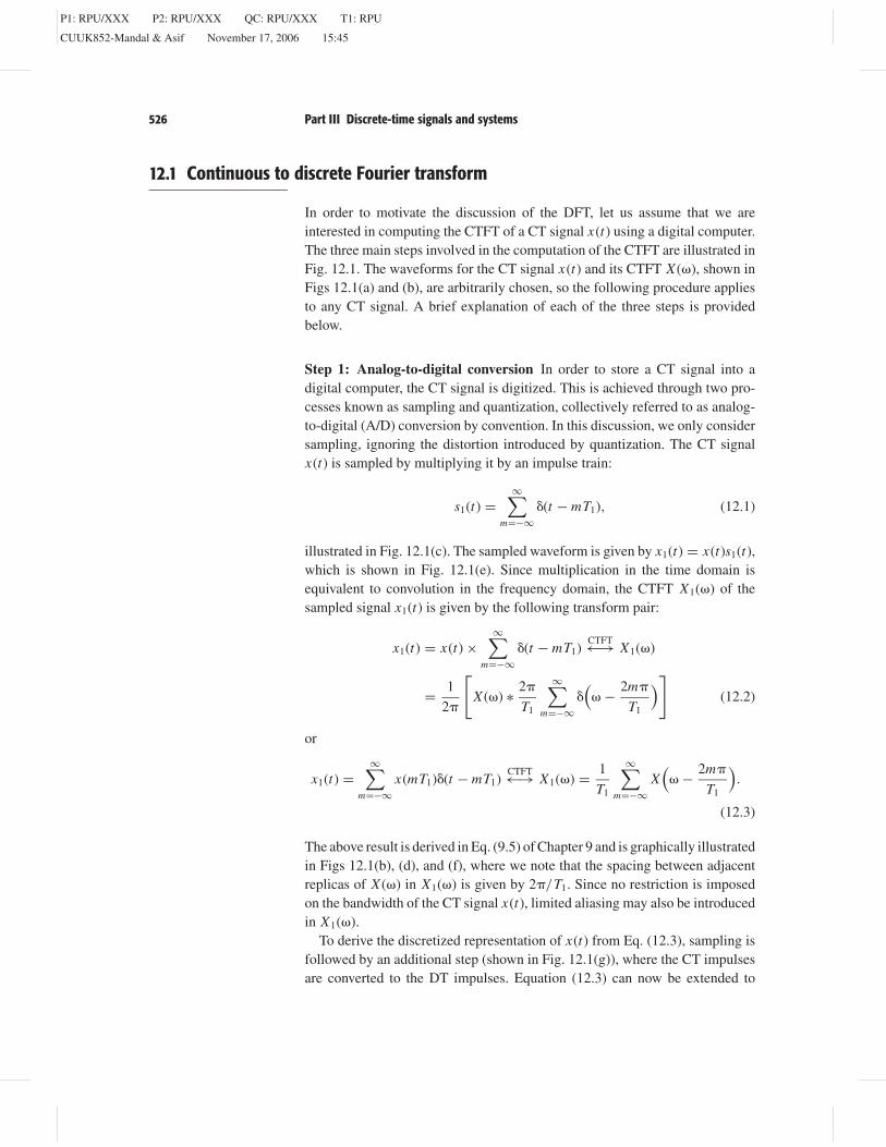
Fig. 12.1. Graphical derivation of the discrete Fourier transform pair.Original CT signal. (b) CTFT of the original CT signal. (c) Impulse trainsampling of CT signal. (d) CTFT of the impulse train in part (c). (e) CTsampled signal. (f) CTFT of the sampled signal in part (e). (g) DTrepresentation of CT signal in part (a). (h) DTFT of the DTrepresentation in part (g). (i) Rectangular windowing sequence.(j) DTFT of the rectangular window. (k) Time-limited sequencerepresenting part (g). (1) DTFT of time-limited sequence in part(k). (m) Inverse DTFT of frequency-domain impulse train in part (n).(n) Frequency-domain impulse train.




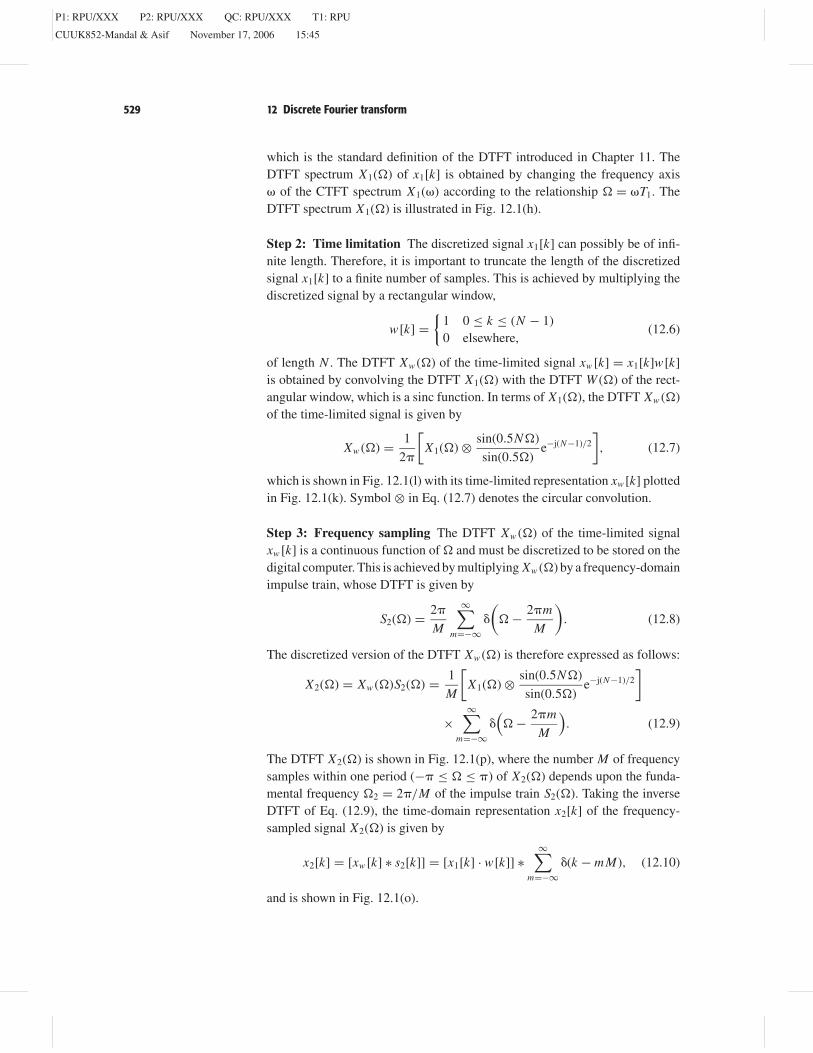
Xw(Ω)

k

xw[k]A

0 1 2 … N−1 −4π −2π 2πΩ

2πT1

N

0 4π

s2[k]

0k

1

M−M

x2[k]

0k

A

0 1 2 … N−1 M

00 1 2 … N−1 M

S2(Ω)

Ω

M2π

0 2π 4π−2π−4π

−M

−M

M2π

Xw(Ω)

Ω

MT1

N

0 2π 4π−2π−4πM2π

X2[r]

r

0 M 2M−M−2M

MT1

Nx2[k]

k

A

(k) (l)

(m) (n)

(o) (p)

(q) (r)

Fig. 12.1. (cont.) derive the DTFT of the DT sequence x1[k] as follows:

x1[k] =∞∑

m=−∞x(mT1)(t − mT1). (12.4)

Taking the DTFT of both sides of Eq. (12.4) yields

X1() =∞∑

m=−∞x(mT1)e−jmT1 . (12.5)

Substituting x1[m] = x(mT 1) and = T1 in Eq. (12.5) leads to

X1() = X1()|=/T1 =∞∑

m=−∞x1[m]e−jm,




which is the standard definition of the DTFT introduced in Chapter 11. TheDTFT spectrum X1() of x1[k] is obtained by changing the frequency axis of the CTFT spectrum X1() according to the relationship = T1. TheDTFT spectrum X1() is illustrated in Fig. 12.1(h).

Step 2: Time limitation The discretized signal x1[k] can possibly be of infi-nite length. Therefore, it is important to truncate the length of the discretizedsignal x1[k] to a finite number of samples. This is achieved by multiplying thediscretized signal by a rectangular window,

w[k] =

1 0 ≤ k ≤ (N − 1)0 elsewhere,

(12.6)

of length N . The DTFT Xw () of the time-limited signal xw [k] = x1[k]w[k]is obtained by convolving the DTFT X1() with the DTFT W () of the rect-angular window, which is a sinc function. In terms of X1(), the DTFT Xw ()of the time-limited signal is given by

Xw () = 1

2

[X1() ⊗ sin(0.5N)

sin(0.5)e−j(N−1)/2

], (12.7)

which is shown in Fig. 12.1(l) with its time-limited representation xw [k] plottedin Fig. 12.1(k). Symbol ⊗ in Eq. (12.7) denotes the circular convolution.

Step 3: Frequency sampling The DTFT Xw () of the time-limited signalxw [k] is a continuous function of and must be discretized to be stored on thedigital computer. This is achieved by multiplying Xw () by a frequency-domainimpulse train, whose DTFT is given by

S2() = 2

M

∞∑m=−∞

( − 2m

M

). (12.8)

The discretized version of the DTFT Xw () is therefore expressed as follows:

X2() = Xw ()S2() = 1

M

[X1() ⊗ sin(0.5N)

sin(0.5)e−j(N−1)/2

]

×∞∑

m=−∞( − 2m

M

). (12.9)

The DTFT X2() is shown in Fig. 12.1(p), where the number M of frequencysamples within one period (− ≤ ≤ ) of X2() depends upon the funda-mental frequency 2 = 2/M of the impulse train S2(). Taking the inverseDTFT of Eq. (12.9), the time-domain representation x2[k] of the frequency-sampled signal X2() is given by

x2[k] = [xw [k] ∗ s2[k]] = [x1[k] · w[k]] ∗∞∑

m=−∞(k − mM), (12.10)

and is shown in Fig. 12.1(o).




The discretized version of the DTFT Xw () is referred to as the discreteFourier transform (DFT) and is generally represented as a function of the fre-quency index r corresponding to DTFT frequency r = 2r/M , for 0 ≤ r ≤(M− 1). To derive the expression for the DFT, we substitute = 2r/M inthe following definition of the DTFT:

X2() =N−1∑k=0

x2[k]e−jk, (12.11)

where we have assumed x2[k] to be a time-limited sequence of length N .Equation (12.11) reduces as follows:

X2(r ) =N−1∑k=0

x2[k]e−j(2kr/M), (12.12)

for 0 ≤ r ≤ (M−1). Equation (12.12) defines the discrete Fourier transform(DFT) and can easily be implemented on a digital device since it converts adiscrete number N of input samples in x2[k] to a discrete number M of DFTsamples in X2(r ). To illustrate the discrete nature of the DFT, the DFT X2(r )is also denoted asX2[r ]. The DFT spectrum X2[r ] is plotted in Fig. 12.1(r).

Let us now return to the original problem of determining the CTFT X ()of the original CT signal x(t) on a digital device. Given X2[r ] = X2(r ), itis straightforward to derive the CTFT X () of the original CT signal x(t) bycomparing the CTFT spectrum, shown in Fig. 12.1(b), with the DFT spectrum,shown in Fig. 12.1(r). We note that one period of the DFT spectrum within therange −0.5(M−1) ≤ r ≤ 0.5(M−1) (assuming M to be odd) is a fairly goodapproximation of the CTFT spectrum. This observation leads to the followingrelationship:

X (r ) ≈ MT1

NX2[r ] = MT1

N

N−1∑k=0

x2[k]e−j(2kr/M), (12.13)

where the CT frequencies r = r/T1 = 2r/(M × T1) for −0.5(M − 1) ≤r ≤ 0.5(M−1).

Although Fig. 12.1 illustrates the validity of Eq. (12.1) by showing that theCTFT X () and the DFT X2[r ] are similar, there are slight variations in the twospectra. These variations result from aliasing in Step 1 and loss of samples inStep 2. If the CT signal x(t) is sampled at a sampling rate less than the Nyquistlimit, aliasing between adjacent replicas distorts the signal. A second distortionis introduced when the sampled sequence x1[k] is multiplied by the rectangularwindow w[k] to limit its length to N samples. Some samples of x1[k] are lost inthe process. To eliminate aliasing, the CT signal x(t) should be band-limited,whereas elimination of the time-limited distortion requires x(t) to be of finitelength. These are contradictory requirements since a CT signal cannot be bothtime-limited and band-limited at the same time. As a result, at least one of the




aforementioned distortions would always be present when approximating theCTFT with the DFT. This implies that Eq. (12.12) is an approximation for theCTFT X () that, even at its best, only leads to a near-optimal estimation of thespectral content of the CT signal.

On the other hand, the DFT representation provides an accurate estimate ofthe DTFT of a time-limited sequence x[k] of length N . By comparing the DFTspectrum, Fig. 12.1(h), with the DFT spectrum, Fig. 12.1(r), the relationshipbetween the DTFT X2() and the DFT X2[r ] is derived. Except for a factor ofK/M , we note that X2[r ] provides samples of the DTFT at discrete frequenciesr = 2r/M , for 0 ≤ r ≤ (M−1). The relationship between the DTFT andDFT is therefore given by

X2(r ) = N

MX2[r ] = N

M

N−1∑k=0

x2[k]e−j(2kr/M) (12.14)

for r = 2r/M , for 0 ≤ r ≤ (M−1). We now proceed with the formal defi-nitions for the DFT.

12.2 Discrete Fourier transform

Based on our discussion in Section 12.1, the M-point DFT and inverse DFTfor a time-limited sequence x[k], which is non-zero within the limits 0 ≤ k ≤(N−1), is given by

DFT synthesis equation x[k] = 1

M

M−1∑r=0

X [r ]e j(2kr/M)

for 0 ≤ k ≤ (N − 1); (12.15)

DFT analysis equation X [r ] =N−1∑k=0

x[k]e−j(2kr/M)

for 0 ≤ r ≤ (M − 1). (12.16)

Equation (12.16) was derived in Section 12.1. By substituting the expres-sion for x[k] from the synthesis equation, Eq. (12.15), the analysis equation,Eq. (12.16), can be formally proved. The formal proofs of the DFT pair are leftas an exercise for the reader in Problem 12.1. In Eqs (12.15) and (12.16), thelength M of the DFT is typically set to be greater or equal to the length N ofthe aperiodic sequence x[k]. Unless otherwise stated, we assume M = N in thediscussion that follows. Collectively, the DFT pair is denoted as

x[k]DFT←−−→ X [r ]. (12.17)

Examples 12.1 and 12.2 illustrate the steps involved in calculating the DFTs ofaperiodic sequences.




0 1 2

−1

0

1

2

3

k0 1 2

0

1

2

3

4

5

r0 1 2

−0.5π

−π

0

0.5π

π

r

3 3 3

(a) (b) (c)

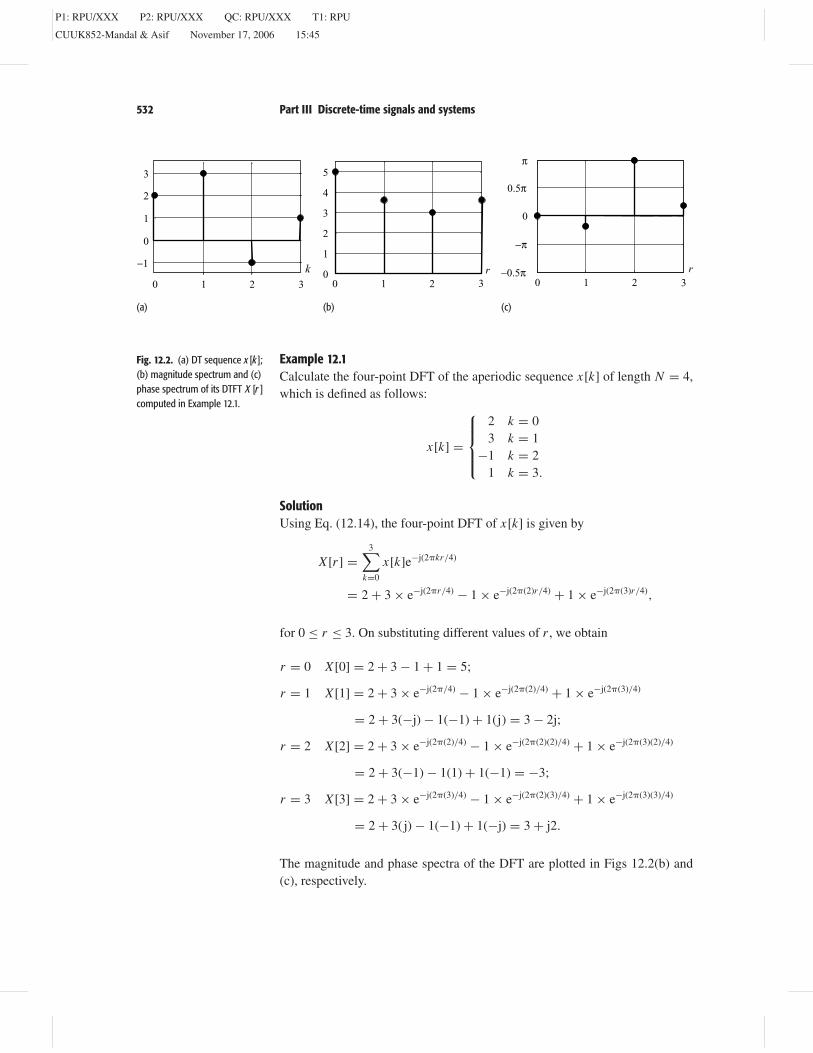
Fig. 12.2. (a) DT sequence x [k ];(b) magnitude spectrum and (c)phase spectrum of its DTFT X [r ]computed in Example 12.1.

Example 12.1Calculate the four-point DFT of the aperiodic sequence x[k] of length N = 4,which is defined as follows:

x[k] =

2 k = 03 k = 1

−1 k = 21 k = 3.

SolutionUsing Eq. (12.14), the four-point DFT of x[k] is given by

X [r ] =3∑

k=0

x[k]e−j(2kr/4)

= 2 + 3 × e−j(2r/4) − 1 × e−j(2(2)r/4) + 1 × e−j(2(3)r/4),

for 0 ≤ r ≤ 3. On substituting different values of r , we obtain

r = 0 X [0] = 2 + 3 − 1 + 1 = 5;

r = 1 X [1] = 2 + 3 × e−j(2/4) − 1 × e−j(2(2)/4) + 1 × e−j(2(3)/4)

= 2 + 3(−j) − 1(−1) + 1(j) = 3 − 2j;

r = 2 X [2] = 2 + 3 × e−j(2(2)/4) − 1 × e−j(2(2)(2)/4) + 1 × e−j(2(3)(2)/4)

= 2 + 3(−1) − 1(1) + 1(−1) = −3;

r = 3 X [3] = 2 + 3 × e−j(2(3)/4) − 1 × e−j(2(2)(3)/4) + 1 × e−j(2(3)(3)/4)

= 2 + 3(j) − 1(−1) + 1(−j) = 3 + j2.

The magnitude and phase spectra of the DFT are plotted in Figs 12.2(b) and(c), respectively.




Example 12.2Calculate the inverse DFT of

X [r ] =

5 r = 03 − j2 r = 1−3 r = 23 + j2 r = 3.

SolutionUsing Eq. (12.13), the inverse DFT of X [r ] is given by

x[k] = 1

4

3∑k=0

X [r ]e j(2kr/4) = 1

4

[5 + (3 − j2) × e j(2k/4) − 3 × e j(2(2)k/4)

+ (3 + j2) × e j(2(3)k/4)],

for 0 ≤ k ≤ 3. On substituting different values of k, we obtain

x[0] = 1

4[5 + (3 − j2) − 3 + (3 + j2)] = 2;

x[1] = 1

4

[5 + (3 − j2)e j(2/4) − 3e j(2(2)/4) + (3 + j2)e j(2(3)/4)

]= 1

4[5 + (3 − j2)( j) − 3(−1) + (3 + j2)(−j)] = 3;

x[2] = 1

4

[5 + (3 − j2)e j(2(2)/4) − 3e j(2(2)(2)/4) + (3 + j2)e j(2(3)(2)/4)

]= 1

4[5 + (3 − j2)(−1) − 3(1) + (3 + j2)(−1)] = −1;

x[3] = 1

4

[5 + (3 − j2)e j(2(3)/4) − 3e j(2(2)(3)/4) + (3 + j2)e j(2(3)(3)/4)

]= 1

4[5 + (3 − j2)(−j) − 3(−1) + (3 + j2)( j)] = 1.

Examples 12.1 and 12.2 prove the following DFT pair:

x[k] =

2 k = 03 k = 1

−1 k = 21 k = 3

DFT←−−→ X [r ] =

5 r = 03 − j2 r = 1−3 r = 23 + j2 r = 3,

where both the DT sequence x[k] and its DFT X [r ] are aperiodic with lengthN = 4.

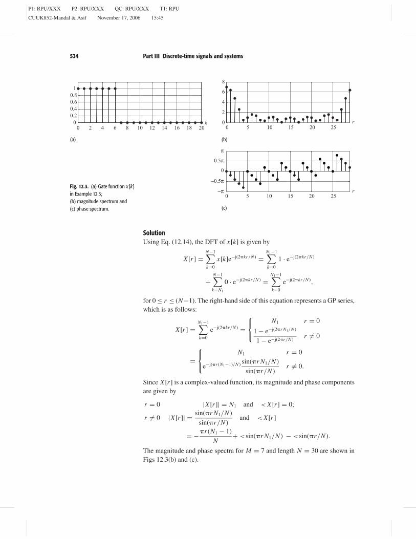
Example 12.3Calculate the N -point DFT of the aperiodic sequence x[k] of length N , whichis defined as follows:

x[k] =

1 0 ≤ k ≤ (N1 − 1)0 N1 ≤ k ≤ N .




0 2 4 6 8 10 12 14 16 18 200

0.20.40.60.8

1

k

0 5 10 15 20 25−π

−0.5π

0

0.5π

π

r

0 5 10 15 20 250

2

4

6

8

r

(a) (b)

(c)

Fig. 12.3. (a) Gate function x [k ]in Example 12.3;(b) magnitude spectrum and(c) phase spectrum.

SolutionUsing Eq. (12.14), the DFT of x[k] is given by

X [r ] =N−1∑k=0

x[k]e−j(2kr/N ) =N1−1∑k=0

1 · e−j(2kr/N )

+N−1∑k=N1

0 · e−j(2kr/N ) =N1−1∑k=0

e−j(2kr/N ),

for 0 ≤ r ≤ (N−1). The right-hand side of this equation represents a GP series,which is as follows:

X [r ] =N1−1∑k=0

e−j(2kr/N ) =

N1 r = 0

1 − e−j(2r N1/N )

1 − e−j(2r/N )r = 0

=

N1 r = 0

e−j(r (N1−1)/N ) sin(r N1/N )

sin(r/N )r = 0.

Since X [r ] is a complex-valued function, its magnitude and phase componentsare given by

r = 0 |X [r ]| = N1 and < X [r ] = 0;

r = 0 |X [r ]| = sin(r N1/N )

sin(r/N )and < X [r ]

= −r (N1 − 1)

N+ <sin(r N1/N ) − <sin(r/N ).

The magnitude and phase spectra for M = 7 and length N = 30 are shown inFigs 12.3(b) and (c).




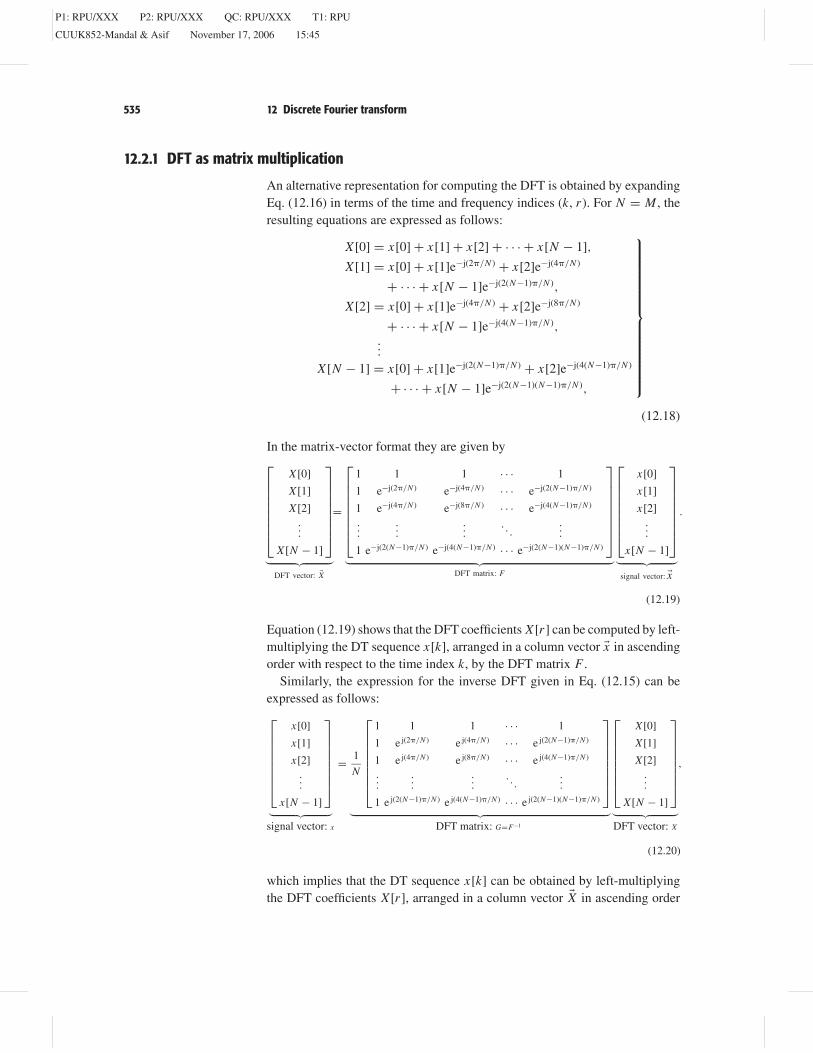
12.2.1 DFT as matrix multiplication

An alternative representation for computing the DFT is obtained by expandingEq. (12.16) in terms of the time and frequency indices (k, r ). For N = M , theresulting equations are expressed as follows:

X [0] = x[0] + x[1] + x[2] + · · · + x[N − 1],

X [1] = x[0] + x[1]e−j(2/N ) + x[2]e−j(4/N )

+ · · · + x[N − 1]e−j(2(N−1)/N ),

X [2] = x[0] + x[1]e−j(4/N ) + x[2]e−j(8/N )

+ · · · + x[N − 1]e−j(4(N−1)/N ),...

X [N − 1] = x[0] + x[1]e−j(2(N−1)/N ) + x[2]e−j(4(N−1)/N )

+ · · · + x[N − 1]e−j(2(N−1)(N−1)/N ),

(12.18)

In the matrix-vector format they are given by

X [0]

X [1]

X [2]...

X [N − 1]

︸︷︷︸DFT vector: X

=

1 1 1 · · · 1

1 e−j(2/N ) e−j(4/N ) · · · e−j(2(N−1)/N )

1 e−j(4/N ) e−j(8/N ) · · · e−j(4(N−1)/N )

......

.... . .

...

1 e−j(2(N−1)/N ) e−j(4(N−1)/N ) · · · e−j(2(N−1)(N−1)/N )

︸︷︷︸DFT matrix: F

x[0]

x[1]

x[2]...

x[N − 1]

︸︷︷︸signal vector: x

.

(12.19)

Equation (12.19) shows that the DFT coefficients X [r ] can be computed by left-multiplying the DT sequence x[k], arranged in a column vector x in ascendingorder with respect to the time index k, by the DFT matrix F .

Similarly, the expression for the inverse DFT given in Eq. (12.15) can beexpressed as follows:

x[0]

x[1]

x[2]...

x[N − 1]

︸︷︷︸signal vector: x

= 1

N

1 1 1 · · · 1

1 e j(2/N ) e j(4/N ) · · · e j(2(N−1)/N )

1 e j(4/N ) e j(8/N ) · · · e j(4(N−1)/N )

......

.... . .

...

1 e j(2(N−1)/N ) e j(4(N−1)/N ) · · · e j(2(N−1)(N−1)/N )

︸︷︷︸DFT matrix: G=F−1

X [0]

X [1]

X [2]...

X [N − 1]

︸︷︷︸DFT vector: X

,

(12.20)

which implies that the DT sequence x[k] can be obtained by left-multiplyingthe DFT coefficients X [r ], arranged in a column vector X in ascending order




with respect to the DFT coefficient index r , by the inverse DFT matrix Gand then scaling the result by a factor 1/N . It is straightforward to show thatG × F = F × G = N IN , where IN is the identity matrix of order N .

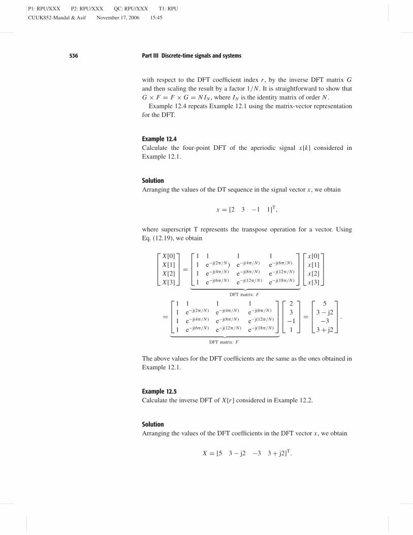
Example 12.4 repeats Example 12.1 using the matrix-vector representationfor the DFT.

Example 12.4Calculate the four-point DFT of the aperiodic signal x[k] considered inExample 12.1.

SolutionArranging the values of the DT sequence in the signal vector x , we obtain

x = [2 3 −1 1]T,

where superscript T represents the transpose operation for a vector. UsingEq. (12.19), we obtain

X [0]X [1]X [2]X [3]

=

1 1 1 11 e−j(2/N ) e−j(4/N ) e−j(6/N )

1 e−j(4/N ) e−j(8/N ) e−j(12/N )

1 e−j(6/N ) e−j(12/N ) e−j(18/N )


x[0]x[1]x[2]x[3]

=

1 1 1 11 e−j(2/N ) e−j(4/N ) e−j(6/N )

1 e−j(4/N ) e−j(8/N ) e−j(12/N )

1 e−j(6/N ) e−j(12/N ) e−j(18/N )


23

−11

=

53 − j2−3

3 + j2

.

The above values for the DFT coefficients are the same as the ones obtained inExample 12.1.

Example 12.5Calculate the inverse DFT of X [r ] considered in Example 12.2.

SolutionArranging the values of the DFT coefficients in the DFT vector x , we obtain

X = [5 3 − j2 −3 3 + j2]T.




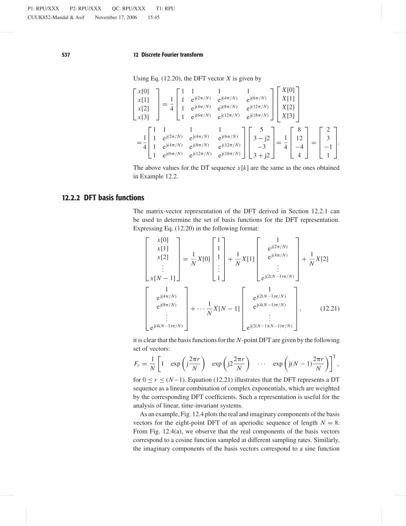
Using Eq. (12.20), the DFT vector X is given by

x[0]x[1]x[2]x[3]

= 1

4

1 1 1 11 e j(2/N ) e j(4/N ) e j(6/N )

1 e j(4/N ) e j(8/N ) e j(12/N )

1 e j(6/N ) e j(12/N ) e j(18/N )

X [0]X [1]X [2]X [3]

= 1

4

1 1 1 11 e j(2/N ) e j(4/N ) e j(6/N )

1 e j(4/N ) e j(8/N ) e j(12/N )

1 e j(6/N ) e j(12/N ) e j(18/N )

53 − j2−3

3 + j2

= 1

4

812−44

=

23

−11

.

The above values for the DT sequence x[k] are the same as the ones obtainedin Example 12.2.

12.2.2 DFT basis functions

The matrix-vector representation of the DFT derived in Section 12.2.1 canbe used to determine the set of basis functions for the DFT representation.Expressing Eq. (12.20) in the following format:

x[0]x[1]x[2]

...x[N − 1]

= 1

NX [0]

111...1

+ 1

NX [1]

1e j(2/N )

e j(4/N )

...e j(2(N−1)/N )

+ 1

NX [2]

1ej(4/N )

e j(8/N )

...e j(4(N−1)/N )

+ · · · 1

NX [N − 1]

1e j(2(N−1)/N )

e j(4(N−1)/N )

...e j(2(N−1)(N−1)/N )

, (12.21)

it is clear that the basis functions for the N -point DFT are given by the followingset of vectors:

Fr = 1

N

[1 exp

(j2r

N

)exp

(j2

2r

N

)· · · exp

(j(N − 1)

2r

N

)]T

,

for 0 ≤ r ≤ (N−1). Equation (12.21) illustrates that the DFT represents a DTsequence as a linear combination of complex exponentials, which are weightedby the corresponding DFT coefficients. Such a representation is useful for theanalysis of linear, time-invariant systems.

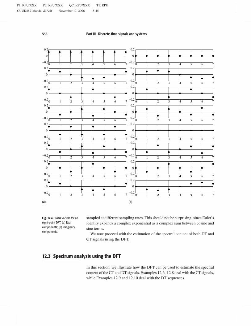
As an example, Fig. 12.4 plots the real and imaginary components of the basisvectors for the eight-point DFT of an aperiodic sequence of length N = 8.From Fig. 12.4(a), we observe that the real components of the basis vectorscorrespond to a cosine function sampled at different sampling rates. Similarly,the imaginary components of the basis vectors correspond to a sine function




−0.2

−0.2

−0.2

−0.2

−0.2

−0.2

−0.2

−0.2

−0.2

−0.2

−0.2

−0.2

−0.2

−0.2

−0.2

−0.2

0

0.2

0 1 2 3 4 5 6 7

0 1 2 3 4 5 6 7

0

0.2

0 1 2 3 4 5 6 7

0

0.2

0

0.2

0 1 2 3 4 5 6 7

0 1 2 3 4 5 6 7

0

0.2

0 1 2 3 4 5 6 7

0

0.2

0 1 2 3 4 5 6 7

0

0.2

0 1 2 3 4 5 6 7

0

0.2

0 1 2 3 4 5 6 7

0

0.2

0 1 2 3 4 5 6 7

0

0.2

0 1 2 3 4 5 6 7

0

0.2

0 1 2 3 4 5 6 7

0

0.2

0 1 2 3 4 5 6 7

0

0.2

0 1 2 3 4 5 6 7

0

0.2

0 1 2 3 4 5 6 7

0

0.2

0 1 2 3 4 5 6 7

0

0.2

11

4 54 5

1 2 3 51 2 3 5

(a)(a) (b)

Fig. 12.4. Basis vectors for aneight-point DFT. (a) Realcomponents; (b) imaginarycomponents.

sampled at different sampling rates. This should not be surprising, since Euler’sidentity expands a complex exponential as a complex sum between cosine andsine terms.

We now proceed with the estimation of the spectral content of both DT andCT signals using the DFT.

12.3 Spectrum analysis using the DFT

In this section, we illustrate how the DFT can be used to estimate the spectralcontent of the CT and DT signals. Examples 12.6–12.8 deal with the CT signals,while Examples 12.9 and 12.10 deal with the DT sequences.




Example 12.6Using the DFT, estimate the frequency characteristics of the decaying expo-nential signal g(t) = exp(−0.5t)u(t). Plot the magnitude and phase spectra.

SolutionFollowing the procedure outlined in Section 12.1, the three steps involved incomputing the CTFT are listed below.

Step 1: Impulse-train sampling Based on Table 5.1, the CTFT of the decay-ing exponential is given by

g(t) = e−0.5t u(t)CTFT←−−→ G() = 1

0.5 + j.

This CTFT pair implies that the bandwidth of g(t) is infinite. Ideally speaking,the Nyquist sampling theorem can never be satisfied for the decaying exponen-tial signal. However, we exploit the fact that the magnitude |G()| of the CTFTdecreases monotonically with higher frequencies and we neglect any frequencycomponents at which the magnitude falls below a certain threshold . Selectingthe value of = 0.01 × |G()|max, the threshold frequency B is given by∣∣∣ 1

0.5 + j2B

∣∣∣ ≤ 0.01 × |G()|max.

Since the maximum value of the magnitude |G()| is 2 at = 0, the aboveexpression reduces to √

0.25 + (2B)2 ≥ 50,

or B ≥ 7.95 Hz. The Nyquist sampling rate f1 is therefore given by

f1 ≥ 2 × 7.95 = 15.90 samples/s.

Selecting a sampling rate of f1 = 20 samples/s, or a sampling interval T1 =1/20 = 0.05 s, the DT approximation of the decaying exponential is given by

g[k] = g(kT1) = e−0.5kT1 u[k] = e−0.025ku[k].

Since there is a discontinuity at k = 0, we set g[0] = 0.5.

Step 2: Time-limitation To truncate the length of g[k], we apply a rectangularwindow of length N = 203 samples. The truncated sequence is given by

gw [k] = e−0.025k(u[k] − u[k − 199]) =

e−0.025k 0 ≤ k ≤ 2020 elsewhere.

The subscript w in gw [k] denotes the truncated version of g[k] obtained bymultiplying by the window function w[k]. Note that the truncated sequencegw [k] is a fairly good approximation of g[k], as the peak magnitude of thetruncated samples is given by 0.0063 and occurs at k = 203. This is only 0.63%of the peak value of the complex exponential g[k].




Step 3: DFT computation The DFT of the truncated DT sequence gw [k]can now be computed directly from Eq. (12.16). M A T L A B provides a built-infunction fft, which has the calling syntax of

>> G = fft(g);

where g is the signal vector containing the values of the DT sequence gw [k]and G is the computed DFT. Both g and G have a length of N , implying thatan N -point DFT is being taken. The built-in function fft computes the DFTwithin the frequency range 0 ≤ r ≤ (N−1). Since the DFT is periodic, we canobtain the DFT within the frequency range −(N − 1)/2 ≤ r ≤ (N − 1)/2 bya circular shift of the DFT coefficients. In M A T L A B , this is accomplished bythe fftshift function.

Having computed the DFT, we use Eq. (12.12) to estimate the CTFT of theoriginal CT decaying exponential signal g(t). The M A T L A B code for comput-ing the CTFT is as follows:

>> f1 = 20; t1 = 1/f1; % set sampling rate and interval

>> N = 203; k = 0:N-1; % set length of DT sequence to

N = 203

>> g = exp(-0.025*k); % compute the DT sequence

g(1) = 0.5;

>> G = fft(g); % determine the 203-point DFT

>> G = fftshift(G); % shift the DFT coefficients

>> G = t1*G; % scale DFT such that DFT = CTFT

>> w = -pi*f1:2*pi*f1/N:pi*f1-2*pi*f1/N; %compute CTFT

frequencies

>> stem(w,abs(G)); % plot CTFT magnitude spectrum

>> stem(w,angle(G)); % plot CTFT phase spectrum

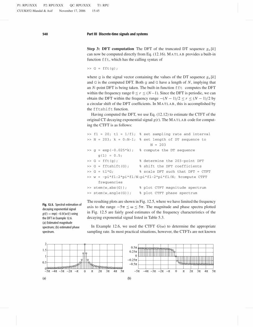
The resulting plots are shown in Fig. 12.5, where we have limited the frequencyaxis to the range −5 ≤ ≤ 5. The magnitude and phase spectra plottedin Fig. 12.5 are fairly good estimates of the frequency characteristics of thedecaying exponential signal listed in Table 5.3.

In Example 12.6, we used the CTFT G() to determine the appropriatesampling rate. In most practical situations, however, the CTFTs are not known

−5π −4π −3π −2π −π 0 π 2π 3π 4π 5π0

0.5

1

1.5

2

−5π −4π −3π −2π −π 0 π 2π 3π 4π 5π

−0.5π−0.25π

00.25π0.5π

(a) (b)

Fig. 12.5. Spectral estimation ofdecaying exponential signalg(t ) = exp(−0.5t )u(t ) usingthe DFT in Example 12.6.(a) Estimated magnitudespectrum; (b) estimated phasespectrum.




and one is forced to make an intelligent estimate of the bandwidth of the signal.If the frequency and time characteristics of the signal are not known, a highsampling rate and a large time window are arbitrarily chosen. In such cases, itis advised that a number of sampling rates and lengths be tried before finalizingthe estimates.

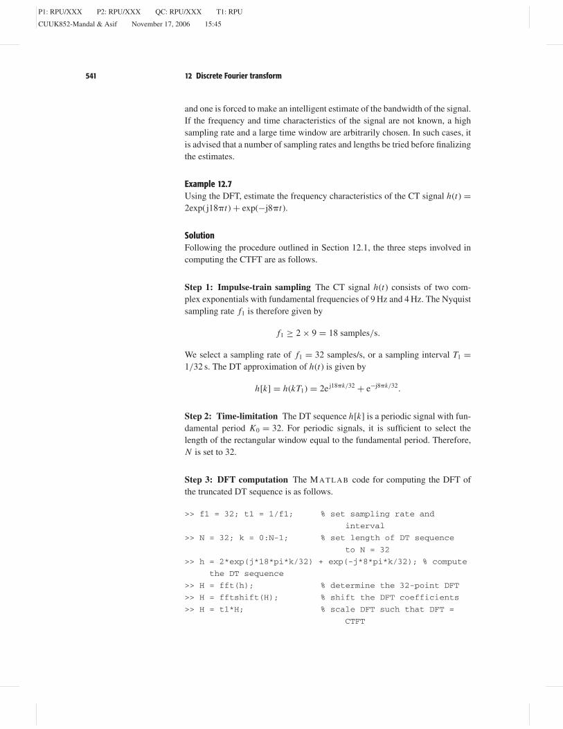
Example 12.7Using the DFT, estimate the frequency characteristics of the CT signal h(t) =2exp(j18t) + exp(−j8t).

SolutionFollowing the procedure outlined in Section 12.1, the three steps involved incomputing the CTFT are as follows.

Step 1: Impulse-train sampling The CT signal h(t) consists of two com-plex exponentials with fundamental frequencies of 9 Hz and 4 Hz. The Nyquistsampling rate f1 is therefore given by

f1 ≥ 2 × 9 = 18 samples/s.

We select a sampling rate of f1 = 32 samples/s, or a sampling interval T1 =1/32 s. The DT approximation of h(t) is given by

h[k] = h(kT1) = 2e j18k/32 + e−j8k/32.

Step 2: Time-limitation The DT sequence h[k] is a periodic signal with fun-damental period K0 = 32. For periodic signals, it is sufficient to select thelength of the rectangular window equal to the fundamental period. Therefore,N is set to 32.

Step 3: DFT computation The M A T L A B code for computing the DFT ofthe truncated DT sequence is as follows.

>> f1 = 32; t1 = 1/f1; % set sampling rate and

interval

>> N = 32; k = 0:N-1; % set length of DT sequence

to N = 32

>> h = 2*exp(j*18*pi*k/32) + exp(-j*8*pi*k/32); % compute

the DT sequence

>> H = fft(h); % determine the 32-point DFT

>> H = fftshift(H); % shift the DFT coefficients

>> H = t1*H; % scale DFT such that DFT =

CTFT




−30π −20π −10π 0 10π 20π 30π0

0.5

1

1.5

2

−30π −20π −10π 0 10π 20π 30π

−0.5π

0

0.5π

π

(a) (b)

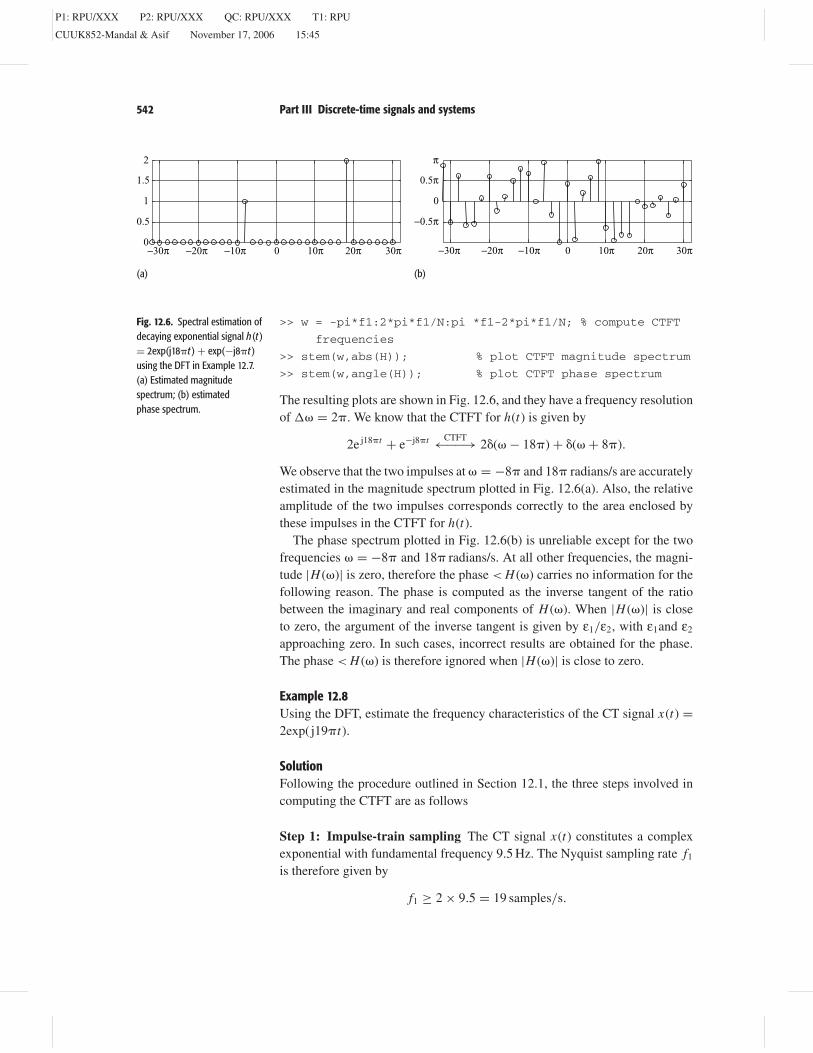
Fig. 12.6. Spectral estimation ofdecaying exponential signal h(t )= 2exp(j18t ) + exp(−j8t )using the DFT in Example 12.7.(a) Estimated magnitudespectrum; (b) estimatedphase spectrum.

>> w = -pi*f1:2*pi*f1/N:pi *f1-2*pi*f1/N; % compute CTFT

frequencies

>> stem(w,abs(H)); % plot CTFT magnitude spectrum

>> stem(w,angle(H)); % plot CTFT phase spectrum

The resulting plots are shown in Fig. 12.6, and they have a frequency resolutionof = 2. We know that the CTFT for h(t) is given by

2e j18t + e−j8t CTFT←−−→ 2( − 18) + ( + 8).

We observe that the two impulses at = −8 and 18 radians/s are accuratelyestimated in the magnitude spectrum plotted in Fig. 12.6(a). Also, the relativeamplitude of the two impulses corresponds correctly to the area enclosed bythese impulses in the CTFT for h(t).

The phase spectrum plotted in Fig. 12.6(b) is unreliable except for the twofrequencies = −8 and 18 radians/s. At all other frequencies, the magni-tude |H ()| is zero, therefore the phase < H () carries no information for thefollowing reason. The phase is computed as the inverse tangent of the ratiobetween the imaginary and real components of H (). When |H ()| is closeto zero, the argument of the inverse tangent is given by ε1/ε2, with ε1and ε2

approaching zero. In such cases, incorrect results are obtained for the phase.The phase < H () is therefore ignored when |H ()| is close to zero.

Example 12.8Using the DFT, estimate the frequency characteristics of the CT signal x(t) =2exp(j19t).

SolutionFollowing the procedure outlined in Section 12.1, the three steps involved incomputing the CTFT are as follows

Step 1: Impulse-train sampling The CT signal x(t) constitutes a complexexponential with fundamental frequency 9.5 Hz. The Nyquist sampling rate f1

is therefore given by

f1 ≥ 2 × 9.5 = 19 samples/s.




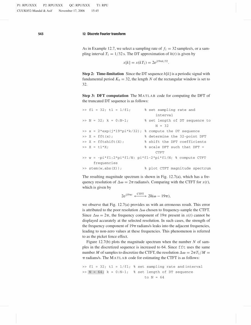
As in Example 12.7, we select a sampling rate of f1 = 32 samples/s, or a sam-pling interval T1 = 1/32 s. The DT approximation of h(t) is given by

x[k] = x(kT1) = 2e j19k/32.

Step 2: Time-limitation Since the DT sequence h[k] is a periodic signal withfundamental period K0 = 32, the length N of the rectangular window is set to32.

Step 3: DFT computation The M A T L A B code for computing the DFT ofthe truncated DT sequence is as follows:

>> f1 = 32; t1 = 1/f1; % set sampling rate and

interval

>> N = 32; k = 0:N-1; % set length of DT sequence to

N = 32

>> x = 2*exp(j*19*pi*k/32); % compute the DT sequence

>> X = fft(x); % determine the 32-point DFT

>> X = fftshift(X); % shift the DFT coefficients

>> X = t1*X; % scale DFT such that DFT =

CTFT

>> w = -pi*f1:2*pi*f1/N: pi*f1-2*pi*f1/N; % compute CTFT

frequencies

>> stem(w,abs(X)); % plot CTFT magnitude spectrum

The resulting magnitude spectrum is shown in Fig. 12.7(a), which has a fre-quency resolution of = 2 radians/s. Comparing with the CTFT for x(t),which is given by

2e j19t CTFT←−−→ 2( − 19),

we observe that Fig. 12.7(a) provides us with an erroneous result. This erroris attributed to the poor resolution chosen to frequency-sample the CTFT.Since = 2, the frequency component of 19 present in x(t) cannot bedisplayed accurately at the selected resolution. In such cases, the strength ofthe frequency component of 19 radians/s leaks into the adjacent frequencies,leading to non-zero values at these frequencies. This phenomenon is referredto as the picket fence effect.

Figure 12.7(b) plots the magnitude spectrum when the number N of sam-ples in the discretized sequence is increased to 64. Since fft uses the samenumber M of samples to discretize the CTFT, the resolution = 2T1/M = radians/s. The M A T L A B code for estimating the CTFT is as follows:

>> f1 = 32; t1 = 1/f1; % set sampling rate and interval


to N = 64




−30π −20π −10π 0 10π 20π 30π0

0.5

1

1.5

2

−30π −20π −10π 0 10π 20π 30π0

0.5

1

1.5

2

(a) (b)

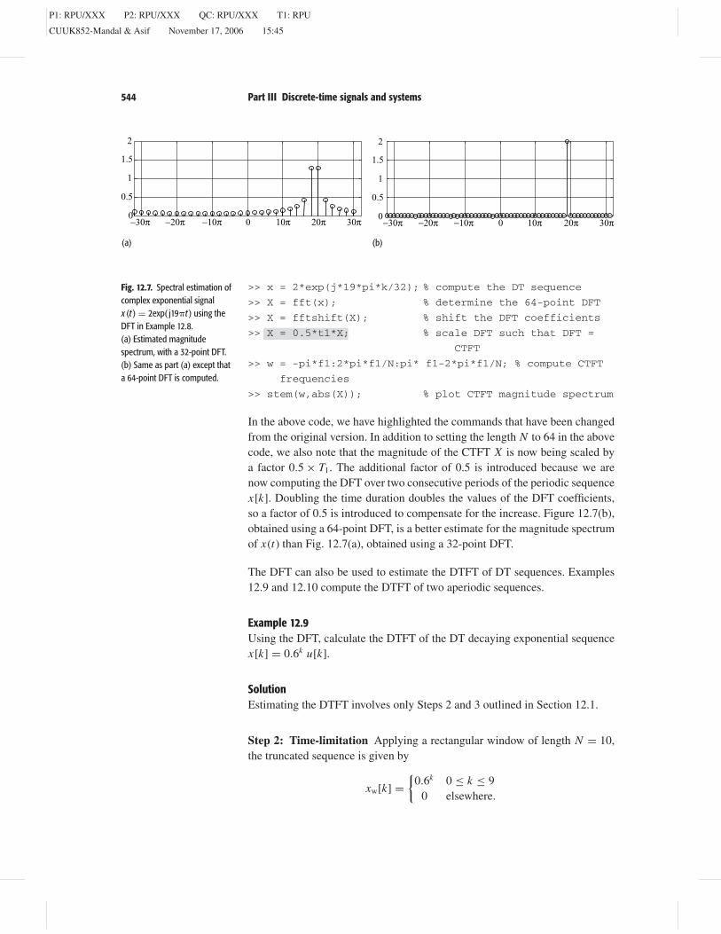
Fig. 12.7. Spectral estimation ofcomplex exponential signalx (t ) = 2exp( j19t ) using theDFT in Example 12.8.(a) Estimated magnitudespectrum, with a 32-point DFT.(b) Same as part (a) except thata 64-point DFT is computed.

>> x = 2*exp(j*19*pi*k/32); % compute the DT sequence



>> X = 0.5*t1*X; % scale DFT such that DFT =

CTFT

>> w = -pi*f1:2*pi*f1/N:pi* f1-2*pi*f1/N; % compute CTFT

frequencies

>> stem(w,abs(X)); % plot CTFT magnitude spectrum

In the above code, we have highlighted the commands that have been changedfrom the original version. In addition to setting the length N to 64 in the abovecode, we also note that the magnitude of the CTFT X is now being scaled bya factor 0.5 × T1. The additional factor of 0.5 is introduced because we arenow computing the DFT over two consecutive periods of the periodic sequencex[k]. Doubling the time duration doubles the values of the DFT coefficients,so a factor of 0.5 is introduced to compensate for the increase. Figure 12.7(b),obtained using a 64-point DFT, is a better estimate for the magnitude spectrumof x(t) than Fig. 12.7(a), obtained using a 32-point DFT.

The DFT can also be used to estimate the DTFT of DT sequences. Examples12.9 and 12.10 compute the DTFT of two aperiodic sequences.

Example 12.9Using the DFT, calculate the DTFT of the DT decaying exponential sequencex[k] = 0.6k u[k].

SolutionEstimating the DTFT involves only Steps 2 and 3 outlined in Section 12.1.

Step 2: Time-limitation Applying a rectangular window of length N = 10,the truncated sequence is given by

xw[k] =

0.6k 0 ≤ k ≤ 90 elsewhere.




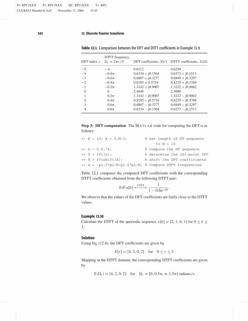
Table 12.1. Comparison between the DFT and DTFT coefficients in Example 12.9

DTFT frequency,DFT index, r r = 2r/N DFT coefficients, X [r ] DTFT coefficients, X ()

−5 − 0.6212 0.6250−4 −0.8 0.6334 + j0.1504 0.6373 + j0.1513−3 −0.6 0.6807 + j0.3277 0.6849 + j0.3297−2 −0.4 0.8185 + 0.5734 0.8235 + j0.5769−1 −0.2 1.3142 + j0.9007 1.3222 + j0.9062

0 0 2.4848 2.50001 0.2 1.3142 − j0.9007 1.3222 − j0.90622 0.4 0.8185 − j0.5734 0.8235 − j0.57693 0.6 0.6807 − j0.3277 0.6849 − j0.32974 0.8 0.6334 − j0.1504 0.6373 − j0.1513

Step 3: DFT computation The M A T L A B code for computing the DFT is asfollows:


to N = 10

>> x = 0.6.ˆk; % compute the DT sequence



>> w = -pi:2*pi/N:pi-2*pi/N; % compute DTFT frequencies

Table 12.1 compares the computed DFT coefficients with the correspondingDTFT coefficients obtained from the following DTFT pair:

0.6ku[k]CTFT←−−→ 1

1 − 0.6e−j.

We observe that the values of the DFT coefficients are fairly close to the DTFTvalues.

Example 12.10Calculate the DTFT of the aperiodic sequence x[k] = [2, 1, 0, 1] for 0 ≤ k ≤3.

SolutionUsing Eq. (12.6), the DFT coefficients are given by

X [r ] = [4, 2, 0, 2] for 0 ≤ r ≤ 3.

Mapping in the DTFT domain, the corresponding DTFT coefficients are givenby

X (r ) = [4, 2, 0, 2] for r = [0, 0.5, , 1.5] radians/s.




−π −0.75π −0.5π −0.25π 0 0.25π 0.5π 0.75π0

1

2

3

4

−π −0.75π −0.5π −0.25π 0 0.25π 0.5π 0.75π π−0.5π

−0.25π

0

0.25π

0.5π

π

(a) (b)

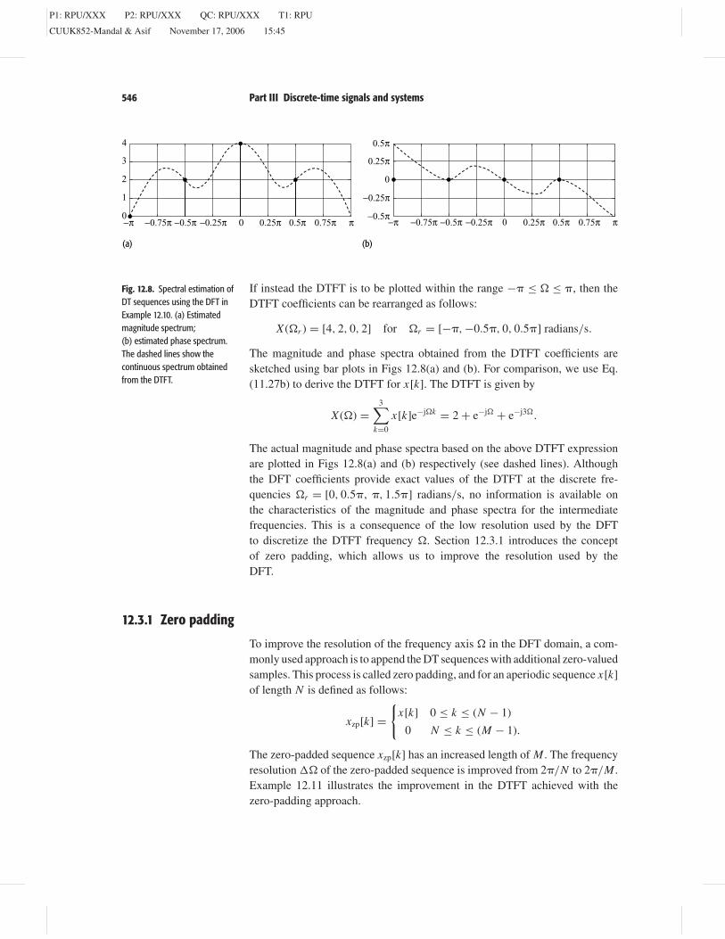
Fig. 12.8. Spectral estimation ofDT sequences using the DFT inExample 12.10. (a) Estimatedmagnitude spectrum;(b) estimated phase spectrum.The dashed lines show thecontinuous spectrum obtainedfrom the DTFT.

If instead the DTFT is to be plotted within the range − ≤ ≤ , then theDTFT coefficients can be rearranged as follows:

X (r ) = [4, 2, 0, 2] for r = [−, −0.5, 0, 0.5] radians/s.

The magnitude and phase spectra obtained from the DTFT coefficients aresketched using bar plots in Figs 12.8(a) and (b). For comparison, we use Eq.(11.27b) to derive the DTFT for x[k]. The DTFT is given by

X () =3∑

k=0

x[k]e−jk = 2 + e−j + e−j3.

The actual magnitude and phase spectra based on the above DTFT expressionare plotted in Figs 12.8(a) and (b) respectively (see dashed lines). Althoughthe DFT coefficients provide exact values of the DTFT at the discrete fre-quencies r = [0, 0.5, , 1.5] radians/s, no information is available onthe characteristics of the magnitude and phase spectra for the intermediatefrequencies. This is a consequence of the low resolution used by the DFTto discretize the DTFT frequency . Section 12.3.1 introduces the conceptof zero padding, which allows us to improve the resolution used by theDFT.

12.3.1 Zero padding

To improve the resolution of the frequency axis in the DFT domain, a com-monly used approach is to append the DT sequences with additional zero-valuedsamples. This process is called zero padding, and for an aperiodic sequence x[k]of length N is defined as follows:

xzp[k] =

x[k] 0 ≤ k ≤ (N − 1)

0 N ≤ k ≤ (M − 1).

The zero-padded sequence xzp[k] has an increased length of M . The frequencyresolution of the zero-padded sequence is improved from 2/N to 2/M .Example 12.11 illustrates the improvement in the DTFT achieved with thezero-padding approach.




−π −0.75π −0.5π −0.25π 0 0.25π 0.5π 0.75π0

1

2

3

4

−π −0.75π −0.5π −0.25π 0 0.25π 0.5π 0.75π−0.5π

−0.25π0

0.25π0.5π

π π

(a) (b)

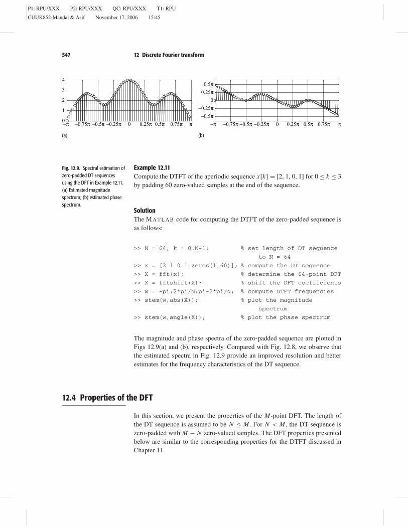
Fig. 12.9. Spectral estimation ofzero-padded DT sequencesusing the DFT in Example 12.11.(a) Estimated magnitudespectrum; (b) estimated phasespectrum.

Example 12.11Compute the DTFT of the aperiodic sequence x[k] = [2, 1, 0, 1] for 0 ≤ k ≤ 3by padding 60 zero-valued samples at the end of the sequence.

SolutionThe M A T L A B code for computing the DTFT of the zero-padded sequence isas follows:


to N = 64

>> x = [2 1 0 1 zeros(1,60)]; % compute the DT sequence



>> w = -pi:2*pi/N:pi-2*pi/N; % compute DTFT frequencies

>> stem(w,abs(X)); % plot the magnitude

spectrum

>> stem(w,angle(X)); % plot the phase spectrum

The magnitude and phase spectra of the zero-padded sequence are plotted inFigs 12.9(a) and (b), respectively. Compared with Fig. 12.8, we observe thatthe estimated spectra in Fig. 12.9 provide an improved resolution and betterestimates for the frequency characteristics of the DT sequence.

12.4 Properties of the DFT

In this section, we present the properties of the M-point DFT. The length ofthe DT sequence is assumed to be N ≤ M . For N < M , the DT sequence iszero-padded with M − N zero-valued samples. The DFT properties presentedbelow are similar to the corresponding properties for the DTFT discussed inChapter 11.




12.4.1 Periodicity

The M-point DFT of an aperiodic DT sequence with length N with M ≥ N isitself periodic with period M . In other words,

X [r ] = X [r + pM], (12.22)

for 0 ≤ r ≤ (M − 1) with p ∈ R+.

12.4.2 Orthogonality

The column vectors Fr of the DFT matrix F , defined in Eq. (12.21), form thebasis vectors of the DFT and are orthogonal with respect to each other such that

FHr · Fq =

M for r = q0 for r = q,

where (·) represents the dot product and the superscript H represents the Her-mitian operation.

12.4.3 Linearity

If x1[k] and x2[k] are two DT sequences with the following M-point DFT pairs:

x1[k]DFT←−−→ X1[r ] and x2[k]

DFT←−−→ X2[r ],

then the linearity property states that

a1x1[k] + a2x2[k]DFT←−−→ a1 X1[r ] + a2 X2[r ], (12.23)

for any arbitrary constants a1 and a2, which may be complex-valued.

12.4.4 Hermitian symmetry

The M-point DFT X [r ] of a real-valued aperiodic sequence x[k] is conjugate-symmetric about r = M/2. Mathematically, the Hermitian symmetry impliesthat

X [r ] = X∗[M − r ], (12.24)

where X∗[r ] denotes the complex conjugate of X [r ].In terms of the magnitude and phase spectra of the DFT X [r ], the Hermitian

symmetry property can be expressed as follows:

|X [M − r ]| = |X [r ]| and < X [M − r ] = − < X [r ], (12.25)

implying that the magnitude spectrum is even and that the phase spectrum isodd.

The validity of the Hermitian symmetry can be observed in the DFT plottedfor various aperiodic sequences in Examples 12.2–12.11.




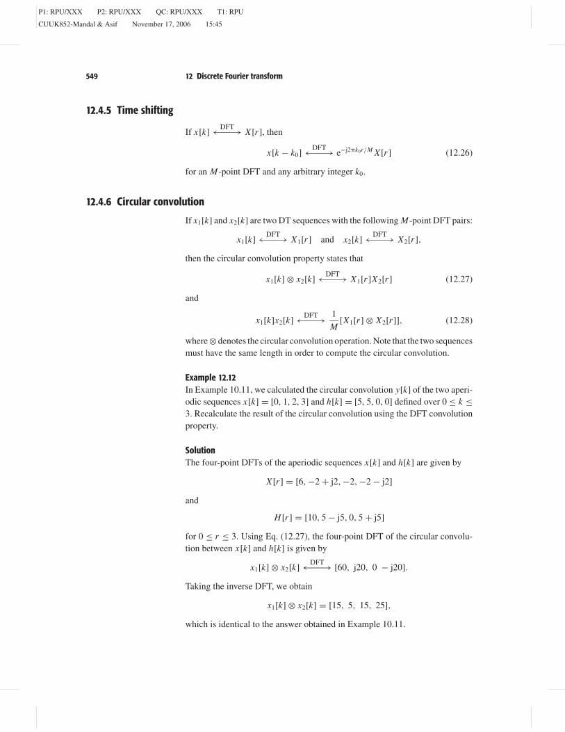
12.4.5 Time shifting

If x[k]DFT←−−→ X [r ], then

x[k − k0]DFT←−−→ e−j2k0r/M X [r ] (12.26)

for an M-point DFT and any arbitrary integer k0.

12.4.6 Circular convolution

If x1[k] and x2[k] are two DT sequences with the following M-point DFT pairs:

x1[k]DFT←−−→ X1[r ] and x2[k]

DFT←−−→ X2[r ],

then the circular convolution property states that

x1[k] ⊗ x2[k]DFT←−−→ X1[r ]X2[r ] (12.27)

and

x1[k]x2[k]DFT←−−→ 1

M[X1[r ] ⊗ X2[r ]], (12.28)

where ⊗ denotes the circular convolution operation. Note that the two sequencesmust have the same length in order to compute the circular convolution.

Example 12.12In Example 10.11, we calculated the circular convolution y[k] of the two aperi-odic sequences x[k] = [0, 1, 2, 3] and h[k] = [5, 5, 0, 0] defined over 0 ≤ k ≤3. Recalculate the result of the circular convolution using the DFT convolutionproperty.

SolutionThe four-point DFTs of the aperiodic sequences x[k] and h[k] are given by

X [r ] = [6, −2 + j2, −2, −2 − j2]

and

H [r ] = [10, 5 − j5, 0, 5 + j5]

for 0 ≤ r ≤ 3. Using Eq. (12.27), the four-point DFT of the circular convolu-tion between x[k] and h[k] is given by

x1[k] ⊗ x2[k]DFT←−−→ [60, j20, 0 − j20].

Taking the inverse DFT, we obtain

x1[k] ⊗ x2[k] = [15, 5, 15, 25],

which is identical to the answer obtained in Example 10.11.




12.4.7 Parseval’s theorem

If x[k]DFT←−−→ X [r ], then the energy of the aperiodic sequence x[k] of length

N can be expressed in terms of its M-point DFT as follows:

Ex =N−1∑k=0

|x[k]|2 = 1

M

M−1∑k=0

|X [r ]|2. (12.29)

Parseval’s theorem shows that the DFT preserves the energy of the signal withina scale factor of M .

12.5 Convolution using the DFT

In Section 10.6.1, we showed that the linear convolution x1[k] ∗ x2[k] betweentwo time-limited DT sequences x1[k] and x2[k] of lengths K1 and K2, respec-tively, can be expressed in terms of the circular convolution x1[k] ⊗x2[k]. Theprocedure requires zero padding both x1[k] and x2[k] to have individual lengthsof K ≥ (K1 + K2 – 1). It was shown that the result of the circular convolutionof the zero-padded sequences is the same as that of the linear convolution.

Since computationally efficient algorithms are available for computing theDFT of a finite-duration sequence, the circular convolution property can beexploited to implement the linear convolution of the two sequences x1[k] andx2[k] using the following procedure.

(1) Compute the K -point DFTs X1[r ] and X2[r ] of the two time-limitedsequences x1[k] and x2[k]. The value of K is lower bounded by (K1 + K2

– 1), i.e. K ≥ (K1 + K2 – 1).(2) Compute the product X3[r ] = X1[r ]X2[r ] for 0 ≤ r ≤ K − 1.(3) Compute the sequence x3[k] as the inverse DFT of X3[r ]. The resulting

sequence x3[k] is the result of the linear convolution between x1[k] andx2[k].

The above approach is explained in Example 12.13.

Example 12.13Example 10.13 computed the linear convolution of the following DT sequences:

x[k] =

2 k = 0−1 |k| = 1

0 otherwiseand h[k] =

2 k = 03 |k| = 1

−1 |k| = 20 otherwise,

using the circular convolution method outlined in Algorithm 10.4 inSection 10.6.1. Repeat Example 10.13 using the DFT-based approach describedabove.




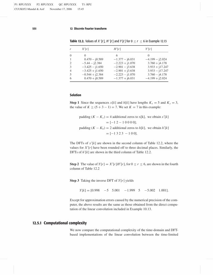
Table 12.2. Values of X ′[r ], H ′[r ] and Y [r ] for 0 ≤ r ≤ 6 in Example 12.13

r X ′[r ] H ′[r ] Y ′[r ]

0 0 6 01 0.470 − j0.589 −1.377 − j6.031 −4.199 − j2.0242 −5.44 − j2.384 −2.223 + j1.070 3.760 + j4.1783 −3.425 − j1.650 −2.901 − j3.638 3.933 + j17.2474 −3.425 + j1.650 −2.901 + j3.638 3.933 − j17.2475 −0.544 + j2.384 −2.223 − j1.070 3.760 − j4.1786 0.470 + j0.589 −1.377 + j6.031 −4.199 + j2.024

Solution

Step 1 Since the sequences x[k] and h[k] have lengths Kx = 5 and Ky = 3,the value of K ≥ (5 + 3 − 1) = 7. We set K = 7 in this example:

padding (K − Kx ) = 4 additional zeros to x[k], we obtain x ′[k]

= [−1 2 − 1 0 0 0 0];

padding (K − Kh) = 2 additional zeros to h[k], we obtain h′[k]

= [−1 3 2 3 − 1 0 0].

The DFTs of x ′[k] are shown in the second column of Table 12.2, where thevalues for X ′[r ] have been rounded off to three decimal places. Similarly, theDFTs of h′[k] are shown in the third column of Table 12.2.

Step 2 The value of Y [r ] = X ′[r ]H ′[r ], for 0 ≤ r ≤ 6, are shown in the fourthcolumn of Table 12.2

Step 3 Taking the inverse DFT of Y [r ] yields

Y [k] = [0.998 −5 5.001 −1.999 5 −5.002 1.001].

Except for approximation errors caused by the numerical precision of the com-puter, the above results are the same as those obtained from the direct compu-tation of the linear convolution included in Example 10.13.

12.5.1 Computational complexity

We now compare the computational complexity of the time-domain and DFT-based implementations of the linear convolution between the time-limited




sequences x1[k] and x2[k] with lengths K1 and K2, respectively. For simplicity,we assume that x1[k] and x2[k] are real-valued sequences with lengths K1 andK2, respectively.

Time-domain approach This is based on the direct computation of the con-volution sum

y[k] = x1[k] ∗ x1[k] =∞∑

m=−∞x1[m]x2[k − m],

which requires roughly K1 × K2 multiplications and K1 × K2 additions. Thetotal number of floating point operations (flops) required with the time-domainapproach is therefore given by 2K1 × K2.

DFT-based approach Step 1 of the DFT-based approach computes two K =K1 + K2 − 1 point DFTs of the DT sequences x1[k] and x2[k]. In Section 12.6,we show that a K -point DFT can be implemented using fast Fourier trans-form (FFT) techniques with 0.5K log2 K complex multiplications and K log2 Kcomplex additions. Since each complex multiplication requires four scalar mul-tiplications and two scalar additions, a total of six flops are required per com-plex multiplication. Each complex addition, on the other hand, requires twoscalar additions, leading to two flops per complex addition. Therefore, Step 1of the DFT-based approach requires a total of 2×[3K log2 K + 2K log2 K ] =10K log2 K flops.

Step 2 multiplies DFTs for x1[k] and x2[k]. Each DFT has a length ofK = K1 + K2 − 1 points; therefore, a total of K complex multiplications andK − 1 ≈ K complex additions are required. The total number of computationsrequired in Step 1 is therefore given by 8K or 8(K1 + K2 – 1) flops.

Step 3 computes one inverse DFT based on the FFT implementation requiring5K log2K flops.

The total number of flops required with the DFT-based approach is thereforegiven by

15K log2 K + 6K ≈ 15K log2 K flops,

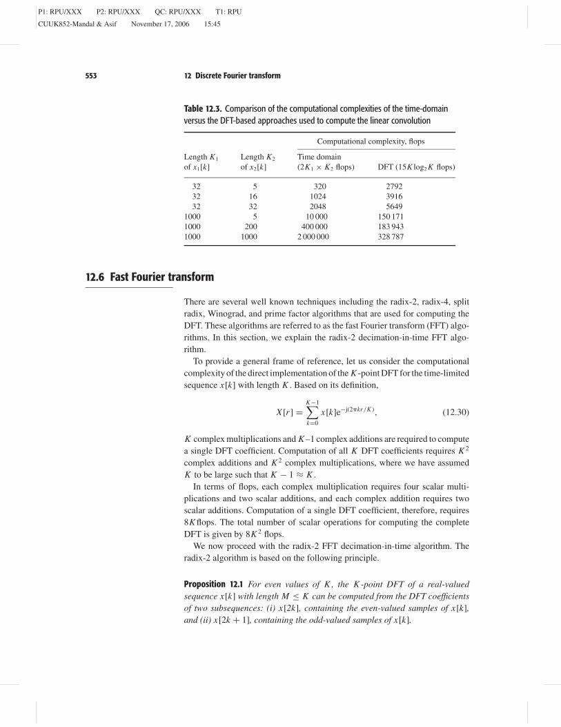
where K = K1 + K2 − 1. Assuming K1 = K2, the DFT-based approach pro-vides a computation saving of O(log2 K/K ) in comparison with the direct com-putation of the convolution sum in the time domain. Table 12.3 compares thecomputational complexity of the two approaches for a few selected values ofK1 and K2. We observe that for sequences with lengths greater than 1000samples, the DFT-based approach provides significant savings over the directcomputation of the circular convolution in the time domain.




Table 12.3. Comparison of the computational complexities of the time-domainversus the DFT-based approaches used to compute the linear convolution

Computational complexity, flops

Length K1

of x1[k]Length K2

of x2[k]Time domain(2K1 × K2 flops) DFT (15K log2 K flops)

32 5 320 279232 16 1024 391632 32 2048 5649

1000 5 10 000 150 1711000 200 400 000 183 9431000 1000 2 000 000 328 787

12.6 Fast Fourier transform

There are several well known techniques including the radix-2, radix-4, splitradix, Winograd, and prime factor algorithms that are used for computing theDFT. These algorithms are referred to as the fast Fourier transform (FFT) algo-rithms. In this section, we explain the radix-2 decimation-in-time FFT algo-rithm.

To provide a general frame of reference, let us consider the computationalcomplexity of the direct implementation of the K -point DFT for the time-limitedsequence x[k] with length K . Based on its definition,

X [r ] =K−1∑k=0

x[k]e−j(2kr/K ), (12.30)

K complex multiplications and K –1 complex additions are required to computea single DFT coefficient. Computation of all K DFT coefficients requires K 2

complex additions and K 2 complex multiplications, where we have assumedK to be large such that K − 1 ≈ K .

In terms of flops, each complex multiplication requires four scalar multi-plications and two scalar additions, and each complex addition requires twoscalar additions. Computation of a single DFT coefficient, therefore, requires8K flops. The total number of scalar operations for computing the completeDFT is given by 8K 2 flops.

We now proceed with the radix-2 FFT decimation-in-time algorithm. Theradix-2 algorithm is based on the following principle.

Proposition 12.1 For even values of K , the K -point DFT of a real-valuedsequence x[k] with length M ≤ K can be computed from the DFT coefficientsof two subsequences: (i) x[2k], containing the even-valued samples of x[k],and (ii) x[2k + 1], containing the odd-valued samples of x[k].




ProofExpressing Eq. (12.30) in terms of real- and odd-numbered-valued samples ofx[k], we obtain

X [r ] =K−1∑

k=0,2,4,...

x[k]e−j(2kr/K )

︸︷︷︸Term I

+K−1∑

k=1,3,5,...

x[k]e−j(2kr/K )

︸︷︷︸Term II

, (12.31)

for 0 ≤ r ≤ (M − 1). Substituting k = 2m in Term I and k = 2m + 1 in Term II,Eq. (12.31) can be expressed as follows:

X [r ] =K/2−1∑

m=0,1,2,...

x[2m]e−j(2(2m)r/K ) +K/2−1∑

m=0,1,2,...

x[2m + 1]e−j(2(2m+1)r/K )

or

X [r ] =K/2−1∑

m=0,1,2,...

x[2m]e−j(2mr/(K/2)) + e−j(2r/K )

K/2−1∑m=0,1,2,...

x[2m + 1]e−j(2mr/(K/2)), (12.32)

where exp[−j2(2m)r/K ] = exp[−j2mr/(K/2)]. By expressing g[m] =x[2m] and h[m] = x[2m + 1], we can express Eq. (12.32) in terms of the DFTsof g[m] and h[m]:

X [r ] =K/2−1∑

m=0,1,2,...

g[m]e−j(2mr/(K/2))

︸︷︷︸G[r ]

+ e−j(2r/K )K/2−1∑

m=0,1,2,...

h[m]e−j(2mr/(K/2))

︸︷︷︸H [r ]

(12.33)

or

X [r ] = G[r ] + W rK H [r ], (12.34a)

where WK is defined as exp(−j2/N ) and is referred to as the twiddle factor.The (K/2)-point DFTs G[r ] and H [r ] are defined as follows:

G[r ]=K/2−1∑

m=0,1,2,...

g[m]e−j(2mr/(K/2)) and H [r ] =K/2−1∑

m=0,1,2,...

h[m]e−j(2mr/(K/2)).

(12.34b)

Equation (12.34b) implies that G[r ] represents the (K/2)-point DFT coeffi-cients of g[k], the even-numbered samples of x[k]. Similarly, H [r ] representsthe (K/2)-point DFT coefficients of h[k], the odd-numbered samples of x[k].Equations (12.34) prove Proposition 12.6.1.

Based on Eqs (12.34), the procedure for determining the K -point DFT can besummarized by the following steps.




W1K

W2K

W3K

W4K

W6K

W5K

W7K

W0K

x[0]

x[2]

x[4]

x[6]

x[1]

x[3]

x[5]

x[7]

G[0]

G[1]

G[3]

G[4]

H[1]

H[2]

H[3]

H[4]

X [0]

X [1]

X [2]

X [3]

X [4]

X[5]

X [6]

X [7]

K/2 pointDFT

K/2 pointDFT

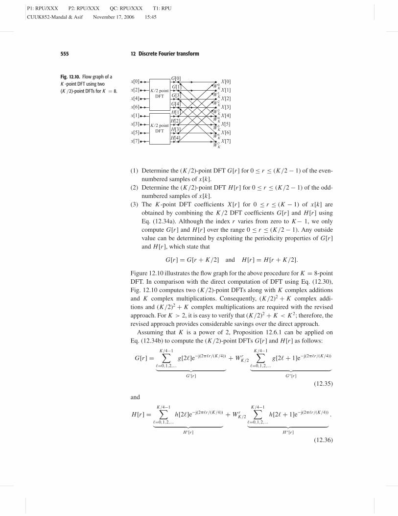
Fig. 12.10. Flow graph of aK -point DFT using two(K /2)-point DFTs for K = 8.

(1) Determine the (K/2)-point DFT G[r ] for 0 ≤ r ≤ (K/2 − 1) of the even-numbered samples of x[k].

(2) Determine the (K/2)-point DFT H [r ] for 0 ≤ r ≤ (K/2 − 1) of the odd-numbered samples of x[k].

(3) The K -point DFT coefficients X [r ] for 0 ≤ r ≤ (K − 1) of x[k] areobtained by combining the K/2 DFT coefficients G[r ] and H [r ] usingEq. (12.34a). Although the index r varies from zero to K− 1, we onlycompute G[r ] and H [r ] over the range 0 ≤ r ≤ (K/2 − 1). Any outsidevalue can be determined by exploiting the periodicity properties of G[r ]and H [r ], which state that

G[r ] = G[r + K/2] and H [r ] = H [r + K/2].

Figure 12.10 illustrates the flow graph for the above procedure for K = 8-pointDFT. In comparison with the direct computation of DFT using Eq. (12.30),Fig. 12.10 computes two (K/2)-point DFTs along with K complex additionsand K complex multiplications. Consequently, (K/2)2 + K complex addi-tions and (K/2)2 + K complex multiplications are required with the revisedapproach. For K > 2, it is easy to verify that (K/2)2 + K < K 2; therefore, therevised approach provides considerable savings over the direct approach.

Assuming that K is a power of 2, Proposition 12.6.1 can be applied onEq. (12.34b) to compute the (K/2)-point DFTs G[r ] and H [r ] as follows:

G[r ] =K/4−1∑

=0,1,2,...

g[2]e−j(2r/(K/4))

︸︷︷︸G ′[r ]

+ W rK/2

K/4−1∑=0,1,2,...

g[2 + 1]e−j(2r/(K/4))

︸︷︷︸G ′′[r ]

(12.35)

and

H [r ] =K/4−1∑

=0,1,2,...

h[2]e−j(2r/(K/4))

︸︷︷︸H ′[r ]

+ W rK/2

K/4−1∑=0,1,2,...

h[2 + 1]e−j(2r/(K/4))

︸︷︷︸H ′′[r ]

.

(12.36)




x[0]

x[4]

x[2]

x[6]

G[0]

G[1]

G[2]

G[3]

02/KW

12/KW

22/KW

32/KW

K/4 pointDFT

K/4 pointDFT

K/4 pointDFT

K/4 pointDFT

G′[0]

G′′[0]

G′′[1]

G′[1]

[1]x

[5]x

[3]x

x[7]

H [0]

H [1]

H [2]

H [3]

0K/2W

1K/2W2

K/2W

3K/2W

H ′ [0]

H ′ [1]

H ′′ [0]

H ′′ [1]

(a) (b)

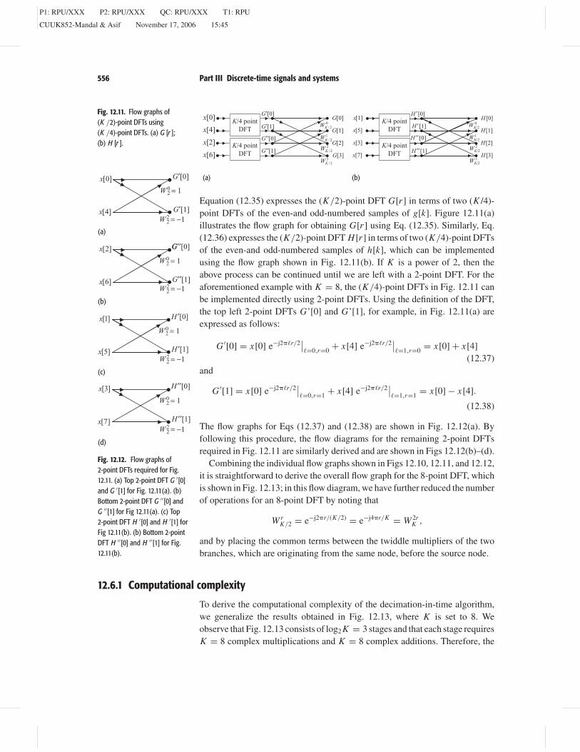
Fig. 12.11. Flow graphs of(K /2)-point DFTs using(K /4)-point DFTs. (a) G [r ];(b) H [r ].

Equation (12.35) expresses the (K/2)-point DFT G[r ] in terms of two (K /4)-point DFTs of the even-and odd-numbered samples of g[k]. Figure 12.11(a)illustrates the flow graph for obtaining G[r ] using Eq. (12.35). Similarly, Eq.(12.36) expresses the (K/2)-point DFT H [r ] in terms of two (K/4)-point DFTsof the even-and odd-numbered samples of h[k], which can be implementedusing the flow graph shown in Fig. 12.11(b). If K is a power of 2, then theabove process can be continued until we are left with a 2-point DFT. For theaforementioned example with K = 8, the (K/4)-point DFTs in Fig. 12.11 canbe implemented directly using 2-point DFTs. Using the definition of the DFT,the top left 2-point DFTs G’[0] and G’[1], for example, in Fig. 12.11(a) areexpressed as follows:

G ′[0] = x[0] e−j2r/2∣∣=0,r=0 + x[4] e−j2r/2

∣∣=1,r=0 = x[0] + x[4]

(12.37)and

G ′[1] = x[0] e−j2r/2∣∣=0,r=1 + x[4] e−j2r/2

∣∣=1,r=1 = x[0] − x[4].

(12.38)

The flow graphs for Eqs (12.37) and (12.38) are shown in Fig. 12.12(a). Byfollowing this procedure, the flow diagrams for the remaining 2-point DFTsrequired in Fig. 12.11 are similarly derived and are shown in Figs 12.12(b)–(d).

Combining the individual flow graphs shown in Figs 12.10, 12.11, and 12.12,it is straightforward to derive the overall flow graph for the 8-point DFT, whichis shown in Fig. 12.13; in this flow diagram, we have further reduced the numberof operations for an 8-point DFT by noting that

W rK/2 = e−j2r/(K/2) = e−j4r/K = W 2r

K ,

and by placing the common terms between the twiddle multipliers of the two

]1[x

]5[x

G]2[x

]6[x

G′[0]

G′[1]

G′′[0]

G′′[1]

H ′[0]

H ′[1]

H ′′[0]

H ′′[1]

W22 = −1

W22 = −1

W22 = −1

W22 = −1

W02 = 1

W02 = 1

W02 = 1

W02 = 1

]0[x

]4[x

]3[x

]7[x

(a)

(b)

(c)

(d)

Fig. 12.12. Flow graphs of2-point DFTs required for Fig.12.11. (a) Top 2-point DFT G ′[0]and G ′[1] for Fig. 12.11(a). (b)Bottom 2-point DFT G ′′[0] andG ′′[1] for Fig 12.11(a). (c) Top2-point DFT H ′[0] and H ′[1] forFig 12.11(b). (b) Bottom 2-pointDFT H ′′[0] and H ′′[1] for Fig.12.11(b). branches, which are originating from the same node, before the source node.

12.6.1 Computational complexity

To derive the computational complexity of the decimation-in-time algorithm,we generalize the results obtained in Fig. 12.13, where K is set to 8. Weobserve that Fig. 12.13 consists of log2 K = 3 stages and that each stage requiresK = 8 complex multiplications and K = 8 complex additions. Therefore, the




stage 1 stage 3

x[0]

x[4]

x[2]

x[6]

x[1]

x[5]

x[3]

x[7]

]0[X

]1[X

]2[X

]3[X

]4[X

]5[X

]6[X

]7[X

4KW

4KW

4KW

4KW

0KW

2KW

0KW

2KW

4KW

4KW

4KW

4KW

0KW

1KW

2KW

3KW

4KW

4KW

4KW

4KW

0KW

0KW

0KW

0KW

stage 2

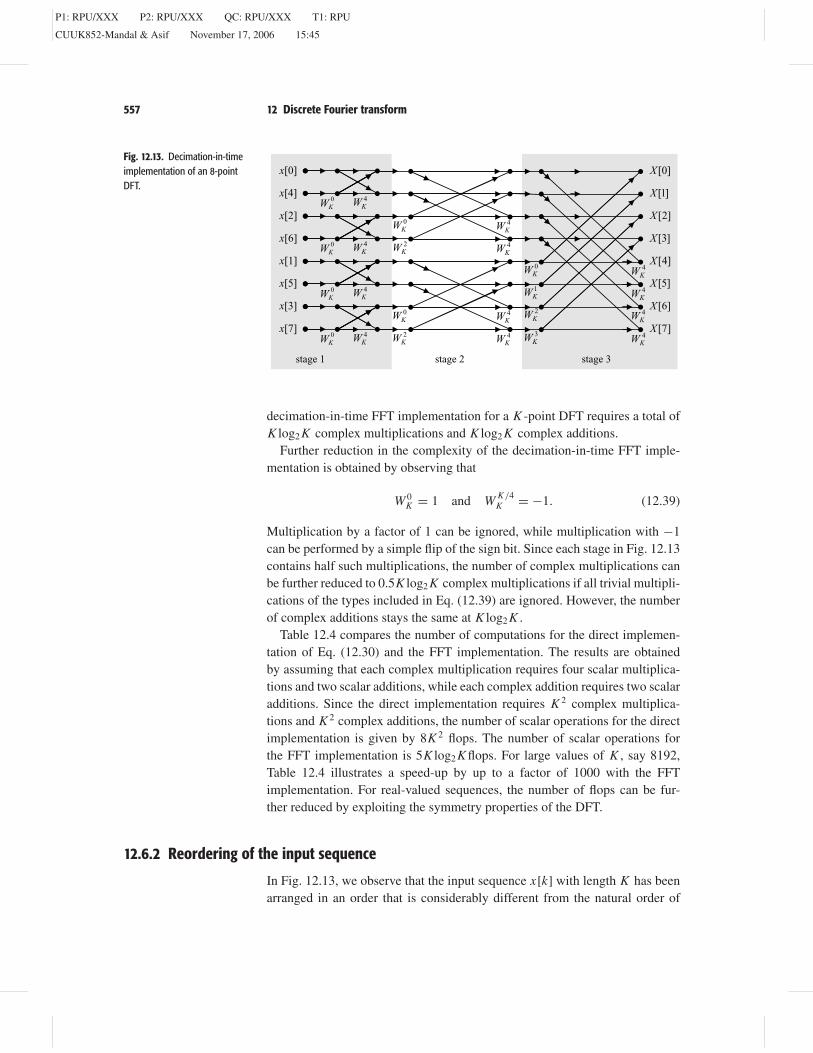
Fig. 12.13. Decimation-in-timeimplementation of an 8-pointDFT.

decimation-in-time FFT implementation for a K -point DFT requires a total ofK log2 K complex multiplications and K log2 K complex additions.

Further reduction in the complexity of the decimation-in-time FFT imple-mentation is obtained by observing that

W 0K = 1 and W K/4

K = −1. (12.39)

Multiplication by a factor of 1 can be ignored, while multiplication with −1can be performed by a simple flip of the sign bit. Since each stage in Fig. 12.13contains half such multiplications, the number of complex multiplications canbe further reduced to 0.5K log2 K complex multiplications if all trivial multipli-cations of the types included in Eq. (12.39) are ignored. However, the numberof complex additions stays the same at K log2 K .

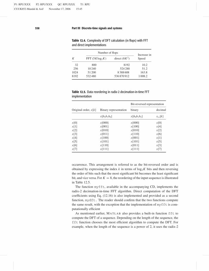
Table 12.4 compares the number of computations for the direct implemen-tation of Eq. (12.30) and the FFT implementation. The results are obtainedby assuming that each complex multiplication requires four scalar multiplica-tions and two scalar additions, while each complex addition requires two scalaradditions. Since the direct implementation requires K 2 complex multiplica-tions and K 2 complex additions, the number of scalar operations for the directimplementation is given by 8K 2 flops. The number of scalar operations forthe FFT implementation is 5K log2 K flops. For large values of K , say 8192,Table 12.4 illustrates a speed-up by up to a factor of 1000 with the FFTimplementation. For real-valued sequences, the number of flops can be fur-ther reduced by exploiting the symmetry properties of the DFT.

12.6.2 Reordering of the input sequence

In Fig. 12.13, we observe that the input sequence x[k] with length K has beenarranged in an order that is considerably different from the natural order of




Table 12.4. Complexity of DFT calculation (in flops) with FFTand direct implementations

Number of flopsIncrease in

K FFT (5K log2 K ) direct (8K 2) Speed

32 800 8192 10.2256 10 240 524 288 51.2

1024 51 200 8 388 608 163.88192 532 480 536 870 912 1 008.2

Table 12.5. Data reordering in radix-2 decimation-in-time FFTimplementation

Bit-reversed representation

Original order, x[k] Binary representation binary decimal

x[b2b1b0] x[b0b1b2] xre[k]

x[0] x[000] x[000] x[0]x[1] x[001] x[100] x[4]x[2] x[010] x[010] x[2]x[3] x[011] x[110] x[6]x[4] x[100] x[001] x[1]x[5] x[101] x[101] x[5]x[6] x[110] x[011] x[3]x[7] x[111] x[111] x[7]

occurrence. This arrangement is referred to as the bit-reversed order and isobtained by expressing the index k in terms of log2 K bits and then reversingthe order of bits such that the most significant bit becomes the least significantbit, and vice versa. For K = 8, the reordering of the input sequence is illustratedin Table 12.5.

The function myfft, available in the accompanying CD, implements theradix-2 decimation-in-time FFT algorithm. Direct computation of the DFTcoefficients using Eq. (12.16) is also implemented and provided as a secondfunction, mydft. The reader should confirm that the two functions computethe same result, with the exception that the implementation of myfft is com-putationally efficient

As mentioned earlier, M A T L A B also provides a built-in function fft tocompute the DFT of a sequence. Depending on the length of the sequence, thefft function chooses the most efficient algorithm to compute the DFT. Forexample, when the length of the sequence is a power of 2, it uses the radix-2




algorithm. On the other hand, if the length is a prime number that cannot befactorized, it uses the direct method based on Eq. (12.16).

12.7 Summary

This chapter introduces the discrete Fourier transform (DFT) for time-limitedsequences as an extension of the DTFT where the DTFT frequency is dis-cretized to a finite set of values = 2r/M , for 0 ≤ r ≤ (M − 1). The M-pointDFT pair for a causal, aperiodic sequence x[k] of length N is defined as follows:

DFT synthesis equation x[k] = 1

M

M−1∑r=0

X [r ]e j(2kr/M) for 0 ≤ k ≤ (N − 1);

DFT analysis equation X [r ] =N−1∑k=0

x[k]e−j(2kr/M) for 0 ≤ r ≤ (M − 1).

For M = N , Section 12.2 implements the synthesis and analysis equations ofthe DFT in the matrix-vector format as follows:

DFT synthesis equation x = FX;

DFT analysis equation X = F−1x,

where F is defined as the DFT matrix given by

F =

1 1 1 · · · 11 e−j(2/N ) e−j(4/N ) · · · e−j(2(N−1)/N )

1 e−j(4/N ) e−j(8/N ) · · · e−j(4(N−1)/N )

......

.... . .

...1 e−j(2(N−1)/N ) e−j(4(N−1)/N ) · · · e−j(2(N−1)(N−1)/N )

.

The columns (or equivalently the rows) of the DFT matrix define the basisfunctions for the DFT.

Section 12.3 used the M-point DFT X [r ] to estimate the CTFT spectrumX () of an aperiodic signal x(t) using the following relationship:

X (r ) ≈ MT1

NX2[r ],

where T1 is the sampling interval used to discretize x(t), r are the CTFTfrequencies that are given by 2r/(M × T1) for −0.5(M−1) ≤ r ≤ 0.5(M−1),and N is the number of samples obtained from the CT signal. Similarly, theDFT X [r ] can be used to determine the DTFT X () of a time-limited sequencex[k] of length Nas

X2(r ) = N

MX2[r ]

at discrete frequencies r = 2r/M , for 0 ≤ r ≤ (M− 1).




Section 12.4 covered the following properties of the DFT.

(1) The periodicity property states that the M-point DFT of a sequence isperiodic with period M .

(2) The orthogonality property states that the basis functions of the DFTs areorthogonal to each other.

(3) The linearity property states that the overall DFT of a linear combinationof DT sequences is given by the same linear combination of the individualDFTs.

(4) The Hermitian symmetry property states that the DFT of a real-valuedsequence is Hermitian. In other words, the real component of the DFTof a real-valued sequence is even, while the imaginary component isodd.

(5) The time-shifting property states that shifting a sequence in the time domaintowards the right-hand side by an integer constant m is equivalent to mul-tiplying the DFT of the original sequence by a complex exponential givenby exp(−j2m/M). Similarly, shifting towards the left-hand side by aninteger m is equivalent to multiplying the DTFT of the original sequenceby a complex exponential given by exp(j2m/M).

(6) The time-convolution property states that the periodic convolution of twoDT sequences is equivalent to the multiplication of the individual DFTs ofthe two sequences in the frequency domain.

(7) Parseval’s theorem states that the energy of a DT sequence is preserved inthe DFT domain.

Section 12.5 used the convolution property to derive alternative procedures forcomputing the convolution sum. These procedures are computationally opti-mal and use fast Fourier transform (FFT) implementations for the DFT toprovide considerable savings over the direct implementation of the convolutionsum.

Section 12.6 covers the decimation-in-time FFT implementation of the DFT.In deriving the FFT algorithm, we assume that the length N of the sequenceequals the number M of samples in the DFT, i.e. N = M = K . We showedthat if K is a power of 2, then the FFT implementations have a computationalcomplexity of O(K log2 K ).

Problems

12.1 Determine analytically the DFT of the following time sequences, withlength 0 ≤ k ≤ (N − 1):

(i) x[k] =

1 k = 0, 3

0 k = 1, 2with length N = 4;




(ii) x[k] =

1 k even

−1 k oddwith length N = 8;

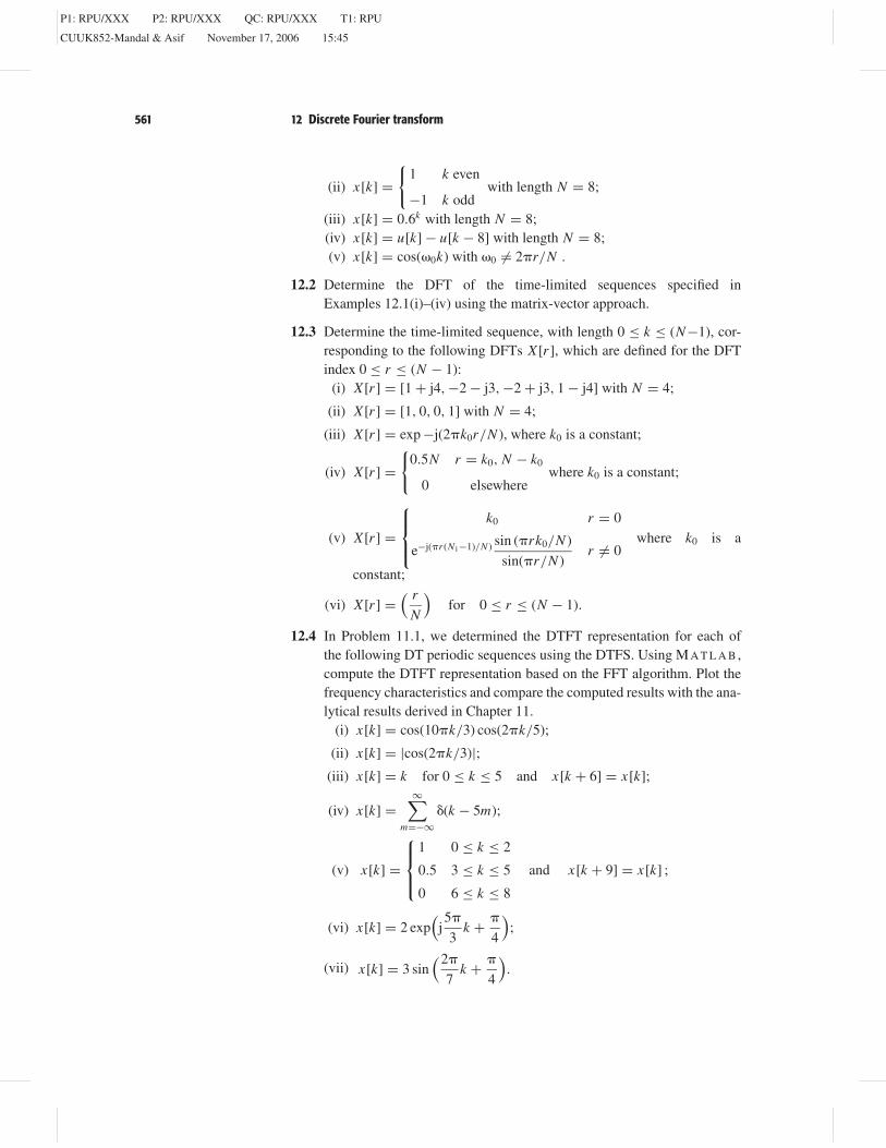
(iii) x[k] = 0.6k with length N = 8;(iv) x[k] = u[k] − u[k − 8] with length N = 8;(v) x[k] = cos(0k) with 0 = 2r/N .

12.2 Determine the DFT of the time-limited sequences specified inExamples 12.1(i)–(iv) using the matrix-vector approach.

12.3 Determine the time-limited sequence, with length 0 ≤ k ≤ (N−1), cor-responding to the following DFTs X [r ], which are defined for the DFTindex 0 ≤ r ≤ (N − 1):

(i) X [r ] = [1 + j4, −2 − j3, −2 + j3, 1 − j4] with N = 4;

(ii) X [r ] = [1, 0, 0, 1] with N = 4;

(iii) X [r ] = exp −j(2k0r/N ), where k0 is a constant;

(iv) X [r ] =

0.5N r = k0, N − k0

0 elsewherewhere k0 is a constant;

(v) X [r ] =

k0 r = 0

e−j(r (N1−1)/N ) sin (rk0/N )

sin(r/N )r = 0

where k0 is a

constant;

(vi) X [r ] =( r

N

)for 0 ≤ r ≤ (N − 1).

12.4 In Problem 11.1, we determined the DTFT representation for each ofthe following DT periodic sequences using the DTFS. Using M A T L A B ,compute the DTFT representation based on the FFT algorithm. Plot thefrequency characteristics and compare the computed results with the ana-lytical results derived in Chapter 11.

(i) x[k] = cos(10k/3) cos(2k/5);

(ii) x[k] = |cos(2k/3)|;(iii) x[k] = k for 0 ≤ k ≤ 5 and x[k + 6] = x[k];

(iv) x[k] =∞∑

m=−∞(k − 5m);

(v) x[k] =

1 0 ≤ k ≤ 2

0.5 3 ≤ k ≤ 5

0 6 ≤ k ≤ 8

and x[k + 9] = x[k] ;

(vi) x[k] = 2 exp(

j5

3k +

4

);

(vii) x[k] = 3 sin(2

7k +

4

).




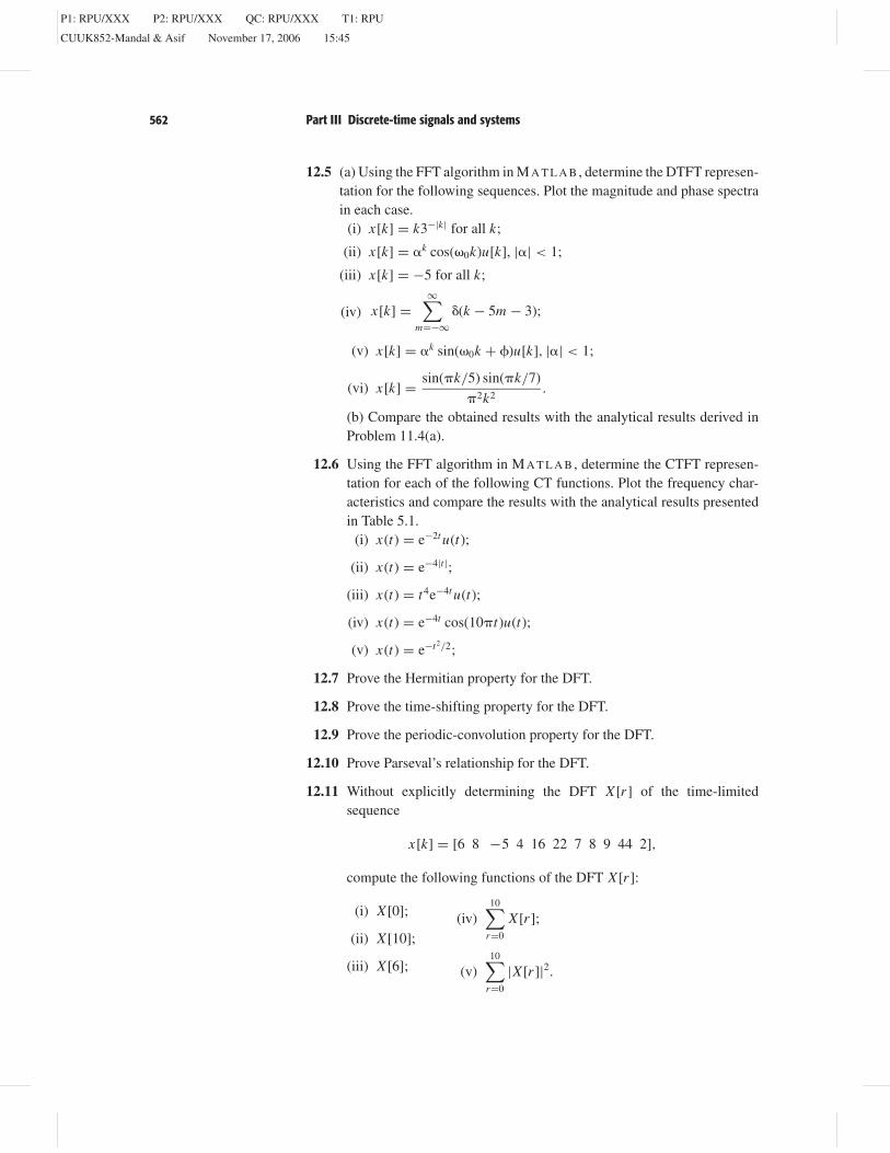
12.5 (a) Using the FFT algorithm in M A T L A B , determine the DTFT represen-tation for the following sequences. Plot the magnitude and phase spectrain each case.

(i) x[k] = k3−|k| for all k;

(ii) x[k] = k cos(0k)u[k], || < 1;

(iii) x[k] = −5 for all k;

(iv) x[k] =∞∑

m=−∞(k − 5m − 3);

(v) x[k] = k sin(0k + )u[k], || < 1;

(vi) x[k] = sin(k/5) sin(k/7)

2k2.

(b) Compare the obtained results with the analytical results derived inProblem 11.4(a).

12.6 Using the FFT algorithm in M A T L A B , determine the CTFT represen-tation for each of the following CT functions. Plot the frequency char-acteristics and compare the results with the analytical results presentedin Table 5.1.

(i) x(t) = e−2t u(t);

(ii) x(t) = e−4|t |;

(iii) x(t) = t4e−4t u(t);

(iv) x(t) = e−4t cos(10t)u(t);

(v) x(t) = e−t2/2;

12.7 Prove the Hermitian property for the DFT.

12.8 Prove the time-shifting property for the DFT.

12.9 Prove the periodic-convolution property for the DFT.

12.10 Prove Parseval’s relationship for the DFT.

12.11 Without explicitly determining the DFT X [r ] of the time-limitedsequence

x[k] = [6 8 −5 4 16 22 7 8 9 44 2],

compute the following functions of the DFT X [r ]:

(i) X [0];

(ii) X [10];

(iii) X [6];

(iv)10∑

r=0

X [r ];

(v)10∑

r=0

|X [r ]|2.




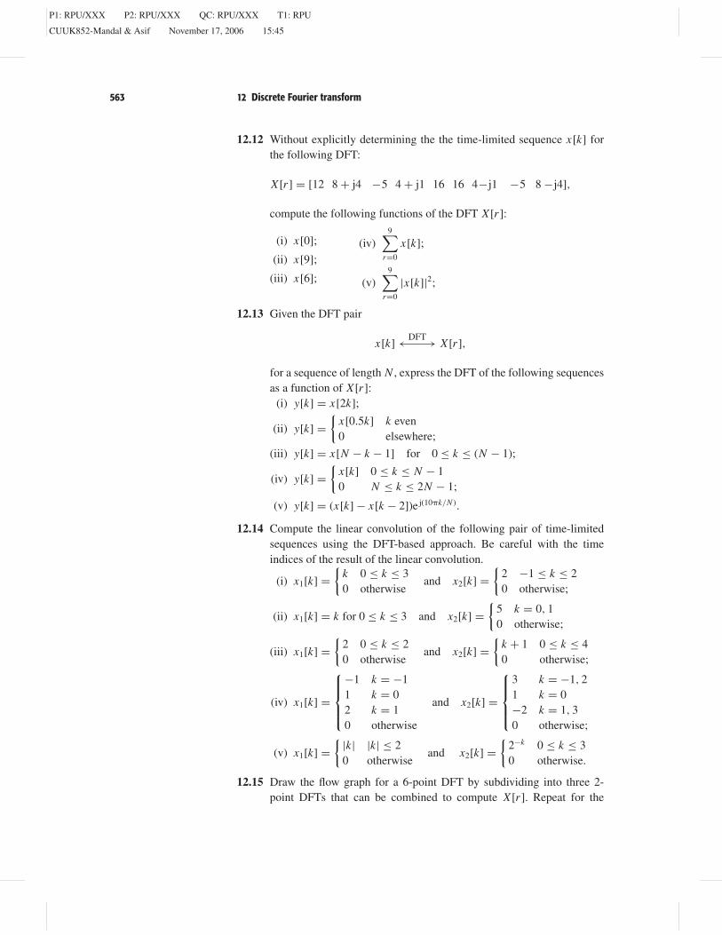
12.12 Without explicitly determining the the time-limited sequence x[k] forthe following DFT:

X [r ] = [12 8 + j4 −5 4 + j1 16 16 4−j1 −5 8 −j4],

compute the following functions of the DFT X [r ]:

(i) x[0];

(ii) x[9];

(iii) x[6];

(iv)9∑

r=0

x[k];

(v)9∑

r=0

|x[k]|2;

12.13 Given the DFT pair

x[k]DFT←−−→ X [r ],

for a sequence of length N , express the DFT of the following sequencesas a function of X [r ]:

(i) y[k] = x[2k];

(ii) y[k] =

x[0.5k] k even0 elsewhere;

(iii) y[k] = x[N − k − 1] for 0 ≤ k ≤ (N − 1);

(iv) y[k] =

x[k] 0 ≤ k ≤ N − 10 N ≤ k ≤ 2N − 1;

(v) y[k] = (x[k] − x[k − 2])e j(10k/N ).

12.14 Compute the linear convolution of the following pair of time-limitedsequences using the DFT-based approach. Be careful with the timeindices of the result of the linear convolution.

(i) x1[k] =

k 0 ≤ k ≤ 30 otherwise

and x2[k] =

2 −1 ≤ k ≤ 20 otherwise;

(ii) x1[k] = k for 0 ≤ k ≤ 3 and x2[k] =

5 k = 0, 10 otherwise;

(iii) x1[k] =

2 0 ≤ k ≤ 20 otherwise

and x2[k] =

k + 1 0 ≤ k ≤ 40 otherwise;

(iv) x1[k] =

−1 k = −11 k = 02 k = 10 otherwise

and x2[k] =

3 k = −1, 21 k = 0−2 k = 1, 30 otherwise;

(v) x1[k] = |k| |k| ≤ 2

0 otherwiseand x2[k] =

2−k 0 ≤ k ≤ 30 otherwise.

12.15 Draw the flow graph for a 6-point DFT by subdividing into three 2-point DFTs that can be combined to compute X [r ]. Repeat for the




subdivision of two 3-point DFTs. Which one provides more compu-tational savings?

12.16 Draw a flow graph for a 10-point decimation-in-time FFT algorithmusing two DFTs of size 5 in the first stage of the flow graph and five DFTsof size 2 in the second stage. Compare the computational complexity ofthe algorithm with the direct approach based on the definition.

12.17 Assume that K = 33. Draw the flow graph for a K -point decimation-in-time FFT algorithm consisting of three stages by using radix-3 asthe basic building block. Compare the computational complexity of thealgorithm with the direct approach based on the definition.

4421 chapter 12_-_discrete_fourier_transform (2)

Documents

discretetime fourier

digital conversion

discrete fourier

continuoustime fourier

digital computations

digital devices

ct signal xt

discretetime signals