4. MA(2) +drift: yt = µ + εt + θ1εt−1 + θ2εt−2

Mean:

yt = µ + θ(L)εt,

where θ(L) = 1 + θ1L + θ2L2.

Therefore,

E(yt) = µ + θ(L)E(εt) = µ

61

Example: MA(q) Model: yt = εt + θ1εt−1 + θ2εt−2 + · · · + θqεt−q

1. Mean of MA(q) Process:

E(yt) = E(εt + θ1εt−1 + θ2εt−2 + · · · + θqεt−q) = 0

2. Autocovariance Function of MA(q) Process:

γ(τ) =

σ2ε (θ0θτ + θ1θτ+1 + · · · + θq−τθq) = σ2

ε

q−τ∑i=0

θiθτ+i, τ = 1, 2, · · · , q,

0, τ = q + 1, q + 2, · · · ,

where θ0 = 1.

62

3. MA( q) process is stationary.

4. MA(q) +drift: yt = µ + εt + θ1εt−1 + θ2εt−2 + · · · + θqεt−q

Mean:

yt = µ + θ(L)εt,

where θ(L) = 1 + θ1L + θ2L2 + · · · + θqLq.

Therefore, we have:

E(yt) = µ + θ(L)E(εt) = µ.

63

1.4 ARMA Model

ARMA (Autoregressive Moving Average，自己回帰移動平均) Process

1. ARMA(p, q)

yt = φ1yt−1 + φ2yt−2 + · · · + φpyt−p + εt + θ1εt−1 + θ2εt−2 + · · · + θqεt−q,

which is rewritten as:

φ(L)yt = θ(L)εt,

where φ(L) = 1−φ1L−φ2L2− · · · −φpLp and θ(L) = 1+θ1L+θ2L2+ · · · +θqLq.

64

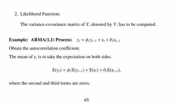
2. Likelihood Function:

The variance-covariance matrix of Y , denoted by V , has to be computed.

Example: ARMA(1,1) Process: yt = φ1yt−1 + εt + θ1εt−1

Obtain the autocorrelation coefficient.

The mean of yt is to take the expectation on both sides.

E(yt) = φ1E(yt−1) + E(εt) + θ1E(εt−1),

where the second and third terms are zeros.

65

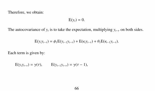
Therefore, we obtain:

E(yt) = 0.

The autocovariance of yt is to take the expectation, multiplying yt−τ on both sides.

E(ytyt−τ) = φ1E(yt−1yt−τ) + E(εtyt−τ) + θ1E(εt−1yt−τ).

Each term is given by:

E(ytyt−τ) = γ(τ), E(yt−1yt−τ) = γ(τ − 1),

66

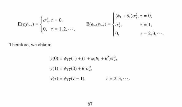
E(εtyt−τ) =

σ2ε , τ = 0,

0, τ = 1, 2, · · · ,E(εt−1yt−τ) =

(φ1 + θ1)σ2

ε , τ = 0,

σ2ε , τ = 1,

0, τ = 2, 3, · · · .

Therefore, we obtain;

γ(0) = φ1γ(1) + (1 + φ1θ1 + θ21)σ2

ε ,

γ(1) = φ1γ(0) + θ1σ2ε ,

γ(τ) = φ1γ(τ − 1), τ = 2, 3, · · · .

67

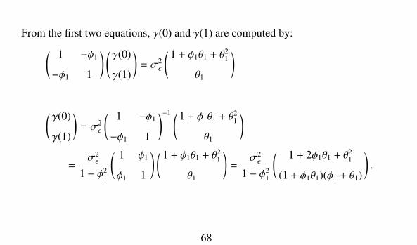
From the first two equations, γ(0) and γ(1) are computed by:( 1 −φ1

−φ1 1

) (γ(0)

γ(1)

)= σ2

ε

( 1 + φ1θ1 + θ21

θ1

)

(γ(0)

γ(1)

)= σ2

ε

( 1 −φ1

−φ1 1

)−1 ( 1 + φ1θ1 + θ21

θ1

)

=σ2ε

1 − φ21

( 1 φ1

φ1 1

) ( 1 + φ1θ1 + θ21

θ1

)=σ2ε

1 − φ21

( 1 + 2φ1θ1 + θ21

(1 + φ1θ1)(φ1 + θ1)

).

68

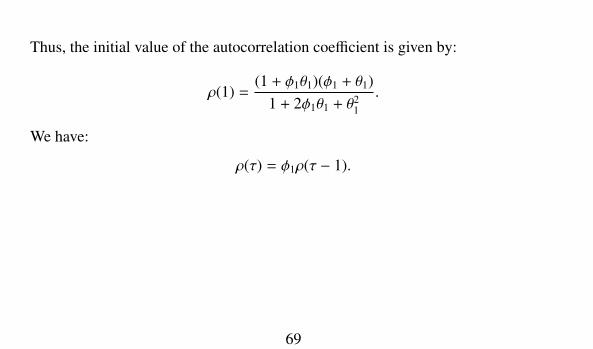
Thus, the initial value of the autocorrelation coefficient is given by:

ρ(1) =(1 + φ1θ1)(φ1 + θ1)

1 + 2φ1θ1 + θ21

.

We have:

ρ(τ) = φ1ρ(τ − 1).

69

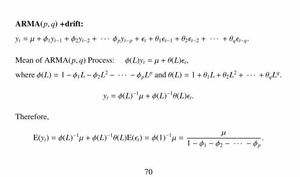
ARMA(p, q) +drift:

yt = µ + φ1yt−1 + φ2yt−2 + · · · φpyt−p + εt + θ1εt−1 + θ2εt−2 + · · · + θqεt−q.

Mean of ARMA(p, q) Process: φ(L)yt = µ + θ(L)εt,

where φ(L) = 1− φ1L− φ2L2 − · · · − φpLp and θ(L) = 1+ θ1L+ θ2L2 + · · · + θqLq.

yt = φ(L)−1µ + φ(L)−1θ(L)εt.

Therefore,

E(yt) = φ(L)−1µ + φ(L)−1θ(L)E(εt) = φ(1)−1µ =µ

1 − φ1 − φ2 − · · · − φp.

70

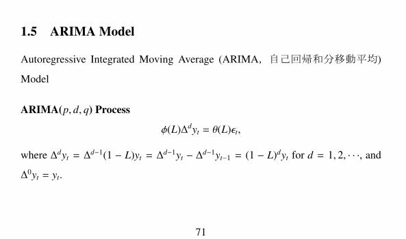
1.5 ARIMA Model

Autoregressive Integrated Moving Average (ARIMA，自己回帰和分移動平均)

Model

ARIMA(p, d, q) Process

φ(L)∆dyt = θ(L)εt,

where ∆dyt = ∆d−1(1 − L)yt = ∆

d−1yt − ∆d−1yt−1 = (1 − L)dyt for d = 1, 2, · · ·, and

∆0yt = yt.

71

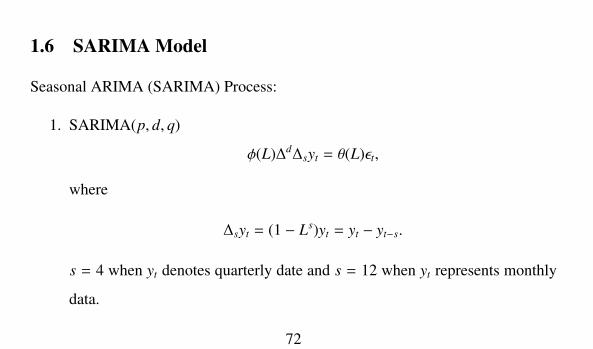
1.6 SARIMA Model

Seasonal ARIMA (SARIMA) Process:

1. SARIMA(p, d, q)

φ(L)∆d∆syt = θ(L)εt,

where

∆syt = (1 − Ls)yt = yt − yt−s.

s = 4 when yt denotes quarterly date and s = 12 when yt represents monthly

data.

72

1.7 Optimal Prediction

1. AR(p) Process: yt = φ1yt−1 + · · · + φpyt−p + εt

(a) Define:

E(yt+k|Yt) = yt+k|t,

where Yt denotes all the information available at time t.

Taking the conditional expectation of yt+k = φ1yt+k−1+ · · · +φpyt+k−p+εt+k

on both sides,

yt+k|t = φ1yt+k−1|t + · · · + φpyt+k−p|t,

73

where ys|t = ys for s ≤ t.

(b) Optimal prediction is given by solving the above differential equation.

2. MA(q) Process: yt = εt + θ1εt−1 + · · · + θqεt−q

(a) Let εT , εT−1, · · ·, ε1 be the estimated errors.

(b) yt+k = εt+k + θ1εt+k−1 + · · · + θqεt+k−q

(c) Therefore,

yt+k|t = εt+k|t + θ1εt+k−1|t + · · · + θqεt+k−q|t,

where εs|t = 0 for s > t and εs|t = εs for s ≤ t.

74

3. ARMA(p, q) Process: yt = φ1yt−1 + · · · + φpyt−p + εt + θ1εt−1 + · · · + θqεt−q

(a) yt+k = φ1yt+k−1 + · · · + φpyt+k−p + εt+k + θ1εt+k−1 + · · · + θqεt+k−q

(b) Optimal prediction is:

yt+k|t = φ1yt+k−1|t + · · · + φpyt+k−p|t + εt+k|t + θ1εt+k−1|t + · · · + θqεt+k−q|t,

where ys|t = ys and εs|t = εs for s ≤ t, and εs|t = 0 for s > t.

75

1.8 Identification

1. Based on AIC or SBIC given d, s, we obtain p, q.

(a) AIC (Akaike’s Information Criterion)

AIC = −2 log(likelihood) + 2k,

where k = p + q, which is the number of parameters estimated.

(b) SBIC (Shwarz’s Bayesian Information Criterion)

SBIC = −2 log(likelihood) + k log T,

76

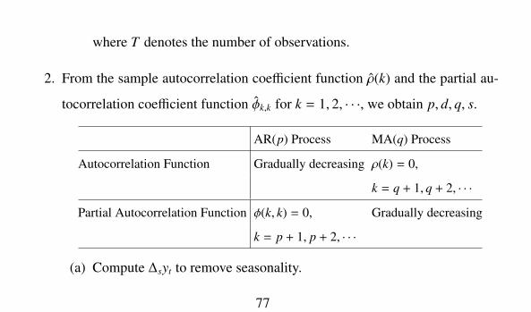
where T denotes the number of observations.

2. From the sample autocorrelation coefficient function ρ(k) and the partial au-

tocorrelation coefficient function φk,k for k = 1, 2, · · ·, we obtain p, d, q, s.

AR(p) Process MA(q) Process

Autocorrelation Function Gradually decreasing ρ(k) = 0,

k = q + 1, q + 2, · · ·

Partial Autocorrelation Function φ(k, k) = 0, Gradually decreasing

k = p + 1, p + 2, · · ·

(a) Compute ∆syt to remove seasonality.

77

Compute the autocovariance functions of ∆syt.

If the autocovariance functions have period s, we take (1 − Ls), again.

(b) Determine the order of difference.

Compute the partial autocovariance functions every time.

If the autocovariance functions decrease as τ is large, go to the next step.

(c) Determine the order of AR terms (i.e., p).

Compute the partial autocovariance functions every time.

The partial autocovariance functions are close to zero after some τ, go

to the next step.

78

(d) Determine the order of MA terms (i.e., q).

Compute the autocovariance functions every time.

If the autocovariance functions are randomly around zero, end of the

procedure.

79

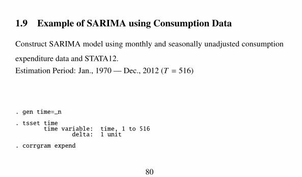
1.9 Example of SARIMA using Consumption Data

Construct SARIMA model using monthly and seasonally unadjusted consumption

expenditure data and STATA12.Estimation Period: Jan., 1970 — Dec., 2012 (T = 516)

. gen time=_n

. tsset timetime variable: time, 1 to 516

delta: 1 unit

. corrgram expend

80

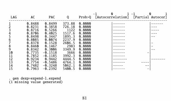
-1 0 1 -1 0 1LAG AC PAC Q Prob>Q [Autocorrelation] [Partial Autocor]-------------------------------------------------------------------------------1 0.8488 0.8499 373.88 0.0000 |------ |------2 0.8231 0.3858 726.18 0.0000 |------ |---3 0.8716 0.5266 1122 0.0000 |------ |----4 0.8706 0.4025 1517.6 0.0000 |------ |---5 0.8498 0.3447 1895.3 0.0000 |------ |--6 0.8085 0.0074 2237.9 0.0000 |------ |7 0.8378 0.1528 2606.5 0.0000 |------ |-8 0.8460 0.1467 2983 0.0000 |------ |-9 0.8342 0.3006 3349.9 0.0000 |------ |--10 0.7735 -0.1518 3666 0.0000 |------ -|11 0.7852 -0.1185 3992.3 0.0000 |------ |12 0.9234 0.9442 4444.5 0.0000 |------- |-------13 0.7754 -0.5486 4764.1 0.0000 |------ ----|14 0.7482 -0.3248 5062.1 0.0000 |----- --|15 0.7963 -0.2392 5400.5 0.0000 |------ -|

. gen dexp=expend-l.expend(1 missing value generated)

81

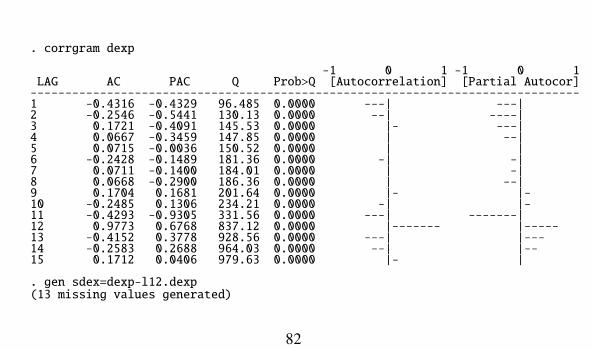
. corrgram dexp

-1 0 1 -1 0 1LAG AC PAC Q Prob>Q [Autocorrelation] [Partial Autocor]-------------------------------------------------------------------------------1 -0.4316 -0.4329 96.485 0.0000 ---| ---|2 -0.2546 -0.5441 130.13 0.0000 --| ----|3 0.1721 -0.4091 145.53 0.0000 |- ---|4 0.0667 -0.3459 147.85 0.0000 | --|5 0.0715 -0.0036 150.52 0.0000 | |6 -0.2428 -0.1489 181.36 0.0000 -| -|7 0.0711 -0.1400 184.01 0.0000 | -|8 0.0668 -0.2900 186.36 0.0000 | --|9 0.1704 0.1681 201.64 0.0000 |- |-10 -0.2485 0.1306 234.21 0.0000 -| |-11 -0.4293 -0.9305 331.56 0.0000 ---| -------|12 0.9773 0.6768 837.12 0.0000 |------- |-----13 -0.4152 0.3778 928.56 0.0000 ---| |---14 -0.2583 0.2688 964.03 0.0000 --| |--15 0.1712 0.0406 979.63 0.0000 |- |

. gen sdex=dexp-l12.dexp(13 missing values generated)

82

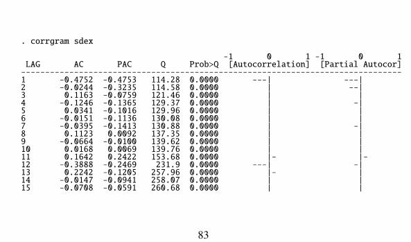
. corrgram sdex

-1 0 1 -1 0 1LAG AC PAC Q Prob>Q [Autocorrelation] [Partial Autocor]-------------------------------------------------------------------------------1 -0.4752 -0.4753 114.28 0.0000 ---| ---|2 -0.0244 -0.3235 114.58 0.0000 | --|3 0.1163 -0.0759 121.46 0.0000 | |4 -0.1246 -0.1365 129.37 0.0000 | -|5 0.0341 -0.1016 129.96 0.0000 | |6 -0.0151 -0.1136 130.08 0.0000 | |7 -0.0395 -0.1413 130.88 0.0000 | -|8 0.1123 0.0092 137.35 0.0000 | |9 -0.0664 -0.0100 139.62 0.0000 | |10 0.0168 0.0069 139.76 0.0000 | |11 0.1642 0.2422 153.68 0.0000 |- |-12 -0.3888 -0.2469 231.9 0.0000 ---| -|13 0.2242 -0.1205 257.96 0.0000 |- |14 -0.0147 -0.0941 258.07 0.0000 | |15 -0.0708 -0.0591 260.68 0.0000 | |

83

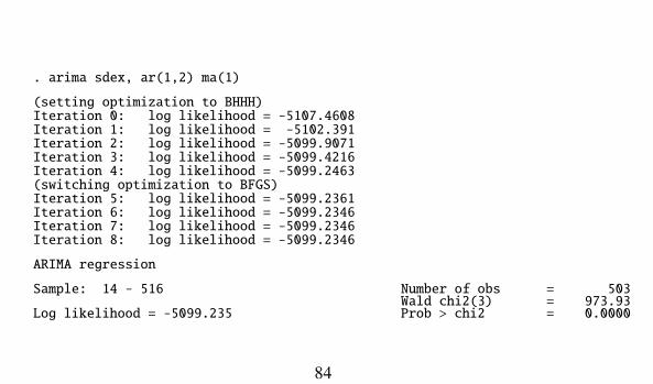
. arima sdex, ar(1,2) ma(1)

(setting optimization to BHHH)Iteration 0: log likelihood = -5107.4608Iteration 1: log likelihood = -5102.391Iteration 2: log likelihood = -5099.9071Iteration 3: log likelihood = -5099.4216Iteration 4: log likelihood = -5099.2463(switching optimization to BFGS)Iteration 5: log likelihood = -5099.2361Iteration 6: log likelihood = -5099.2346Iteration 7: log likelihood = -5099.2346Iteration 8: log likelihood = -5099.2346

ARIMA regression

Sample: 14 - 516 Number of obs = 503Wald chi2(3) = 973.93

Log likelihood = -5099.235 Prob > chi2 = 0.0000

84

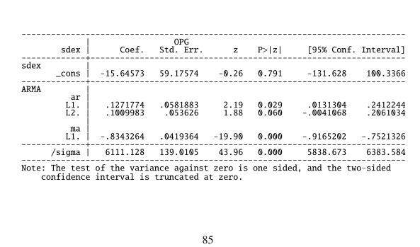
------------------------------------------------------------------------------| OPG

sdex | Coef. Std. Err. z P>|z| [95% Conf. Interval]-------------+----------------------------------------------------------------sdex |

_cons | -15.64573 59.17574 -0.26 0.791 -131.628 100.3366-------------+----------------------------------------------------------------ARMA |

ar |L1. | .1271774 .0581883 2.19 0.029 .0131304 .2412244L2. | .1009983 .053626 1.88 0.060 -.0041068 .2061034

|ma |L1. | -.8343264 .0419364 -19.90 0.000 -.9165202 -.7521326

-------------+----------------------------------------------------------------/sigma | 6111.128 139.0105 43.96 0.000 5838.673 6383.584

------------------------------------------------------------------------------Note: The test of the variance against zero is one sided, and the two-sided

confidence interval is truncated at zero.

85

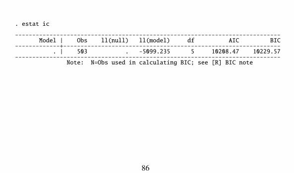
. estat ic

-----------------------------------------------------------------------------Model | Obs ll(null) ll(model) df AIC BIC

-------------+---------------------------------------------------------------. | 503 . -5099.235 5 10208.47 10229.57

-----------------------------------------------------------------------------Note: N=Obs used in calculating BIC; see [R] BIC note

86

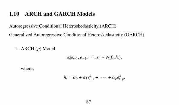
1.10 ARCH and GARCH Models

Autoregressive Conditional Heteroskedasticity (ARCH)

Generalized Autoregressive Conditional Heteroskedasticity (GARCH)

1. ARCH (p) Model

εt|εt−1, εt−2, · · · , ε1 ∼ N(0, ht),

where，

ht = α0 + α1ε2t−1 + · · · + αpε

2t−p.

87

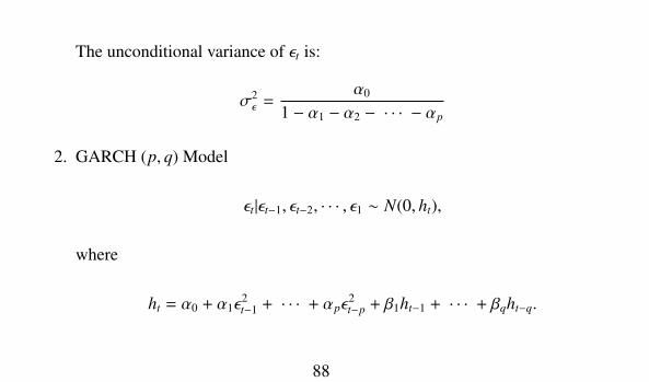
The unconditional variance of εt is:

σ2ε =

α0

1 − α1 − α2 − · · · − αp

2. GARCH (p, q) Model

εt|εt−1, εt−2, · · · , ε1 ∼ N(0, ht),

where

ht = α0 + α1ε2t−1 + · · · + αpε

2t−p + β1ht−1 + · · · + βqht−q.

88

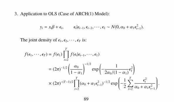
3. Application to OLS (Case of ARCH(1) Model):

yt = xtβ + εt, εt|εt−1, εt−2, · · · , ε1 ∼ N(0, α0 + α1ε2t−1).

The joint density of ε1, ε2, · · · , εT is:

f (ε1, · · · , εT ) = f (ε1)T∏

t=2

f (εt|εt−1, · · · , ε1)

= (2π)−1/2(α0

1 − α1

)−1/2

exp(− 1

2α0/(1 − α1)ε21

)× (2π)−(T−1)/2

T∏t=2

(α0 + α1ε2t−1)−1/2 exp

−12

T∑t=2

ε2tα0 + α1ε

2t−1

.89

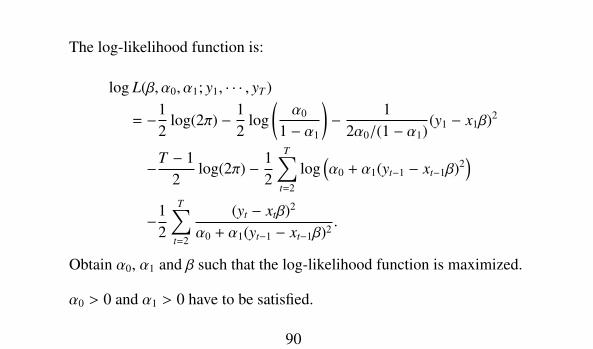
The log-likelihood function is:

log L(β, α0, α1; y1, · · · , yT )

= −12

log(2π) − 12

log(α0

1 − α1

)− 1

2α0/(1 − α1)(y1 − x1β)2

−T − 12

log(2π) − 12

T∑t=2

log(α0 + α1(yt−1 − xt−1β)2

)−1

2

T∑t=2

(yt − xtβ)2

α0 + α1(yt−1 − xt−1β)2 .

Obtain α0, α1 and β such that the log-likelihood function is maximized.

α0 > 0 and α1 > 0 have to be satisfied.

90

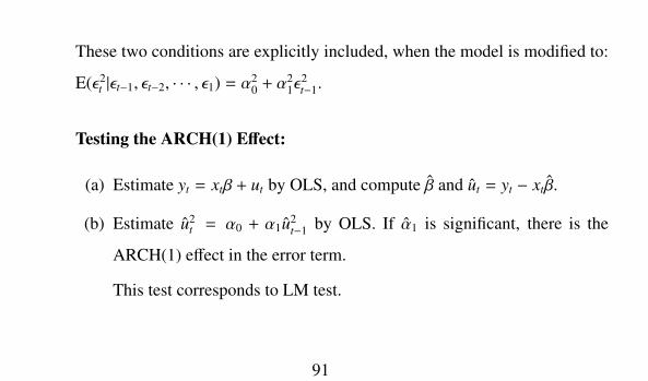
These two conditions are explicitly included, when the model is modified to:

E(ε2t |εt−1, εt−2, · · · , ε1) = α20 + α

21ε

2t−1.

Testing the ARCH(1) Effect:

(a) Estimate yt = xtβ + ut by OLS, and compute β and ut = yt − xtβ.

(b) Estimate u2t = α0 + α1u2

t−1 by OLS. If α1 is significant, there is the

ARCH(1) effect in the error term.

This test corresponds to LM test.

91