36106 managerial decision modeling linear decision...
TRANSCRIPT
36106 Managerial Decision ModelingLinear Decision Models: Part I
Kipp MartinUniversity of Chicago
Booth School of Business
January 16, 2014
1
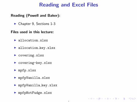
Reading and Excel Files
Reading (Powell and Baker):
I Chapter 9, Sections 1-3
Files used in this lecture:
I allocation.xlsx
I allocation key.xlsx
I covering.xlsx
I covering-key.xlsx
I mpfp.xlsx
I mpfpVanilla.xlsx
I mpfpVanilla key.xlsx
I mpfpHotFudge.xlsx
2
Lecture Outline
Moving From What-If To What’s Best
Resource Allocation Problems
Using Solver
Covering Problems
Cash Flow Matching
Style and Spreadsheet Engineering
3
Moving From What-If To What’s Best
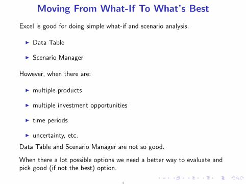
Excel is good for doing simple what-if and scenario analysis.
I Data Table
I Scenario Manager
However, when there are:
I multiple products
I multiple investment opportunities
I time periods
I uncertainty, etc.
Data Table and Scenario Manager are not so good.
When there a lot possible options we need a better way to evaluate andpick good (if not the best) option.
4
Resource Allocation
The resource allocation problem:
I multiple products
I multiple resources
I constraints on the resources
I objective: allocate resources to products in order to maximize profit
We use an unrealistically small problem just to illustrate the process. Ourexample is the Veerman Furniture Company from Section 9.2 of thetextbook.
5
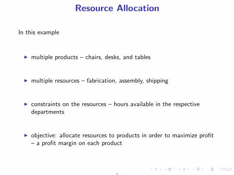
Resource Allocation
In this example
I multiple products – chairs, desks, and tables
I multiple resources – fabrication, assembly, shipping
I constraints on the resources – hours available in the respectivedepartments
I objective: allocate resources to products in order to maximize profit– a profit margin on each product
6
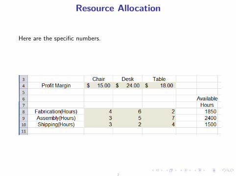
Resource Allocation
Here are the specific numbers.
7
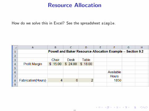
Resource Allocation
Let’s start easy and assume that the fabrication availability is the onlyresource. See workbook allocation.xlsl and spreadsheet simple.
How many chairs, desks, and tables should we make in order to:
I maximize profit
I do not exceed the 1850 hours available in the fabrication department
Let’s give a formal mathematical statement of the problem.
8
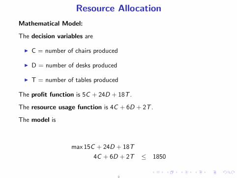
Resource Allocation
Mathematical Model:
The decision variables are
I C = number of chairs produced
I D = number of desks produced
I T = number of tables produced
The profit function is 5C + 24D + 18T .
The resource usage function is 4C + 6D + 2T .
The model is
max 15C + 24D + 18T
4C + 6D + 2T ≤ 1850
9
Resource Allocation
How do we solve this in Excel? See the spreadsheet simple.
10
Resource Allocation
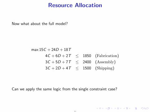
Now what about the full model?
max 15C + 24D + 18T
4C + 6D + 2T ≤ 1850 (Fabrication)
3C + 5D + 7T ≤ 2400 (Assembly)
3C + 2D + 4T ≤ 1500 (Shipping)
Can we apply the same logic from the single constraint case?
11
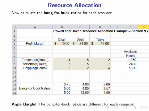
Resource AllocationNow calculate the bang-for-buck ratios for each resource.
Argle Bargle! The bang-for-buck ratios are different for each resource!
12
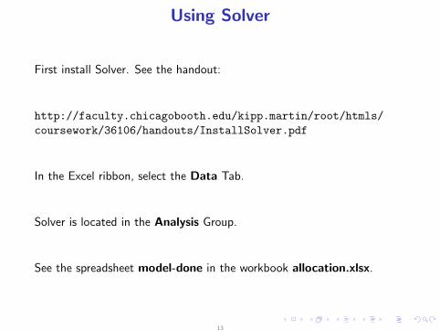
Using Solver
First install Solver. See the handout:
http://faculty.chicagobooth.edu/kipp.martin/root/htmls/
coursework/36106/handouts/InstallSolver.pdf
In the Excel ribbon, select the Data Tab.
Solver is located in the Analysis Group.
See the spreadsheet model-done in the workbook allocation.xlsx.
13
Using Solver
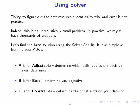
Trying to figure out the best resource allocation by trial and error is notpractical.
Indeed, this is an unrealistically small problem. In practice, we mighthave thousands of products.
Let’s find the best solution using the Solver Add-In. It is as simple aslearning your ABCs.
I A is for Adjustable – determine which cells, you as the decisionmaker, determine
I B is for Best – determine you objective
I C is for Constraints – determine the constraints on your decision
14
Using Solver
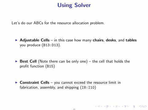
Let’s do our ABCs for the resource allocation problem.
I Adjustable Cells – in this case how many chairs, desks, and tablesyou produce (B13:D13).
I Best Cell (Note there can be only one) – the cell that holds theprofit function (B15)
I Constraint Cells – you cannot exceed the resource limit infabrication, assembly, and shipping (I8:I10)
15
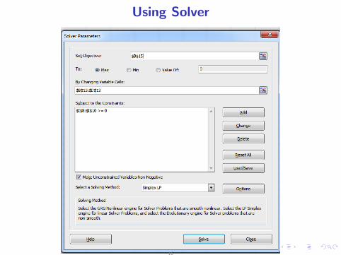
Using Solver
16
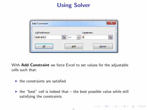
Using Solver
With Add Constraint we force Excel to set values for the adjustablecells such that:
I the constraints are satisfied
I the “best” cell is indeed that – the best possible value while stillsatisfying the constraints.
17
Using Solver
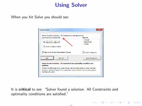
When you hit Solve you should see:
It is critical to see: “Solver found a solution. All Constraints andoptimality conditions are satisfied.”
18
Using Solver
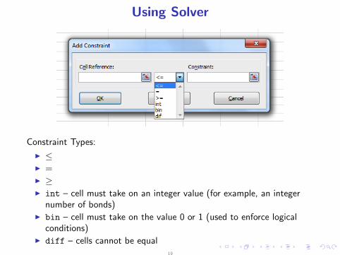
Constraint Types:
I ≤I =I ≥I int – cell must take on an integer value (for example, an integer
number of bonds)I bin – cell must take on the value 0 or 1 (used to enforce logical
conditions)I diff – cells cannot be equal
19
Using Solver
A few other things:
I You can have multiple sets of constraints and they do not need tobe contiguous. Just keep adding them!
I In setting the adjustable cells, the rows do not need to becontiguous, separate by commas.
I You can have only one best cell.
I My color coding for the font
1. Red – constraint cells
2. Blue – adjustable cells
3. Green – best cell
4. Black – parameters
Note: We checked the box for nonnegative variables, what happens if wedon’t?
20
Using Solver
IMPORTANT: There are different ways to setup a solver model.
Method 1: Explicitly calculate a set of slack cells and require the slackto be nonnegative. This was expressed as I8:I10 >= 0. The advantagesare:
I Can see an explicit calculation of the slack.
I Easy to identify the constraints (red cells) in the model.
Method 2: Add constraints that say: “hours used <= hours used.” Thisis expressed as F8:F10 <= H8:H10. (See next slid). The advantages are:
I The spreadsheet is less cluttered.
I The dual or shadow prices have the correct sign. More on this later.
My Advice: develop a style that you feel most comfortable with.
21

Using Solver
22
Resource Alloccation
We assumed we could sell every chair, desk, and table produced.
Modify and solve the problem assuming the following demands.
I the chair demand limit is 360
I the desk demand limit is 300
I the table demand limit is 100
23
Resource Allocation – Pricing
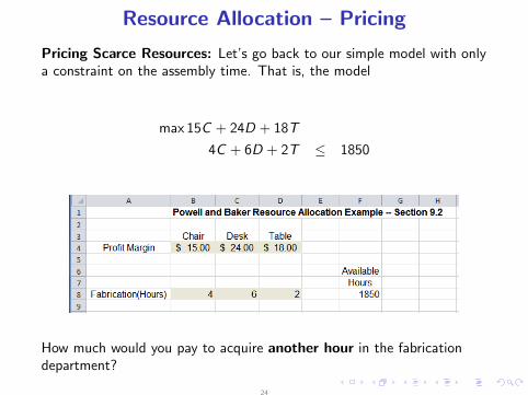
Pricing Scarce Resources: Let’s go back to our simple model with onlya constraint on the assembly time. That is, the model
max 15C + 24D + 18T
4C + 6D + 2T ≤ 1850
How much would you pay to acquire another hour in the fabricationdepartment?
24
Resource Allocation – Pricing
Dual Price: the value of an additional unit of resource. Think of it as amarginal price. Other terms are:
I Shadow Price
I Dual Value
I Lagrange Multiplier
Application: in portfolio optimization the dual price is the slope of theefficient frontier.
Regardless of the number of constraints, solver provides the dual price onall resources.
25
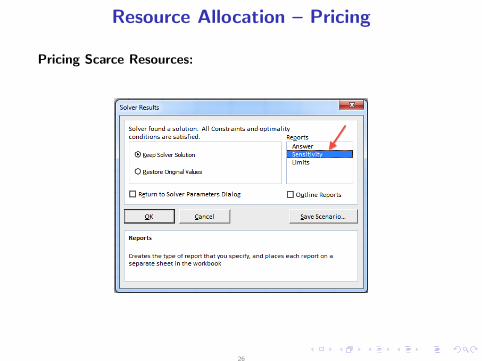
Resource Allocation – Pricing
Pricing Scarce Resources:
26
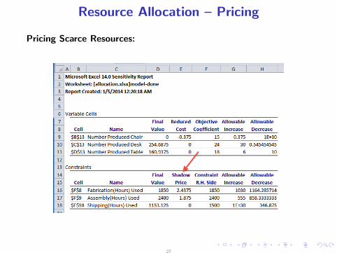
Resource Allocation – Pricing
Pricing Scarce Resources:
27
Covering Problems
Two new modeling tools.
I Excel SUMPRODUCT function
I Range names
28
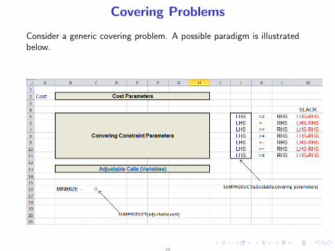
Covering Problems
Consider a generic covering problem. A possible paradigm is illustratedbelow.
29
Covering Problems
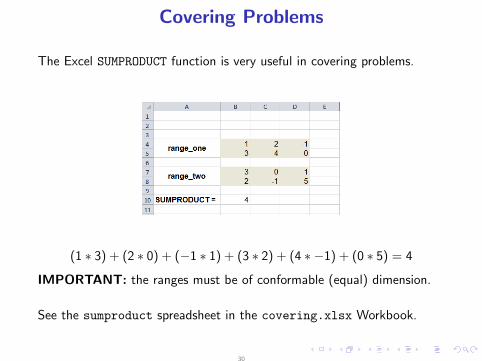
The Excel SUMPRODUCT function is very useful in covering problems.
(1 ∗ 3) + (2 ∗ 0) + (−1 ∗ 1) + (3 ∗ 2) + (4 ∗ −1) + (0 ∗ 5) = 4
IMPORTANT: the ranges must be of conformable (equal) dimension.
See the sumproduct spreadsheet in the covering.xlsx Workbook.
30
Covering Problems
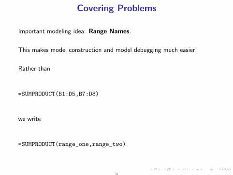
Important modeling idea: Range Names.
This makes model construction and model debugging much easier!
Rather than
=SUMPRODUCT(B1:D5,B7:D8)
we write
=SUMPRODUCT(range_one,range_two)
31
Covering Problems
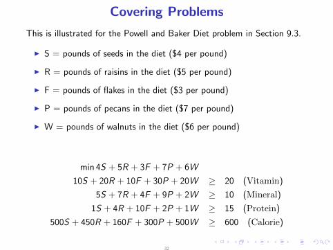
This is illustrated for the Powell and Baker Diet problem in Section 9.3.
I S = pounds of seeds in the diet ($4 per pound)
I R = pounds of raisins in the diet ($5 per pound)
I F = pounds of flakes in the diet ($3 per pound)
I P = pounds of pecans in the diet ($7 per pound)
I W = pounds of walnuts in the diet ($6 per pound)
min 4S + 5R + 3F + 7P + 6W
10S + 20R + 10F + 30P + 20W ≥ 20 (Vitamin)
5S + 7R + 4F + 9P + 2W ≥ 10 (Mineral)
1S + 4R + 10F + 2P + 1W ≥ 15 (Protein)
500S + 450R + 160F + 300P + 500W ≥ 600 (Calorie)
32
Covering Problems
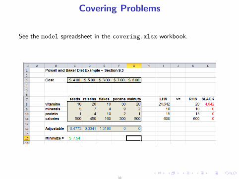
See the model spreadsheet in the covering.xlsx workbook.
33
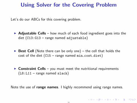
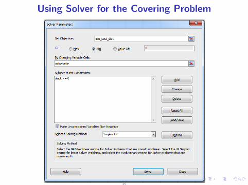
Using Solver for the Covering Problem
Let’s do our ABCs for this covering problem.
I Adjustable Cells – how much of each food ingredient goes into thediet (C13:G13 – range named adjustable)
I Best Cell (Note there can be only one) – the cell that holds thecost of the diet (C15 – range named min cost diet)
I Constraint Cells – you must meet the nutritional requirements(L8:L11 – range named slack)
Note the use of range names. I highly recommend using range names.
34
Using Solver for the Covering Problem
35
Cash Flow Matching
Problem: generate a specified stream of cash flows over a planninghorizon.
I pension fund planning
I law suit settlement
I lottery
Assume you win one million dollars in a state lottery. Option 1 is to takethe one million up front. Option 2 is to receive an annuity of $50,000dollars a year for 30 years. Which is better?
If you pick Option 2 the state will discharge the debt to a bank. Howmuch do they pay the bank?
36
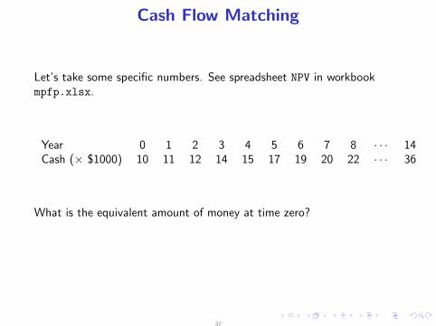
Cash Flow Matching
Let’s take some specific numbers. See spreadsheet NPV in workbookmpfp.xlsx.
Year 0 1 2 3 4 5 6 7 8 · · · 14Cash (× $1000) 10 11 12 14 15 17 19 20 22 · · · 36
What is the equivalent amount of money at time zero?
37
Cash Flow Matching
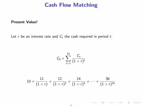
Present Value!
Let r be an interest rate and Ct the cash required in period t.
C0 +14∑t=1
Ct
(1 + r)t
10 +11
(1 + r)+
12
(1 + r)2+
14
(1 + r)3+ · · · +
36
(1 + r)14
38
Cash Flow Matching
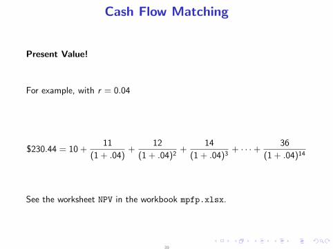
Present Value!
For example, with r = 0.04
$230.44 = 10 +11
(1 + .04)+
12
(1 + .04)2+
14
(1 + .04)3+ · · · +
36
(1 + .04)14
See the worksheet NPV in the workbook mpfp.xlsx.
39
Cash Flow Matching
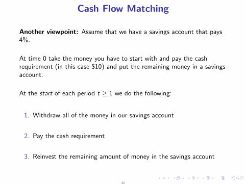
Another viewpoint: Assume that we have a savings account that pays4%.
At time 0 take the money you have to start with and pay the cashrequirement (in this case $10) and put the remaining money in a savingsaccount.
At the start of each period t ≥ 1 we do the following:
1. Withdraw all of the money in our savings account
2. Pay the cash requirement
3. Reinvest the remaining amount of money in the savings account
40
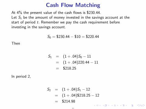
Cash Flow MatchingAt 4% the present value of the cash flows is $230.44.Let St be the amount of money invested in the savings account at thestart of period t. Remember we pay the cash requirement beforeinvesting in the savings account.
S0 = $230.44 − $10 = $220.44
Then
S1 = (1 + .04)S0 − 11
= (1 + .04)220.44 − 11
= $218.25
In period 2,
S2 = (1 + .04)S1 − 12
= (1 + .04)$218.25 − 12
= $214.98
41
Cash Flow Matching
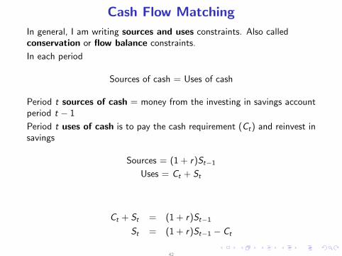
In general, I am writing sources and uses constraints. Also calledconservation or flow balance constraints.
In each period
Sources of cash = Uses of cash
Period t sources of cash = money from the investing in savings accountperiod t − 1
Period t uses of cash is to pay the cash requirement (Ct) and reinvest insavings
Sources = (1 + r)St−1
Uses = Ct + St
Ct + St = (1 + r)St−1
St = (1 + r)St−1 − Ct
42
Cash Flow Matching
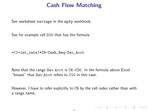
See worksheet savings in the mpfp workbook.
See for example cell D10 that has the formula
=(1+int_rate)*C9-Cash_Req-Sav_Acct
Note that the range Sav Acct is C6:C20. In the formula above Excel“knows” that Sav Acct refers to C10 in this case.
However, I have to refer explicitly to C9 by the cell index rather than witha range name.
43
Cash Flow Matching
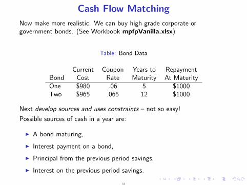
Now make more realistic. We can buy high grade corporate orgovernment bonds. (See Workbook mpfpVanilla.xlsx)
Table: Bond Data
Current Coupon Years to RepaymentBond Cost Rate Maturity At MaturityOne $980 .06 5 $1000Two $965 .065 12 $1000
Next develop sources and uses constraints – not so easy!
Possible sources of cash in a year are:
I A bond maturing,
I Interest payment on a bond,
I Principal from the previous period savings,
I Interest on the previous period savings.
44
Cash Flow Matching
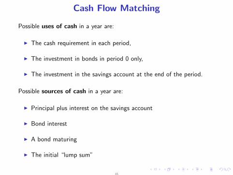
Possible uses of cash in a year are:
I The cash requirement in each period,
I The investment in bonds in period 0 only,
I The investment in the savings account at the end of the period.
Possible sources of cash in a year are:
I Principal plus interest on the savings account
I Bond interest
I A bond maturing
I The initial “lump sum”
45
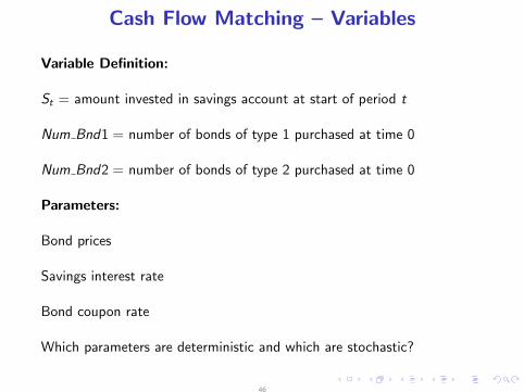
Cash Flow Matching – Variables
Variable Definition:
St = amount invested in savings account at start of period t
Num Bnd1 = number of bonds of type 1 purchased at time 0
Num Bnd2 = number of bonds of type 2 purchased at time 0
Parameters:
Bond prices
Savings interest rate
Bond coupon rate
Which parameters are deterministic and which are stochastic?
46
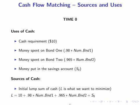
Cash Flow Matching – Sources and Uses
TIME 0
Uses of Cash:
I Cash requirement ($10)
I Money spent on Bond One (.98 ∗ Num Bnd1)
I Money spent on Bond Two (.965 ∗ Num Bnd2)
I Money put in the savings account (S0)
Sources of Cash:
I Initial lump sum of cash (L is what we want to minimize)
L = 10 + .98 ∗ Num Bnd1 + .965 ∗ Num Bnd2 + S0
47
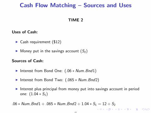
Cash Flow Matching – Sources and Uses
TIME 2
Uses of Cash:
I Cash requirement ($12)
I Money put in the savings account (S2)
Sources of Cash:
I Interest from Bond One: (.06 ∗ Num Bnd1)
I Interest from Bond Two: (.065 ∗ Num Bnd2)
I Interest plus principal from money put into savings account in periodone: (1.04 ∗ S1)
.06 ∗ Num Bnd1 + .065 ∗ Num Bnd2 + 1.04 ∗ S1 = 12 + S2
48
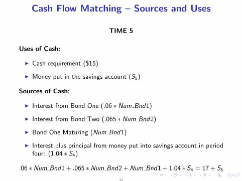
Cash Flow Matching – Sources and Uses
TIME 5
Uses of Cash:
I Cash requirement ($15)
I Money put in the savings account (S5)
Sources of Cash:
I Interest from Bond One (.06 ∗ Num Bnd1)
I Interest from Bond Two (.065 ∗ Num Bnd2)
I Bond One Maturing (Num Bnd1)
I Interest plus principal from money put into savings account in periodfour: (1.04 ∗ S4)
.06 ∗Num Bnd1 + .065 ∗Num Bnd2 + Num Bnd1 + 1.04 ∗ S4 = 17 + S5
49
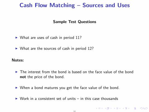
Cash Flow Matching – Sources and Uses
Sample Test Questions
I What are uses of cash in period 11?
I What are the sources of cash in period 12?
Notes:
I The interest from the bond is based on the face value of the bondnot the price of the bond.
I When a bond matures you get the face value of the bond.
I Work in a consistent set of units – in this case thousands
50
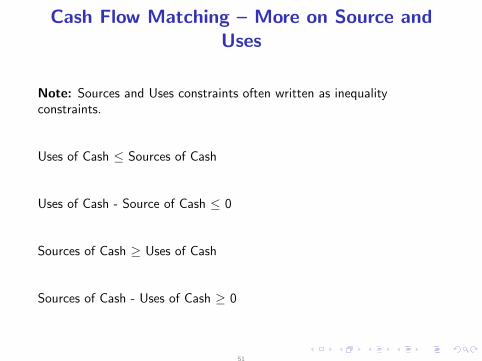
Cash Flow Matching – More on Source andUses
Note: Sources and Uses constraints often written as inequalityconstraints.
Uses of Cash ≤ Sources of Cash
Uses of Cash - Source of Cash ≤ 0
Sources of Cash ≥ Uses of Cash
Sources of Cash - Uses of Cash ≥ 0
51
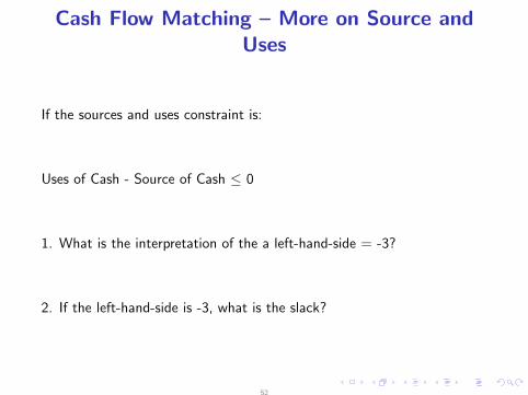
Cash Flow Matching – More on Source andUses
If the sources and uses constraint is:
Uses of Cash - Source of Cash ≤ 0
1. What is the interpretation of the a left-hand-side = -3?
2. If the left-hand-side is -3, what is the slack?
52
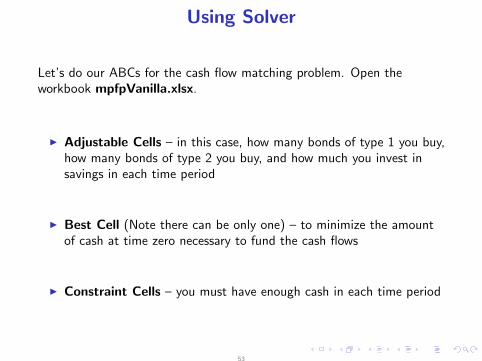
Using Solver
Let’s do our ABCs for the cash flow matching problem. Open theworkbook mpfpVanilla.xlsx.
I Adjustable Cells – in this case, how many bonds of type 1 you buy,how many bonds of type 2 you buy, and how much you invest insavings in each time period
I Best Cell (Note there can be only one) – to minimize the amountof cash at time zero necessary to fund the cash flows
I Constraint Cells – you must have enough cash in each time period
53
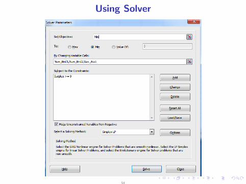
Using Solver
54
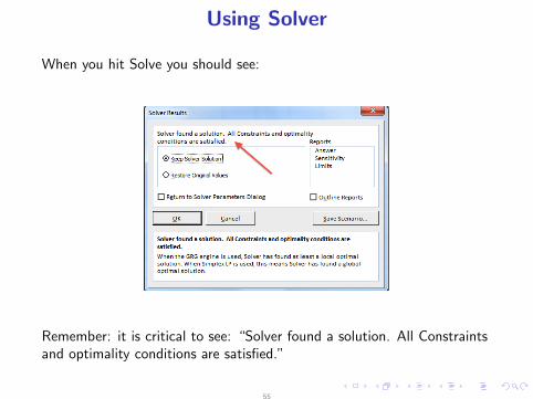
Using Solver
When you hit Solve you should see:
Remember: it is critical to see: “Solver found a solution. All Constraintsand optimality conditions are satisfied.”
55
Cash Flow Matching
Key Takeaways:
I sources and uses constraints
I how to use Solver to find the BEST value
I present value calculation and why it is restrictive
56
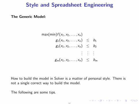
Style and Spreadsheet Engineering
The Generic Model:
max(min)f (x1, x2, . . . , xn)
g1(x1, x2, . . . , xn) ≤ b1
g2(x1, x2, . . . , xn) ≤ b2...
......
gm(x1, x2, . . . , xn) ≤ bm
How to build the model in Solver is a matter of personal style. There isnot a single correct way to build the model.
The following are some tips.
57
Style and Spreadsheet Engineering
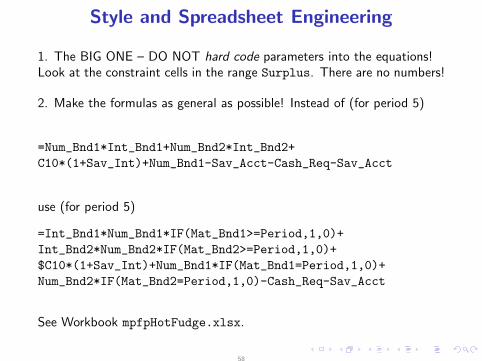
1. The BIG ONE – DO NOT hard code parameters into the equations!Look at the constraint cells in the range Surplus. There are no numbers!
2. Make the formulas as general as possible! Instead of (for period 5)
=Num_Bnd1*Int_Bnd1+Num_Bnd2*Int_Bnd2+
C10*(1+Sav_Int)+Num_Bnd1-Sav_Acct-Cash_Req-Sav_Acct
use (for period 5)
=Int_Bnd1*Num_Bnd1*IF(Mat_Bnd1>=Period,1,0)+
Int_Bnd2*Num_Bnd2*IF(Mat_Bnd2>=Period,1,0)+
$C10*(1+Sav_Int)+Num_Bnd1*IF(Mat_Bnd1=Period,1,0)+
Num_Bnd2*IF(Mat_Bnd2=Period,1,0)-Cash_Req-Sav_Acct
See Workbook mpfpHotFudge.xlsx.
58
Style and Spreadsheet Engineering
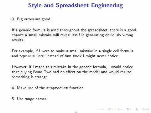
3. Big errors are good!
If a generic formula is used throughout the spreadsheet, there is a goodchance a small mistake will reveal itself in generating obviously wrongresults.
For example, if I were to make a small mistake in a single cell formulaand type Num Bnd1 instead of Num Bnd2 I might never notice.
However, if I made this mistake in the generic formula, I would noticethat buying Bond Two had no effect on the model and would realizesomething is strange.
4. Make use of the sumproduct function.
5. Use range names!
59
Style and Spreadsheet Engineering
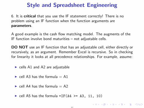
6. It is critical that you use the IF statement correctly! There is noproblem using an IF function when the function arguments areparameters.
A good example is the cash flow matching model. The augments of theIF function involve bond maturities – not adjustable cells.
DO NOT use an IF function that has an adjustable cell, either directly orrecursively, as an argument. Remember Excel is recursive. So in checkingfor linearity it looks at all precedence relationships. For example, assume:
I cells A1 and A2 are adjustable
I cell A3 has the formula = A1
I cell A4 has the formula = A2
I cell A5 has the formula =IF(A4 >= A3, 11, 10)
60
Style and Spreadsheet Engineering
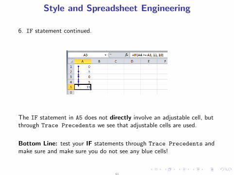
6. IF statement continued.
The IF statement in A5 does not directly involve an adjustable cell, butthrough Trace Precedents we see that adjustable cells are used.
Bottom Line: test your IF statements through Trace Precedents andmake sure and make sure you do not see any blue cells!
61
Style and Spreadsheet Engineering
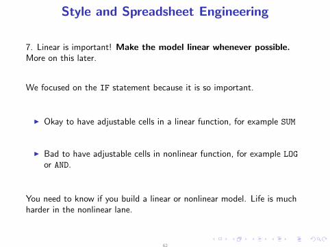
7. Linear is important! Make the model linear whenever possible.More on this later.
We focused on the IF statement because it is so important.
I Okay to have adjustable cells in a linear function, for example SUM
I Bad to have adjustable cells in nonlinear function, for example LOG
or AND.
You need to know if you build a linear or nonlinear model. Life is muchharder in the nonlinear lane.
62