3 recursive bayesian estimation
TRANSCRIPT

1
RecursiveBayesian Estimation
SOLO HERMELIN
Updated: 22.02.09 11.01.14
http://www.solohermelin.com

2
SOLOTable of Content Recursive Bayesian Estimation
Review of Probability
Conditional Probability
Total Probability Theorem
Conditional Probability - Bayes Formula
Statistical Independent Events
Expected Value or Mathematical Expectation
Variance and Central Moments
Characteristic Function and Moment-Generating Function
Probability Distribution and Probability Density Functions (Examples)
Normal (Gaussian) Distribution
Existence Theorems 1 & 2
Monte Carlo Method Estimation of the Mean and Variance of a Random Variable
Generating Discrete Random Variables
Existence Theorem 3Markov Processes
Functions of one Random Variable
The Laws of Large Numbers
Central Limit Theorem
Problem Definition
Stochastic Processes
3
SOLO
Table of Content (continue -1)Recursive Bayesian Estimation
Bayesian Estimation Introduction
Linear Gaussian Markov SystemsClosed-Form Solutions of Estimation
Kalman Filter
Extended Kalman FilterGeneral Bayesian Nonlinear Filters
Additive Gaussian Nonlinear FilterGauss – Hermite Quadrature ApproximationUnscented Kalman Filter
Monte Carlo Kalman Filter (MCKF)Non-Additive Non-Gaussian Nonlinear Filter
Nonlinear Estimation Using Particle FiltersImportance Sampling (IS)
Sequential Importance Sampling (SIS)
Sequential Importance Resampling (SIR)
Monte Carlo Particle Filter (MCPF)Bayesian Maximum Likelihood Estimate (Maximum Aposteriori – MAP Estimate)
4
SOLO
Table of Content (continue -2)Recursive Bayesian Estimation
References
Nonlinear Filters based on the Fokker-Planck Equation
5
SOLO Recursive Bayesian Estimation
kx1−kx
kz1−kz
0x 1x 2x
1z 2z kZ :11:1 −kZ
( )11, −− kk wxf
( )kk vxh ,
( )00 , wxf
( )11,vxh
( )11, wxf
( )22 ,vxh
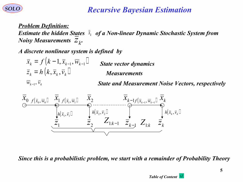
Since this is a probabilistic problem, we start with a remainder of Probability Theory
A discrete nonlinear system is defined by
( )( )kkk
kkk
vxkhz
wxkfx
,,
,,1 11
=−= −− State vector dynamics
Measurements
kk vw ,1− State and Measurement Noise Vectors, respectively
Problem Definition:Estimate the hidden States of a Non-linear Dynamic Stochastic System from Noisy Measurements .
kx
kz
Table of Content

6
SOLO
Pr (A) is the probability of the event A if
S nAAAA ∪∪∪= 21
1A 2A nA
jiOAA ji ≠∀/=∩
( ) 0Pr ≥A(1)
(3) If jiOAAandAAAA jin ≠∀/=∩∪∪∪= 21
( ) 1Pr =S(2)
then ( ) ( ) ( ) ( )nAAAA PrPrPrPr 21 +++=
Probability Axiomatic Definition
Probability Geometric Definition
Assume that the probability of an event in a geometric region A is defined as theratio between A surface to surface of S.
( ) ( )( )SSurface
ASurfaceA =Pr
( ) 0Pr ≥A(1)
( ) 1Pr =S(2)
(3) If jiOAAandAAAA jin ≠∀/=∩∪∪∪= 21
then ( ) ( ) ( ) ( )nAAAA PrPrPrPr 21 +++=
S
A
Review of ProbabilityA more detailed explanationof the subject is given in the“Probability” Presentation

7
SOLO
From those definition we can prove the following:( ) 0=/OP(1’)
Proof: OOSandOSS /=/∩/∪=( )
( ) ( ) ( ) ( ) 0PrPrPrPr3
=/⇒/+=⇒ OOSS
( ) ( )APAP −= 1(2’)
Proof: OAAandAAS /=∩∪= ( )( ) ( )
( ) ( ) ( ) ( )AAAAS Pr1PrPrPr1Pr32
−=⇒+==⇒
( ) 1Pr0 ≤≤ A(3’)
Proof: ( ) ( )( )
( )( ) 1Pr0Pr1Pr
1'2
≤⇒≥−= AAA( )
( )APr01
≤
( ) 0Pr ≥A(1) ( ) 1Pr =S(2) (3) If jiOAAandAAAA jin ≠∀/=∩∪∪∪= 21
then ( ) ( ) ( ) ( )nAAAA PrPrPrPr 21 +++=
( ) ( )AABAIf PrPr ≤⇒⊂(4’)
Proof: ( )( )
( ) ( ) ( ) ( )BAAABB PrPr0PrPrPr00
3
≤⇒≥+−=≥≥
( ) ( ) OAABandAABB /=∩−∪−=( ) ( ) ( ) ( )BABABA ∩−+=∪ PrPrPrPr(5’)
Proof: ( ) ( )( ) ( ) ( ) ( ) OABBAandABBAB
OABAandABABA
/=−∩∩−∪∩=/=−∩−∪=∪
( )( )
( ) ( )( )
( )( ) ( )
( ) ( ) ( ) ( )BABABAABBAB
ABABA∩−+=∪⇒
−+∩=
−+=∪PrPrPrPr
PrPrPr
PrPrPr3
3
Table of Content
Review of Probability

8
SOLO
Conditional Probability
S nAAAA ααα ∪∪∪= 21
1αA
jiOAA ji ≠∀/=∩
1αβA
mAAAB βββ ∪∪∪= 212αA
2αβA 1βA 2βA
Given two events A and B decomposed in elementary events
jiOAAandAAAAA ji
n
iin ≠∀/=∩=∪∪∪=
=αααααα
121
lkOAAandAAAAB lk
m
kkm ≠∀/=∩=∪∪∪=
=ββββββ
121
jiOAAandAAABA jir ≠∀/=∩∪∪∪=∩ αβαβαβαβαβ 21
( ) ( ) ( ) ( )nAAAA ααα PrPrPrPr 21 +++= ( ) ( ) ( ) ( )mAAAB βββ PrPrPrPr 21 +++=
( ) ( ) ( ) ( ) nmrAAABA r ,PrPrPrPr 21 ≤+++=∩ βαβαβα
We want to find the probability of A event under the condition that the event B had occurred designed as P (A|B)
( ) ( ) ( ) ( )( ) ( ) ( )
( )( )B
BA
AAA
AAABA
m
r
Pr
Pr
PrPrPr
PrPrPr|Pr
21
21 ∩=++++++
=βββ
βαβαβα
Review of Probability
9
SOLO
Conditional Probability S nAAAA ααα ∪∪∪= 21
1αA
jiOAA ji ≠∀/=∩
1αβA
mAAAB βββ ∪∪∪= 212αA
2αβA 1βA 2βA
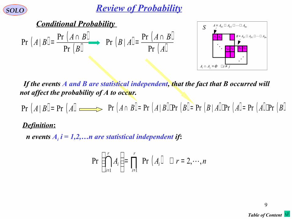
If the events A and B are statistical independent, that the fact that B occurred will not affect the probability of A to occur.
( ) ( )( )B
BABA
Pr
Pr|Pr
∩= ( ) ( )( )A
BAAB
Pr
Pr|Pr
∩=
( ) ( )ABA Pr|Pr = ( ) ( ) ( ) ( ) ( ) ( ) ( )BAAABBBABA PrPrPr|PrPr|PrPr ⋅=⋅=⋅=∩
Definition:
n events Ai i = 1,2,…n are statistical independent if:
( ) nrAAr
ii
r
ii ,,2PrPr
11
=∀=
∏==
Table of Content
Review of Probability
10
SOLO
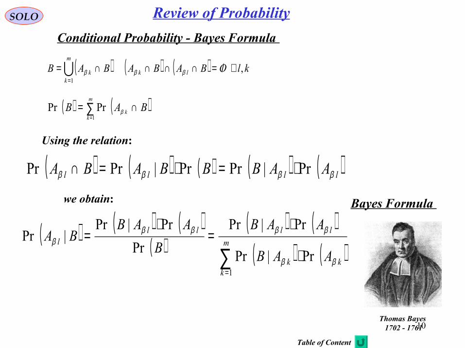
Conditional Probability - Bayes Formula
Using the relation:
( ) ( ) ( ) ( ) ( )llll AABBBABA ββββ Pr|PrPr|PrPr ⋅=⋅=∩
( ) ( ) ( ) klOBABABAB lk
m
kk ,
1
∀/=∩∩∩∩==
βββ
( ) ( )∑=
∩=m
kk BAB
1
PrPr β
we obtain:
( ) ( ) ( )( )
( ) ( )( ) ( )∑
=
⋅
⋅=
⋅=
m
kkk
lllll
AAB
AAB
B
AABBA
1
Pr|Pr
Pr|Pr
Pr
Pr|Pr|Pr
ββ
βββββ
Bayes Formula
Thomas Bayes 1702 - 1761
Table of Content
Review of Probability

11
SOLO
Total Probability Theorem
Table of Content
jiOAAandSAAA jin ≠∀/=∩=∪∪∪ 21If
we say that the set space S is decomposed in exhaustive andincompatible (exclusive) sets.
The Total Probability Theorem states that for any event B,its probability can be decomposed in terms of conditionalprobability as follows:
( ) ( ) ( ) ( )∑∑==
==n
ii
n
ii BPBABAB
11
|Pr,PrPr
Using the relation:
( ) ( ) ( ) ( ) ( )llll AABBBABA Pr|PrPr|PrPr ⋅=⋅=∩
( ) ( ) ( ) klOBABABAB lk
n
kk ,
1
∀/=∩∩∩∩==
( ) ( )∑=
∩=n
kk BAB
1
PrPr
For any event B
we obtain:
Review of Probability
12
SOLO
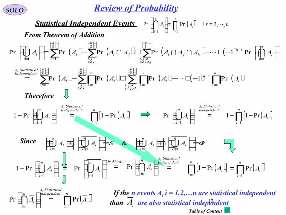
Statistical Independent Events
( ) ( ) ( ) ( )
( ) ( ) ( ) ( ) ( )∏∑∏∑∏∑
∑∑∑
=
−
≠≠=
≠=
=
=
−
≠≠
≠
==
−+−+−=
−+−+−=
n
ii
n
n
kjikji i
i
n
jiji i
i
n
ii
tIndependenlStatisticaA
n
ii
n
n
kjikji
kji
n
jiji
ji
n
ii
n
ii
AAAA
AAAAAAAA
i
1
13
,.
3
1
2
.
2
1
1
1
1
13
,.
2
.
1
11
Pr1PrPrPr
Pr1PrPrPrPr
From Theorem of Addition
Therefore
( )[ ]∏==
−=
−n
ii
tIndependenlStatisticaA
n
ii AA
i
11
Pr1Pr1 ( )[ ]∏==
−−=
n
ii
tIndependenlStatisticaA
n
ii AA
i
11
Pr11Pr
Since OAASAAn
ii
n
ii
n
ii
n
ii /=
=
====
1111
&
=
−==
n
ii
n
ii AA
11
PrPr1
( )∏==
=
n
ii
tIndependenlStatisticaA
n
ii AA
i
11
PrPr If the n events Ai i = 1,2,…n are statistical independent than are also statistical independent iA
( )∏=
=n
iiA
1
Pr
==
n
ii
MorganDe
A1
Pr ( )[ ]∏=
−=n
ii
tIndependenlStatisticaA
A
i
1
Pr1
( ) nrAAr
ii
r
ii ,,2PrPr
11
=∀=
∏==
Table of Content
Review of Probability

13
SOLO Review of Probability
Expected Value or Mathematical Expectation
Given a Probability Density Function p (x) we define the Expected Value
For a Continuous Random Variable: ( ) ( )∫+∞
∞−
= dxxpxxE X:
For a Discrete Random Variable: ( ) ( )∑=k
kXk xpxxE :
For a general function g (x) of the Random Variable x: ( )[ ] ( ) ( )∫
+∞
∞−
= dxxpxgxgE X:
( )xp
x
0 ∞+∞−
0.1
( )xE
( )( )
( )∫
∫∞+
∞−
+∞
∞−=dxxp
dxxpxxE
X
X
:
The Expected Value is the center of surface enclosed between the Probability Density Function and x axis.
Table of Content

14
SOLO Review of Probability
Variance
Given a Probability Density Functions p (x) we define the Variance
( ) ( )[ ] ( ) ( )[ ] ( ) ( ) 22222 2: xExExExExxExExExVar −=+−=−=
Central Moment
( ) kk xEx =:'µ
Given a Probability Density Functions p (x) we define the Central Moment of order k about the origin
( ) ( )[ ] ( ) ( )∑=
−−−
=−=
k
j
jkj
jkkk xE
j
kxExEx
0
'1: µµ
Given a Probability Density Functions p (x) we define the Central Moment of order k about the Mean E (x)
Table of Content

15
SOLO Review of Probability
Moments
Normal Distribution ( ) ( ) ( )[ ]σπ
σσ2
2/exp;
22xxpX
−=
[ ] ( ) −⋅
=oddnfor
evennfornxE
nn
0
131 σ
[ ]( )
+=
=−⋅=
+ 12!22
2131
12 knfork
knforn
xEkk
n
n
σπ
σ
Proof:
Start from: and differentiate k time with respect to a( ) 0exp 2 >=−∫∞
∞−
aa
dxxaπ
Substitute a = 1/(2σ2) to obtain E [xn]
( ) ( )0
2
1231exp
1222 >−⋅=− +
∞
∞−∫ a
a
kdxxax
kkk π
[ ] ( ) ( )[ ] ( ) ( )[ ]( ) ( ) 12
!
0
122/
0
222221212
!22
exp2
22
2/exp2
22/exp
2
1
2
+∞+=
∞∞
∞−
++
=−=
−=−=
∫
∫∫
kk
k
k
kxy
kkk
kdyyy
xdxxxdxxxxE
σπσ
σπ
σσπ
σσπ
σ
Now let compute:
[ ] [ ]( )2244 33 xExE == σ
Chi-square

16
SOLO Review of Probability
Functions of one Random Variable
Let y = g (x) a given function of the random variable x defined o the domain Ω, withprobability distribution pX (x). We want to find pY (y).
Fundamental Theorem
Assume x1, x2, …, xn all the solutions of the equation( ) ( ) ( )nxgxgxgy ==== 21
( ) ( )( )
( )( )
( )( )n
nXXXY xg
xp
xg
xp
xg
xpyp
''' 2
2
1
1 +++=
( ) ( )xd
xgdxg =:'
Proof
( ) ( ) ( ) ( ) ( )( )∑∑∑
===
==±≤≤=+≤≤=n
i i
iXn
iiiX
n
iiiiY yd
xg
xpxdxpxdxxxydyYyydyp
111 'PrPr:
q.e.d.

17
SOLO Review of Probability
Functions of one Random Variable (continue – 1)
Example 1
bxay += ( )
−=
a
byp
ayp XY
1
Example 2
x
ay = ( )
=
y
ap
y
ayp XY 2
Example 32xay = ( ) ( )yU
a
yp
a
yp
yayp XXY
−+
=
2
1
Example 4
xy = ( ) ( ) ( )[ ] ( )yUypypyp XXY −+=
Table of Content

18
SOLO Review of Probability
Characteristic Function and Moment-Generating Function
Given a Probability Density Functions pX (x) we define the Characteristic Function or Moment Generating Function
( ) ( )[ ]( ) ( ) ( ) ( )
( ) ( )
===Φ
∑
∫∫+∞
∞−
+∞
∞−
xX
XX
X
discretexxpxj
continuousxxPdxjdxxpxjxjE
ω
ωωωω
exp
expexpexp:
This is in fact the complex conjugate of the Fourier Transfer of the Probability Density Function. This function is always defined since the sufficient condition of the existence of a Fourier Transfer :
Given the Characteristic Function we can find the Probability Density Functions pX (x) using the Inverse Fourier Transfer:
( )( )
( ) ∞<== ∫∫+∞
∞−
≥+∞
∞−
10
dxxpdxxp X
xp
X
( ) ( ) ( )∫+∞
∞−
Φ−= ωωωπ
dxjxp XX exp2
1
is always fulfilled.

19
SOLO Review of Probability
Properties of Moment-Generating Function
( ) ( ) ( )∫+∞
∞−
=Φdxxpxxjj
d
dX
X ωω
ωexp
( ) ( ) 10
==Φ ∫+∞
∞−=
dxxpXX ωω
( ) ( ) ( )xEjdxxpxjd
dX
X ==Φ∫
+∞
∞−=0ωωω
( ) ( ) ( ) ( )∫+∞
∞−
=Φdxxpxxjj
d
dX
X 22
2
2
exp ωω
ω ( ) ( ) ( ) ( ) ( )2222
0
2
2
xEjdxxpxjd
dX
X ==Φ∫
+∞
∞−=ωωω
( ) ( ) ( ) ( )∫+∞
∞−
=Φdxxpxxjj
d
dX
nn
n
X
n
ωω
ωexp
( ) ( ) ( ) ( ) ( )nnX
nn
nX
n
xEjdxxpxjd
d ==Φ∫
+∞
∞−=0ωωω
( ) ( ) ( )∫+∞
∞−
=Φ dxxpxj XX ωω exp
This is the reason why ΦX (ω) is also called the Moment-Generation Function.

20
SOLO Review of Probability
Properties of Moment-Generating Function
( ) ( ) ( ) ( ) ( )
( ) ( ) ( ) ( ) ( ) ( )
+++++=
+Φ++Φ+Φ+Φ=Φ===
=
nn
nn
Xn
XXXX
xEn
jxE
jxE
j
d
d
nd
d
d
d
!!2!11
!
1
!2
1
22
0
2
0
2
2
00
ωωω
ωω
ωωω
ωωω
ωωωωωω
ω
Develop ΦX (ω) in a Taylor series
( ) ( ) ( )∫+∞
∞−
=Φ dxxpxj XX ωω exp

21
SOLO Review of Probability
Probability Distribution and Probability Density Functions (Examples)
(2) Poisson’s Distribution ( ) ( )00 exp!
, kk
knkp
k
−≈
(1) Binomial (Bernoulli) ( ) ( ) ( ) ( ) knkknk ppk
npp
knk
nnkp −− −
=−
−= 11
!!
!,
0 1 2 3 4 5 6 7 8 9 10 11 12 13 14 k
( )nkP ,
(3) Normal (Gaussian) ( ) ( ) ( )[ ]σπ
σµσµ2
2/exp,;
22−−= xxp
(4) Laplacian Distribution ( )
−−=
b
x
bbxp
µµ exp
2
1,;

22
SOLO Review of Probability
Probability Distribution and Probability Density Functions (Examples)
(5) Gama Distribution ( )( )( )
<
≥Γ
−=
−
00
0/exp
,;1
x
xxk
x
kxpk
kθθ
θ
(6) Beta Distribution( ) ( )
( )( )
( ) ( ) ( ) 11
1
0
11
11
11
1,; −−
−−
−−
−ΓΓ+Γ=
−
−=∫
βα
βα
βα
βαβαβα xx
duuu
xxxp
(7) Cauchy Distribution ( ) ( )
+−
=22
0
0
1,;
γγ
πγ
xxxxp

23
SOLO Review of Probability
Probability Distribution and Probability Density Functions (Examples)
SOLO
(8) Exponential Distribution
( ) ( )
<≥−
=00
0exp;
x
xxxp
λλλ
(9) Chi-square Distribution
( )( )
( ) ( )
<
≥−Γ=
−
00
02/exp2/
2/1;
12/
2/
x
xxxkkxp
k
k
Γ is the gamma function ( ) ( )∫∞
− −=Γ0
1 exp dttta a
(10) Student’s t-Distribution
( ) ( )[ ]( ) ( ) ( ) 2/12 /12/
2/1; ++Γ
+Γ= νννπννν
xxp

24
SOLO Review of Probability
Probability Distribution and Probability Density Functions (Examples)
SOLO
(11) Uniform Distribution (Continuous)
( )
>>
≤≤−=
bxxa
bxaabbaxp
0
1,;
(12) Rayleigh Distribution
( )2
2
2
2exp
;σ
σσ
−
=
xx
xp
(13) Rice Distribution
( )
+−=
202
2
22
2exp
,;σσ
σσ vx
I
vxx
vxp

25
SOLO Review of Probability
Probability Distribution and Probability Density Functions (Examples)
(14) Weibull Distribution
SOLO
( )
<
>≥
−−
−
=
−
00
0,,exp,,;
1
x
xxx
xpαγµ
αµ
αµ
αγ
αµγ
γγ
Table of Content
26
SOLO Review of Probability
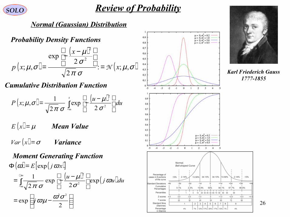
Normal (Gaussian) Distribution
Karl Friederich Gauss1777-1855
( )
( )
( )σµσπσµ
σµ ,;:2
2exp
,;2
2
x
x
xp N=
−−=
( ) ( )∫∞−
−−=x
duu
xP2
2
2exp
2
1,;
σµ
σπσµ
( ) µ=xE
( ) σ=xVar
( ) ( )[ ]( ) ( )
−=
−−=
=Φ
∫∞+
∞−
2exp
exp2
exp2
1
exp
22
2
2
σωµω
ωσµ
σπ
ωω
j
duuju
xjE
Probability Density Functions
Cumulative Distribution Function
Mean Value
Variance
Moment Generating Function

27
SOLO Review of Probability
Moments
Normal Distribution ( ) ( ) ( )[ ] ( )σσπ
σσ ,0;:2
2/exp,0;
22
xx
xpX N=−=
[ ] ( ) −⋅
=oddnfor
evennfornxE
nn
0
131 σ
[ ]( )
+=
=−⋅=
+ 12!22
2131
12 knfork
knforn
xEkk
n
n
σπ
σ
Proof:
Start from: and differentiate k time with respect to a( ) 0exp 2 >=−∫∞
∞−
aa
dxxaπ
Substitute a = 1/(2σ2) to obtain E [xn]
( ) ( )0
2
1231exp
1222 >−⋅=− +
∞
∞−∫ a
a
kdxxax
kkk π
[ ] ( ) ( )[ ] ( ) ( )[ ]( ) ( ) 12
!
0
122/
0
222221212
!22
exp2
22
2/exp2
22/exp
2
1
2
+∞+=
∞∞
∞−
++
=−=
−=−=
∫
∫∫
kk
k
k
kxy
kkk
kdyyy
xdxxxdxxxxE
σπσ
σπ
σσπ
σσπ
σ
Now let compute:
[ ] [ ]( )2244 33 xExE == σ
Chi-square
28
SOLO Review of Probability
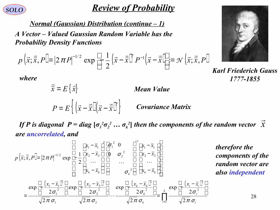
Normal (Gaussian) Distribution (continue – 1)
Karl Friederich Gauss1777-1855
( ) ( ) ( ) ( )PxxxxPxxPPxxpT
,;:2
1exp2,; 12/1
N=
−−−= −−π
A Vector – Valued Gaussian Random Variable has theProbability Density Functions
where
xEx
= Mean Value
( ) ( ) TxxxxEP −−= Covariance Matrix
If P is diagonal P = diag [σ12σ2
2 … σk2] then the components of the random vector
are uncorrelated, andx
( )
( ) ( ) ( ) ( )
∏=
−
−
−−=
−−
−−
−−=
−
−−
−
−−
−=
k
i i
i
ii
k
k
kk
kkk
T
kk
xxxxxxxx
xx
xx
xx
xx
xx
xx
PPxxp
1
2
2
2
2
2
22
222
1
21
211
22
11
1
2
22
21
22
11
2/1
2
2exp
2
2exp
2
2exp
2
2exp
0
0
2
1exp2,;
σπσ
σπσ
σπσ
σπσ
σ
σ
σ
π
therefore the components of the random vector are also independent

29
SOLO Review of Probability
The Laws of Large Numbers
The Law of Large Numbers is a fundamental concept in statistics and probability thatdescribes how the average of randomly selected sample of a large population is likelyto be close to the average of the whole population. There are two laws of large numbersthe Weak Law and the Strong Law.
The Weak Law of Large Numbers
The Weak Law of Large Numbers states that if X1,X2,…,Xn,… is an infinite sequenceof random variables that have the same expected value μ and variance σ2, and areuncorrelated (i.e., the correlation between any two of them is zero), then
( ) nXXX nn /: 1 ++=
converges in probability (a weak convergence sense) to μ . We have
∞→=<− nforX n 1Pr εµconverges in probability
The Strong Law of Large Numbers The Strong Law of Large Numbers states that if X1,X2,…,Xn,… is an infinite sequenceof random variables that have the same expected value μ and variance σ2, and areuncorrelated (i.e., the correlation between any two of them is zero), and E (|Xi|) < ∞then ,i.e. converges almost surely to μ. ∞→== nforX n 1Pr µ
converges almost surely

3030
SOLO Review of Probability
The Law of Large Numbers
Differences between the Weak Law and the Strong Law
The Weak Law states that, for a specified large n, (X1 + ... + Xn) / n is likely to be near μ. Thus, it leaves open the possibility that | (X1 + ... + Xn) / n − μ | > ε happens an infinite number of times, although it happens at infrequent intervals.
The Strong Law shows that this almost surely will not occur. In particular, it implies that with probability 1, we have for any positive value ε, the inequality | (X1 + ... + Xn) / n − μ | > ε is true only a finite number of times (as opposed to an infinite, but infrequent, number of times).
Almost sure convergence is also called strong convergence of random variables. This version is called the strong law because random variables which converge strongly (almost surely) are guaranteed to converge weakly (in probability). The strong law implies the weak law.
3131
SOLO Review of Probability
The Law of Large Numbers
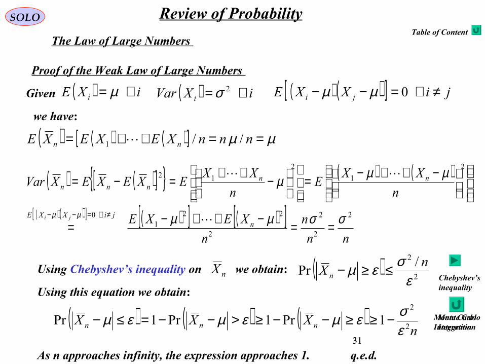
Proof of the Weak Law of Large Numbers
( ) iXE i ∀= µ ( ) iXVar i ∀= 2σ ( ) ( )[ ] jiXXE ji ≠∀=−− 0µµ
( ) ( ) ( )[ ] µµ ==++= nnnXEXEXE nn //1
( ) ( )[ ] ( ) ( )
( ) ( )[ ] ( )[ ] ( )[ ]nn
n
n
XEXE
n
XXE
n
XXEXEXEXVar
njiXXE
nnnnn
ji 2
2
2
2
221
0
2
1
2
12
σσµµ
µµµ
µµ
==−++−=
−++−=
−++=−=
≠∀=−−
Given
we have:
Using Chebyshev’s inequality on we obtain:nX ( )2
2 /Pr
εσεµ n
X n ≤≥−Using this equation we obtain:
( ) ( ) ( )n
XXX nnn 2
2
1Pr1Pr1Prεσεµεµεµ −≥≥−−≥>−−=≤−
As n approaches infinity, the expression approaches 1.
Chebyshev’sinequality
q.e.d.
Monte CarloIntegration
Monte CarloIntegration
Table of Content
3232
SOLO Review of Probability
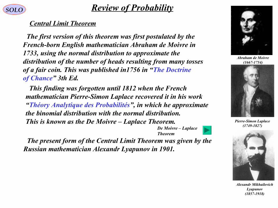
Central Limit Theorem
The first version of this theorem was first postulated by the French-born English mathematician Abraham de Moivre in1733, using the normal distribution to approximate thedistribution of the number of heads resulting from many tossesof a fair coin. This was published in1756 in “The Doctrine of Chance” 3th Ed.
Pierre-Simon Laplace(1749-1827)
Abraham de Moivre(1667-1754)
This finding was forgotten until 1812 when the French mathematician Pierre-Simon Laplace recovered it in his work “Théory Analytique des Probabilités”, in which he approximate the binomial distribution with the normal distribution. This is known as the De Moivre – Laplace Theorem.
De Moivre – Laplace Theorem
The present form of the Central Limit Theorem was given by theRussian mathematician Alexandr Lyapunov in 1901.
Alexandr MikhailovichLyapunov
(1857-1918)

3333
SOLO Review of Probability
Central Limit Theorem (continue – 1)
Let X1, X2, …, Xm be a sequence of independent random variables with the sameprobability distribution function pX (x). Define the statistical mean:
m
XXXX m
m
+++=
21
( ) ( ) ( ) ( ) µ=+++
=m
XEXEXEXE m
m
21
( ) ( )[ ] ( ) ( ) ( )mm
m
m
XXXEXEXEXVar m
mmmX m
2
2
22
2122 σσµµµσ ==
−++−+−
=−==
Define also the new random variable
( ) ( ) ( ) ( )m
XXXXEXY m
X
mm
mσ
µµµσ
−++−+−=−= 21:
We have:
The probability distribution of Y tends to become gaussian (normal) as m tends to infinity, regardless of the probability distribution of the random variable, as long as the mean μ and the variance σ2 are finite.

3434
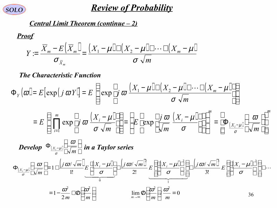
SOLO Review of Probability
Central Limit Theorem (continue – 2)
( ) ( ) ( ) ( )m
XXXXEXY m
X
mm
mσ
µµµσ
−++−+−=−= 21:
Proof
The Characteristic Function
( ) ( )[ ] ( ) ( ) ( )
( ) ( )( )
m
X
m
im
i
i
mY
m
X
m
jE
m
XjE
m
XXXjEYjE
i
Φ=
−=
−=
−++−+−==Φ
−=
∏ ωσ
µωσ
µω
σµµµωωω
σµexpexp
expexp
1
21
( )( ) ( ) ( ) ( ) ( ) ( )
0/lim2
1
!3
/
!2
/
!1
/1
2222
33
1
22
0
=
Ο/
Ο/+−=
+
−+
−+
−+=
Φ
∞→
−
mmmm
XE
mjXE
mjXE
mj
m
m
iiiX i
ωωωω
σµω
σµω
σµωω
σµ
Develop in a Taylor series( )
Φ −
miX
ω
σµ
35
SOLO Review of Probability
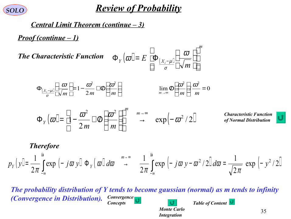
Central Limit Theorem (continue – 3)
Proof (continue – 1)
The Characteristic Function ( ) ( )
m
XYm
Ei
Φ=Φ −
ωωσ
µ
( ) 0/lim2
12222
=
Ο/
Ο/+−=
Φ
∞→− mmmmm mX i
ωωωωωσ
µ
( ) ( )2/exp2
1 222
ωωωω −→
Ο/+−=Φ
∞→mm
Y mm
Therefore
( ) ( ) ( ) ( ) ( )2/exp2
12/exp
2
1exp
2
1 22 ydyjdyjypm
YY −=−−→Φ−= ∫∫+ ∞
∞−
∞→+ ∞
∞− πωωω
πωωω
π
The probability distribution of Y tends to become gaussian (normal) as m tends to infinity(Convergence in Distribution).
Characteristic Functionof Normal Distribution
ConvergenceConcepts
Monte CarloIntegration
Table of Content
36
SOLO Review of Probability
Central Limit Theorem (continue – 2)
( ) ( ) ( ) ( )m
XXXXEXY m
X
mm
mσ
µµµσ
−++−+−=−= 21:
Proof
The Characteristic Function
( ) ( )[ ] ( ) ( ) ( )
( ) ( )( )
m
X
m
im
i
i
mY
m
X
m
jE
m
XjE
m
XXXjEYjE
i
Φ=
−=
−=
−++−+−==Φ
−=
∏ ωσ
µωσ
µω
σµµµωωω
σµexpexp
expexp
1
21
( )( ) ( ) ( ) ( ) ( ) ( )
0/lim2
1
!3
/
!2
/
!1
/1
2222
33
1
22
0
=
Ο/
Ο/+−=
+
−+
−+
−+=
Φ
∞→
−
mmmm
XE
mjXE
mjXE
mj
m
m
iiiX i
ωωωω
σµω
σµω
σµωω
σµ
Develop in a Taylor series( )
Φ −
miX
ω
σµ

37
SOLO Review of Probability
Central Limit Theorem (continue – 3)
Proof (continue – 1)
The Characteristic Function ( ) ( )
m
XYm
Ei
Φ=Φ −
ωωσ
µ
( ) 0/lim2
12222
=
Ο/
Ο/+−=
Φ
∞→− mmmmm mX i
ωωωωωσ
µ
( ) ( )2/exp2
1 222
ωωωω −→
Ο/+−=Φ
∞→mm
Y mm
Therefore
( ) ( ) ( ) ( ) ( )2/exp2
12/exp
2
1exp
2
1 22 ydyjdyjypm
YY −=−−→Φ−= ∫∫+ ∞
∞−
∞→+ ∞
∞− πωωω
πωωω
π
The probability distribution of Y tends to become gaussian (normal) as m tends to infinity(Convergence in Distribution).
Characteristic Functionof Normal Distribution
ConvergenceConcepts
Table of Content
38
SOLO Review of Probability
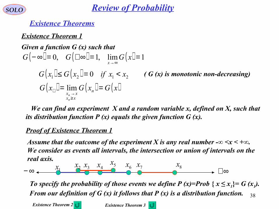
Existence Theorems
Existence Theorem 1
Given a function G (x) such that
( ) ( ) ( ) 1lim,1,0 ==∞+=∞−∞→
xGGGx
( ) ( ) 2121 0 xxifxGxG <=≤ ( G (x) is monotonic non-decreasing)
( ) ( ) ( )xGxGxG n
xxxx
n
n
==≥→+ lim
We can find an experiment X and a random variable x, defined on X, such thatits distribution function P (x) equals the given function G (x).
Proof of Existence Theorem 1
Assume that the outcome of the experiment X is any real number -∞ <x < +∞. We consider as events all intervals, the intersection or union of intervals on thereal axis.
5x1x 2x 3x 4x 6x 7x 8x
∞− ∞+To specify the probability of those events we define P (x)=Prob x ≤ x1= G (x1).From our definition of G (x) it follows that P (x) is a distribution function.
Existence Theorem 2 Existence Theorem 3

39
SOLO Review of Probability
Existence Theorems
Existence Theorem 2
If a function F (x,y) is such that
( ) ( ) ( )( ) ( ) ( ) ( ) 0,,,,
1,,0,,
11122122 ≥+−−=+∞∞+=−∞=∞−yxFyxFyxFyxF
FxFyF
for every x1 < x2, y1 < y2, then two random variables x and y can be found such thatF (x,y) is their joint distribution function.
Proof of Existence Theorem 2
Assume that the outcome of the experiment X is any real number -∞ <x < +∞.Assume that the outcome of the experiment Y is any real number -∞ <y < +∞. We consider as events all intervals, the intersection or union of intervals on thereal axes x and y.
To specify the probability of those events we define P (x,y)=Prob x ≤ x1, y ≤ y1, = F (x1,y1).From our definition of F (x,y) it follows that P (x,y) is a joint distribution function.
The proof is similar to that in the Existence Theorem 1

40
SOLO Review of ProbabilityMonte Carlo Method
Monte Carlo methods are a class of computational algorithms that rely on repeated random sampling to compute their results. Monte Carlo methods are often used when simulating physical and mathematical systems. Because of their reliance on repeated computation and random or pseudo-random numbers, Monte Carlo methods are most suited to calculation by a computer. Monte Carlo methods tend to be used when it is infeasible or impossible to compute an exact result with a deterministic algorithm.
The term Monte Carlo method was coined in the 1940s by physicists Stanislaw Ulam, Enrico Fermi, John von Neumann, and Nicholas Metropolis, working on nuclear weapon projects in the Los Alamos National Laboratory (reference to the Monte Carlo Casino in Monaco where Ulam's uncle would borrow money to gamble)
Stanislaw Ulam1909 - 1984
Enrico - Fermi1901 - 1954
John von Neumann1903 - 1957
Monte Carlo Casino
Nicholas Constantine Metropolis
(1915 –1999)

41
SOLO Review of Probability
Monte Carlo Approximation
Monte Carlo runs, generate a set of random samples that approximate the distribution p (x). So, with P samples, expectations with respect to the filtering distribution are approximated by
( ) ( ) ( )( )∑∫=
≈P
L
LxfP
dxxpxf1
1
and , in the usual way for Monte Carlo, can give all the moments etc. of the distribution up to some degree of approximation.
( ) ( )∑∫=
≈==P
L
LxP
dxxpxxE1
1
1µ
( ) ( ) ( ) ( )( )∑∫=
−≈−=−=P
L
nLnnn x
PdxxpxxE
1111
1 µµµµ
Table of Content
x(L) are generated (draw) samples from distribution p (x)( ) ( )xpx L ~

42
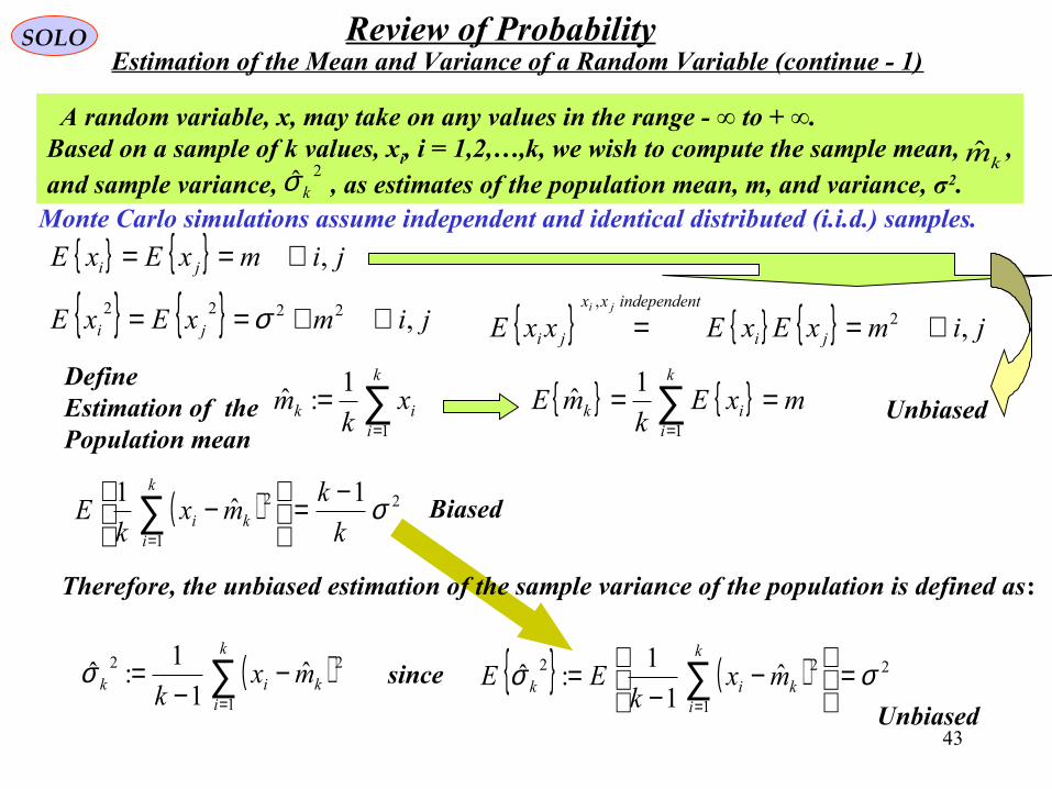
SOLO Review of ProbabilityEstimation of the Mean and Variance of a Random Variable (Unknown Statistics)
jimxExE ji ,∀==
DefineEstimation of thePopulation mean
∑=
=k
iik x
km
1
1:ˆ
A random variable, x, may take on any values in the range - ∞ to + ∞.Based on a sample of k values, xi, i = 1,2,…,k, we wish to compute the sample mean, ,and sample variance, , as estimates of the population mean, m, and variance, σ2.
2ˆkσkm
( )
( ) ( ) ( )[ ] ( ) ( )[ ]2
1
2
1
2222
22222
1 112
1
2
2
11
2
1
2
111
1
11
121
112
1
ˆˆ21
ˆ1
σσ
σσσ
k
k
kk
mkmkkk
mmkk
mk
xxk
Exk
xExEk
mxmxEk
mxk
E
k
i
k
i
k
i
k
ll
k
jj
k
jjii
k
k
iik
k
ii
k
iki
−=
−=
++−+++−−+=
+
−=
+−=
−
∑
∑
∑ ∑∑∑
∑∑∑
=
=
= ===
===
jimxExE ji ,2222 ∀+== σ
mxEk
mEk
iik == ∑
=1
1ˆ
jimxExExxE ji
tindependenxx
ji
ji
,2,
∀==
Compute
Biased
Unbiased
Monte Carlo simulations assume independent and identical distributed (i.i.d.) samples.
43
SOLO Review of ProbabilityEstimation of the Mean and Variance of a Random Variable (continue - 1)
jimxExE ji ,∀==
DefineEstimation of thePopulation mean
∑=
=k
iik x
km
1
1:ˆ
A random variable, x, may take on any values in the range - ∞ to + ∞.Based on a sample of k values, xi, i = 1,2,…,k, we wish to compute the sample mean, ,and sample variance, , as estimates of the population mean, m, and variance, σ2.
2ˆkσkm
( ) 2
1
2 1ˆ
1 σk
kmx
kE
k
iki
−=
−∑
=
jimxExE ji ,2222 ∀+== σ
mxEk
mEk
iik == ∑
=1
1ˆ
jimxExExxE ji
tindependenxx
ji
ji
,2,
∀==
Biased
Unbiased
Therefore, the unbiased estimation of the sample variance of the population is defined as:
( )∑=
−−
=k
ikik mx
k 1
22 ˆ1
1:σ since ( ) 2
1
22 ˆ1
1:ˆ σσ =
−
−= ∑
=
k
ikik mx
kEE
Unbiased
Monte Carlo simulations assume independent and identical distributed (i.i.d.) samples.

44
SOLO Review of ProbabilityEstimation of the Mean and Variance of a Random Variable (continue - 2)
A random variable, x, may take on any values in the range - ∞ to + ∞.Based on a sample of k values, xi, i = 1,2,…,k, we wish to compute the sample mean, ,and sample variance, , as estimates of the population mean, m, and variance, σ2.
2ˆkσkm
mxEk
mEk
iik == ∑
=1
1ˆ
( ) 2
1
22 ˆ1
1:ˆ σσ =
−
−= ∑
=
k
ikik mx
kEE
Monte Carlo simulations assume independent and identical distributed (i.i.d.) samples.

45
SOLO Review of ProbabilityEstimation of the Mean and Variance of a Random Variable (continue - 3)
mxEk
mEk
iik == ∑
=1
1ˆ ( ) 2
1
22 ˆ1
1:ˆ σσ =
−
−= ∑
=
k
ikik mx
kEE
We found:
Let Compute:
( ) ( )
( ) ( ) ( )
( ) ( ) ( ) k
mxEmxEmxEk
mxmxEmxEk
mxk
Emxk
EmmE
k
i
k
ijj
ji
k
ii
k
i
k
ijj
ji
k
ii
k
ii
k
iikmk
2
1 100
1
2
2
1 11
2
2
2
1
2
1
22ˆ
2
1
1
11ˆ:
σ
σ
σ
=
−−+−=
−−+−=
−=
−=−=
∑ ∑∑
∑∑∑
∑∑
=≠==
=≠==
==
( ) k
mmE kmk
222
ˆ ˆ:σσ =−=

46
SOLO Review of ProbabilityEstimation of the Mean and Variance of a Random Variable (continue - 4)
Let Compute:
( ) ( ) ( )
( ) ( ) ( ) ( )[ ]
( ) ( ) ( ) ( )
−−
−+−
−−+−
−=
−−+−−+−
−=
−−+−
−=
−−
−=−=
∑∑
∑
∑∑
==
=
==
2
22
11
2
2
2
1
22
2
2
1
22
2
1
22222
ˆ
ˆ11
ˆ2
1
1
ˆˆ21
1
ˆ1
1ˆ
1
1ˆ:2
σ
σ
σσσσσσ
k
k
ii
kk
ii
k
ikkii
k
iki
k
ikik
mmk
kmx
k
mmmx
kE
mmmmmxmxk
E
mmmxk
Emxk
EEk
( ) ( ) ( ) ( ) ( ) ( ) ( ) ( ) ( )
( ) ( ) ( ) ( )
( ) ( ) ( ) ( )
( ) ( ) ( ) ( )
( ) ( ) ( ) ( )
k
k
k
ii
kk
ii
k
k
k
ii
k
k
ii
k
kk
ii
k
k
k
k
ii
k
kk
i
k
ijj
ji
k
k
ii
mmEk
kmxE
k
mmEmxE
k
mmEk
mxEk
mxEk
mmEkmxE
k
mmE
mmEk
kmxE
k
mmEmxEmxEmxE
kk
/
22
10
2
0
10
2
3
1
22
1
2
2
/
2
1
3
2
0
44
2
2
1
2
2
/
2
1 1
22
1
4
2
2
ˆ
2
222
22
22
4
2
ˆ1
2
1
ˆ4
1
ˆ4
1
2
1
ˆ2
1
ˆ4
ˆ11
ˆ4
1
1
σ
σσσ
σσ
σσµ
σ
σσ
σ
σσ
−−
−−−
−−−−
−+
−−
−−−
−+−−
−+
+−−
+−−−+
−−+−−
≈
∑∑
∑∑∑
∑∑ ∑∑
==
===
==≠==
Since (xi – m), (xj - m) and are all independent for i ≠ j:( )kmm ˆ−

47
SOLO Review of ProbabilityEstimation of the Mean and Variance of a Random Variable (continue - 4)
Since (xi – m), (xj - m) and are all independent for i ≠ j:( )kmm ˆ−
( )( )( ) ( ) ( ) ( )
( ) ( ) ( ) ( ) ( ) ( ) ( ) 4
2
24
224
44
2
4
44
2
2
2
4
2
4
242
ˆ
ˆ11
7
11
2
1
2
1
2
ˆ11
4
1
1
12
k
k
mmEk
k
k
k
k
k
kk
k
k
k
mmEk
k
kk
kk
k
kk
−−
+−+−+
−=
−−
−−
−+
+−−
+−
+−−+
−≈
σµσσσ
σσσµσσ
kk
442
ˆ 2
σµσσ
−≈ ( ) 44 : mxE i −=µ
( ) ( ) ( ) ( ) ( ) ( ) ( ) ( ) ( )
( ) ( ) ( ) ( )
( ) ( ) ( ) ( )
( ) ( ) ( ) ( )
( ) ( ) ( ) ( )
k
k
k
ii
kk
ii
k
k
k
ii
k
k
ii
k
kk
ii
k
k
k
k
ii
k
kk
i
k
ijj
ji
k
k
ii
mmEk
kmxE
k
mmEmxE
k
mmEk
mxEk
mxEk
mmEkmxE
k
mmE
mmEk
kmxE
k
mmEmxEmxEmxE
kk
/
22
10
2
0
10
2
3
1
22
1
2
2
/
2
1
3
2
0
44
2
2
1
2
2
/
2
1 1
22
1
4
2
2
ˆ
2
222
22
22
4
2
ˆ1
2
1
ˆ4
1
ˆ4
1
2
1
ˆ2
1
ˆ4
ˆ11
ˆ4
1
1
σ
σσσ
σσ
σσµ
σ
σσ
σ
σσ
−−
−−−
−−−−
−+
−−
−−−
−+−−
−+
+−−
+−−−+
−−+−−
≈
∑∑
∑∑∑
∑∑ ∑∑
==
===
==≠==

48
SOLO Review of ProbabilityEstimation of the Mean and Variance of a Random Variable (continue - 5)
mxEk
mEk
iik == ∑
=1
1ˆ
( ) 2
1
22 ˆ1
1:ˆ σσ =
−
−= ∑
=
k
ikik mx
kEE
We found:
( ) k
mmE kmk
222
ˆ ˆ:σσ =−=
( ) ( )k
mxk
EEk
ikik
k
44
2
2
1
22222
ˆˆ
1
1ˆ:2
σµσσσσσ
−≈
−−
−=−= ∑
=
( ) 44 : mxE i −=µ
Kurtosis of random variable xiDefine
44:
σµλ =
( ) ( ) ( )k
mxk
EEk
ikik
k
42
2
1
22222
ˆ
1ˆ
1
1ˆ:2
σλσσσσσ
−≈
−−
−=−= ∑
=

49
SOLO Review of ProbabilityEstimation of the Mean and Variance of a Random Variable (continue - 6)
[ ] ϕσσσ σσ =≤≤ 2ˆ
2k
2
kˆ-0Prob n
For high values of k, according to the Central Limit Theorem the estimations of mean and of variance are approximately Gaussian Random Variables.
km2ˆkσ
We want to find a region around that will contain σ2 with a predefined probabilityφ as function of the number of iterations k.
2ˆkσ
Since are approximately Gaussian Random Variables nσ is given by solving:
2ˆkσ
ϕζζπ
σ
σ
=
−∫
+
−
n
n
d2
2
1exp
2
1
nσ φ
1.000 0.6827
1.645 0.9000
1.960 0.9500
2.576 0.9900
Cumulative Probability within nσ
Standard Deviation of the Mean for aGaussian Random Variable
22k
22 1ˆ-
1 σλσσσλσσ k
nk
n−≤≤−−
22k
2 11
ˆ-11 σλσσλ
σσ
−−≤≤
+−−
kn
kn
( ) ( ) ( ) ( )( )42222 1,0;ˆ~ˆ&,0;ˆ~ˆ σλσσσσ −−− kkkk kmmmk NN
50
SOLO Review of ProbabilityEstimation of the Mean and Variance of a Random Variable (continue - 7)
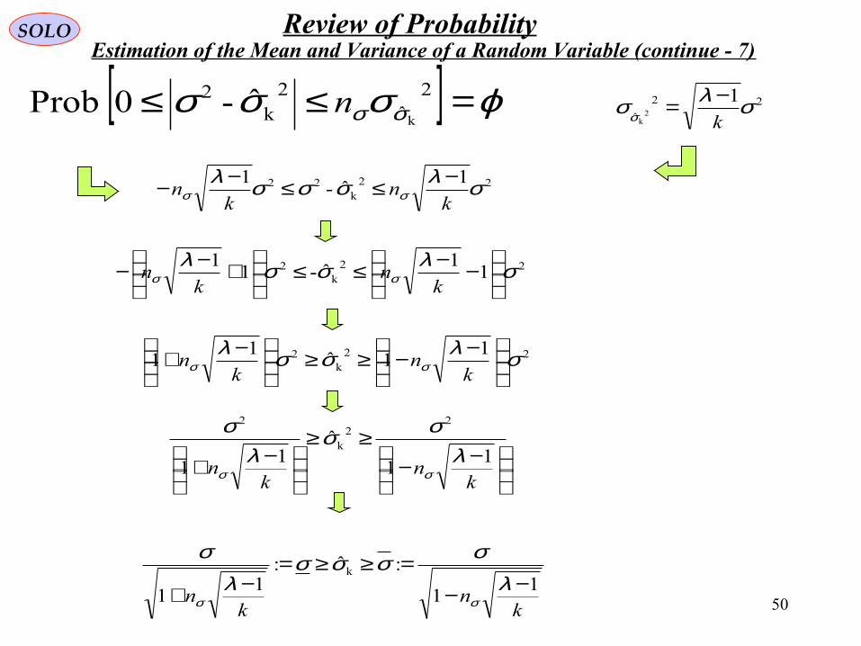
[ ] ϕσσσ σσ =≤≤ 2ˆ
2k
2
kˆ-0Prob n
22k
22 1ˆ-
1 σλσσσλσσ k
nk
n−≤≤−−
22k
2 11
ˆ-11 σλσσλ
σσ
−−≤≤
+−−
kn
kn
22
ˆ
12
kσλσ
σ k
−=
22k
2 11ˆ
11 σλσσλ
σσ
−−≥≥
−+k
nk
n
−−≥≥
−+k
nk
n1
1
ˆ1
1
22
k
2
λσσ
λσ
σσ
kn
kn
11
:ˆ:1
1
k
−−
=≥≥=−+ λ
σσσσλ
σ
σσ

51
SOLO Review of ProbabilityEstimation of the Mean and Variance of a Random Variable (continue - 8)

52
SOLO Review of ProbabilityEstimation of the Mean and Variance of a Random Variable (continue - 9)
53
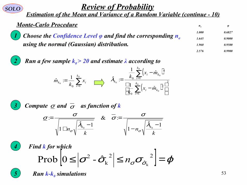
SOLO Review of ProbabilityEstimation of the Mean and Variance of a Random Variable (continue - 10)
kn
kn kk 1ˆ
1
:&1ˆ
1
:
00−
−
=−
+
=λ
σσλ
σσ
σσ
Monte-Carlo Procedure
Choose the Confidence Level φ and find the corresponding nσ
using the normal (Gaussian) distribution.
nσ φ
1.000 0.6827
1.645 0.9000
1.960 0.9500
2.576 0.9900
1
Run a few sample k0 > 20 and estimate λ according to2
( )
( )2
1
2
0
1
4
0
0
0
0
0
0
ˆ1
ˆ1
:ˆ
−
−=
∑
∑
=
=
k
iki
k
iki
k
mxk
mxkλ∑
==
0
010
1:ˆ
k
iik x
km
3 Compute and as function of kσ σ
4 Find k for which
[ ] ϕσσσ σσ =≤≤ 2ˆ
2k
2
kˆ-0Prob n
5 Run k-k0 simulations

54
SOLO Review of ProbabilityEstimation of the Mean and Variance of a Random Variable (continue – 11)
Monte-Carlo Procedure
Choose the Confidence Level φ = 95% that gives the corresponding nσ=1.96.
nσ φ
1.000 0.6827
1.645 0.9000
1.960 0.9500
2.576 0.9900
1
The kurtosis λ = 32
3 Find k for which ϕσλσσ
σ
σ =
−≤≤
2kˆ
22k
2 1ˆ-0Prob
kn
4 Run k>800 simulations
Example:Assume a Gaussian distribution λ = 3
95.02
96.1ˆ-0Prob
2kˆ
22k
2 =
≤≤
σ
σσσk
Assume also that we require also that with probability φ = 95 % 22k
2 1.0ˆ- σσσ ≤
1.02
96.1 =k
800≈k

55
SOLO Review of Probability
Generating Discrete Random Variables
Pseudo-Random Number Generators
• First attempts to generate “random numbers”:- Draw balls out of a stirred urn- Roll dice
• 1927: L.H.C. Tippett published a table of 40,000 digits taken “at random” from census reports.
• 1939: M.G. Kendall and B. Babington-Smith create a mechanical machine to generate random numbers. They published a table of 100,000 digits.
• 1946: J. Von Neumann proposed the “middle square method”.
• 1948: D.H. Lehmer introduced the “linear congruential method”.
• 1955: RAND Corporation published a table of 1,000,000 random digits obtainedfrom electronic noise.
• 1965: M.D. MacLaren and G. Marsaglia proposed to combine two congruentialgenerators.
• 1989: R.S. Wikramaratna proposed the additive congruential method.

56
SOLO Review of Probability
Generating Discrete Random Variables
Pseudo-Random Number Generators
A Random Number represents the value of a random variable uniform distributed on (0,1). Pseudo-Random Numbers constitute a sequence of values, which although are deterministically generated, have all the appearances of being independent uniform distributed on (0,1).One approach
1. Define x0 = integer initial condition or seed
2. Using integers a and m recursively compute
mxax nn modulo1−= mxIntegerxkmaxmkxa nnn <∈+⋅=− ,,,1
Therefore xn takes the values 0,1,…,m-1 and the quantity un=xn/m , called a pseudo-randomnumber is an approximation to the value of uniform (0,1) random variable.
In general the integers a and m should be chose to satisfy three criteria:
1. For any initial seed, the resultant sequence has the “appearance” of being a sequence of independent (0,1) random variables.
2. For any initial seed, the number of variables that can be generated before repetitionbegins is large.
3. The values can be computed efficiently on a digital computer.
Multiplicative congruential method
Return toMonte Carlo Approximation
57
SOLO Review of Probability
Generating Discrete Random Variables
Pseudo-Random Number Generators (continue – 1)
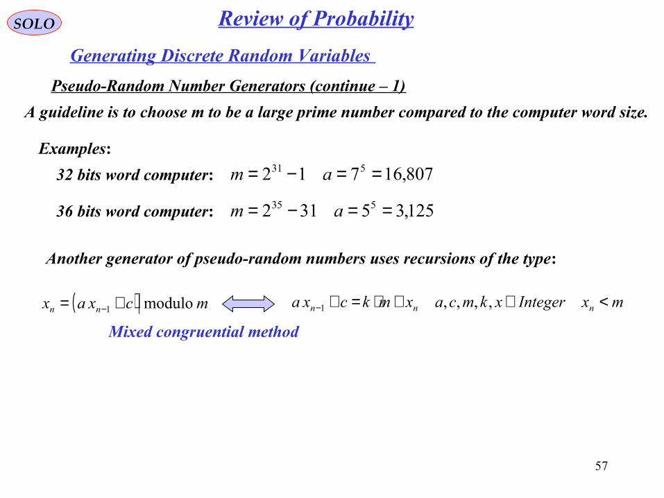
A guideline is to choose m to be a large prime number compared to the computer word size.
Examples:
32 bits word computer: 807,16712 531 ==−= am
125,35312 535 ==−= am36 bits word computer:
Another generator of pseudo-random numbers uses recursions of the type:
( ) mcxax nn modulo1 += − mxIntegerxkmcaxmkcxa nnn <∈+⋅=+− ,,,,1
Mixed congruential method

58
SOLO Review of Probability
Generating Discrete Random Variables
Histograms
Return to Table of Content
A histogram is a graphical display of tabulated frequencies, shown as bars. It shows what proportion of cases fall into each of several categories: it is a form of data binning. The categories are usually specified as non-overlapping intervals of some variable. The categories (bars) must be adjacent. The intervals (or bands, or bins) are generally of the same size.
Histograms are used to plot density of data, and often for density estimation: estimating the probability density function of the underlying variable. The total area of a histogram always equals 1. If the length of the intervals on the x-axis are all 1, then a histogram is identical to a relative frequency plot.
A cumulative histogram is a mapping that counts the cumulative number of observations in all of the bins up to the specified bin. That is, the cumulative histogram Mi of a histogram mi is defined as:
An ordinary and a cumulative histogram of the same data. The data shown is a random sample of 10,000 points from a normal distribution with a mean of 0 and a standard deviation of 1.
Mathematical Definition
∑=
=k
iimn
1
In a more general mathematical sense, a histogram is a mapping mi that counts the number of observations that fall into various disjoint categories (known as bins), whereas the graph of a histogram is merely one way to represent a histogram. Thus, if we let n be the total number of observations and k be the total number of bins, the histogram mi meets the following conditions:
∑=
=i
jji mM
1

59
SOLO Review of Probability
Generating Discrete Random Variables
The Inverse Transform Method
Suppose we want to generate a discrete random variable X having probability density function:
( ) 1,1,0)( ==−= ∑j
jjj pjxxpxp δ
To accomplish this, let generate a random number U that is uniformly distributedover (0,1) and set:
<≤
+<≤<
=
∑∑=
−
=
j
ii
j
iij pUpifx
ppUpifx
pUifx
X
1
1
1
1001
00
j
j
ii
j
iij ppUpPxXP =
<<== ∑∑=
−
= 1
1
1
)(
Since , for any a and b such that 0 < a < b < 1, and U is uniformly distributed P (a ≤ U < b) = b-a, we have:
and so X has the desired distribution.

60
SOLO Review of Probability
Generating Discrete Random Variables
The Inverse Transform Method (continue – 1)
Suppose we want to generate a discrete random variable X having probability density function: ( ) 1,1,0)( ==−= ∑
jjjj pjxxpxp δ
Draw X, N times, from p (x)
Histogram of theResults

61
SOLO Review of Probability
Generating Discrete Random Variables
The Inverse Transform Method (continue – 2)
Generating a Poisson Random Variable: 1,1,0!
)( ===== ∑−
ii
i
i pii
eiXPp λλ
( )1
!
!1
1
1
+=+=
−
+−
+
ii
e
ie
p
pi
i
i
i λλ
λ
λ
λ
Draw X , N times, from Poisson Distribution
Histogram of the Results
62
SOLO Review of Probability
Generating Discrete Random Variables
The Inverse Transform Method (continue – 3)
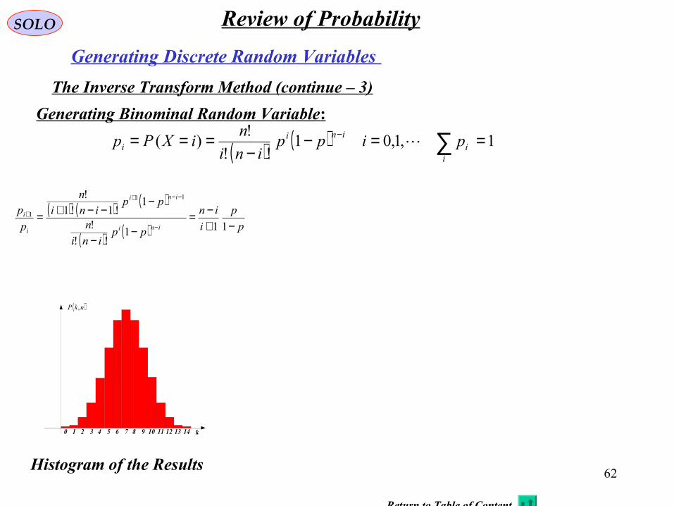
Generating Binominal Random Variable:
( ) ( ) 1,1,01!!
!)( ==−
−=== ∑−
ii
inii pipp
ini
niXPp
( ) ( ) ( )
( ) ( ) p
p
i
in
ppini
n
ppini
n
p
pini
ini
i
i
−+−=
−−
−−−+=
−
−−+
+
111!!
!
1!1!1
! 11
1
Return to Table of Content
0 1 2 3 4 5 6 7 8 9 10 11 12 13 14 k
( )nkP ,
Histogram of the Results

63
SOLO Review of Probability
Generating Discrete Random Variables
The Accaptance-Rejection Technique
Suppose we have an efficient method for simulating a random variable having aprobability density function qj, j ≥0 . We want to use this to obtain a randomvariable that has the probability density function pj, j ≥0 .
Let c be a constant such that: 0.. ≠∀≤ jj
j qtsjcq
p
If such a c exists, it must satisfy: cqcpj
jj
j ≤⇒≤ ∑∑ 1
11
Rejection Method
Step 1: Simulate the value of Y, having probability density function qj.
Step 2: Generate a random number U (that is uniformly distributedover (0,1) ).Step 3: If U < pY/c qY, set X = Y and stop. Otherwise return to Step 1.

64
SOLO Review of Probability
Generating Discrete Random Variables
The Acceptance-Rejection Technique (continue – 1)
Theorem
The random variable X obtained by the rejection method has probability densityfunction P X=i = pi.Proof
Acceptance
,
Acceptance
Acceptance,Acceptance
MethodAcceptance
MethodAcceptance
P
qc
pUiYP
P
iYPiYPiXP i
i
Bayes
≤=======
AcceptanceAcceptanceAcceptance
(0,1) ddistributeuniformlyU
ceindependenby
Pc
p
P
qc
pq
P
qc
pUPiYP
ii
ii
i
i
qi
==
≤==
Summing over all i, yields
Acceptance
1
1
Pc
piXP i
i
i
∑∑ ==
1Acceptance =Pc
ipiXP ==
11
Acceptance ≤=c
P
q.e.d.

65
SOLO Review of Probability
Generating Discrete Random Variables
The Acceptance-Rejection Technique (continue – 2)
Example
Generate a truncated Gaussian using theAccept-Reject method. Consider the case with
( ) [ ]
−∈≈
−
otherwise
xexp
x
0
4,42/2/2
π
Consider the Uniform proposal function
( ) [ ] −∈
≈otherwise
xxq
0
4,48/1
In Figure we can see the results of theAccept-Reject method using N=10,000 samples.

66
SOLO Review of Probability
Generating Continuous Random Variables
The Inverse Transform Algorithm
Let U be a uniform (0,1) random variable. For any continuous distribution function F the random variable X defined by
( )UFX 1−=has distribution F. [ F-1(u) is defined to be that value of x such that F (x) = u ]
Proof
Let Px(x) denote the Probability Distribution Function X=F-1(U)
( ) ( ) xUFPxXPxPx ≤=≤= −1
Since F is a distribution function, it means that F (x) is a monotonic increasing function of x and so the inequality “a ≤ b” is equivalent to the inequality“F (a) ≤ F (b)”, therefore
( ) ( )[ ] ( ) ( )[ ]
( ) ( )
( )( )xFxFUP
xFUFFPxPuniformU
xF
UUFF
x
1,0
10
1
1
≤≤
=
−
=≤=
≤=−
67
SOLO Review of Probability
Importance Sampling
Let Y = (Y1,…,Ym) a vector of random variables having a joint probability densityfunction f (y1,…,ym), and suppose that we are interested in estimating
( )[ ] ( ) ( )∫== mmmmf dydyyyfyyhYYhE 1111 ,,,,,,θ Suppose that a direct generation of the random vector Y so as to compute h (Y) is inefficient possible because (a) is difficult to generate the random vector Y, or
(b) the variance of h (Y) is large, or
(c) both of the above
Suppose that W=(W1,…,Wm) is another random vector, which takes values in thesame domain as Y, and has a joint density function g(w1,…,wm) that can be easily generated. The estimation θ can be expressed as:
( )[ ] ( ) ( )( ) ( ) ( ) ( )
( )
=== ∫ Wg
WfWhEdwdwwwg
wwg
wwfwwhYYhE gmm
m
mmmf
11
1
111 ,,
,,
,,,,,,θ
Therefore, we can estimate θ by generating values of random vector W, and thenusing as the estimator the resulting average of the values h (W) f (W)/ g (W).
Return to Particle Filters

68
SOLO Review of Probability
Monte Carlo Integration
Monte Carlo Method can be used to numerically evaluate multidimensional integrals
( ) ( )∫∫ == xdxgdxdxxxgI mm 11 ,,
To use Monte Carlo we factorize ( ) ( ) ( )xpxfxg ⋅=
( ) ( ) 1&0 =≥ ∫ xdxpxp
in such a way that is interpreted as a Probability Density Function such that( )xp
We assume that we can draw NS samples from ( )xp( )Si Nix ,,1, =
( ) Si Nixpx ,,1~ =
Using Monte Carlo we can approximate ( ) ( )∑=
−≈SN
iS
i Nxxxp1
/δ
( ) ( ) ( ) ( )
( ) ( ) ( )∑∑∫
∫ ∑∫
==
=
=−⋅=
−⋅=≈⋅=
SS
S
S
N
i
i
S
N
i
i
S
N
iS
iN
xfN
xdxxxfN
xdNxxxfIxdxpxfI
11
1
11
/
δ
δ

69
SOLO Review of Probability
Monte Carlo Integration
we draw NS samples from ( )xp( )Si Nix ,,1, =
( ) Si Nixpx ,,1~ =
( ) ( ) ( )∑∫=
=≈⋅=S
S
N
i
i
SN xf
NIxdxpxfI
1
1
If the samples are independent, then INS is an unbiased estimate of I.
ix
According to the Law of Large Numbers INS will almost surely converge to I:
IIsa
NN
SS
..
∞→→
( )[ ] ( ) ∞<−= ∫ xdxpIxff22 :σIf the variance of is finite; i.e.:( )xf
then the Central Limit Theorem holds and the estimation error converges indistribution to a Normal Distribution:
( ) ( )2,0~lim fNSN
IINS
S
σN−∞→
The error of the MC estimate, e = INS – I, is of the order of O (NS
-1/2), meaning
that the rate of convergence of the estimate is independent of the dimension ofthe integrand.
Numerical Integration of and ( )kk xzp |( )1| −kk xxp
Return to Particle Filters

70
SOLO Review of Probability
Existence Theorems
Existence Theorem 3
Given a function S (ω)= S (-ω) or, equivalently, a positive-defined function R (τ),(R (τ) = R (-τ), and R (0)=max R (τ), for all τ ), we can find a stochastic process x (t)having S (ω) as its power spectrum or R (τ) as its autocorrelation.
Proof of Existence Theorem 3
Define ( ) ( ) ( ) ( ) ( )ωπ
ωπ
ωωωωπ
−=−=== ∫+∞
∞−
fa
S
a
SfdSa
222 :&
1:
Since , according to Existence Theorem 1,
we can find a random variable ω with the even density function f (ω), andprobability density function
( ) ( ) 1&0 =≥ ∫+∞
∞−
ωωω dff
( ) ( )∫∞−
=ω
ττω dfP :
We now form the process , where is a random variableuniform distributed in the interval (-π,+π) and independent of ω.
( ) ( )ϑω += tatx cos: ϑ

71
SOLO Review of Probability
Existence Theorems
Existence Theorem 3
Proof of Existence Theorem 3 (continue – 1)
Since is uniform distributed in the interval (-π,+π) and independent of ω,its spectrum is
( ) ( ) ( ) ( ) ( ) 0sinsincoscos00
,
=−=ϑωϑω ϑωϑω
ϑωEtEaEtEatxE
tindependen
ϑ
( ) ( )ϖπ
ϖπϖπϖπ
ϑπ
ϖπϖπϖπ
π
ϑϖπ
π
ϑϖϑϖϑϑ
sin
2
1
2
1
2
1 =−====−+
−
+
−∫ j
ee
j
edeeES
jjjjj
or ( ) ( ) ( )ϖπ
ϖπϑϖϑϖ ϑϑϑϖ
ϑsin
sincos =+= EjEeE j
1=ϖ 1=ϖ
( ) ( ) ( ) ( )[ ]
( ) ( )[ ]
( ) ( )[ ] ( ) ( )[ ] ( ) 02022,
22
2
2sin2sin2
2cos2cos2
cos2
22cos2
cos2
coscos
ϑτωϑτωτω
ϑτωτω
ϑτωϑωτ
ϑωϑωω
ϑωEtE
aEtE
aE
a
tEa
Ea
ttEatxtxE
tindependen
+−++=
+++=
+++=+
2=ϖ 2=ϖ
Given a function S (ω)= S (-ω) or, equivalently, a positive-defined function R (τ),(R (τ) = R (-τ), and R (0)=max R (τ), for all τ ), we can find a stochastic process x (t)having S (ω) as its power spectrum or R (τ) as its autocorrelation.

72
SOLO Review of Probability
Existence Theorems
Existence Theorem 3
Proof of Existence Theorem 3 (continue – 2)
( ) 0=txE
( ) ( ) ( ) ( ) ( ) ( )τωωτωτωτ ω xRdfa
Ea
txtxE ===+ ∫+∞
∞−
cos2
cos2
22
( ) ( )ϑω += tatx cos:We have
Because of those two properties x (t) is wide-sense stationary with a power spectrumgiven by:
( ) ( ) ( ) ( )[ ]( ) ( )
( ) ( )∫∫+∞
∞−
−=+∞
∞−
=−= ττωτττωτωτωττ
dRdjRS x
RR
xx
xx
cossincos
( ) ( ) ( ) ( )[ ]( ) ( )
( ) ( )∫∫+∞
∞−
−=+∞
∞−
=+= ωτωωπ
ωτωτωωπ
τωω
dSdjSR x
SS
xx
xx
cos2
1sincos
2
1
Therefore ( ) ( )ωπω faSx2=
q.e.d.
Fourier InverseFourier
( ) ( )∫+ ∞
∞−
= ωωτω dfa
cos2
2
f (ω) definition
( )ωS=
Given a function S (ω)= S (-ω) or, equivalently, a positive-defined function R (τ),(R (τ) = R (-τ), and R (0)=max R (τ), for all τ ), we can find a stochastic process x (t)having S (ω) as its power spectrum or R (τ) as its autocorrelation.

73
SOLO
Markov Processes
A Markov Process is defined by:
Andrei AndreevichMarkov
1856 - 1922
( ) ( )( ) ( ) ( )( ) 111 ,|,,,|, tttxtxptxtxp >∀ΩΩ=≤ΩΩ ττ
i.e. the Random Process, the past up to any time t1 is fully defined by the process at t1.
Examples of Markov Processes:
1. Continuous Dynamic System( ) ( )( ) ( )vuxthtz
wuxtftx
,,,
,,,
==
2. Discrete Dynamic System
( ) ( )( ) ( )kkkkk
kkkkk
vuxthtz
wuxtftx
,,,
,,, 1111
== −−−−
x - state space vector (n x 1)u - input vector (m x 1)
- measurement vector (p x 1)z
v - white measurement noise vector (p x 1)
- white input noise vector (n x 1)w
Recursive Bayesian Estimation

74
Recursive Bayesian EstimationSOLO
Using this property we obtain:
( ) ( )1021 |,,,| −−− = kkkkk xxpxxxxp
Markov Processes
( ) ( )( )
( )
( ) ( )( )
( )
( ) ( )∏=
−
−−−−
−−−−−−
=
=
=
−−
−
k
iii
k
xxp
kkkk
kk
xxp
kkkkkk
xxpxp
xxpxxxpxxp
xxxpxxxxpxxxxp
kk
kk
110
02
|
0211
021
|
021021
|
,,,,||
,,,,,,|,,,,
21
1
Markov Process:
Table of Content
the present discrete state probability depends only on the previous state.
The Markov Process is defined if we know p (x0) and p(xi|xi-1) for each i.

75
Recursive Bayesian EstimationSOLO
In a Markovian system the probability of the current true state depends only on the previous state, and is independent of the other earlier states
( ) ( )1021 |,,,| −−− = kkkkk xxpxxxxp
Similarly the measurements at the k-th time-step is dependent upon the current true state, so is conditionally independent of all other earlier states, given the current state
( ) ( )kkkkk xzpxxxzp |,,,| 01 =−
( ) ( ) ( ) ( ) ( )kkkkkkkk zpzxpxpxzpxzp ||, ==
From the definition of the Markovian system (see Figure) p (xk|xk-1) is defined byf and the statistics of x and w and p (zk|xk) is defined by h and statistics of x and v.
kx1−kx
kz1−kz
0x 1x 2x
1z 2z kZ :11:1 −kZ
( )111 ,, −−− kkk wuxf
( )kk vxh ,
Markov Processes
( )000 ,, wuxf
( )11,vxh
( )111 ,, wuxf
( )22 ,vxh
Hidden States
Measurements
76
Recursive Bayesian EstimationSOLO
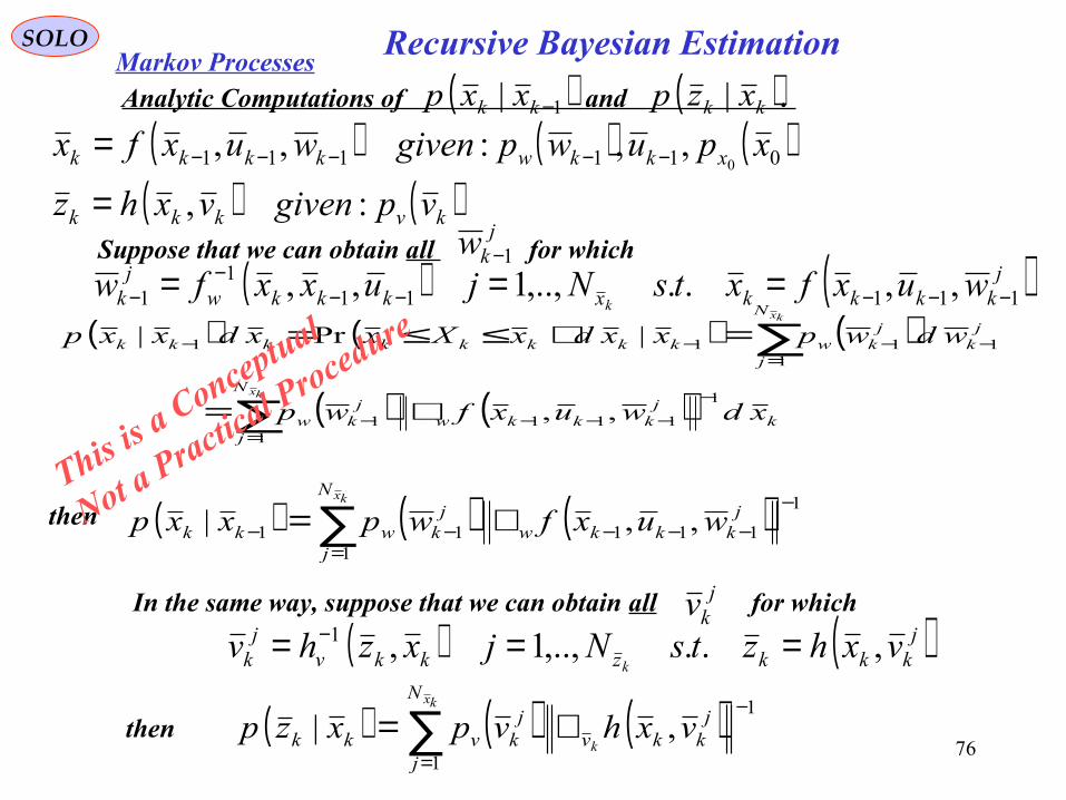
( ) ( ) ( )( ) ( )kvkkk
xkkwkkkk
vpgivenvxhz
xpuwpgivenwuxfx
:,
,,:,, 011111 0
=
= −−−−−
Markov Processes
( ) ( )jkkkkxkkkw
jk wuxfxtsNjuxxfw
k 111111
1 ,,..,..,1,, −−−−−−
− ===Suppose that we can obtain all for which
jkw 1−
( ) ( ) ( )∑=
−
−−−−− ∇=kx
N
j
jkkkw
jkwkk wuxfwpxxp
1
1
11111 ,,|then
( ) ( ) ( )∑=
−∇=
kx
k
N
j
jkkv
jkvkk vxhvpxzp
1
1,|
( ) ( )jkkkzkkvjk vxhztsNjxzhv
k,..,..,1,1 === −
In the same way, suppose that we can obtain all for whichjkv
then
( ) ( ) ( )
( ) ( )∑
∑
=
−
−−−−
=−−−−
∇=
=+≤≤=
kx
kx
N
jk
jkkkw
jkw
N
j
jk
jkwkkkkkkkk
xdwuxfwp
wdwpxxdxXxxdxxp
1
1
1111
11111
,,
|Pr|
This is a
Conceptual
Not a Practical Procedure
Analytic Computations of and . ( )kk xzp |( )1| −kk xxp

77
Recursive Bayesian EstimationSOLO
( ) ( ) ( )( ) ( )kvkkk
xkkwkkkk
vpgivenvxhz
xpuwpgivenwuxfx
:
,,:, 011111 0
+=
+= −−−−−
kx1−kx
kz1−kz
( ) 111, −−− + kkk wuxf
( ) kk vxh +
Markov Processes
( ) ( )[ ]111 ,| −−− −= kkkwkk uxfxpxxptherefore
( ) ( )[ ]kkvkk xhzpxzp −=|and
For additive noise
we have( )
( )kkk
kkkk
xhzv
uxfxw
−=−= −−− 111 ,
Analytic Computations of and (continue – 1) ( )kk xzp |( )1| −kk xxp

78
SOLO
( )( )kkk
kkk
vxhz
wxfx
,
, 11
== −−
kk vw &1− are system and measurement white-noise sequencesindependent of past and current states and on each other andhaving known P.D.F.s ( ) ( )kk vpwp &1−
We want to compute p (xk|Z1:k) recursively, assuming knowledge of p(xk-1|Z1:k-1) in two stages, prediction (before) and update (after measurement)
( ) ( )( ) ( )∫ −−−−− −= 11111 ,| kkkkkkk wdwpwxfxxxp δWe need to evaluate the following integrals:
( ) ( )( ) ( )∫ −= kkkkkkk vdvpvxhzxzp ,| δ
We use the numeric Monte Carlo Method to evaluate the integrals:
Generate (Draw): ( ) ( ) Skikk
ik Nivpvwpw ,,1~&~ 11 =−−
( ) ( )( ) S
N
i
ik
ik
ikkk Nwxfxxxp
S
∑=
−−− −≈1
111 /,| δ
( ) ( )( ) S
N
i
ik
ik
ikkk Nvxhzxzp
S
∑=
−≈1
/,| δor
( ) ( ) ( ) S
N
i
ikkkk
ik
ik
ik Nxxxxpwxfx
S
∑=
−−− −≈→=1
111 /|, δ
( ) ( ) ( ) S
N
i
ikkkk
ik
ik
ik Nzzxzpvxhz
S
∑=
−≈→=1
/|, δ
Analytic solutions for those integralequations do not exist in the generalcase.
Recursive Bayesian EstimationNumerical Computations of and .( )kk xzp |( )1| −kk xxpMarkov Processes
Prediction (before measurement) ( ) ( ) ( )∫ −−−−− = 11:1111:1 ||| kkkkkkk xdZxpxxpZxp1Update (after measurement)
( ) ( )( ) ( ) ( )
( )
( ) ( )( )
( ) ( )( ) ( )∫ −
−
−
−
=− ===
kkkkk
kkkk
kk
kkkkBayes
bp
apabpbap
kkkkkxdZxpxzp
Zxpxzp
Zzp
ZxpxzpZzxpZxp
1:1
1:1
1:1
1:1
||
1:1:1||
||
|
||,||
2
79
Recursive Bayesian EstimationSOLO
( ) ( ) ( )( ) ( )kvkkk
xkkwkkkk
vpgivenvxhz
xpuwpgivenwuxfx
:,
,,:,, 011111 0
=
= −−−−−
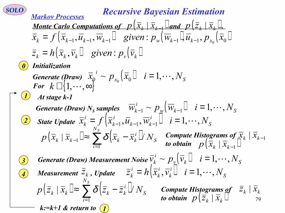
Markov ProcessesMonte Carlo Computations of and . ( )kk xzp |( )1| −kk xxp
Generate (Draw) ( ) Sxi Nixpx ,,1~ 00 0
=For ∞∈ ,,1 k
Initialization0
1 At stage k-1
Generate (Draw) NS samples ( ) Skwik Niwpw ,,1~ 11 =−−
2 State Update ( ) Sikk
ik
ik Niwuxfx ,,1,, 111 == −−−
3 Generate (Draw) Measurement Noise ( ) Skvik Nivpv ,,1~ =
k:=k+1 & return to 1
Compute Histograms of to obtain ( )kk xzp |
kk xz |
( ) ( )∑=
− −≈SN
iS
ikkkk Nxxxxp
11 /| δ
( ) ( )∑=
−≈SN
iS
ikkkk Nzzxzp
1
/| δ
Compute Histograms of to obtain
1| −kk xx( )1| −kk xxp
4 Measurement , Update ( ) Sik
ik
ik Nivxhz ,,1, ==kz
SOLO
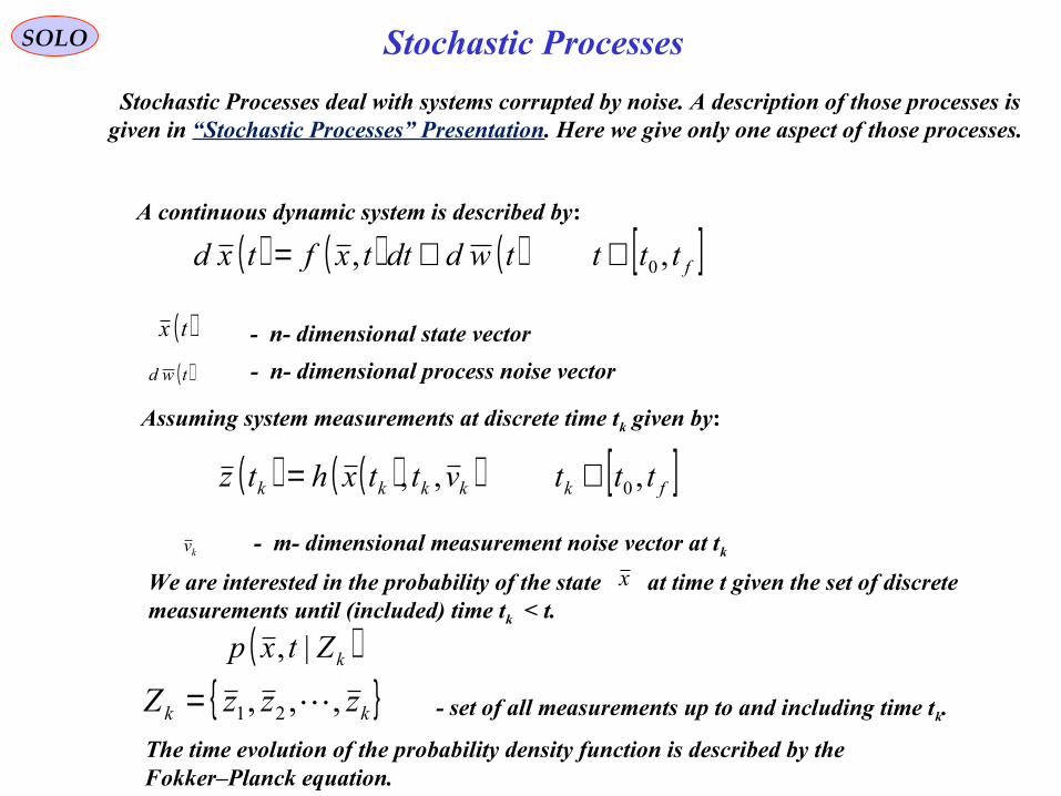
Stochastic Processes deal with systems corrupted by noise. A description of those processes is given in “Stochastic Processes” Presentation. Here we give only one aspect of those processes.
( ) ( ) ( ) [ ]fttttwddttxftxd ,, 0∈+=A continuous dynamic system is described by:
Stochastic Processes
( )tx - n- dimensional state vector
( )twd - n- dimensional process noise vector
Assuming system measurements at discrete time tk given by:
( ) ( )( ) [ ]fkkkkk tttvttxhtz ,,, 0∈=
kv - m- dimensional measurement noise vector at tk
We are interested in the probability of the state at time t given the set of discrete measurements until (included) time tk < t.
x
( )kZtxp |,
kk zzzZ ,,, 21 = - set of all measurements up to and including time tk.
The time evolution of the probability density function is described by the Fokker–Planck equation.
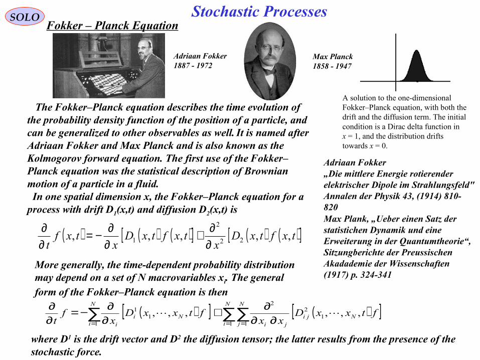
A solution to the one-dimensional Fokker–Planck equation, with both the drift and the diffusion term. The initial condition is a Dirac delta function in x = 1, and the distribution drifts towards x = 0.
The Fokker–Planck equation describes the time evolution of the probability density function of the position of a particle, and can be generalized to other observables as well. It is named after Adriaan Fokker and Max Planck and is also known as the Kolmogorov forward equation. The first use of the Fokker–Planck equation was the statistical description of Brownian motion of a particle in a fluid. In one spatial dimension x, the Fokker–Planck equation for a process with drift D1(x,t) and diffusion D2(x,t) is
More generally, the time-dependent probability distribution may depend on a set of N macrovariables xi. The general form of the Fokker–Planck equation is then
where D1 is the drift vector and D2 the diffusion tensor; the latter results from the presence of the stochastic force.
Fokker – Planck Equation
Adriaan Fokker 1887 - 1972
Max Planck1858 - 1947
SOLO
Adriaan Fokker„Die mittlere Energie rotierender elektrischer Dipole im Strahlungsfeld" Annalen der Physik 43, (1914) 810-820 Max Plank, „Ueber einen Satz der statistichen Dynamik und eine Erweiterung in der Quantumtheorie“, Sitzungberichte der Preussischen Akadademie der Wissenschaften (1917) p. 324-341
Stochastic Processes
( ) ( ) ( )[ ] ( ) ( )[ ]txftxDx
txftxDx
txft
,,,,, 22
2
1 ∂∂+
∂∂−=
∂∂
( )[ ] ( )[ ]∑∑∑= == ∂∂
∂+∂∂−=
∂∂ N
i
N
jNji
ji
N
iNi
i
ftxxDxx
ftxxDx
ft 1 1
12
2
11
1 ,,,,,,

Fokker – Planck Equation (continue – 1)
The Fokker–Planck equation can be used for computing the probability densities of stochastic differential equations.
where is the state and is a standard M-dimensional Wiener process. If the initial probability distribution is , then the probability distribution of the stateis given by the Fokker – Planck Equation with the drift and diffusion terms:
Similarly, a Fokker–Planck equation can be derived for Stratonovich stochastic differential equations. In this case, noise-induced drift terms appear if the noise strength is state-dependent.
SOLO
Consider the Itô stochastic differential equation:
( ) ( ) ( )[ ] ( ) ( )[ ]txftxDx
txftxDx
txft
,,,,, 22
2
1 ∂∂+
∂∂−=
∂∂

Fokker – Planck Equation (continue – 2)
Derivation of the Fokker–Planck Equation
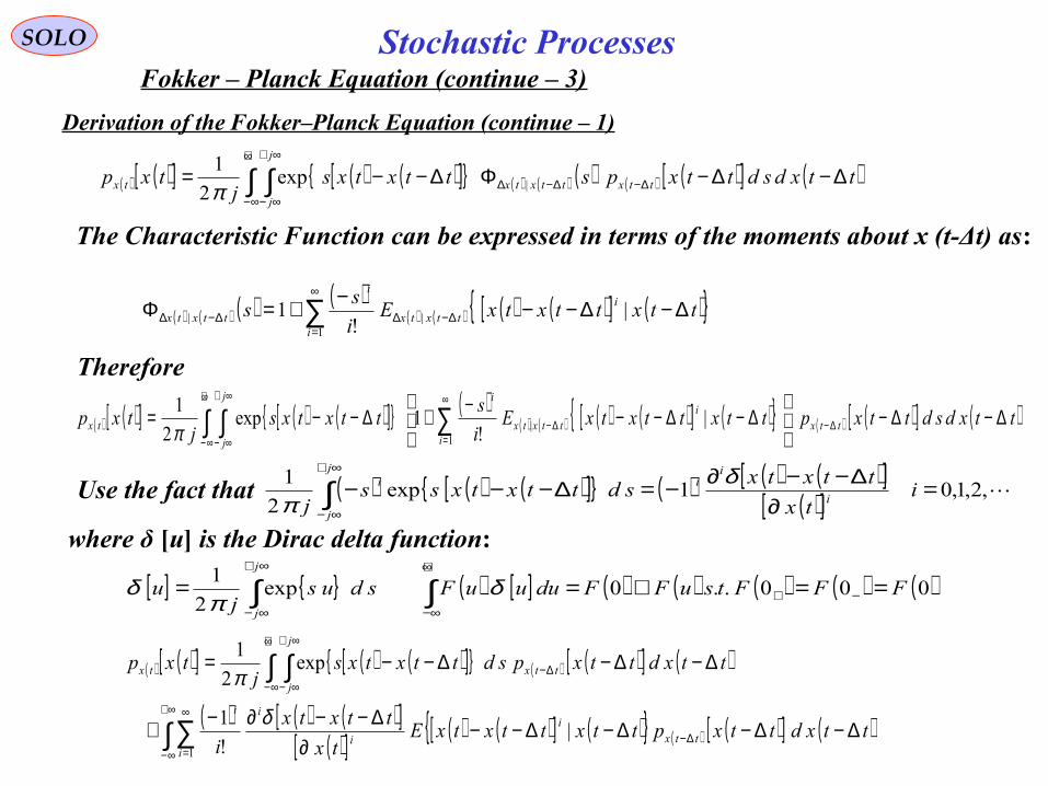
SOLO
Start with ( ) ( ) ( )11|1, 111|, −−− −−−
= kxkkxxkkxx xpxxpxxpkkkkk
and ( ) ( ) ( ) ( )∫∫+∞
∞−−−−
+∞
∞−−− −−−
== 111|11, 111|, kkxkkxxkkkxxkx xdxpxxpxdxxpxp
kkkkkk
define ( ) ( )ttxxtxxttttt kkkk ∆−==∆−== −− 11 ,,,
( ) ( )[ ] ( ) ( ) ( ) ( )[ ] ( ) ( )[ ] ( )∫+∞
∞−∆−∆− ∆−∆−∆−= ttxdttxpttxtxptxp ttxttxtxtx ||
Let use the Characteristic Function of
( ) ( ) ( ) ( ) ( )[ ] ( ) ( ) ( ) ( )[ ] ( ) ( ) ( ) ( )ttxtxtxtxdttxtxpttxtxss ttxtxttxtx ∆−−=∆∆−∆−−−=Φ ∫+∞
∞−∆−∆−∆ |exp: ||
( ) ( ) ( ) ( )[ ]ttxtxp ttxtx ∆−∆− ||
The inverse transform is ( ) ( ) ( ) ( )[ ] ( ) ( )[ ] ( ) ( ) ( )∫∞+
∞−∆−∆∆− Φ∆−−=∆−
j
j
ttxtxttxtx sdsttxtxsj
ttxtxp || exp2
1|
π
Using Chapman-Kolmogorov Equation we obtain:
( ) ( )[ ] ( ) ( )[ ] ( ) ( ) ( )
( ) ( ) ( ) ( )[ ]
( ) ( )[ ] ( )
( ) ( )[ ] ( ) ( ) ( ) ( ) ( )[ ] ( )ttxdsdttxpsttxtxsj
ttxdttxpsdsttxtxsj
txp
j
j
ttxttxtx
ttx
ttxtxp
j
j
ttxtxtx
ttxtx
∆−∆−Φ∆−−=
∆−∆−Φ∆−−=
∫ ∫
∫ ∫
∞+
∞−
∞+
∞−∆−∆−∆
+∞
∞−∆−
∆−
∞+
∞−∆−∆
∆−
|
|
|
exp2
1
exp2
1
|
π
π
Stochastic Processes
Fokker – Planck Equation (continue – 3)
Derivation of the Fokker–Planck Equation (continue – 1)
SOLO
The Characteristic Function can be expressed in terms of the moments about x (t-Δt) as:
( ) ( )[ ] ( ) ( )[ ] ( ) ( ) ( ) ( ) ( )[ ] ( )ttxdsdttxpsttxtxsj
txpj
j
ttxttxtxtx ∆−∆−Φ∆−−= ∫ ∫+∞
∞−
∞+
∞−∆−∆−∆ |exp
2
1
π
( ) ( ) ( ) ( )( ) ( ) ( ) ( )[ ] ( ) ∑
∞
=∆−∆∆−∆ ∆−∆−−−+=Φ
1|| |
!1
i
ittxtx
i
ttxtx ttxttxtxEi
ss
Therefore
( ) ( )[ ] ( ) ( )[ ] ( )( ) ( ) ( ) ( )[ ] ( ) ( ) ( )[ ] ( )ttxdsdttxpttxttxtxE
i
sttxtxs
jtxp
j
j
ttxi
ittxtx
i
tx ∆−∆−
∆−∆−−−+∆−−= ∫ ∫ ∑+∞
∞−
∞+
∞−∆−
∞
=∆−
1| |
!1exp
2
1
π
Use the fact that ( ) ( ) ( )[ ] ( ) ( ) ( )[ ]( )[ ] ,2,1,01exp
2
1 =∂
∆−−∂−=∆−−−∫∞+
∞−
itx
ttxtxsdttxtxss
j i
ii
j
j
i δπ
( ) ( )[ ] ( ) ( )[ ] ( ) ( )[ ] ( )
( ) ( ) ( )[ ]( )[ ] ( ) ( )[ ] ( ) ( ) ( )[ ] ( )∫∑
∫ ∫∞+
∞−
∞
=∆−
+∞
∞−∆−
∞+
∞−
∆−∆−∆−∆−−∂
∆−−∂−+
∆−∆−∆−−=
1
|!
1
exp2
1
ittx
i
i
ii
ttx
j
j
tx
ttxdttxpttxttxtxEtx
ttxtx
i
ttxdttxpsdttxtxsj
txp
δ
π
where δ [u] is the Dirac delta function:
[ ] ( ) [ ] ( ) ( ) ( ) ( ) ( )000..0exp2
1FFFtsuFFduuuFsdus
ju
j
j
==∀== −+
+∞
∞−
∞+
∞−∫∫ δ
πδ
Stochastic Processes

Fokker – Planck Equation (continue – 4)
Derivation of the Fokker–Planck Equation (continue – 2)
SOLO
[ ] ( ) ( ) [ ] ( ) ( ) ( ) ( ) ( )afafaftsufufduuaufsduasj
uaau
j
j
==∀=−−=− −+=
+∞
∞−
∞+
∞−∫∫ ..exp
2
1 δπ
δ
[ ] ( ) ( ) ( ) ( ) ( ) ∫∫∫∞+
∞−
∞+
∞−
∞+
∞−
=→=−−=−j
j
j
j
j
j
sdussFsj
ufdu
dsdussF
jufsduass
jua
ud
dexp
2
1exp
2
1exp
2
1
πππδ
( ) [ ] ( ) ( ) ( ) ( )
( ) ( ) ( )au
j
j
j
j
j
j
j
j
ud
ufdsdsFass
jsdduusufass
j
sdduuasufsj
dusduassj
ufduuaud
duf
=
∞+
∞−
∞+
∞−
∞+
∞−
∞+
∞−
+∞
∞−
+∞
∞−
∞+
∞−
+∞
∞−
−=−=−−=
−−=−−=−
∫∫ ∫
∫ ∫∫ ∫∫
exp2
1expexp
2
1
exp2
1exp
2
1
ππ
ππδ
[ ] ( ) ( ) ( ) ( ) ( ) ( ) ∫∫∫∞+
∞−
∞+
∞−
∞+
∞−
=→=−−=−j
j
ii
ij
j
j
j
ii
i
i
sdussFsj
ufdu
dsdussF
jufsduass
jua
ud
dexp
2
1exp
2
1exp
2
1
πππδ
( ) [ ] ( ) ( ) ( ) ( ) ( ) ( )
( ) ( ) ( ) ( ) ( ) ( )au
i
ii
j
j
iij
j
ii
j
j
iij
j
ii
i
i
ud
ufdsdassFs
jsdduusufass
j
sdduuasufsj
dusduassj
ufduuaud
duf
=
−=−=−−=
−−=−−=−
∫∫ ∫
∫ ∫∫ ∫∫∞+
∞−
∞+
∞−
∞+
∞−
∞+
∞−
+∞
∞−
+∞
∞−
∞+
∞−
+∞
∞−
1exp2
1expexp
2
1
exp2
1exp
2
1
ππ
ππδ
Useful results related to integrals involving Delta (Dirac) function
Stochastic Processes
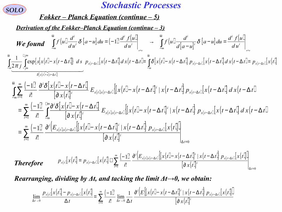
Fokker – Planck Equation (continue – 5)
Derivation of the Fokker–Planck Equation (continue – 3)
SOLO
( ) ( )[ ]
( ) ( )[ ]
( ) ( )[ ] ( ) ( ) ( )[ ] ( ) ( )[ ] ( ) ( ) ( )[ ]txpttxdttxpttxtxttxdttxpsdttxtxsj ttxttxttx
ttxtx
j
j
∆−
+∞
∞−∆−
+∞
∞−∆−
∆−−
∞+
∞−
=∆−∆−∆−−=∆−∆−∆−− ∫∫ ∫ δπ
δ
exp2
1
( ) ( ) ( )[ ]( )[ ] ( ) ( ) ( ) ( )[ ] ( ) ( ) ( )[ ] ( )
( ) ( ) ( )[ ]( )[ ] ( ) ( ) ( ) ( )[ ] ( ) ( ) ( )[ ] ( )
( ) ( ) ( ) ( ) ( )[ ] ( ) ( ) ( )[ ]( )( )[ ]∑
∑ ∫
∫∑
∞
==∆
∆−∆−
∞
=
∞+
∞−∆−∆−
+∞
∞−
∞
=∆−∆−
∂∆−∆−−∂−=
∆−∆−∆−∆−−∂
∆−−∂−=
∆−∆−∆−∆−−∂
∆−−∂−
10
|
1|
1|
|
!
1
|!
1
|!
1
it
i
ttxi
ttxtxii
ittx
ittxtxi
ii
ittx
ittxtxi
ii
tx
txpttxttxtxE
i
ttxdttxpttxttxtxEtx
ttxtx
i
ttxdttxpttxttxtxEtx
ttxtx
i
δ
δ
( ) [ ] ( ) ( ) ( ) [ ] [ ] ( )auau
i
i
i
i
i
ii
i
i
ud
ufdduua
uad
duf
ud
ufdduua
ud
duf
==
=−−
→−=− ∫∫+∞
∞−
+∞
∞−
δδ 1We found
( ) ( )[ ] ( ) ( )[ ] ( ) ( ) ( ) ( ) ( )[ ] ( ) ( ) ( )[ ]( )( )[ ]∑
∞
==∆
∆−∆−∆− ∂
∆−∆−−∂−+=1
0
| |
!
1
it
i
ttxi
ttxtxii
ttxtxtx
txpttxttxtxE
itxptxp
( ) ( )[ ] ( ) ( )[ ] ( ) ( ) ( )[ ] ( ) ( ) ( )[ ]( )( )[ ]∑
∞
=
∆−
→∆
∆−
→∆ ∂∆−∆−−∂
∆−=
∆−
100
|1lim
!
1lim
ii
ttxii
t
ittxtx
t tx
txpttxttxtxE
tit
txptxp
Therefore
Rearranging, dividing by Δt, and tacking the limit Δt→0, we obtain:
Stochastic Processes

Fokker – Planck Equation (continue – 6)
Derivation of the Fokker–Planck Equation (continue – 4)
SOLO
We found ( ) ( )[ ] ( ) ( )[ ] ( ) ( ) ( ) ( ) ( )[ ] ( ) ( ) ( )[ ]( )( )[ ]∑
∞
=
∆−∆−
→∆
∆−
→∆ ∂∆−∆−−∂
∆−=
∆−
1
|
00
|1lim
!
1lim
ii
ttxi
ttxtxi
t
ittxtx
t tx
txpttxttxtxE
tit
txptxp
Define: ( ) ( )[ ] ( ) ( ) ( ) ( )[ ] ( ) t
ttxttxtxEtxtxm
ittxtx
t
i
∆∆−∆−−
=− ∆−
→∆−
|lim: |
0
Therefore ( ) ( )[ ] ( ) ( ) ( )[ ] ( ) ( )[ ]( )( )[ ]∑
∞
=
−
∂−∂−=
∂∂
1 !
1
ii
txiii
tx
tx
txptxtxm
it
txp
( ) ( )ttxtxt
∆−=→∆−
0lim: and:
This equation is called the Stochastic Equation or Kinetic Equation.
It is a partial differential equation that we must solve, with the initial condition:
( ) ( )[ ] ( )[ ]000 0 txptxp tx ===
Stochastic Processes

Fokker – Planck Equation (continue – 7)
Derivation of the Fokker–Planck Equation (continue – 5)
SOLO
We want to find px(t) [x(t)] where x(t) is the solution of
( ) ( ) ( ) [ ]fg ttttntxfdt
txd,, 0∈+=
( ) 0: == tnEn gg
( )tng
( ) ( )[ ] ( ) ( )[ ] ( ) ( )τδττ −=−− ttQnntntnE gggg ˆˆ
Wiener (Gauss) Process
( ) ( )[ ] ( ) ( )[ ] ( ) [ ] ( ) [ ] ( )tQnEtxnEt
ttxttxtxEtxtxm gg
t===
∆∆−∆−−=−
→∆−22
2
2
0
2 ||
lim:
( ) ( )[ ] ( ) ( )[ ] ( ) ( ) ( ) ( ) ( ) ( )txfnEtxftxtd
txdE
t
ttxttxtxEtxtxm g
t,,|
|lim:
0
0
1 =+=
=
∆∆−∆−−=−
→∆−
( ) ( )[ ] ( ) ( )[ ] ( ) 20
|lim:
0>=
∆∆−∆−−=−
→∆− it
ttxttxtxEtxtxm
i
t
i
Therefore we obtain:
( ) ( )[ ] ( )[ ] ( ) ( )[ ]( )( ) ( ) ( ) ( )[ ]
( )[ ] 2
2
2
1,
tx
txptQ
tx
txpttxf
t
txp txtxtx
∂∂
+∂
∂−=
∂∂
Stochastic Processes
Fokker–Planck Equation
Return to Daum

89
Recursive Bayesian EstimationSOLO
Given a nonlinear discrete stochastic Markovian system we want to use k discretemeasurements Z1:k=z1,z2,…,zk to estimate the hidden state xk. For this we want tocompute the probability of xk given all the measurements Z1:k=z1,z2,…,zk .
If we know p ( xk| Z1:k ) then xk is estimated using:
( )∫== kkkkkkkk xdZxpxZxEx :1:1| ||:ˆ
( ) ( ) ( ) ( ) ( )∫ −−=−−= kkkT
kkkkkT
kkkkkk xdZxpxxxxZxxxxEP :1:1| |ˆˆ|ˆˆor more general we can compute all moments of the probability distribution p ( xk| Z1:k ):
( ) ( ) ( )∫= kkkkkk xdZxpxgZxgE :1:1 ||
Bayesian Estimation IntroductionProblem:Estimate the hiddenStates of aNon-linear DynamicStochastic Systemfrom NoisyMeasurements.
kx1−kx
kz1−kz
0x 1x 2x
1z 2z kZ :11:1 −kZ
( )11, −− kk wxf
( )kk vxh ,
( )00 ,wxf
( )11,vxh
( )11,wxf
( )22 ,vxh
The knowledge of p ( xk| Z1:k ) allows also the computation of Maximum a Posteriori(MAP) estimate using: ( )kk
x
MAPkk Zxpx
k:1| |maxargˆ =
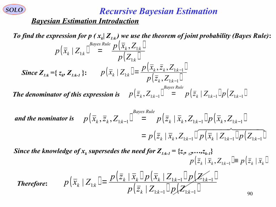
90
Recursive Bayesian EstimationSOLO
To find the expression for p ( xk| Z1:k ) we use the theorem of joint probability (Bayes Rule):
( ) ( )( )k
kkRuleBayes
kk Zp
ZxpZxp
:1
:1:1
,| =
Since Z1:k = zk, Z1:k-1 : ( ) ( )( )1:1
1:1:1 ,
,,|
−
−=kk
kkkkk Zzp
ZzxpZxp
The denominator of this expression is
( ) ( ) ( )1:11:11:1 ,,|,, −−− = kkkkk
RuleBayes
kkk ZxpZxzpZzxp
( ) ( ) ( )
1:11:11:1 |,| −−−= kkkkkk ZpZxpZxzp
Since the knowledge of xk supersedes the need for Z1:k-1 = z1, z2,…,zk-1
( ) ( )kkkkk xzpZxzp |,| 1:1 ≡−
( ) ( ) ( ) ( )( ) ( )1:11:1
1:11:1:1 |
|||
−−
−−=kkk
kkkkkkk ZpZzp
ZpZxpxzpZxpTherefore:
( ) ( ) ( )1:11:11:1 |, −−− = kkk
RuleBayes
kk ZpZzpZzp
and the nominator is
Bayesian Estimation Introduction

91
Recursive Bayesian EstimationSOLO
The final result is: ( ) ( ) ( )
( )1:1
1:1:1 |
|||
−
−=kk
kkkkkk Zzp
ZxpxzpZxp
Therefore:
Since p ( xk| Z1:k ) is a probability distribution it must satisfy:
( ) ( ) ( )( )
( ) ( )( )∫ ∫∫
−
−
−
− ===1:1
1:1
1:1
1:1:1 |
||
|
|||1
kk
kkkkk
kkk
kkkkkkk Zzp
xdZxpxzpxd
Zzp
ZxpxzpxdZxp
( ) 1| :1 =∫ kkk xdZxp
( ) ( ) ( )∫ −− = kkkkkkk xdZxpxzpZzp 1:11:1 |||
( ) ( ) ( )( ) ( )∫ −
−=kkkkk
kkkkkk
xdZxpxzp
ZxpxzpZxp
1:1
1:1:1
||
|||
and:
This is a recursive relation that needs the value of p (xk|Z1:k-1), assuming thatp (zk|xk) is obtained from the Markovian system definition ( zk = h (xk,vk) ).
Bayesian Estimation Introduction
kx1−kx
kz1−kz
0x 1x 2x
1z 2z kZ :11:1 −kZ
( )11, −− kk wxf
( )kk vxh ,
( )00 ,wxf
( )11,vxh
( )11,wxf
( )22 ,vxh
Hidden States
Measurements
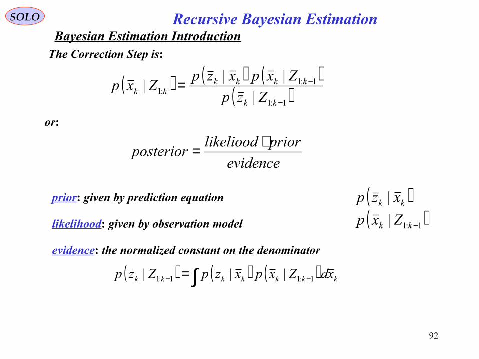
92
Recursive Bayesian EstimationSOLO
The Correction Step is:
( ) ( ) ( )( )1:1
1:1:1 |
|||
−
−=kk
kkkkkk Zzp
ZxpxzpZxp
Bayesian Estimation Introduction
evidence
priorlikelioodposterior
⋅=
or:
prior: given by prediction equation ( )kk xzp |
likelihood: given by observation model ( )1:1| −kk Zxp
evidence: the normalized constant on the denominator
( ) ( ) ( )∫ −− = kkkkkkk xdZxpxzpZzp 1:11:1 |||
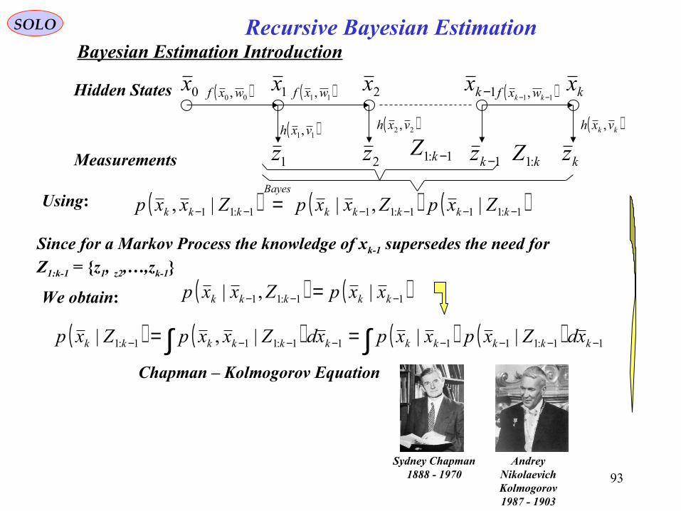
93
Recursive Bayesian EstimationSOLO
( ) ( ) ( )1:111:111:11 |,||, −−−−−− = kkkkk
Bayes
kkk ZxpZxxpZxxp
( ) ( ) ( ) ( )∫∫ −−−−−−−− == 11:11111:111:1 |||,| kkkkkkkkkkk xdZxpxxpxdZxxpZxp
Using:
We obtain:
Since for a Markov Process the knowledge of xk-1 supersedes the need for Z1:k-1 = z1, z2,…,zk-1
( ) ( )11:11 |,| −−− = kkkkk xxpZxxp
Chapman – Kolmogorov Equation
Sydney Chapman1888 - 1970
Andrey Nikolaevich Kolmogorov
1903 - 1987
Bayesian Estimation Introduction
kx1−kx
kz1−kz
0x 1x 2x
1z 2z kZ :11:1 −kZ
( )11, −− kk wxf
( )kk vxh ,
( )00 ,wxf
( )11,vxh
( )11,wxf
( )22 ,vxh
Hidden States
Measurements

94
Recursive Bayesian EstimationSOLO
( ) ( ) ( ) ( )∫∫ −−−−−−−− == 11:11111:111:1 |||,| kkkkkkkkkkk xdZxpxxpxdZxxpZxp
Using p (xk-1|Z1:k-1) from time-step k-1 and p (xk|xk-1) of the Markov system, compute:
Initialize with p (x0)
( ) ( ) ( )( ) ( )∫ −
−=kkkkk
kkkkkk
xdZxpxzp
ZxpxzpZxp
1:1
1:1:1
||
|||
Using p (xk|Z1:k-1) from Prediction phase and p (zk|xk) of the Markov system, compute:
( )∫== kkkkkkkk xdZxpxZxEx :1:1| ||ˆ
( ) ( ) ( ) ( ) ( )∫ −−=−−= kkkT
kkkkkT
kkkkkk xdZxpxxxxZxxxxEP :1:1| |ˆˆ|ˆˆ
At stage k
k:=k+1
( )1|11| ˆˆ −−− = kkkk xfx
0
Prediction phase (before zk measurement)
1
Correction Step (after zk measurement)2
Filtering3
kx1−kx
kz1−kz
0x 1x 2x
1z 2z kZ :11:1 −kZ
( )11, −− kk wxf
( )kk vxh ,
( )00 ,wxf
( )11,vxh
( )11,wxf
( )22 ,vxh
Bayesian Estimation Introduction - Summary
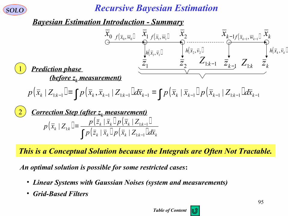
95
Recursive Bayesian EstimationSOLO
( ) ( ) ( ) ( )∫∫ −−−−−−−− == 11:11111:111:1 |||,| kkkkkkkkkkk xdZxpxxpxdZxxpZxp
( ) ( ) ( )( ) ( )∫ −
−=kkkkk
kkkkkk
xdZxpxzp
ZxpxzpZxp
1:1
1:1:1
||
|||
Prediction phase (before zk measurement)
1
Correction Step (after zk measurement)2
kx1−kx
kz1−kz
0x 1x 2x
1z 2z kZ :11:1 −kZ
( )11, −− kk wxf
( )kk vxh ,
( )00 ,wxf
( )11,vxh
( )11,wxf
( )22 ,vxh
Bayesian Estimation Introduction - Summary
This is a Conceptual Solution because the Integrals are Often Not Tractable.
An optimal solution is possible for some restricted cases:
• Linear Systems with Gaussian Noises (system and measurements)
• Grid-Based Filters
Table of Content

96
SOLO
Linear Gaussian Systems
A Linear Combination of Independent Gaussian random vectors is also a Gaussian random vector
mmm XaXaXaS +++= 2211:
( ) ( ) ( )( ) ( )
( ) ( ) ( )
( ) ( )
+++++++−=
+−
+−
+−=
ΦΦ⋅Φ==Φ ∫ ∫+∞
∞−
+∞
∞−
mmmm
mmmm
YYYm
YpYp
mYYmS
aaajaaa
ajaajaaja
YdYdYYpSjm
mmYY
mm
µµµωσσσω
µωσωµωσωµωσω
ωωωωω
2211222
22
22
12
12
22222
22
22
211
21
21
2
11,,
2
1exp
2
1exp
2
1exp
2
1exp
,,exp21
11
1
( ) ( )
−−= 2
2
2exp
2
1,;
i
ii
i
iiiX
XXp
i σµ
σπσµ ( ) ( ) ( )
+−==Φ ∫
+∞
∞−iiiiXiX jXdXpXj
iiµωσωωω 22
2
1expexp:
Moment-Generating
Function
Gaussian distribution
Define
Proof:
( ) ( )iXii
iX
iiYiii Xp
aa
Yp
aYpXaY
iii
11: =
=→=
( ) ( ) ( ) ( ) ( ) ( )
+−=Φ===Φ ∫∫
+∞
∞−
+∞
∞−iiiiiiX
asign
asign
iii
iXiiiiYiY ajaXaXda
a
XpXajYdYpYj
i
i
iiµωσωωωω 222
2
1expexpexp:
1
1
Review of Probability
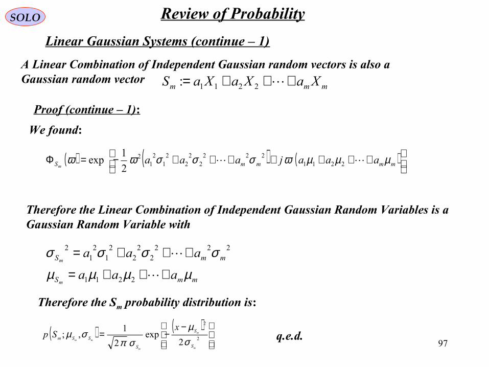
97
SOLO
Linear Gaussian Systems (continue – 1)
A Linear Combination of Independent Gaussian random vectors is also a Gaussian random vector
mmm XaXaXaS +++= 2211:
Therefore the Linear Combination of Independent Gaussian Random Variables is a Gaussian Random Variable with
mmS
mmS
aaa
aaa
m
m
µµµµσσσσ
+++=
+++=
2211
2222
22
21
21
2
Therefore the Sm probability distribution is:
( ) ( )
−−=
2
2
2exp
2
1,;
m
m
m
mm
S
S
S
SSm
xSp
σµ
σπσµ
Proof (continue – 1):
( ) ( ) ( )
+++++++−=Φ mmmmS aaajaaa
mµµµωσσσωω 2211
2222
22
21
21
2
2
1exp
We found:
Review of Probability
q.e.d.

98
Recursive Bayesian EstimationSOLO
Linear Gaussian Markov Systems (continue – 2)
( )( )kkkk
kkkk
vuxkhz
wuxkfx
,,,
,,,1 111
=−= −−−
kkkk
kkkkkkk
vxHz
wuGxx
+=Γ++Φ= −−−−−− 111111
wk-1 and vk, white noises, zero mean, Gaussian, independent
( ) ( ) ( ) ( ) ( ) ( )kPkekeEkxEkxke xTxxx =−= &:
( ) ( ) ( ) ( ) ( ) ( ) lkTwww kQlekeEkwEkwke ,
0
&: δ=−=
( ) ( ) ( ) ( ) ( ) ( ) lkTvvv kRlekeEkvEkvke ,
0
&: δ=−=
( ) ( ) 0=lekeE Tvw
=≠
=lk
lklk 1
0,δ
( ) ( )Qwwpw ,0;N=
( ) ( )Rvvpv ,0;N=
( )( )
−= − wQw
Qwp T
nw1
2/12/ 2
1exp
2
1
π
( )( )
−= − vRv
Rvp T
pv1
2/12/ 2
1exp
2
1
π
A Linear Gaussian Markov Systems is defined as
( ) ( )0|0000 ,;0
Pxxxp ttx == = N ( )( )
( ) ( )
−−−= =
−== 00
10|0002/1
0|02/0 2
1exp
2
10
xxPxxP
xp tT
tntxπ
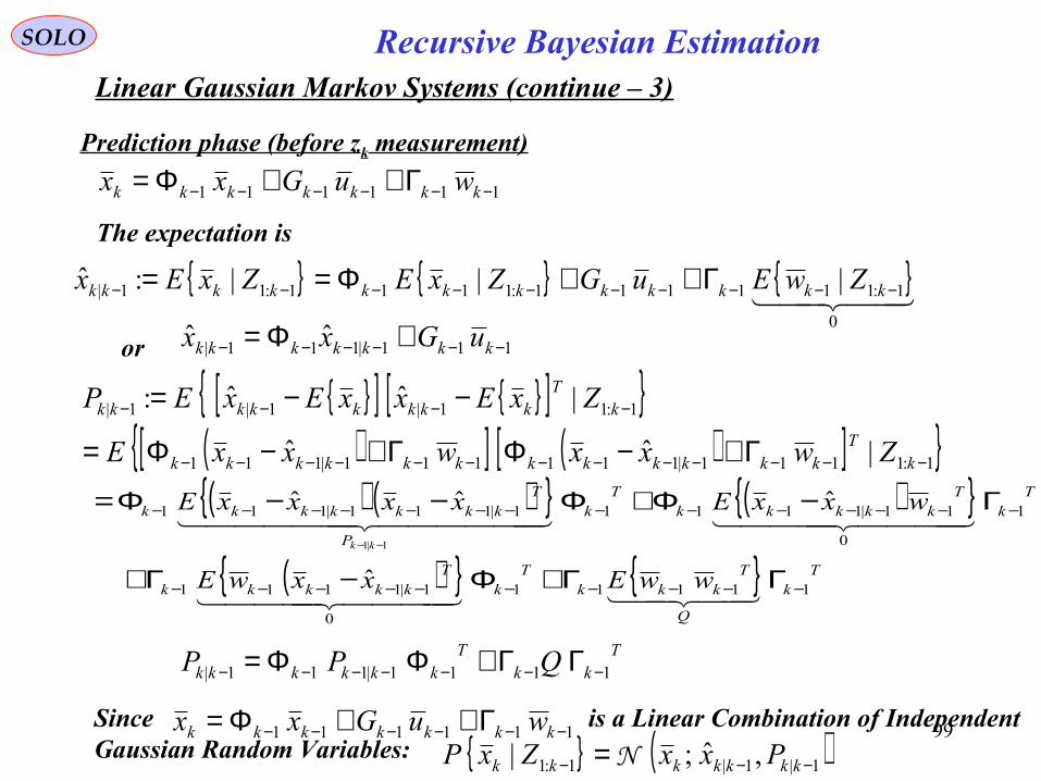
99
Recursive Bayesian EstimationSOLO
Linear Gaussian Markov Systems (continue – 3)
111111 −−−−−− Γ++Φ= kkkkkkk wuGxxPrediction phase (before zk measurement)
0
1:111111:1111:11| |||:ˆ −−−−−−−−−− Γ++Φ== kkkkkkkkkkkk ZwEuGZxEZxEx
or 111|111| ˆˆ −−−−−− +Φ= kkkkkkk uGxx
The expectation is
[ ] [ ] ( )[ ] ( )[ ] 1:1111|111111|111
1:11|1|1|
|ˆˆ
|ˆˆ:
−−−−−−−−−−−−−
−−−−
Γ+−ΦΓ+−Φ=
−−=
kT
kkkkkkkkkkkk
kT
kkkkkkkk
ZwxxwxxE
ZxExxExEP
( ) ( ) ( )
( ) Tk
Q
Tkkk
Tk
Tkkkkk
Tk
Tkkkkk
Tk
P
Tkkkkkkk
wwExxwE
wxxExxxxE
kk
11111
0
1|1111
1
0
11|11111|111|111
ˆ
ˆˆˆ
1|1
−−−−−−−−−−
−−−−−−−−−−−−−−
ΓΓ+Φ−Γ+
Γ−Φ+Φ−−Φ=−−
Tkk
Tkkkkkk QPP 1111|111| −−−−−−− ΓΓ+ΦΦ=
( )1|1|1:1 ,ˆ;| −−− = kkkkkkk PxxZxP NSince is a Linear Combination of Independent Gaussian Random Variables:
111111 −−−−−− Γ++Φ= kkkkkkk wuGxx

100
SOLO
For the particular vector measurement equation
where the measurement noise, is Gaussian (normal), with zero mean: ( ) ( )kkkv Rvvp ,0;N=
( ) ( )( )xp
zxpxzp
x
zxxz
,| ,
| =
and independent of , the conditional probability can be written, using Bayes rule as:
kx ( )xzp xz ||
( )
−
−
==−=
1
111
1111
1
1
,
nxpp
nx
pxnxpxnpxpx
xHz
xHz
zxfxHzv
xn
xn
( ) ( ) 2/1
,, /,, T
vxzx JJvxpzxp =
The measurement noise can be related to and by the function:v zx
pxp
p
pp
p
I
z
f
z
f
z
f
z
f
z
fJ =
∂∂
∂∂
∂∂
∂∂
=
∂∂=
1
1
1
1
( ) ( ) ( ) ( )vpxpvxpzxp vxvxzx ⋅== ,, ,,
kv
Since the measurement noise is independent of :xv
zThe joint probability of and is given by:x
Recursive Bayesian EstimationLinear Gaussian Markov Systems (continue – 4)
kkkk vxHz +=
Correction Step (after zk measurement) - 1st Way
( ) ( ) ( )( )1:1
1:1:1 |
|||
−
−=kk
kkkkkk Zzp
ZxpxzpZxp

101
( ) ( )kkkv Rvvp ,0;N=kkkk vxHz +=
Consider a Gaussian vector , where ,measurement, , where the Gaussian noiseis independent of and .
vkx ( ) [ ]1|1| ,; −−= kkkkkkx Pxxxp
N
kx
( ) ( ) ( ) ( )∫∫+∞
∞−
+∞
∞−
== kkxkkxzkkkzxkz xdxpxzpxdzxpzp |, |,
is Gaussian with( )kz zp ( ) ( ) ( ) ( ) 1|
0
−=+=+= kkkkkkkkk xHvExEHvxHEzE
( ) ( )[ ] ( )[ ] [ ] [ ] ( )[ ] ( )[ ] [ ] [ ] [ ] k
Tkkkk
Tkk
Tk
Tkkkk
Tkkkkk
Tk
Tkkkkkkk
Tkkkkkkkkkk
Tkkkkkkkkkkkk
Tkkkkk
RHPHvvEHxxvEvxxEH
HxxxxEHvxxHvxxHE
xHvxHxHvxHEzEzzEzEz
+=+−−−−
−−=+−+−=
−+−+=−−=
−−−
−−−−
−−
1|
0
1|
0
1|
1|1|1|1|
1|1|cov
( )( ) ( )
( )[ ] ( )[ ] ( )[ ]
−−+−−−−
+−= −
xHzRHPHxHzRHPH
zp TT
Tpz ˆˆ2
1exp
2
1 1
2/12/π
( )( )
( ) ( )
−−−= −
−−−
−
−− 1|1
1|1|2/1
1|2/1:1| 2
1exp
2
1|
1:1 kkkkkT
kkk
kknkkZx xxPxxP
Zxpkk
π
( ) ( )( )
( ) ( )
−−−=−= −
kkkT
kkkpkkkvkkxz xHzRxHzR
xHzpxzp 12/12/| 2
1exp
2
1|
π
Recursive Bayesian EstimationSOLO
Linear Gaussian Markov Systems (continue – 5)Correction Step (after zk measurement) 1st Way (continue – 1)

102
Recursive Bayesian EstimationSOLO
Linear Gaussian Markov Systems (continue – 6)
kkkk vxHz +=
( ) ( )Rvvpv ,0;N=( )
( )
−= − vRv
Rvp T
pv1
2/12/ 2
1exp
2
1
π
Correction Step (after zk measurement) 1st Way (continue – 2)
( )( )
( ) ( )
−−−= −
−−−
−
−− 1|1
1|1|2/1
1|2/1:1| 2
1exp
2
1|
1:1 kkkkkT
kkk
kknkkZx xxPxxP
Zxpkk
π
( ) ( )( )
( ) ( )
−−−=−= −
kkkT
kkkpkkkvkkxz xHzRxHzR
xHzpxzp 12/12/| 2
1exp
2
1|
π
( )( )
[ ] [ ] [ ]
−+−−
+= −
−
−−
−
1|
1
1|1|2/1
1|2/
ˆˆ2
1exp
2
1kkkk
Tkkkk
Tkkk
kTkkkk
pkz xHzRHPHxHz
RHPHzp
π
( ) ( ) ( )( )
( )
( ) ( ) ( ) ( ) [ ] [ ] [ ]
−+−+−−−−−−⋅
+
==
−
−
−−−−
−−−
−
−−
−
1|
1
1|1|1|1
1|1|1
2/1
1|
2/12/1
1|2/1:1
1:1:1
ˆˆ2
1
2
1
2
1exp
2
1
|
|||
kkkkkTkkkk
Tkkkkkkkkk
Tkkkkkkk
Tkkk
kTkkkk
kkknkk
kkkkkk
xHzRHPHxHzxxPxxxHzRxHz
RHPH
RPZzp
ZxpxzpZxp
π
from which
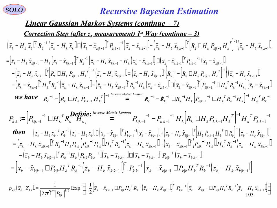
103
( ) ( ) ( ) ( ) ( ) [ ] ( )1|
1
1|1|1|1
1|1|1
−
−
−−−−
−−− −+−−−−+−− kkkk
Tkkkkk
Tkkkkkkkkk
Tkkkkkkk
Tkkk xHzHPHRxHzxxPxxxHzRxHz
( )[ ] ( )[ ] ( ) ( )( ) [ ] ( ) ( ) [ ] ( )( ) ( ) ( ) ( ) ( ) [ ] ( )1|
111|1|1|
11|1|
11|
1|
1
1|1
1|1|
1
1|1|
1|1
1|1|1|1|1
1|1|
−−−
−−−−
−−−
−
−
−
−−
−−
−
−−
−−
−−−−−
−−
−+−+−−−−−−
−+−−=−+−−
−−+−−−−−−=
kkkkkTkkk
Tkkkkkkkk
Tkkkkkkkkk
Tk
Tkkk
kkkkTkkkkkk
Tkkkkkkkk
Tkkkkk
Tkkkk
kkkkkT
kkkkkkkkkkkkT
kkkkkkkk
xxHRHPxxxxHRxHzxHzRHxx
xHzHPHRRxHzxHzHPHRxHz
xxPxxxxHxHzRxxHxHz
[ ] [ ] 11111|
1111
1|1 −−−−
−−−−−
−− ++/−/=+− k
Tkkk
Tkkkkkkk
LemmaMatrixInverseTkkkkkk RHHRHPHRRRHPHRRwe have
Define:[ ] [ ] 11|
1
1|1
1|1
1|
1111|| : −
−
−
−−
−−
−
−−−− +−=+= kk
Tk
Tkkkkkkkkkk
LemmaMatrixInverse
kkTkkkkk PHHPHRHPPHRHPP
( )[ ] ( )[ ]1|1
|1|1
|1|1
|1| −−
−−
−−
− −+−−+−= kkkkkTkkkkkkkk
T
kkkkkTkkkkkk xHzRHPxxPxHzRHPxx
( )( )
( )[ ] ( )[ ]
−+−−+−−⋅= −
−−
−−
−− 1|
1|1|
1|1|
1|1|2/1
|2/:1| 2
1exp
2
1| kkkkk
Tkkkkkkkk
T
kkkkkTkkkkkk
kknkkzx xHzRHPxxPxHzRHPxxP
Zxp
π
Recursive Bayesian EstimationSOLO
Linear Gaussian Markov Systems (continue – 7)Correction Step (after zk measurement) 1st Way (continue – 3)
then ( ) ( ) ( ) ( ) ( ) [ ] ( )1|
1
1|1|1|1
1|1|1
−
−
−−−−
−−− −+−−−−+−− kkkkk
Tkkkk
Tkkkkkkkkk
Tkkkkkkk
Tkkk xHzRHPHxHzxxPxxxHzRxHz
( ) ( ) ( ) ( ) ( ) ( )( ) ( ) ( ) ( ) ( )1|
1|1|1|
1||
11|
1|1
|1
|1|1|1
|1
||1
1|
−−
−−−−
−
−−−
−−−−−
−
−−+−−−
−−−−−=
kkkkkT
kkkkkkkkkkkkT
kkkk
kkkkkTkkkkk
Tkkkkkkkk
Tkkkkkkkkk
Tkkkk
xxPxxxxPPHRxHz
xHzRHPPxxxHzRHPPPHRxHz

104
then
( )kkzxx
Zxpk
:1| |max( )
kk
kkkkkTkkkkkkkk
ZxE
xHzRHPxxx
:1
1|1
|1|*
|
|
ˆˆ:ˆ
=
−+== −−
−
Recursive Bayesian EstimationSOLO
Linear Gaussian Markov Systems (continue – 8)
Correction Step (after zk measurement) 1st Way (continue – 4)
( )( )
( )[ ] ( )[ ]
−+−−+−−⋅= −
−−
−−
−− 1|
11|
1|1|
11|2/1
|2/:1| 2
1exp
2
1| kkkkk
Tkkkkkk
T
kkkkkTkkkk
kknkkzx xHzRHxxPxHzRHxxP
Zxp
π
where:[ ] ( ) ( ) kTkkkkkkkk
Tkkkkk ZxxxxEHRHPP :1||
1111|| ˆˆ: −−=+=
−−−−

105
( ) ( )
ki
kkkkkkkkkkkkkkkkk zzKxxHzKxZxEx 1|1|1|1|:1| ˆ| −−−− −+=−+==
Recursive Bayesian EstimationSOLO
Linear Gaussian Markov Systems (continue – 9)
Summary 1st Way – Kalman Filter
Initial Conditions:
[ ] 1111|| :
−−−− += kk
Tkkkkk HRHPP
Prediction phase (before zk measurement)
111|111| ˆˆ −−−−−− +Φ= kkkkkkk uGxx
Correction Step (after zk measurement)
Tkk
Tkkkkkk QPP 1111|111| −−−−−−− ΓΓ+ΦΦ=
1|: −= k
Tkkkk RHPK
00|0ˆ xEx = ( ) ( ) TxxxxEP 0|000|000|0 ˆˆ: −−=
kkkk wxHz +=
0
1:11|1:11:11| |ˆ||ˆ −−−−− +=+== kkkkkkkkkkkkk ZwExHZwxHEZzEz
1|1| ˆˆ −− = kkkkk xHz

106
Recursive Bayesian EstimationSOLO
Linear Gaussian Markov Systems (continue – 10)
kkkk vxHz +=
( ) ( )Rvvpv ,0;N= ( )( )
−= − vRv
Rvp T
pv1
2/12/ 2
1exp
2
1
π
( )( )
[ ] [ ] [ ]
−+−−
+= −
−
−−
−
1|
1
1|1|2/1
1|2/
ˆˆ2
1exp
2
1kkkkk
Tkkkk
Tkkkk
kT
kkkkp
kz xHzRHPHxHzRHPH
zpπ
from which 1|1:11| ˆ|ˆ −−− == kkkkkkk xHZzEz
( ) ( ) kkT
kkkkkT
kkkkkkzzkk SRHPHZzzzzEP =+=−−= −−−−− :ˆˆ 1|1:11|1|1|
[ ] [ ] [ ] ( )[ ] T
kkkkT
kkkkkkkk
kT
kkkkkkxzkk
HPZvxxHxxE
ZzzxxEP
1|1:11|1|
1:11|1|1|
ˆˆ
ˆˆ
−−−−
−−−−
=+−−=
−−=
We also have
Correction Step (after zk measurement) 2nd Way
Define the innovation: 1|1| ˆˆ: −− −=−= kkkkkk xHzzzi

107
Recursive Bayesian EstimationSOLO
Joint and Conditional Gaussian Random Variables
=
k
kk z
xyDefine: assumed that they are Gaussian distributed
Prediction phase (before zk measurement) 2nd way (continue -1)
=
=
−
−
−
−−
1|
1|
1:1
1:11:1 ˆ
ˆ
|
||
kk
kk
kk
kkkk z
x
Zz
ZxEZyE
=
−
−
−
−=
−−
−−−
−
−
−
−− zz
kkzxkk
xzkk
xxkk
k
T
kkk
kkk
kkk
kkkyykk
PP
PPZ
zz
xx
zz
xxEP
1|1|
1|1|
1:11|
1|
1|
1|
1| ˆ
ˆ
ˆ
ˆ
where: [ ] [ ] 1|1:11|1|1| ˆˆ −−−−− =−−= kkkT
kkkkkkxxkk PZxxxxEP
[ ] [ ] kkT
kkkkkT
kkkkkkzzkk SRHPHZzzzzEP =+=−−= −−−−− :ˆˆ 1|1:11|1|1|
[ ] [ ] Tkkkk
Tkkkkkk
xzkk HPZzzxxEP 1|1:11|1|1| ˆˆ −−−−− =−−=
Linear Gaussian Markov Systems (continue – 11)
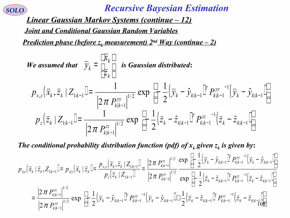
108
( ) ( ) ( )
−−−= −
−−−
−
− 1|
1
1|1|2/1
1|
1:1, ˆˆ2
1exp
2
1|, kkk
yykk
Tkkk
yykk
kkkzx yyPyyP
Zzxpπ
Recursive Bayesian EstimationSOLO
Joint and Conditional Gaussian Random Variables
The conditional probability distribution function (pdf) of xk given zk is given by:
Prediction phase (before zk measurement) 2nd Way (continue – 2)
( ) ( ) ( )
−−−= −
−−−
−
− 1|
1
1|1|2/1
1|
1:1 ˆˆ2
1exp
2
1| kkk
zzkk
Tkkk
zzkk
kkz zzPzzP
Zzpπ
( ) ( ) ( )( )
( ) ( )
( ) ( )
−−−
−−−
===−
−−−
−−
−−
−
−
−
−−
1|
1
1|1|
1|
1
1|1|
2/1
1|
2/1
1|
1:1
1:1,|1:1|
ˆˆ21
exp
ˆˆ21
exp
2
2
|
|,|,|
kkkzzkk
Tkkk
kkkyykk
Tkkk
yykk
zzkk
kkz
kkkzxkkzxkkkzx
zzPzz
yyPyy
P
P
Zzp
ZzxpzxpZzxp
π
π
( ) ( ) ( ) ( )
−−+−−−= −
−−−−
−−−
−
−1|
1
1|1|1|
1
1|1|2/1
1|
2/1
1|ˆˆ
2
1ˆˆ
2
1exp
2
2kkk
zzkk
Tkkkkkk
yykk
Tkkk
yykk
zzkk
zzPzzyyPyyP
P
π
π
Linear Gaussian Markov Systems (continue – 12)
We assumed that is Gaussian distributed:
=
k
kk z
xy
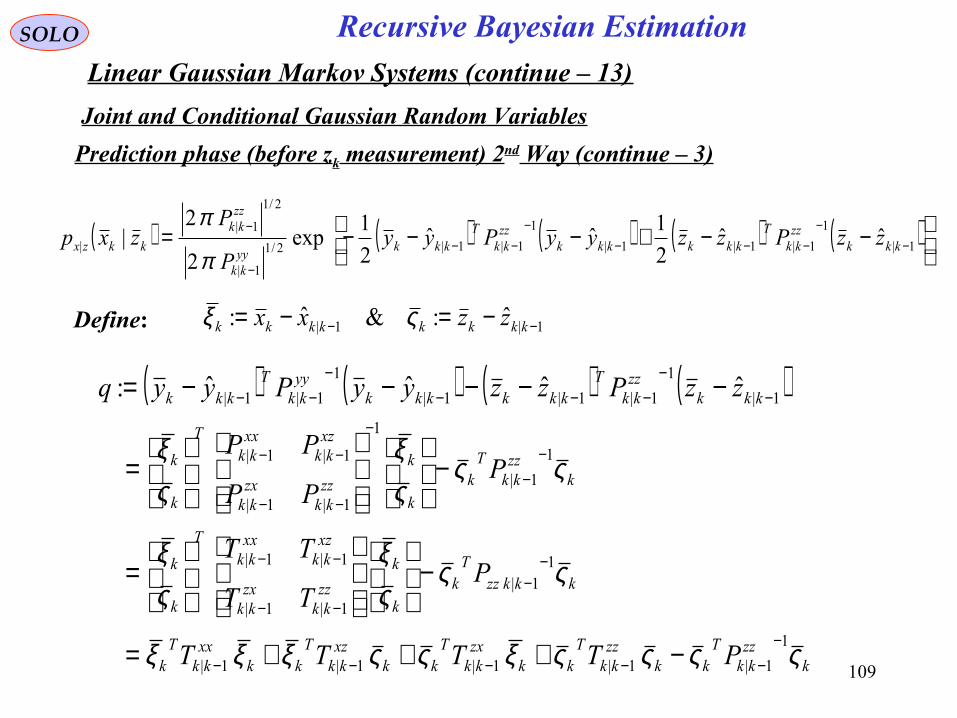
109
Recursive Bayesian EstimationSOLO
Joint and Conditional Gaussian Random Variables
Prediction phase (before zk measurement) 2nd Way (continue – 3)
( ) ( ) ( ) ( ) ( )
−−+−−−= −
−−−−
−−−
−
−1|
1
1|1|1|
1
1|1|2/1
1|
2/1
1|
| ˆˆ2
1ˆˆ
2
1exp
2
2| kkk
zzkk
Tkkkkkk
zzkk
Tkkk
yykk
zzkk
kkzx zzPzzyyPyyP
Pzxp
π
π
Define: 1|1| ˆ:&ˆ: −− −=−= kkkkkkkk zzxx ςξ
( ) ( ) ( ) ( )
kzzkk
Tkk
zzkk
Tkk
zxkk
Tkk
xzkk
Tkk
xxkk
Tk
kkkzzT
k
k
k
zzkk
zxkk
xzkk
xxkk
T
k
k
kzzkk
Tk
k
k
zzkk
zxkk
xzkk
xxkk
T
k
k
kkkzzkk
Tkkkkkk
yykk
Tkkk
PTTTT
PTT
TT
PPP
PP
zzPzzyyPyyq
ςςςςξςςξξξ
ςςςξ
ςξ
ςςςξ
ςξ
1
1|1|1|1|1|
11|
1|1|
1|1|
1
1|
1
1|1|
1|1|
1|
1
1|1|1|
1
1|1| ˆˆˆˆ:
−−−−−−
−−
−−
−−
−−
−
−−
−−
−−
−−−−
−−
−+++=
−
=
−
=
−−−−−=
Linear Gaussian Markov Systems (continue – 13)
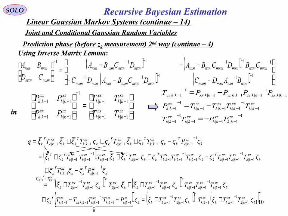
110
Recursive Bayesian EstimationSOLO
Joint and Conditional Gaussian Random Variables
Prediction phase (before zk measurement) 2nd way (continue – 4)Using Inverse Matrix Lemma:
( ) ( )( ) ( )
−−−
−−−=
−−−−−
−−−−−−
11111
111111
nxmnxnmxnmxmmxnmxmnxmnxnmxnmxm
mxmnxmmxnmxmnxmnxnmxnmxmnxmnxn
mxmmxn
nxmnxn
BADCDCBADC
CBDCBADCBA
CD
BA
=
−−
−−
−
−−
−−
zzkk
zxkk
xzkk
xxkk
zzkk
zxkk
xzkk
xxkk
TT
TT
PP
PP
1|1|
1|1|
1
1|1|
1|1|
in1
1|1|1|
1
1|
1|
1
1|1|1|
1
1|
1|1
1|1|1|1
1|
−−−−
−−
−−
−−−−
−
−−
−−−−
−
−=
−=
−=
zzkk
xzkk
xzkk
xxkk
xzkk
xxkk
zxkk
zzkk
zzkk
kkzxkkzzkkxzkkxxkkxx
PPTT
TTTTP
PPPPT
kzzkk
Tkk
zzkk
Tkk
zxkk
Tkk
xzkk
Tkk
xxkk
Tk PTTTTq ςςςςξςςξξξ 1
1|1|1|1|1|
−−−−−− −+++=
( )k
zzkk
Tkk
zzkk
Tk
kxzkk
xxkk
zxkk
Tkk
xzkk
xxkk
zxkk
Tkk
xzkk
Tkk
xxkk
xxkk
zxkk
Tk
Tk
PT
TTTTTTTTTT
ςςςς
ςςςςςξξςξ1
1|1|
1|
1
1|1|1|
1
1|1|1|1|
1
1|1|
−−−
−−
−−−−
−−−−−
−−
−+
−+++=
( ) ( )( ) ( ) ( )k
xzkk
xxkkk
xxkk
T
kxzkk
xxkkkk
zzkk
xzkk
xxkkkkzx
zzkk
Tk
kxzkk
xxkk
xxkk
T
kxzkk
xxkkkk
xxkk
T
kxzkk
xxkkk
TT
TTTTTPTTTT
TTTTTTTTzxkk
Txzkk
ςξςξςς
ςςξξςξ
1|
1
1|1|1|
1
1|
0
1|1|
1
1|1|1|
1|
1
1|1|1|
1
1|1|1|
1
1|
1|1|
−−
−−−−
−−−−
−−−
−−
−−−−
−−−−
−
=
++=−−+
+++=−−
Linear Gaussian Markov Systems (continue – 14)

111
Recursive Bayesian EstimationSOLO
Joint and Conditional Gaussian Random Variables
Prediction phase (before zk measurement) 2nd way (continue – 5)
=
−−
−−
−
−−
−−
zzkk
zxkk
xzkk
xxkk
zzkk
zxkk
xzkk
xxkk
TT
TT
PP
PP
1|1|
1|1|
1
1|1|
1|1|
1
1|1|1|
1
1|
1|
1
1|1|1|
1
1|
1|1
1|1|1|1
1|
−−−−
−−
−−
−−−−
−
−−
−−−−
−
−=
−=
−=
zzkk
xzkk
xzkk
xxkk
xzkk
xxkk
zxkk
zzkk
zzkk
kkzxkkzzkkxzkkxxkkxx
PPTT
TTTTP
PPPPT
( ) ( )kxzkk
xxkkk
xxkk
T
kxzkk
xxkkk TTTTTq ςξςξ 1|
1
1|1|1|
1
1| −−
−−−−
− ++=
1|1| ˆ:&ˆ: −− −=−= kkkkkkkk zzxx ςξ
( )
( )[ ] ( )[ ]
−−−−−−−=
−=
−−−−−
−
−
−
−
1|1|1|1|1|2/1
1|
2/1
1|
2/1
1|
2/1
1|
|
ˆˆˆˆ2
1exp
2
2
2
1exp
2
2|
kkkkkkkxxkk
Tkkkkkkk
yykk
zzkk
yykk
zzkk
kkzx
zzKxxTzzKxxP
P
qP
Pzxp
π
π
π
π
( )1|
1
1|1|1|
1
1|1| ˆˆ −−
−−−−
−− −−−=+ kkk
K
zzkk
xzkkkkkk
xxkk
xzkkk zzPPxxTT
k
ςξ
Linear Gaussian Markov Systems (continue – 15)

112
Recursive Bayesian EstimationSOLO
Joint and Conditional Gaussian Random Variables
Prediction phase (before zk measurement) 2nd Way (continue – 6)
( ) ( )[ ] ( )[ ]
−−−−−−−= −
−−−−−−
−−−− 1|
1
1|1|1|1|1|
1
1|1|1|| ˆˆˆˆ2
1exp| kkk
xxkk
xzkkkkk
xxkk
T
kkkxxkk
xzkkkkkkkzx zzPPxxTzzPPxxczxp
From this we can see that
( )1|
1
1|1|1|| ˆˆˆ| −−
−−− −+== kkk
K
zzkk
xzkkkkkkkk zzPPxxzxE
k
( ) ( ) T
kzzkkk
xxkk
zxkk
zzkk
xzkk
xxkk
xxkkk
Tkkkkkk
xxkk
KPKP
PPPPTZxxxxEP
1|1|
1|
1
1|1|1|
1
1|:1||| ˆˆ
−−
−−
−−−−
−
−=
−==−−=
[ ] [ ] 1|1:11|1|1| ˆˆ −−−−− =−−= kkkT
kkkkkkxxkk PZxxxxEP
[ ] [ ] kT
kkkkkkT
kkkkkkzzkk SHPHRZzzzzEP =+=−−= −−−−− :ˆˆ 1|1:11|1|1|
[ ] [ ] Tkkkk
Tkkkkkk
xzkk HPZzzxxEP 1|1:11|1|1| ˆˆ −−−−− =−−=
Linear Gaussian Markov Systems (continue – 16)
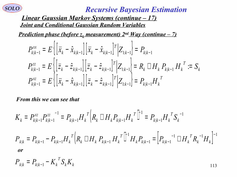
113
Recursive Bayesian EstimationSOLO
Joint and Conditional Gaussian Random Variables
Prediction phase (before zk measurement) 2nd Way (continue – 7)
From this we can see that
( ) [ ] 1111|1|
1
1|1|1||
−−−−−
−
−−− +=+−= kkT
kkkkkkT
kkkkkT
kkkkkkk HRHPPHHPHRHPPP
( ) 11|
1
1|1|
1
1|1|−
−
−
−−−
−− =+== kT
kkkT
kkkkkT
kkkzzkk
xzkkk SHPHPHRHPPPK
Linear Gaussian Markov Systems (continue – 17)
kkT
kkkkk KSKPP −= −1||
or
[ ] [ ] 1|1:11|1|1| ˆˆ −−−−− =−−= kkkT
kkkkkkxxkk PZxxxxEP
[ ] [ ] kT
kkkkkkT
kkkkkkzzkk SHPHRZzzzzEP =+=−−= −−−−− :ˆˆ 1|1:11|1|1|
[ ] [ ] Tkkkk
Tkkkkkk
xzkk HPZzzxxEP 1|1:11|1|1| ˆˆ −−−−− =−−=
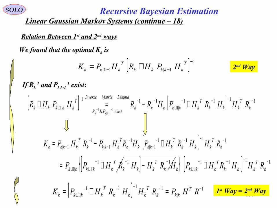
114
We found that the optimal Kk is
[ ] 11|1|
−
−− += Tkkkkk
Tkkkk HPHRHPK
[ ] [ ] 1111|1
11
&
1
|1 11|
1
−−−−+
−−−
+ +−=+−
−− k
Tkkk
Tkkkkkk
LemmaMatrixInverse
existPR
Tkkkkk RHHRHPHRRHPHR
kkk
[ ] 11111|
11|
11|
−−−−−
−−
−− +−= k
Tkkk
Tkkkkk
Tkkkk
Tkkkk RHHRHPHRHPRHPK
[ ] [ ] 1111|1
111|1|1
−−−−+
−−−++ +−+= k
Tkkk
Tkkkkk
Tkkk
Tkkkkk RHHRHPHRHHRHPP
[ ] 1|
1111|1
−−−−−+ =+= RHPRHHRHPK T
kkkT
kkkT
kkkk
If Rk-1 and Pk|k-1
-1 exist:
Recursive Bayesian EstimationSOLO
Linear Gaussian Markov Systems (continue – 18)
Relation Between 1st and 2nd ways
2nd Way
1st Way = 2nd Way

115
1|1| ˆˆ: −− −=−= kkkkkkkk zzxHzi
Recursive Bayesian EstimationSOLO
Linear Gaussian Markov Systems (continue – 19)Innovation
The innovation is the quantity:
We found that:
( ) 0ˆ||ˆ| 1|1:11:11|1:1 =−=−= −−−−− kkkkkkkkkk zZzEZzzEZiE
[ ] [ ] kT
kkkkkkT
kkkT
kkkkkk SHPHRZiiEZzzzzE =+==−− −−−−− :ˆˆ 1|1:11:11|1|
Using the smoothing property of the expectation:
( ) ( ) ( ) ( )( )
( ) ( ) xEdxxpxdxdyyxpx
dxdyypyxpxdyypdxyxpxyxEE
x
X
x y
YX
x yyxp
YYX
y
Y
x
YX
YX
==
=
=
=
∫∫ ∫
∫ ∫∫ ∫
∞+
−∞=
∞+
−∞=
∞+
−∞=
∞+
−∞=
∞+
−∞=
∞+
−∞=
∞+
−∞=
,
||
,
,
||
,
1:1 −= kT
jkT
jk ZiiEEiiEwe have:
Assuming, without loss of generality, that k-1 ≥ j, and innovation I (j) is Independent on Z1:k-1, and it can be taken outside the inner expectation:
0
0
1:11:1 =
== −−T
jkkkT
jkT
jk iZiEEZiiEEiiE

116
1|1| ˆˆ: −− −=−= kkkkkkkk zzxHzi
Recursive Bayesian EstimationSOLO
Linear Gaussian Markov Systems (continue – 20)Innovation (continue – 1)
The innovation is the quantity:
We found that:
( ) 0ˆ||ˆ| 1|1:11:11|1:1 =−=−= −−−−− kkkkkkkkkk zZzEZzzEZiE
kT
kkkkkkT
kk SHPHRZiiE =+= −− :1|1:1
0=Tjk iiE
jikT
jk SiiE δ=
The uncorrelated ness property of the innovation implies that since they are Gaussian,the innovation are independent of each other and thus the innovation sequence isStrictly White.
Thus the innovation sequence is zero mean and white for the Kalman (Optimal) Filter.
Without the Gaussian assumption, the innovation sequence is Wide Sense White.
Table of Content

117
Recursive Bayesian EstimationSOLO
Closed-Form Solutions of Estimation
Closed-Form solutions for the Optimal Recursive Bayesian Estimationcan be derived only for special cases
The most important case:
• Dynamic and measurement models are linear
( )( )kkkk
kkkk
vuxkhz
wuxkfx
,,,
,,,1 111
=−= −−−
kkkk
kkkkkkk
vxHz
wuGxx
+=Γ++Φ= −−−−−− 111111
• Random noises are Gaussian
( ) ( )Qwwpw ,0;N=
( ) ( )Rvvpv ,0;N=
( )( )
−= wQw
Qwp T
nw 2
1exp
2
12/12/π
( )( )
−= − vRv
Rvp T
pv1
2/12/ 2
1exp
2
1
π• Solution: KALMAN FILTER
• In other non-linear/non-Gaussian cases:
USE APPROXIMATIONS

118
Recursive Bayesian EstimationSOLO
Closed-Form Solutions of Estimation (continue – 1)
• Dynamic and measurement models are linear
kkkk
kkkkkkk
vxHz
wuGxx
+=Γ++Φ= −−−−−− 111111
• The Optimal Estimator is the Kalman Filter developed by R. E. Kalman in 1960
( ) ( ) ( ) ( ) ( ) ( )kPkekeEkxEkxke xT
xxx =−= &:
( ) ( ) ( ) ( ) ( ) ( ) lkT
www kQlekeEkwEkwke ,
0
&: δ=−=
( ) ( ) ( ) ( ) ( ) ( ) lkT
vvv kRlekeEkvEkvke ,
0
&: δ=−= ( ) ( ) 0=lekeE T
vw
=≠
=lk
lklk 1
0,δ
Rudolf E. Kalman( 1920 - )
• K.F. is an Optimal Estimator (in the Minimum Mean Square Estimator (MMSE) ) sense if: - state and measurement models are linear - the random elements are Gaussian
• Under those conditions, the covariance matri: - independent of the state (can be calculated off-line) - equals the Cramer – Rao lower bound
Table of Content

119
Kalman FilterState Estimation in a Linear System (one cycle)
SOLO
1: += kk
Initialization ( ) ( ) TxxxxEPxEx 00000|000 ˆˆˆ −−==0
State vector prediction111|111| ˆˆ −−−−−− +Φ= kkkkkkk uGxx1
Covariance matrix extrapolation111|111| −−−−−− +ΦΦ= kT
kkkkkk QPP2
Innovation CovariancekT
kkkkk RHPHS += −1|3
Gain Matrix Computation11|
−−= k
Tkkkk SHPK4
Measurement & Innovation1|ˆ
1|ˆ
−
−−=kkz
kkkkk xHzi5
Filteringkkkkkk iKxx += −1|| ˆˆ6
Covariance matrix updating
( )( ) ( ) T
kkkT
kkkkkk
kkkk
Tkkkkk
kkkkT
kkkkkkk
KRKHKIPHKI
PHKI
KSKP
PHSHPPP
+−−=
−=−=
−=
−
−
−
−−
−−
1|
1|
1|
1|1
1|1||7

120
Kalman FilterState Estimation in a Linear System (one cycle)
Sensor DataProcessing andMeasurement
Formation
Observation -to - Track
Association
InputData Track Maintenance
( Initialization,Confirmationand Deletion)
Filtering andPrediction
GatingComputations
Samuel S. Blackman, " Multiple-Target Tracking with Radar Applications", Artech House,1986
Samuel S. Blackman, Robert Popoli, " Design and Analysis of Modern Tracking Systems",Artech House, 1999
SOLO
Rudolf E. Kalman( 1920 - )

121
SOLO
General Bayesian Nonlinear Filters
General Bayesian Nonlinear Filters
Additive GaussianNoise
Gauss Hermite Kalman Filter
(GHKF)
Unscented Kalman Filter
(UKF)
Non-ResamplingParticleFilter
Gaussian Particle
Filter (GPF)
Gauss Hermite Particle Filter
(GHPF)
Unscented Particle Filter
(UPF)
Monte CarloParticle Filter
(MCPF)
Recursive Bayesian Estimation
Monte CarloKalman Filter
(MCKF)
ExtendedKalman Filter
(EKF)
Non-AdditiveNon-Gaussian
Noise
ResamplingParticleFilter
Sequential Importance Sampling Particle
Filter (SIS PF)
Bootstrap Particle
Filter (BPF)
Run This
Table of Content

122
Extended Kalman FilterSensor Data
Processing andMeasurement
Formation
Observation -to - Track
Association
InputData Track Maintenance
( Initialization,Confirmationand Deletion)
Filtering andPrediction
GatingComputations
Samuel S. Blackman, " Multiple-Target Tracking with Radar Applications", Artech House,1986
Samuel S. Blackman, Robert Popoli, " Design and Analysis of Modern Tracking Systems",Artech House, 1999
SOLO
In the extended Kalman filter, (EKF) the state transition and observation models need not be linear functions of the state but may instead be (differentiable) functions.
( ) ( ) ( )[ ] ( )kwkukxkfkx +=+ ,,1
( ) ( ) ( )[ ] ( )11,1,11 +++++=+ kkukxkhkz νState vector dynamics
Measurements
( ) ( ) ( ) ( ) ( ) ( )kPkekeEkxEkxke xT
xxx =−= &:
( ) ( ) ( ) ( ) ( ) ( ) lkT
www kQlekeEkwEkwke ,
0
&: δ=−=
( ) ( ) lklekeE Tvw ,0 ∀=
=≠
=lk
lklk 1
0,δ
The function f can be used to compute the predicted state from the previous estimate and similarly the function h can be used to compute the predicted measurement from the predicted state. However, f and h cannot be applied to the covariance directly. Instead a matrix of partial derivatives (the Jacobian) is computed.
( ) ( ) ( )[ ] ( ) ( )[ ] ( )( )
( ) ( )( )
( ) ( )kekex
fkeke
x
fkekukxEkfkukxkfke wx
Hessian
kxE
Txx
Jacobian
kxE
wx ++∂∂+
∂∂=+−=+
2
2
2
1,,,,1
( ) ( ) ( )[ ] ( ) ( )[ ] ( )( )
( ) ( )( )
( ) ( )1112
1111,1,11,1,11
1
2
2
1
++++∂∂+++
∂∂=+++++−+++=+
++
kkex
hkeke
x
hkkukxEkhkukxkhke x
Hessian
kxE
Txx
Jacobian
kxE
z νν
Taylor’s Expansion:

123
Extended Kalman FilterState Estimation (one cycle)
SOLO
1: += kk
( )11|11| ,ˆ,1ˆ −−−− −= kkkkk uxkfxState vector prediction1
Jacobians Computation
1|1|1 ˆˆ
1 &−−−
∂∂=
∂∂=Φ −
kkkk x
k
x
k x
hH
x
f2
Covariance matrix extrapolation111|111| −−−−−− +ΦΦ= kT
kkkkkk QPP3
Innovation CovariancekT
kkkkk RHPHS += −1|4
Gain Matrix Computation11|
−−= k
Tkkkk SHPK5
Measurement & Innovation1|ˆ
1|ˆ
−
−−=kkz
kkkkk xHzi6
Filteringkkkkkk iKxx += −1|| ˆˆ7
Covariance matrix updating
( )( ) ( ) T
kkkT
kkkkkk
kkkk
Tkkkkk
kkkkT
kkkkkkk
KRKHKIPHKI
PHKI
KSKP
PHSHPPP
+−−=
−=−=
−=
−
−
−
−−
−−
1|
1|
1|
1|1
1|1||8
0 Initialization (k = 0) ( ) ( ) TxxxxEPxEx 00000|000 ˆˆˆ −−==

124
Extended Kalman FilterState Estimation (one cycle)
Sensor DataProcessing andMeasurement
Formation
Observation -to - Track
Association
InputData Track Maintenance
( Initialization,Confirmationand Deletion)
Filtering andPrediction
GatingComputations
Samuel S. Blackman, " Multiple-Target Tracking with Radar Applications", Artech House,1986
Samuel S. Blackman, Robert Popoli, " Design and Analysis of Modern Tracking Systems",Artech House, 1999
SOLO
Rudolf E. Kalman( 1920 - )

125
SOLO
Criticism of the Extended Kalman FilterUnlike its linear counterpart, the extended Kalman filter is not an optimal estimator. In addition, if the initial estimate of the state is wrong, or if the process is modeled incorrectly, the filter may quickly diverge, owing to its linearization. Another problem with the extended Kalman filter is that the estimated covariance matrix tends to underestimate the true covariance matrix and therefore risks becoming inconsistent in the statistical sense without the addition of "stabilizing noise".Having stated this, the Extended Kalman filter can give reasonable performance, and is arguably the de facto standard in navigation systems and GPS.
Extended Kalman Filter
Table of Content
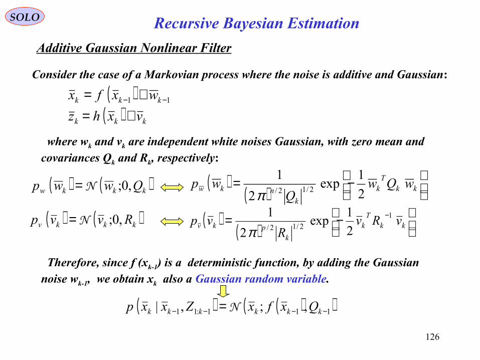
126
SOLO
Additive Gaussian Nonlinear Filter
Consider the case of a Markovian process where the noise is additive and Gaussian:
( )( ) kkk
kkk
vxhz
wxfx
+=+= −− 11
( ) ( )kkkw Qwwp ,0;N=
( ) ( )kkkv Rvvp ,0;N=
( )( )
−= kk
Tk
knkw wQw
Qwp
2
1exp
2
12/12/π
( )( )
−= −
kkT
k
kpkv vRv
Rvp 1
2/12/ 2
1exp
2
1
π
where wk and vk are independent white noises Gaussian, with zero mean and covariances Qk and Rk, respectively:
Recursive Bayesian Estimation
Therefore, since f (xk-1) is a deterministic function, by adding the Gaussian noise wk-1, we obtain xk also a Gaussian random variable.
( ) ( )( )111:11 ,;,| −−−− = kkkkkk QxfxZxxp N

127
SOLO
Additive Gaussian Nonlinear Filter (continue – 1) ( )( ) kkk
kkk
vxhz
wxfx
+=+= −− 11
Recursive Bayesian Estimation
( ) ( )( )111:11 ,;,| −−−− = kkkkkk QxfxZxxp N
( ) ( ) ( )1:111:111:11 |,||, −−−−−− = kkkkk
Bayes
kkk ZxpZxxpZxxp
( ) ( ) ( ) ( )∫∫ −−−−−−−−− == 11:111:1111:111:1 |,||,| kkkkkkkkkkkk xdZxpZxxpxdZxxpZxp
Using:
we obtain:
( ) ( )( ) ( )∫ −−−−−− = 11:11111:1 |,;| kkkkkkkk xdZxpQxfxZxp N
( ) ( )( ) ( )[ ]∫ ∫∫ −−−−−−−− === kkkkkkkkkkkkkkkk xdxdZxpQxfxxxdZxpxZxEx 11:11111:11:11| |,;||:ˆ N
( )( )[ ] ( ) ( ) ( )∫∫ ∫ −−−−−−−−− == 11:11111:1111 ||,; kkkkkkkkkkkk xdZxpxfxdZxpxdQxfxx N
Assume that is Gaussian with mean and covariance , then1−kx1|1ˆ −− kkx 1|1 −− kkP
( ) ( )1|11|111:11 ,ˆ;| −−−−−−− = kkkkkkk PxxZxp N
( ) ( )∫ −−−−−−−−− == 11|11|1111:11| ,ˆ;|ˆ kxx
kkkkkkkkkk xdPxxxfZxEx N
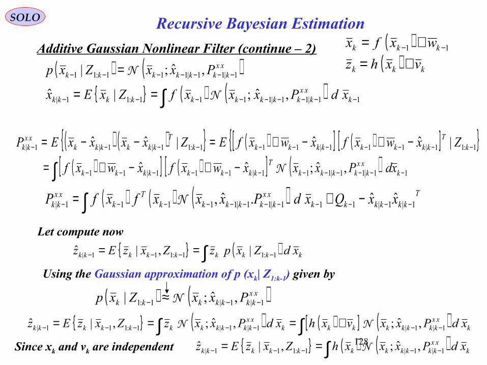
128
SOLO
Additive Gaussian Nonlinear Filter (continue – 2) ( )( ) kkk
kkk
vxhz
wxfx
+=+= −− 11
Recursive Bayesian Estimation
( ) ( )xxkkkkkkk PxxZxp 1|11|111:11 ,ˆ;| −−−−−−− = N
( ) ( )∫ −−−−−−−−− == 11|11|1111:11| ,ˆ;|ˆ kxx
kkkkkkkkkk xdPxxxfZxEx N
( ) ( ) ( )[ ] ( )[ ] ( )[ ] ( )[ ] ( )∫ −−−−−−−−−−−−
−−−−−−−−−−−
−+−+=
−+−+=−−=
11|11|111|111|11
1:11|111|111:11|1|1|
,ˆ;ˆˆ
|ˆˆ|ˆˆ
kxx
kkkkkT
kkkkkkkk
kT
kkkkkkkkkT
kkkkkkxx
kk
xdPxxxwxfxwxf
ZxwxfxwxfEZxxxxEP
N
( ) ( ) ( ) Tkkkkkk
xxkkkkkk
Tk
xxkk xxQxdPxxxfxfP 1|1|111|11|11111| ˆˆ.ˆ, −−−−−−−−−−−− −+= ∫ N
Let compute now
( )∫ −−−− == kkkkkkkkk xdZxpzZxzEz 1:11:111| |,|ˆ
( ) ( )[ ] ( )∫∫ −−−−−−− +=== kxx
kkkkkkkkxx
kkkkkkkkkkk xdPxxvxhxdPxxzZxzEz 1|1|1|1|1:111| ,ˆ;,ˆ;,|ˆ NN
Since xk and vk are independent ( ) ( )∫ −−−−− == kxx
kkkkkkkkkkk xdPxxxhZxzEz 1|1|1:111| ,ˆ;,|ˆ N
Using the Gaussian approximation of p (xk| Z1:k-1) given by
( ) ( )xxkkkkkkk PxxZxp 1|1|1:1 ,ˆ;| −−− ≈N

129
SOLO
Additive Gaussian Nonlinear Filter (continue – 3) ( )( ) kkk
kkk
vxhz
wxfx
+=+= −− 11
Recursive Bayesian Estimation
( ) ( )xxkkkkkkk PxxZxp 1|1|1:1 ,ˆ;| −−− ≈N
Since xk and vk are independent
( ) ( )∫ −−−−− == kxx
kkkkkkkkkkk xdPxxxhZxzEz 1|1|1:111| ,ˆ;,|ˆ N
( ) ( ) ( )[ ] ( )[ ] ( )[ ] ( )[ ] ( )∫ −−−−
−−−−−−−
−+−+=
−+−+=−−=
kxx
kkkkkT
kkkkkkkk
kT
kkkkkkkkkT
kkkkkkzzkk
xdPxxzvxhzvxh
ZzvxhzvxhEZzzzzEP
1|1|1|1|
1:11|1|1:11|1|1|
.ˆ,ˆˆ
|ˆˆ|ˆˆ
N
( ) ( ) ( ) Tkkkkkk
xxkkkkkk
Tk
zzkk zzRxdPxxxhxhP 1|1|1|1|1| ˆˆ,ˆ; −−−−− −+= ∫ N
In the same way
( ) ( ) ( ) ( )[ ] ( ) ( )[ ] ( )∫ −−−−
−−−−−−−
−+−=
−+−=−−=
kxx
kkkkkT
kkkkkkk
kT
kkkkkkkkT
kkkkkkzx
kk
xdPxxzvxhxx
ZzvxhxxEZzzxxEP
1|1|1|1|
1:11|1|1:11|1|1|
.ˆ,ˆˆ
|ˆˆ|ˆˆ
N
( ) ( ) Tkkkkk
xxkkkkkk
Tk
zxkk zxxdPxxxhxP 1|1|1|1|1| ˆˆ,ˆ; −−−−− −= ∫ N

130
SOLO
Additive Gaussian Nonlinear Filter (continue – 4) ( )( ) kkk
kkk
vxhz
wxfx
+=+= −− 11
Recursive Bayesian Estimation
( ) ( )∫ −−−−− == kxx
kkkkkkkkkkk xdPxxxhZxzEz 1|1|1:111| ,ˆ;,|ˆ N
( ) ( ) ( ) Tkkkkkk
xxkkkkkk
Tk
zzkk zzRxdPxxxhxhP 1|1|1|1|1| ˆˆ,ˆ; −−−−− −+= ∫ N
( ) ( ) Tkkkkk
xxkkkkkk
Tk
zxkk zxxdPxxxhxP 1|1|1|1|1| ˆˆ,ˆ; −−−−− −= ∫ N
( ) ( )∫ −−−−−−−−− == 11|11|1111:11| .ˆ;|ˆ kxx
kkkkkkkkkk xdPxxxfZxEx N
( ) ( ) ( ) Tkkkkkk
xxkkkkkk
Tk
xxkk xxQxdPxxxfxfP 1|1|111|11|11111| ˆˆ,ˆ; −−−−−−−−−−−− −+= ∫ N
Summary
Initialization0
( ) ( ) TxxxxEP
xEx
00000|0
00
ˆˆ
ˆ
−−=
=
For ∞∈ ,,1k
State Prediction and its Covariance1
Measure Prediction and Covariances2
kx1−kx
kz1−kz
0x 1x 2x
1z 2z kZ :11:1 −kZ
( ) 11 −− + kk wxf
( ) kk vxh +
( ) 00 wxf +
( ) 11 vxh +
( ) 11 wxf +
( ) 22 vxh +
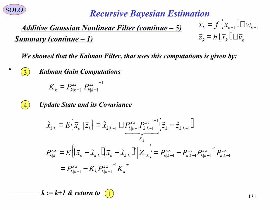
131
SOLO
Additive Gaussian Nonlinear Filter (continue – 5) ( )( ) kkk
kkk
vxhz
wxfx
+=+= −− 11
Recursive Bayesian Estimation
Summary (continue – 1)
We showed that the Kalman Filter, that uses this computations is given by:
( )1|
1
1|1|1|| ˆˆ|ˆ −−
−−− −+== kkk
K
zzkk
zxkkkkkkkk zzPPxzxEx
k
( ) ( ) T
kzzkkk
xxkk
xzkk
zzkk
zxkk
xxkkk
Tkkkkkk
xxkk
KPKP
PPPPZxxxxEP
1
1|1|
1|
1
1|1|1|:1||| ˆˆ
−−−
−−
−−−
−=
−=−−=
Kalman Gain Computations31
1|1|
−−−= zz
kkxzkkk PPK
k := k+1 & return to 1
Update State and its Covariance4
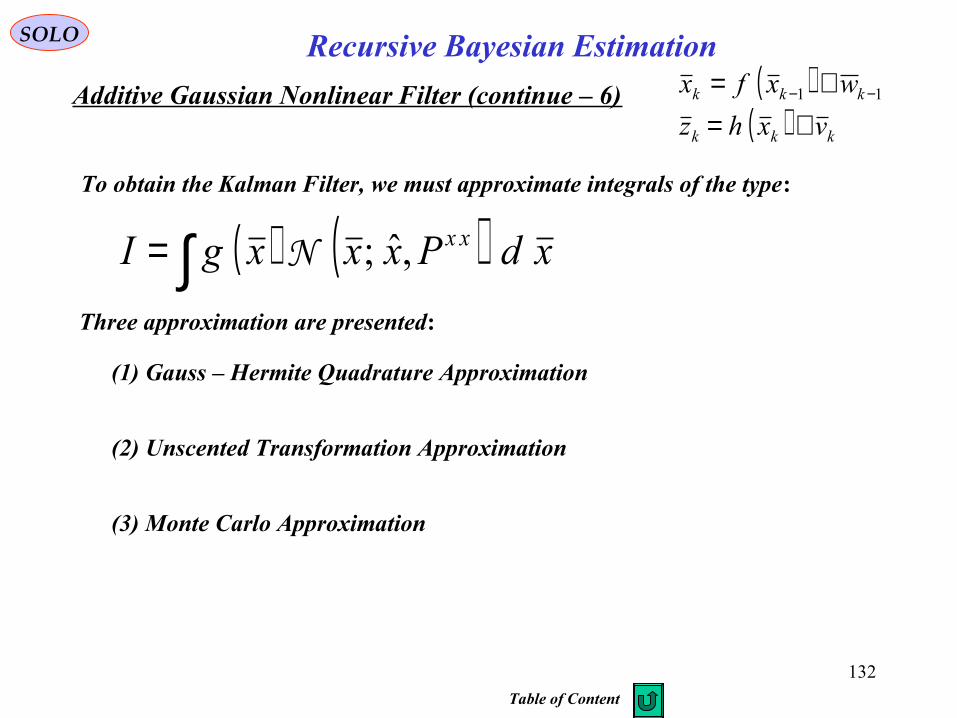
132
SOLO
Additive Gaussian Nonlinear Filter (continue – 6) ( )( ) kkk
kkk
vxhz
wxfx
+=+= −− 11
Recursive Bayesian Estimation
( ) ( )∫= xdPxxxgI xx,ˆ;N
To obtain the Kalman Filter, we must approximate integrals of the type:
Three approximation are presented:
(1) Gauss – Hermite Quadrature Approximation
(2) Unscented Transformation Approximation
(3) Monte Carlo Approximation
Table of Content

133
SOLO
Additive Gaussian Nonlinear Filter (continue – 7)( )
( ) kkk
kkk
vxhz
wxfx
+=+= −− 11
Recursive Bayesian Estimation
( ) ( )∫= xdPxxxgI xx,ˆ;N
To obtain the Kalman Filter, we must approximate integrals of the type:
Gauss – Hermite Quadrature Approximation
( )( )[ ] ( ) ( )∫
−−−= − xdxxPxx
PxgI xx
T
xxn
ˆˆ2
1exp
2
1 1
2/1π
Let Pxx = STS a Cholesky decomposition, and define: ( )xxSz ˆ2
1: 1 −= −
( ) ( )∫ −= zdezgI zzn
T
2/2
2
π
This integral can be approximated using the Gauss – Hermite quadrature rule:
( ) ( )∑∫=
− ≈M
iii
z zfwzdzfe1
2
where the quadrature points zi and weights wi are defined as follows:
Carl Friedrich Gauss
1777 - 1855
Charles Hermite1822 - 1901
Andre – LouisCholesky1875 - 1918

134
SOLO
Additive Gaussian Nonlinear Filter (continue – 8)( )
( ) kkk
kkk
vxhz
wxfx
+=+= −− 11
Recursive Bayesian Estimation
Gauss – Hermite Quadrature Approximation (continue – 1)
( ) ( )∑∫=
− ≈M
iii
z zfwzdzfe1
2
The quadrature points zi and weights wi are defined as follows:
A set of orthonormal Hermite polynomials are generated from the recurrence relationship:( ) ( )
( ) ( ) ( )zHj
jzH
jzzH
zHzH
jjj 11
4/101
11
2
/1,0
−+
−
+−
+=
== π
or in matrix form:
( )( )
( )( )
( )( )
( )( )
( ) Mjj
zH
zH
zH
zH
zH
zH
zH
z jM
e
M
zh
M
J
M
M
zh
M
M
M
,,2,12
:
1
0
0
0
00
00
00
00
00
1
1
0
1
1
2
21
1
1
1
0
==
+
=
−
−
−−
ββ
ββ
βββ
β
( )
( ) ( )zHj
zHj
zHz jjj
jj
11
1
2
1
2 +−
+
++=
ββ
( ) ( ) ( )zHezhJzhz MMMM β+=
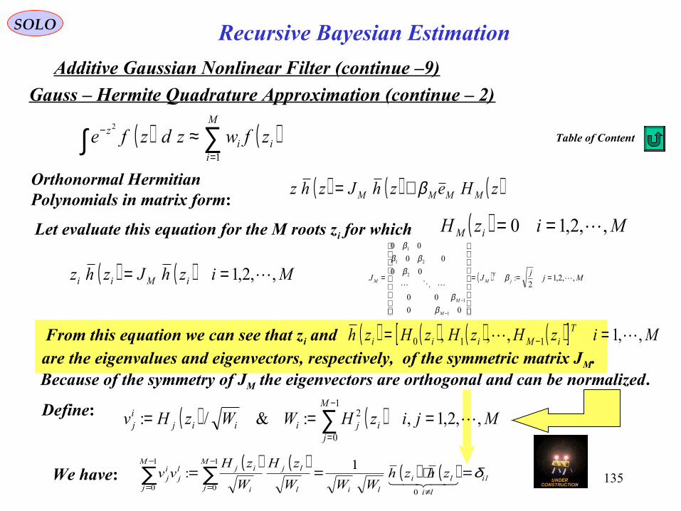
135
SOLO
Additive Gaussian Nonlinear Filter (continue –9)
Recursive Bayesian Estimation
Gauss – Hermite Quadrature Approximation (continue – 2)
( ) ( )∑∫=
− ≈M
iii
z zfwzdzfe1
2
Orthonormal HermitianPolynomials in matrix form:
( ) Mjj
JJ jT
M
M
M
M ,,2,12
:
00
00
00
00
00
1
1
2
21
1
===
=
−
−
β
ββ
βββ
β
( ) ( ) ( )zHezhJzhz MMMM β+=
Let evaluate this equation for the M roots zi for which ( ) MizH iM ,,2,10 ==
( ) ( ) MizhJzhz iMii ,,2,1 ==
From this equation we can see that zi andare the eigenvalues and eigenvectors, respectively, of the symmetric matrix JM.
( ) ( ) ( ) ( )[ ] MizHzHzHzh TiMiii ,,1,,, 110 == −
Because of the symmetry of JM the eigenvectors are orthogonal and can be normalized.
Define: ( ) ( ) MjizHWWzHvM
jijiiij
ij ,,2,1,:&/:
1
0
2 === ∑−
=
We have:( ) ( ) ( ) ( ) li
li
li
li
M
j l
lj
i
ijM
j
lj
ij zhzh
WWW
zH
W
zHvv δ=⋅==
≠
−
=
−
=∑∑
0
1
0
1
0
1:
Table of Content

136
Unscented Kalman FilterSOLO
When the state transition and observation models – that is, the predict and update functions f and h (see above) – are highly non-linear, the Extended Kalman Filter can give particularly poor performance [JU97]. This is because only the mean is propagated through the non-linearity. The Unscented Kalman Filter (UKF) [JU97] uses a deterministic sampling technique known as the to pick a minimal set of sample points (called “sigma points”) around the mean. These “sigma points” are then propagated through the non-linear functions and the covariance of the estimate is then recovered. The result is a filter which more accurately captures the true mean and covariance. (This can be verified using Monte Carlo sampling or through a Taylor series expansion of the posterior statistics.) In addition, this technique removes the requirement to analytically calculate Jacobians, which for complex functions can be a difficult task in itself.
( ) 111,,1 −−− +−= kkkk wuxkfx
( ) kkk xkhz ν+= ,State vector dynamics
Measurements
( ) ( ) ( ) ( ) ( ) ( )kPkekeEkxEkxke xT
xxx =−= &:
( ) ( ) ( ) ( ) ( ) ( ) lkT
www kQlekeEkwEkwke ,
0
&: δ=−=
( ) ( ) lklekeE Tvw ,0 ∀=
=≠
=lk
lklk 1
0,δ
The Unscented Algorithm using ( ) ( ) ( ) ( ) ( ) ( )kPkekeEkxEkxke xT
xxx =−= &:
determines ( ) ( ) ( ) ( ) ( ) ( )kPkekeEkzEkzke zT
zzz =−= &:
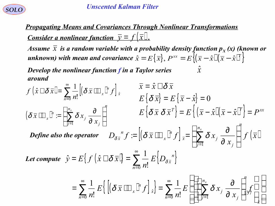
137
Unscented Kalman FilterSOLO
( ) ( )[ ]
( )n
n
j jj
nx
nx
nx
x
xxx
fxn
xxf
∂
∂=∇⋅
∇⋅=+
∑
∑
=
∞
=
1
0ˆ
:
!
1ˆ
δδ
δδ
Develop the nonlinear function f in a Taylor series around
x
Define also the operator ( )[ ] ( )xfx
xfxfD
nn
j jjx
nx
nx
x
∂
∂=∇⋅= ∑=1
: δδδ
Propagating Means and Covariances Through Nonlinear Transformations
Consider a nonlinear function .( )xfy =
Let compute
Assume is a random variable with a probability density function pX (x) (known orunknown) with mean and covariance
x ( ) ( ) Txx xxxxEPxEx ˆˆ,ˆ −−==
( )
( )[ ] ∑ ∑∑
∑∞
= =
∞
=
∞
=
∂
∂=∇⋅=
=+=
0ˆ
10ˆ
0
!
1
!
1
!
1ˆˆ
nx
nn
j jj
nx
nx
n
nx
fx
xEn
fxEn
DEn
xxfEy
x
δδ
δ δ
( ) ( ) xxTT PxxxxExxE
xxExE
xxx
=−−=
=−=+=
ˆˆ
0ˆ
ˆ
δδ
δδ
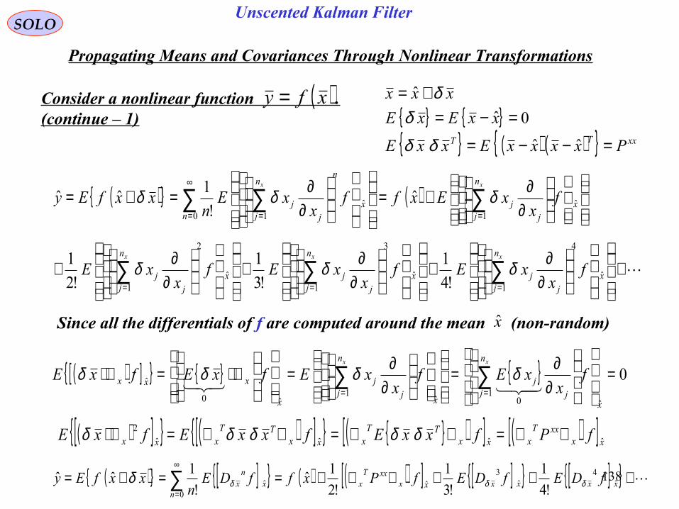
138
Unscented Kalman FilterSOLO
Propagating Means and Covariances Through Nonlinear Transformations
Consider a nonlinear function .(continue – 1)
( )xfy = ( ) ( ) xxTT PxxxxExxE
xxExE
xxx
=−−=
=−=+=
ˆˆ
0ˆ
ˆ
δδ
δδ
( ) ( )
+
∂
∂+
∂
∂+
∂
∂+
∂
∂+=
∂
∂=+=
∑∑∑
∑∑ ∑
===
=
∞
= =
x
n
j jjx
n
j jjx
n
j jj
x
n
j jj
nx
nn
j jj
fx
xEfx
xEfx
xE
fx
xExffx
xEn
xxfEy
xxx
xx
ˆ
4
1ˆ
3
1ˆ
2
1
ˆ10
ˆ1
!4
1
!3
1
!2
1
ˆ!
1ˆˆ
δδδ
δδδ
Since all the differentials of f are computed around the mean (non-random) x
( )[ ] ( )[ ] ( )[ ] ( )[ ]xxxxT
xxxTT
xxxTT
xxx fPfxxEfxxEfxE ˆˆˆˆ2 ∇∇=∇∇=∇∇=∇⋅ δδδδδ
( )[ ] 0
ˆ1
0ˆ1
ˆ0
ˆ =
∂∂=
∂
∂=
∇⋅=∇⋅ ∑∑
==x
n
j jj
x
n
j jj
x
xxx fx
xEfx
xEfxEfxExx
δδδδ
( ) [ ] ( ) ( )[ ] [ ] [ ] +++∇∇+==+= ∑∞
=xxxxxx
xxTx
nx
nx fDEfDEfPxffDE
nxxfEy ˆ
4ˆ
3ˆ
0ˆ
!4
1
!3
1
!2
1ˆ
!
1ˆˆ δδδδ

139
Simon J. Julier
Unscented Kalman FilterSOLO
Propagating Means and Covariances Through Nonlinear Transformations
Consider a nonlinear function .(continue - 2)
( )xfy = ( ) ( ) xxTT PxxxxExxE
xxExE
xxx
=−−=
=−=+=
ˆˆ
0ˆ
ˆ
δδ
δδ
Unscented Transformation (UT), proposed by Julier and Uhlmannuses a set of “sigma points” to provide an approximation ofthe probabilistic properties through the nonlinear function
Jeffrey K. Uhlman
A set of “sigma points” S consists of p+1 vectors and their associatedweights S = i=0,1,..,p: x(i) , W(i) . (1) Compute the transformation of the “sigma points” through the nonlinear transformation f:
( ) ( )( ) pixfy ii ,,1,0 ==(2) Compute the approximation of the mean: ( ) ( )∑
=
≈p
i
ii yWy0
ˆ
The estimation is unbiased if:( ) ( ) ( ) ( ) ( ) yWyyEWyWE
p
i
ip
i y
iip
i
ii ˆˆ00 ˆ0
===
∑∑∑
===
( ) 10
=∑=
p
i
iW
(3) The approximation of output covariance is given by
( ) ( )( ) ( )( )∑=
−−≈p
i
Tiiiyy yyyyWP0
ˆˆ
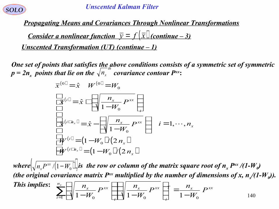
140
Unscented Kalman FilterSOLO
Propagating Means and Covariances Through Nonlinear Transformations
Consider a nonlinear function (continue – 3)( )xfy =
One set of points that satisfies the above conditions consists of a symmetric set of symmetric p = 2nx points that lie on the covariance contour Pxx:
th
xn
( ) ( )
( )
( )
( ) ( ) ( )( ) ( ) ( )
x
xni
xi
xxxni
i
xxxi
ni
nWW
nWW
PW
nxx
PW
nxx
WWxx
x
x ,,1
2/1
2/1
1ˆ
1ˆ
ˆ
0
0
0
0
000
=
−=
−=
−
−=
−
+=
==
+
+
where is the row or column of the matrix square root of nx Pxx /(1-W0)(the original covariance matrix Pxx multiplied by the number of dimensions of x, nx/(1-W0)). This implies:
( )( )i
xxx WPn 01/ −
xxxn
i
T
i
xxx
i
xxx PW
nP
W
nP
W
nx
01 00 111 −=
−
−∑
=
Unscented Transformation (UT) (continue – 1)
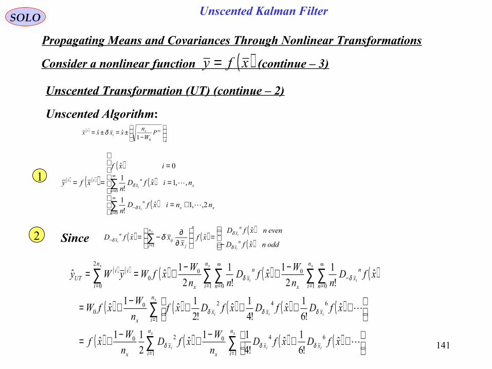
141
Unscented Kalman FilterSOLO
Propagating Means and Covariances Through Nonlinear Transformations
Consider a nonlinear function (continue – 3)( )xfy =
Unscented Transformation (UT) (continue – 2)
( ) ( )( )( )
( )
( )
+=
=
=
==
∑
∑∞
=−
∞
=
0
0
2,,1ˆ!
1
,,1ˆ!
1
0ˆ
nxx
nx
nx
nx
ii
nnixfDn
nixfDn
ixf
xfy
i
i
δ
δ1
2
Unscented Algorithm:
( ) ( ) ( ) ( ) ( )
( ) ( ) ( ) ( ) ( )
( ) ( ) ( ) ( )∑∑
∑
∑ ∑∑ ∑∑
==
=
=
∞
=−
=
∞
==
++−+−+=
++++−+=
−+−+==
x
ii
x
i
x
iii
x
i
x
i
x
n
ixx
x
n
ix
x
n
ixxx
x
n
i n
nx
x
n
i n
nx
x
n
i
iiUT
xfDxfDn
WxfD
n
Wxf
xfDxfDxfDxfn
WxfW
xfDnn
WxfD
nn
WxfWyWy
1
640
1
20
1
64200
1 0
0
1 0
00
2
0
ˆ!6
1ˆ
!4
11ˆ
2
11ˆ
ˆ!6
1ˆ
!4
1ˆ
!2
1ˆ
1ˆ
ˆ!
1
2
1ˆ
!
1
2
1ˆˆ
δδδ
δδδ
δδ
( )
i
xxxi
i PW
nxxxx
−
±=±=01
ˆˆ δ
Since ( ) ( )( )( )
−=
∂
∂−= ∑=
−oddnxfD
evennxfDxf
xxxfD
nx
nx
nn
j jij
nx
i
ix
i ˆ
ˆˆˆ
1 δ
δδ δ

142
Unscented Kalman Filter
( ) ( ) ( ) ( )∑=
++−+∇∇+=
x
ii
n
ixx
x
xxTUT xfDxfD
n
WxfPxfy
1
640 ˆ!6
1ˆ
!4
11ˆ
2
1ˆˆ δδ
( )
i
xxxi
i PW
nxxxx
−
±=±=01
ˆˆ δ
SOLO
Propagating Means and Covariances Through Nonlinear Transformations
Consider a nonlinear function (continue – 4)( )xfy =Unscented Transformation (UT) (continue – 3)
Unscented Algorithm:
( ) ( )
( ) ( ) ( )xfPxfPW
n
n
WxfP
W
nP
W
n
n
W
xfPW
nP
W
n
n
WxfD
n
W
xxTxxxT
x
n
i
T
i
xxx
i
xxxT
x
n
i
T
i
xxx
i
xxxT
x
n
ix
x
x
xx
i
ˆ2
1ˆ
12
11ˆ
112
11
ˆ112
11ˆ
2
11
0
0
1 00
0
1 00
0
1
20
∇∇=∇
−
∇−=∇
−
−
∇−=
∇
−
−
∇−=−
∑
∑∑
=
==δ
Finally:
We found
( ) [ ] ( ) ( )[ ] [ ] [ ] +++∇∇+==+= ∑∞
=xxxxxx
xxTx
nx
nx fDEfDEfPxffDE
nxxfEy ˆ
4ˆ
3ˆ
0ˆ
!4
1
!3
1
!2
1ˆ
!
1ˆˆ δδδδ
We can see that the two expressions agree exactly to the third order.
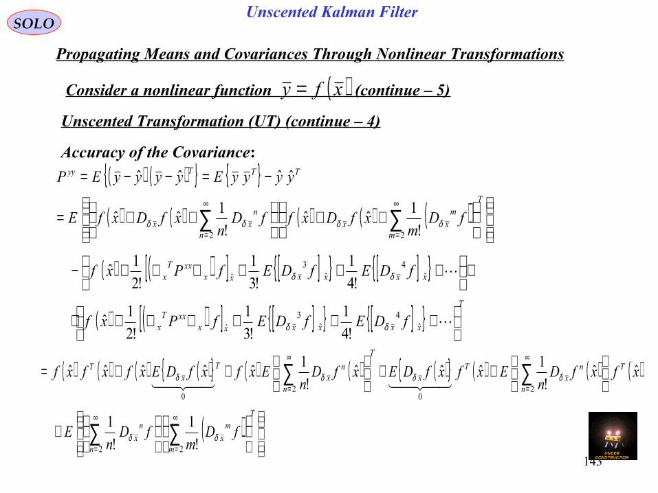
143
Unscented Kalman FilterSOLO
Propagating Means and Covariances Through Nonlinear Transformations
Consider a nonlinear function (continue – 5)( )xfy =Unscented Transformation (UT) (continue – 4)
Accuracy of the Covariance:
( ) ( ) ( ) ( ) ( ) ( ) ( )
( ) ( )[ ] [ ] [ ]
( ) ( )[ ] [ ] [ ] T
xxxxxxxxT
x
xxxxxxxxT
x
T
m
mxx
n
nxx
TTTyy
fDEfDEfPxf
fDEfDEfPxf
fDm
xfDxffDn
xfDxfE
yyyyEyyyyEP
+++∇∇+⋅
⋅
+++∇∇+−
++
++=
−=−−=
∑∑∞
=
∞
=
ˆ4
ˆ3
ˆ
ˆ4
ˆ3
ˆ
22
!4
1
!3
1
!2
1ˆ
!4
1
!3
1
!2
1ˆ
!
1ˆˆ
!
1ˆˆ
ˆˆˆˆ
δδ
δδ
δδδδ
( ) ( ) ( ) ( ) ( ) ( ) ( ) ( ) ( ) ( )
( )
+
++
++=
∑∑
∑∑
∞
=
∞
=
∞
=
∞
=
T
m
mx
n
nx
T
n
nx
Tx
T
n
nx
Tx
T
fDm
fDn
E
xfxfDn
ExfxfDExfDn
ExfxfDExfxfxf
22
20
20
!
1
!
1
ˆˆ!
1ˆˆˆ
!
1ˆˆˆˆˆ
δδ
δδδδ

144
Unscented Kalman FilterSOLO
Propagating Means and Covariances Through Nonlinear Transformations
Consider a nonlinear function (continue – 6)( )xfy =Unscented Transformation (UT) (continue – 5)
Accuracy of the Covariance:( ) ( )
( )[ ] ( )[ ]
( ) ( ) ( )
0
1 1
22
0
1 1
ˆˆ
!2!2
1
!!
1
4
1
ˆˆˆˆ
>
∞
=
∞
=
>
∞
=
∞
=
−
+
∇∇∇∇−=
−=−−=
∑ ∑∑ ∑ji
i j
Tjx
ix
ji
i j
Tjx
ix
T
xxxxT
xxxxxT
xT
xxx
x
TTTyy
fDEfDEji
fDfDji
E
fPfPP
yyyyEyyyyEP
δδδδ
AA
( )[ ] ( )[ ]
( ) ( )
( ) ( ) ( )
0
1 1
2
1
2
1
2~
2~2
2
1
0
1 1
~~
ˆˆ
4!2!2
1
!!
1
2
1
4
1
>
∞
=
∞
= = =
=
>
∞
=
∞
=
+
−
++
∇∇∇∇−=
∑ ∑ ∑ ∑
∑ ∑ ∑
ji
i j
L
k
L
m
Tji
L
k
ji
i j
Tji
T
xxxxT
xxxxxT
xT
xxx
xyy
UT
fDEfDELji
fDfDjiL
fPfPPP
mk
kk
σσ
σσ
λ
λ
AA

145
Uscented Kalman FilterSOLO
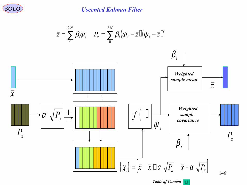
146
Uscented Kalman FilterSOLO
( ) ( )∑∑ −−==N
Tiiiz
N
ii zzPz2
0
2
0
ψψβψβ
x
xPα
xP
zP
( )f
iβ
iβ
iψ
z
[ ]xxi PxPxx ααχ −+=
Weightedsample mean
Weightedsample
covariance
Table of Content

147
Uscented Kalman FilterSOLO
UKF Summary
Initialization of UKF
( ) ( ) TxxxxEPxEx 00000|000 ˆˆˆ −−==
[ ] ( ) ( )
=−−===
R
Q
P
xxxxEPxxExTaaaaaTTaa
00
00
00
ˆˆ00ˆˆ0|0
00000|0000
[ ]TTTTa vwxx =:
For ∞∈ ,,1k
Calculate the Sigma Points ( )( )
λγ
γ
γ +=
=−=
=+=
=
−−−−+
−−
−−−−−−
−−−−
L
LiPxx
LiPxx
xx
ikkkk
Likk
ikkkk
ikk
kkkk
,,1ˆ
,,1ˆ
ˆ
1|11|11|1
1|11|11|1
1|10
1|1
State Prediction and its Covariance
System Definition( ) ( )
==+=
==+−= −−−−−−−
lkkT
lkkkkk
lkkT
lkkkkkk
RvvEvEvxkhz
QwwEwEwuxkfx
,
,1111111
&0,
&0,,1
δ
δ
( ) Liuxkfx ki
kki
kk 2,,1,0,,1 11|11| =−= −−−−
( ) ( ) ( )( ) LiL
WL
WxWx mi
mL
i
ikk
mikk 2,,1
2
1&ˆ 0
2
01|1| =
+=
+== ∑
=−− λλ
λ
0
1
2
( ) ( ) ( ) ( ) ( )( ) LiL
WL
WxxxxWP ci
cL
i
T
kki
kkkki
kkc
ikk 2,,12
1&1ˆˆ 2
0
2
01|1|1|1|1| =
+=+−+
+=−−= ∑
=−−−−− λ
βαλ
λ
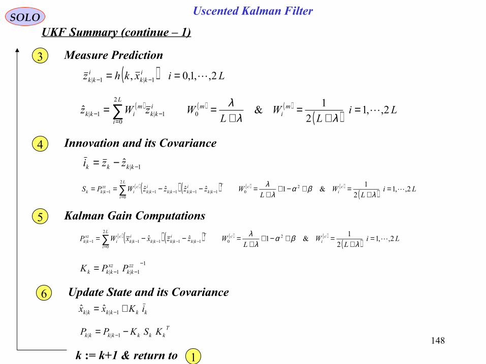
148
Uscented Kalman FilterSOLOUKF Summary (continue – 1)
Measure Prediction
( ) Lixkhz ikk
ikk 2,,1,0, 1|1| == −−
( ) ( ) ( )( ) LiL
WL
WzWz mi
mL
i
ikk
mikk 2,,1
2
1&ˆ 0
2
01|1| =
+=
+== ∑
=−− λλ
λ
3
Innovation and its Covariance4
1|ˆ −−= kkkk zzi
( ) ( ) ( ) ( ) ( )( ) LiL
WL
WzzzzWPS ci
cL
i
T
kki
kkkki
kkc
izzkkk 2,,1
2
1&1ˆˆˆˆ 2
0
2
01|1|1|1|1| =
+=+−+
+=−−== ∑
=−−−−− λ
βαλ
λ
Kalman Gain Computations5( ) ( ) ( ) ( ) ( )
( ) LiL
WL
WzzxxWP ci
cL
i
T
kki
kkkki
kkc
ixzkk 2,,1
2
1&1ˆˆ 2
0
2
01|1|1|1|1| =
+=+−+
+=−−= ∑
=−−−−− λ
βαλ
λ
1
1|1|
−−−= zz
kkxzkkk PPK
Update State and its Covariance6kkkkkk iKxx += −1|| ˆˆ
Tkkkkkkk KSKPP −= −1||
k := k+1 & return to 1

149
Unscented Kalman FilterState Estimation (one cycle)
Sensor DataProcessing andMeasurement
Formation
Observation -to - Track
Association
InputData Track Maintenance
( Initialization,Confirmationand Deletion)
Filtering andPrediction
GatingComputations
Samuel S. Blackman, " Multiple-Target Tracking with Radar Applications", Artech House,1986
Samuel S. Blackman, Robert Popoli, " Design and Analysis of Modern Tracking Systems",Artech House, 1999
SOLO
Simon J. Julier Jeffrey K. Uhlman

150
Uscented Kalman FilterSOLO
Table of Content

151
Numerical Integration Using a Monte Carlo ApproximationSOLO
A Monte Carlo Approximation of the Expected Value Integrals uses Discrete Approximation to the Gaussian PDF ( )xxPxx ,ˆ;N
( )xxPxx ,ˆ;N can be approximated by:
( ) ( ) ( ) ( )∑∑==
−=−≈=ss N
i
i
s
N
i
iixx xxN
xxwPxxx11
1,ˆ; δδNp
We can see that for any x we have
( ) ( )∫∑∫∑∞−
≤∞− =
≈=−x
xx
xxi
ix N
i
ii dPxwdxw
i
s
ττττδ ,ˆ;1
N
The weight wi is not the probability of the point xi. The probability density near xi is given by the density of the points in the region around xi, which can be obtained by a normalized histogram of all xi.
Draw Ns samples from , where xi , i = 1,2,…,Ns are a set of supportpoints (random samples of particles) with weights wi = 1/Ns, i=1,2,…,Ns
( )xxPxx ,ˆ;N
Monte Carlo Kalman Filter (MCKF)
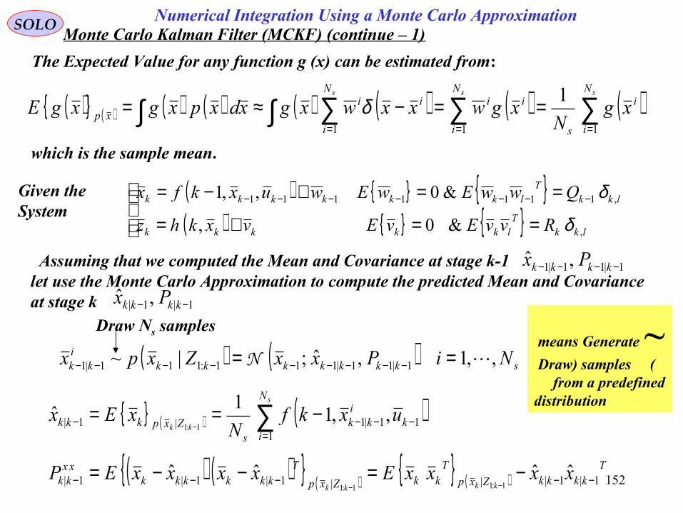
152
Numerical Integration Using a Monte Carlo ApproximationSOLO
The Expected Value for any function g (x) can be estimated from:
( ) ( ) ( ) ( ) ( ) ( ) ( ) ( )∑∑∫ ∑∫===
==−≈=sss N
i
i
s
N
i
iiN
i
iixp xg
NxgwxxwxgxdxpxgxgE
111
1δ
which is the sample mean.
( ) ( )
==+=
==+−= −−−−−−−
lkkT
lkkkkk
lkkT
lkkkkkk
RvvEvEvxkhz
QwwEwEwuxkfx
,
,1111111
&0,
&0,,1
δ
δGiven the System
Assuming that we computed the Mean and Covariance at stage k-1let use the Monte Carlo Approximation to compute the predicted Mean and Covariance at stage k
1|11|1 ,ˆ −−−− kkkk Px
1|1| ,ˆ −− kkkk Px
( ) ( )∑=
−−−− −==−
s
kk
N
ik
ikk
sZxpkkk uxkf
NxEx
111|1|1| ,,1
1ˆ
1:1
( ) ( ) ( ) ( )T
kkkkZxp
TkkZxp
Tkkkkkk
xxkk xxxxExxxxEP
kkkk1|1|||1|1|1| ˆˆˆˆ
1:11:1−−−−− −=−−=
−−
Monte Carlo Kalman Filter (MCKF) (continue – 1)
Draw Ns samples
( ) ( ) skkkkkkki
kk NiPxxZxpx ,,1,ˆ;|~ 1|11|111:111|1 == −−−−−−−−− N~ means Generate
(Draw) samples from a predefined
distribution

153
Numerical Integration Using a Monte Carlo ApproximationSOLO
( ) ( ) ( ) ( )
( )[ ] ( )[ ] ( )
( ) ( ) ( ) ( ) ( )TN
ik
ikk
s
N
ik
ikk
sZxpk
ikk
Tk
ikk
TkkkkZxp
T
kki
kkkki
kk
TkkkkZxp
TkkZxp
Tkkkkkk
xxkk
ss
kk
kk
kkkk
uxkfN
uxkfN
QuxfuxfE
xxwuxkfwuxkfE
xxxxExxxxEP
−
−−+=
−+−+−=
−=−−=
∑∑=
−−−=
−−−−−−−−−
−−−−−−−−−−
−−−−−
−
−
−−
111|1
111|1|11|111|1
1|1||111|1111|1
1|1|||1|1|1|
,,11
,,11
,,
ˆˆ,,1,,1
ˆˆˆˆ
1:1
1:1
1:11:1
( ) ( ) ( ) ( )
−
−−−−+= ∑∑∑
=−−−
=−−−
=−−−−−−−
sss N
ik
ikk
s
N
ik
ikk
s
N
ik
ikk
Tk
ikk
s
xxkk uxkf
Nuxkf
Nuxkfuxkf
NQP
111|1
111|1
111|111|11| ,,1
1,,1
1,,1,,1
1
Using the Monte Carlo Approximation we obtain:
( ) ( )∑=
−− ==−
s
kk
N
i
ikk
sZxpkkk xkh
NzEz
11||1| ,
1ˆ
1:1
( ) ( ) ( ) ( )
−+= ∑∑∑
=−
=−
=−−−
sss N
i
ikk
s
N
i
ikk
s
N
i
ikk
Tikk
s
zzkk xkh
Nxkh
Nxkhxkh
NRP
11|
11|
11|1|1| ,
1,
1,,
1
Monte Carlo Kalman Filter (MCKF) (continue – 2)
( ) ( ) skkkkkkki
kk NiPxxZxpx ,,1,ˆ;|~ 1|1|1:11| == −−−− N
Now we approximate the predictive PDF, , as and we draw new Ns (not necessarily the same as before) samples.
( )1:1| −kk Zxp ( )1|1| ,ˆ; −− kkkkk PxxN

154
Numerical Integration Using a Monte Carlo ApproximationSOLO
In the same way we obtain:
( ) ( )
−= ∑∑∑
=−
=−
=−−−
sss N
i
ikk
s
N
i
ikk
s
N
i
ikk
Tikk
s
zxkk xkh
Nx
Nxkhx
NP
11|
11|
11|1|1| ,
11,
1
Monte Carlo Kalman Filter (MCKF) (continue – 3)
The Kalman Filter Equations are:
( ) 11|1|
−−−= zz
kkzx
kkk PPK
( )1|1|| ˆˆˆ −− −+= kkkkkkkk zzKxx
Tk
zzkkk
xxkk
xxkk KPKPP 1|1|| −− −=
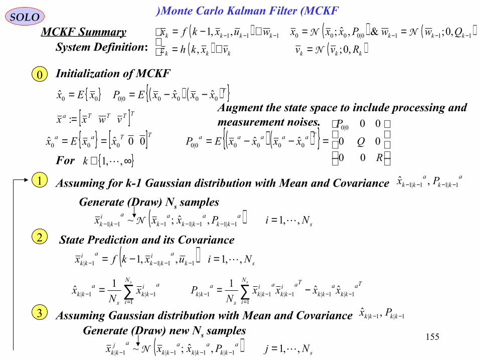
155
Monte Carlo Kalman Filter (MCKF)SOLOMCKF Summary
( ) ( ) TxxxxEPxEx 00000|000 ˆˆˆ −−==
[ ] ( ) ( )
=−−===
R
Q
P
xxxxEPxxExTaaaaaTTaa
00
00
00
ˆˆ00ˆˆ0|0
00000|0000
For ∞∈ ,,1k
System Definition:( ) ( ) ( )( ) ( )
=+===+−= −−−−−−
kkkkkk
kkkkkkk
Rvvvxkhz
QwwPxxxwuxkfx
,0;,
,0;&,ˆ;,,1 1110|0000111
N
NN
( ) sk
aikk
aikk Niuxkfx ,,1,,1 11|11| =−= −−−−
∑=
−− =sN
i
aikk
s
akk x
Nx
11|1|
1ˆ
Initialization of MCKF0
State Prediction and its Covariance2
Takk
akk
N
i
Taikk
aikk
s
akk xxxx
NP
s
1|1|1
1|1|1| ˆˆ1
−−=
−−− −= ∑
Assuming for k-1 Gaussian distribution with Mean and Covariance1 akk
akk Px 1|11|1 ,ˆ −−−−
Assuming Gaussian distribution with Mean and Covariance3 1|1| ,ˆ −− kkkk Px
( ) sa
kka
kka
k
aikk NiPxxx ,,1,ˆ;~ 1|11|111|1 =−−−−−−− N
Generate (Draw) Ns samples
( ) sa
kka
kka
kk
ajkk NjPxxx ,,1,ˆ;~ 1|1|1|1| =−−−− N
Generate (Draw) new Ns samples
[ ]TTTTa vwxx =:Augment the state space to include processing and measurement noises.
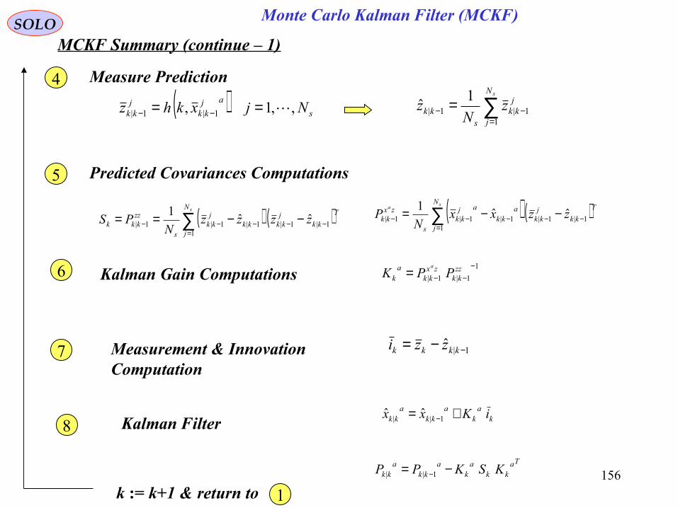
156
Monte Carlo Kalman Filter (MCKF)SOLOMCKF Summary (continue – 1)
( ) s
ajkk
jkk Njxkhz ,,1, 1|1| == −− ∑
=−− =
sN
j
jkk
skk z
Nz
11|1|
1ˆ
Measure Prediction4
( ) ( )∑=
−−−−− −−==sN
j
T
kkjkkkk
jkk
s
zzkkk zzzz
NPS
11|1|1|1|1| ˆˆ
1
Measurement & InnovationComputation
1|ˆ −−= kkkk zzi7
( ) ( )∑=
−−−−− −−=sa
N
j
T
kkjkk
akk
ajkk
s
zxkk zzxx
NP
11|1|1|1|1| ˆˆ
1
6 Kalman Gain Computations1
1|1|
−−−= zz
kkzx
kka
k PPKa
Kalman Filter8k
ak
akk
akk iKxx += −1|| ˆˆ
Takk
ak
akk
akk KSKPP −= −1||
k := k+1 & return to 1
Predicted Covariances Computations5

157
Sensor DataProcessing andMeasurement
Formation
Observation -to - Track
Association
InputData Track Maintenance
( Initialization,Confirmationand Deletion)
Filtering andPrediction
GatingComputations
Samuel S. Blackman, " Multiple-Target Tracking with Radar Applications", Artech House,1986
Samuel S. Blackman, Robert Popoli, " Design and Analysis of Modern Tracking Systems",Artech House, 1999
SOLO Monte Carlo Kalman Filter (MCKF)
Table of Content

158
Nonlinear Estimation Using Particle FiltersSOLO
We assumed that p (xk|Z1:k) is a Gaussian PDF. If the true PDF is not Gaussian (multivariate, heavily skewed or non-standard – not represented by any standard PDF) the Gaussian distribution can never described it well.
Non-Additive Non-Gaussian Nonlinear Filter
( )( )kkk
kkk
vxhz
wxfx
,
, 11
== −−
kk vw &1− are system and measurement white-noise sequencesindependent of past and current states and on each other andhaving known P.D.F.s ( ) ( )kk vpwp &1−
We want to compute p (xk|Z1:k) recursively, assuming knowledge of p(xk-1|Z1:k-1) in two stages, prediction (before) and update (after measurement)
Prediction (before measurement)Use Chapman – Kolmogorov Equation to obtain:
( ) ( ) ( )∫ −−−−− = 11:1111:1 ||| kkkkkkk xdZxpxxpZxp
where: ( ) ( ) ( )∫ −−−−−− = 111111 |,|| kkkkkkkk wdxwpwxxpxxp
By assumption ( ) ( )111 | −−− = kkk wpxwp
Since by knowing , is deterministically given by system equation
we have
11 & −− kk wx kx
( ) ( )( ) ( )( )
≠=
=−=−−
−−−−−−
11
111111 ,0
,1,,|
kkk
kkkkkkkkk wxfx
wxfxwxfxwxxp δ
Therefore: ( ) ( )( ) ( )∫ −−−−− −= 11111 ,| kkkkkkk wdwpwxfxxxp δ

159
Nonlinear Estimation Using Particle FiltersSOLO Non-Additive Non-Gaussian Nonlinear Filter
( )( )kkk
kkk
vxhz
wxfx
,
, 11
== −−
kk vw &1− are system and measurement white-noise sequencesindependent of past and current states and on each other andhaving known P.D.F.s ( ) ( )kk vpwp &1−
We want to compute p (xk|Z1:k) recursively, assuming knowledge of p(xk-1|Z1:k-1) in two stages, prediction (before) and update (after measurement)
Prediction (before measurement)
( ) ( ) ( )∫ −−−−− = 11:1111:1 ||| kkkkkkk xdZxpxxpZxp
where:
( ) ( )( ) ( ) ( )
( )
( ) ( )( )
( ) ( )( ) ( )∫ −
−
−
−
=− ===
kkkkk
kkkk
kk
kkkkBayes
bp
apabpbap
kkkkkxdZxpxzp
Zxpxzp
Zzp
ZxpxzpZzxpZxp
1:1
1:1
1:1
1:1
||
1:1:1||
||
|
||,||
( ) ( ) ( )∫= kkkkkkkk vdxvpvxzpxzp |,||
By assumption ( ) ( )kkk vpxvp =|
Since by knowing , is deterministically given by system equationkk vx & kz
( ) ( )( ) ( )( )
≠=
=−=kkk
kkkkkkkkk vxhz
vxhzvxhzvxzp
,0
,1,,| δ
Therefore: ( ) ( )( ) ( )∫ −= kkkkkkk vdvpvxhzxzp ,| δ
( ) ( )( ) ( )∫ −−−−− −= 11111 ,| kkkkkkk wdwpwxfxxxp δ
1
Update (after measurement)2

160
Nonlinear Estimation Using Particle FiltersSOLO Non-Additive Non-Gaussian Nonlinear Filter
( )( )kkk
kkk
vxhz
wxfx
,
, 11
== −−
kk vw &1− are system and measurement white-noise sequencesindependent of past and current states and on each other andhaving known P.D.F.s ( ) ( )kk vpwp &1−
We want to compute p (xk|Z1:k) recursively, assuming knowledge of p(xk-1|Z1:k-1) in two stages, prediction (before) and update (after measurement)
Prediction (before measurement) ( ) ( ) ( )∫ −−−−− = 11:1111:1 ||| kkkkkkk xdZxpxxpZxp
( ) ( )( ) ( )∫ −−−−− −= 11111 ,| kkkkkkk wdwpwxfxxxp δ
Update (after measurement)
( ) ( )( ) ( ) ( )
( )
( ) ( )( )
( ) ( )( ) ( )∫ −
−
−
−
=− ===
kkkkk
kkkk
kk
kkkkBayes
bp
apabpbap
kkkkkxdZxpxzp
Zxpxzp
Zzp
ZxpxzpZzxpZxp
1:1
1:1
1:1
1:1
||
1:1:1||
||
|
||,||
We need to evaluate the following integrals:
( ) ( )( ) ( )∫ −= kkkkkkk vdvpvxhzxzp ,| δ
We use the numeric Monte Carlo Method to evaluate the integrals:
Generate (Draw): ( ) ( ) Skikk
ik Nivpvwpw ,,1~&~ 11 =−−
( ) ( )( ) S
N
i
ik
ik
ikkk Nwxfxxxp
S
∑=
−−− −≈1
111 /,| δ
( ) ( )( ) S
N
i
ik
ik
ikkk Nvxhzxzp
S
∑=
−≈1
/,| δor
( ) ( ) ( ) S
N
i
ikkkk
ik
ik
ik Nxxxxpwxfx
S
∑=
−−− −≈→=1
111 /|, δ
( ) ( ) ( ) S
N
i
ikkkk
ik
ik
ik Nzzxzpvxhz
S
∑=
−≈→=1
/|, δ
Analytic solutions for those integralequations do not exist in the generalcase.
12

161
SOLO
( ) ( ) ( )( ) ( )kvkkk
xkkwkkkk
vpgivenvxhz
xpuwpgivenwuxfx
:,
,,:,, 011111 0
=
= −−−−−
Monte Carlo Computations of and . ( )kk xzp |( )1| −kk xxp
Generate (Draw) ( ) Sxi Nixpx ,,1~ 00 0
=For ∞∈ ,,1 k
Initialization0
1 At stage k-1
Generate (Draw) NS samples ( ) Skwik Niwpw ,,1~ 11 =−−
2 State Update ( ) Sikk
ik
ik Niwuxfx ,,1,, 111 == −−−
3 Generate (Draw) Measurement Noise ( ) Skvik Nivpv ,,1~ =
k:=k+1 & return to 1
( ) ( )∑=
− −≈SN
iS
ikkkk Nxxxxp
11 /| δ
( ) ( )∑=
−≈SN
iS
ikkkk Nzzxzp
1
/| δ
4 Measurement , Update ( ) Sik
ik
ik Nivxhz ,,1, ==kz
Nonlinear Estimation Using Particle FiltersNon-Additive Non-Gaussian Nonlinear Filter

162
Nonlinear Estimation Using Particle FiltersSOLO Non-Additive Non-Gaussian Nonlinear Filter
( )( )kkk
kkk
vxhz
wxfx
,
, 11
== −−
kk vw &1− are system and measurement white-noise sequencesindependent of past and current states and on each other andhaving known P.D.F.s ( ) ( )kk vpwp &1−
We want to compute p (xk|Z1:k) recursively, assuming knowledge of p(xk-1|Z1:k-1) in two stages, prediction (before) and update (after measurement)
Prediction (before measurement) ( ) ( ) ( )∫ −−−−− = 11:1111:1 ||| kkkkkkk xdZxpxxpZxp
Update (after measurement)
( ) ( )( ) ( ) ( )
( )
( ) ( )( )
( ) ( )( ) ( )∫ −
−
−
−
=− ===
kkkkk
kkkk
kk
kkkkBayes
bp
apabpbap
kkkkkxdZxpxzp
Zxpxzp
Zzp
ZxpxzpZzxpZxp
1:1
1:1
1:1
1:1
||
1:1:1||
||
|
||,||
We use the numeric Monte Carlo Method to evaluate the integrals:
Generate (Draw): ( ) ( ) Skikk
ik Nivpvwpw ,,1~&~ 11 =−−
( ) ( ) ( ) S
N
i
ikkkk
ik
ik
ik Nxxxxpwxfx
S
∑=
−−− −≈→=1
111 /|, δ
( ) ( ) ( ) S
N
i
ikkkk
ik
ik
ik Nzzxzpvxhz
S
∑=
−≈→=1
/|, δ
( ) ( ) ( ) ( ) ( ) ( )∑∑ ∫∫ ∑==
−−−−=
−−− −=−=−=SSS N
i
ikk
S
N
ikkk
ikk
Sk
N
ikk
ikk
Skk xx
NxdZxpxx
NxdZxpxx
NZxp
111
11:1111
1:111:1
1|
1|
1| δδδ
Since we use NS points to describe the probabilities wecall those points, Particles.
12
Table of Content
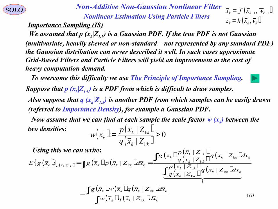
163
Nonlinear Estimation Using Particle FiltersSOLO
We assumed that p (xk|Z1:k) is a Gaussian PDF. If the true PDF is not Gaussian (multivariate, heavily skewed or non-standard – not represented by any standard PDF) the Gaussian distribution can never described it well. In such cases approximate Grid-Based Filters and Particle Filters will yield an improvement at the cost of heavy computation demand.
( ) ( )( ) 0
|
|:
:1
:1 >=kk
kkk Zxq
Zxpxw
To overcome this difficulty we use The Principle of Importance Sampling.
Suppose that p (xk|Z1:k) is a PDF from which is difficult to draw samples.
Also suppose that q (xk|Z1:k) is another PDF from which samples can be easily drawn(referred to Importance Density), for example a Gaussian PDF.
Now assume that we can find at each sample the scale factor w (xk) between the two densities:
Using this we can write:
( ) ( ) ( ) ( )( ) ( )
( ) ( )( )( ) ( )
( ) ( ) ( )( ) ( )∫
∫
∫
∫∫
=
==
kkkk
kkkkk
kkkkk
kk
kkkkk
kkk
kkkkZxpk
xdZxqxw
xdZxqxwxg
xdZxqZxqZxp
xdZxqZxq
Zxpxg
xdZxpxgxgEkk
:1
:1
1
:1:1
:1
:1:1
:1
:1|
|
|
|||
||
|
|:1
Non-Additive Non-Gaussian Nonlinear Filter ( )( )kkk
kkk
vxhz
wxfx
,
, 11
== −−
Importance Sampling (IS)
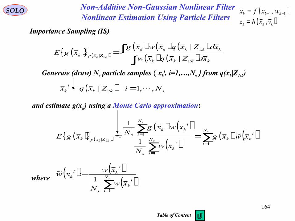
164
SOLO
( ) ( )( ) ( ) ( )
( ) ( )∫∫=
kkkk
kkkkk
ZxpkxdZxqxw
xdZxqxwxgxgE
kk
:1
:1
||
|:1
( ) ( )( )∑
=
=sN
i
ik
s
iki
k
xwN
xwxw
1
1:~
where
Generate (draw) Ns particle samples xki, i=1,…,Ns from q(xk|Z1:k)
( ) skki
k NiZxqx ,,1|~ :1 =
( ) ( )
( ) ( )( )
( ) ( )∑∑
∑=
=
= =≈s
s
s
kk
N
i
ikkN
i
ik
s
N
i
ikk
sZxpk xwxg
xwN
xwxgN
xgE1
1
1|
~1
1
:1
and estimate g(xk) using a Monte Carlo approximation:
Nonlinear Estimation Using Particle FiltersNon-Additive Non-Gaussian Nonlinear Filter ( )
( )kkk
kkk
vxhz
wxfx
,
, 11
== −−
Importance Sampling (IS)
Table of Content

165
SOLO
It would be useful if the importance density could be generated recursively (sequentially).
( ) ( )( ) ( ) ( ) ( )
( )
( ) ( ) ( )( )
( ) ( ) ( )( )kk
kkkkZzpc
kk
kkkkkk
bP
aPabPbaP
Bayes
kk
kkkk Zxq
Zxpxzpc
Zxq
ZzpZxpxzp
Zxq
Zzxpxw
kk
:1
1:1|/1:
:1
1:11:1
||:1
1:1
|
||
|
|/||
|
,| 1:1−
=−−
=
−−
===
( )( ) ( ) ( )
( ) ( )1:111:11|,
1:11 |,||, −−−−=−− = kkkkkbPbaPbaP
Bayes
kkk ZxpZxxpZxxp
( ) ( ) ( ) ( )∫∫ −−−−−−−−− == 11:111:1111:111:1 |,||,| kkkkkkkkkkkk xdZxpZxxpxdZxxpZxp
Using:
we obtain:
( ) ( ) ( ) ( )∫∫ −−−−−−−−− == 11:111:1111:111:1 |,||,| kkkkkkkkkkkk xdZxqZxxqxdZxxqZxq
In the same way:
( ) ( ) ( )( )
( ) ( ) ( )( ) ( )∫
∫−−−−−
−−−−−− ==11:111:11
11:111:11
:1
1:1
|,|
|,||
|
||
kkkkkk
kkkkkkkk
kk
kkkkk
xdZxqZxxq
xdZxpZxxpxzpc
Zxq
Zxpxzpcxw
Sequential Importance Sampling (SIS)
Nonlinear Estimation Using Particle FiltersNon-Additive Non-Gaussian Nonlinear Filter ( )
( )kkk
kkk
vxhz
wxfx
,
, 11
== −−

166
SOLO
It would be useful if the importance density could be generated recursively.
( ) ( ) ( )( )
( ) ( ) ( )( ) ( )∫
∫−−−−−
−−−−−− ==11:111:11
11:111:11
:1
1:1
|,|
|,||
|
||
kkkkkk
kkkkkkkk
kk
kkkkk
xdZxqZxxq
xdZxpZxxpxzpc
Zxq
Zxpxzpcxw
Suppose that at k-1 we have Ns particle samples and their probabilities xk-1|k-1
i,wk-1i ,i=1,…,Ns , that constitute a random measure which characterizes the
posterior PDF for time up to tk-1. Then
( ) ( ) ( )∑=
−−−−−−−− −≈sN
i
ikkkk
ikkkk xxZxpZxp
11|111:11|11:11 || δ
( )( ) ( ) ( ) ( )
( ) ( ) ( )∫ ∑
∫ ∑
=−−−−−−−−
−=
−−−−−−−−
−
−=
s
s
N
i
ikkkk
ikkkkk
k
N
i
ikkkk
ikkkkkkk
k
xxZxqZxxq
xdxxZxpZxxpxzpcxw
11|111:11|11:11
11
1|111:11|11:11
|,|
|,||
δ
δ
( ) ( ) ( )∑=
−−−−−−−− −≈sN
i
ikkkk
ikkkk xxZxqZxq
11|111:11|11:11 || δ
Sequential Importance Sampling (SIS) (continue – 1)
We obtained:
Nonlinear Estimation Using Particle FiltersNon-Additive Non-Gaussian Nonlinear Filter ( )
( )kkk
kkk
vxhz
wxfx
,
, 11
== −−

167
SOLO
( ) ( )( )
( ) ( )( )kk
kkkkBayes
kk
kkk Zxq
Zxpxzpc
Zxq
Zxpxw
:1
1:1
:1
:1
|
||
|
| −==
( )( ) ( ) ( ) ( )
( ) ( ) ( )( ) ( ) ( )
( ) ( )
( ) ( )( ) ( ) ( ) ( ) ( )
( ) ( )1:11|11|1
1:11|11|1|,|
|,|
1:11|11:11|1
1:11|11:11|1
11|111:11|11:11
11
1|111:11|11:11
||
|||
|,|
|,||
|,|
|,||
1|11:11|1
1|11:11|1 −−−−−
−−−−−=
=
−−−−−−
−−−−−−
=−−−−−−−−
−=
−−−−−−−−
−−−−−
−−−−−
=
=
−
−=
∫ ∑
∫ ∑
ki
kki
kkk
ki
kki
kkkkkxxpZxxp
xxqZxxq
ki
kkki
kkk
ki
kkki
kkkkk
N
i
ikkkk
ikkkkk
k
N
i
ikkkk
ikkkkkkk
k
Zxqxxq
Zxpxxpxzpc
ZxqZxxq
ZxpZxxpxzpc
xxZxqZxxq
xdxxZxpZxxpxzpcxw
ikkkk
ikkk
ikkkk
ikkk
s
s
δ
δ
( ) ( )( )1:11
1:111 |
|
−−
−−− =
kk
kkk Zxq
ZxpxwSince
( ) ( )( )i
kkikk
ikk
ikk
ikkki
kik xxq
xxpxzpcww
1|1|
1|1||1 |
||
−−
−−−=
Define ( ) ( )( )k
ikk
kikki
kkik Zxq
Zxpxww
:1|
:1|| |
|: ==
( ) ( )( )1:11|1
1:11|11|11 |
|:
−−−
−−−−−− ==
ki
kk
ki
kkikk
ik Zxq
Zxpxww
Sequential Importance Sampling (SIS) (continue – 2)Nonlinear Estimation Using Particle FiltersNon-Additive Non-Gaussian Nonlinear Filter ( )
( )kkk
kkk
vxhz
wxfx
,
, 11
== −−

168
SOLO
Sequential Importance Sampling (SIS) (continue – 3)
( ) ( )
( )( ) ( ) ( )( )( ) ( )( ) twwwt
Zxxq
xxpxzpww i
kk
N
i
ik
kik
ik
ik
ik
ikk
N
ik
ik /~~
,|
||~~1:11
1
/1
1 ==→= ∑=−
−−
( ) ( )∑=
−− −=≈
N
i
ikk
ikkk NxxNxZxp
1
11:1 /:,| δ
k:=k+1Run This
Nonlinear Estimation Using Particle FiltersNon-Additive Non-Gaussian Nonlinear Filter ( )
( )kkk
kkk
vxhz
wxfx
,
, 11
== −−
( ) ( )∑=
−=N
i
ikk
ikkk xxwZxp
1:1| δ
Generate (Draw) ( ) Sxi Nixpx ,,1~ 00 0
=For ∞∈ ,,1 k
Initialization0
1 At stage k-1
Generate (Draw) NS samples ( ) Skwik Niwpw ,,1~ 11 =−−
2 State Update ( ) Sikk
ik
ik Niwuxfx ,,1,, 111 == −−−
Start with the approximation ( ) ( )∑=
− −≈SN
iS
ikkkk Nxxxxp
11 /| δ3
After measurement zk we compute ( ) ( ) ( ) ik
ikkk wxZxp ~,| :1 ≈4
Generate (Draw) NS samples ( ) Skwik Nivpv ,,1~ =
Compute ( )ikik
ik vxhz ,=
Approximate ( ) ( )∑=
−=SN
iS
ikk
ikk Nzzxzp
1
/| δ
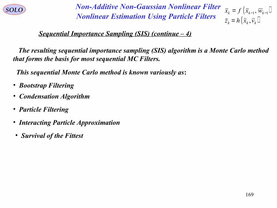
169
SOLO
The resulting sequential importance sampling (SIS) algorithm is a Monte Carlo methodthat forms the basis for most sequential MC Filters.
Sequential Importance Sampling (SIS) (continue – 4)
This sequential Monte Carlo method is known variously as:
• Bootstrap Filtering
• Condensation Algorithm
• Particle Filtering
• Interacting Particle Approximation
• Survival of the Fittest
Nonlinear Estimation Using Particle FiltersNon-Additive Non-Gaussian Nonlinear Filter ( )
( )kkk
kkk
vxhz
wxfx
,
, 11
== −−
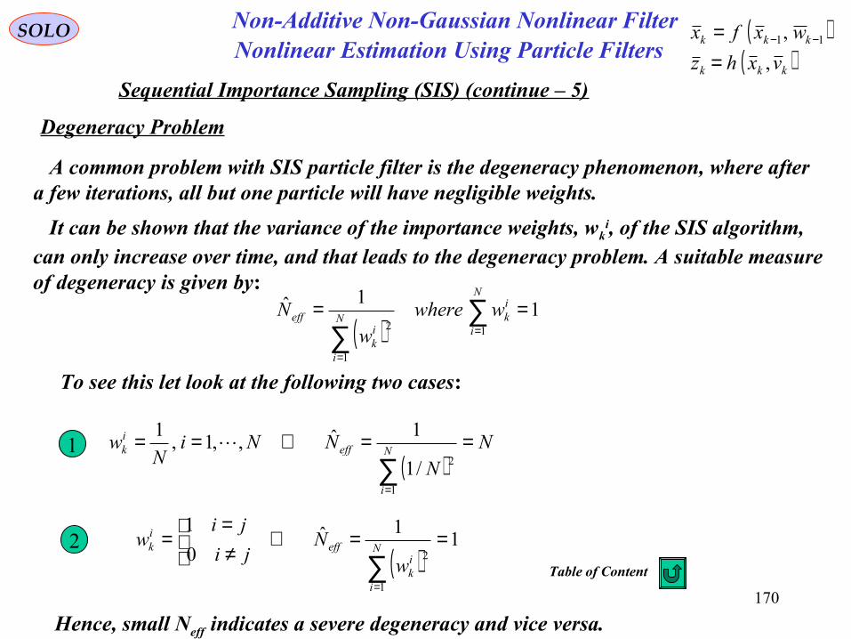
170
SOLO
Degeneracy Problem
Sequential Importance Sampling (SIS) (continue – 5)
A common problem with SIS particle filter is the degeneracy phenomenon, where aftera few iterations, all but one particle will have negligible weights.
It can be shown that the variance of the importance weights, wki, of the SIS algorithm,
can only increase over time, and that leads to the degeneracy problem. A suitable measureof degeneracy is given by:
( )1
1ˆ1
1
2== ∑
∑ =
=
N
i
ikN
i
ik
eff wwherew
N
To see this let look at the following two cases:
1( )
NN
NNiN
w N
i
effik ==⇒==
∑=1
2/1
1ˆ,,1,1
2( )
11ˆ
0
1
1
2==⇒
≠=
=∑
=
N
i
ik
effik
wN
ji
jiw
Hence, small Neff indicates a severe degeneracy and vice versa.
Nonlinear Estimation Using Particle FiltersNon-Additive Non-Gaussian Nonlinear Filter ( )
( )kkk
kkk
vxhz
wxfx
,
, 11
== −−
Table of Content
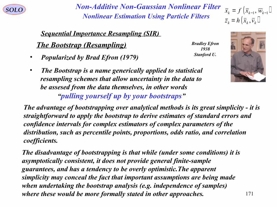
171
SOLO
The Bootstrap (Resampling)
• Popularized by Brad Efron (1979)
• The Bootstrap is a name generically applied to statistical resampling schemes that allow uncertainty in the data to be assesed from the data themselves, in other words
“pulling yourself up by your bootstraps”
The disadvantage of bootstrapping is that while (under some conditions) it is asymptotically consistent, it does not provide general finite-sample guarantees, and has a tendency to be overly optimistic.The apparent simplicity may conceal the fact that important assumptions are being made when undertaking the bootstrap analysis (e.g. independence of samples) where these would be more formally stated in other approaches.
The advantage of bootstrapping over analytical methods is its great simplicity - it is straightforward to apply the bootstrap to derive estimates of standard errors and confidence intervals for complex estimators of complex parameters of the distribution, such as percentile points, proportions, odds ratio, and correlation coefficients.
Sequential Importance Resampling (SIR)
Nonlinear Estimation Using Particle FiltersNon-Additive Non-Gaussian Nonlinear Filter ( )
( )kkk
kkk
vxhz
wxfx
,
, 11
== −−
Bradley Efron1938
Stanford U.

172
SOLO
Resampling
Sequential Importance Resampling (SIR) (continue – 1)
Whenever a significant degeneracy is observed (i.e., when Neff falls bellow someThreshold Nthr) during the sampling, where we obtained
( ) ( )∑=
−≈N
i
ikk
ikkk xxwZxp
1:1| δ
we need to resample and replace the mapping representation with a random measure
Niwx ik
ik ,,1, =
NiNx ik ,,1/1,* =This is done by first computing the Cumulative Density Function (C.D.F.) of thesampled distribution wk
i.
Initialize the C.D.F.: c1 = wk1
Compute the C.D.F.: ci = ci-1 + wki
For i = 2:N
i := i + 1
Nonlinear Estimation Using Particle FiltersNon-Additive Non-Gaussian Nonlinear Filter ( )
( )kkk
kkk
vxhz
wxfx
,
, 11
== −−
173
SOLO
Resampling (continue – 1)
Sequential Importance Resampling (SIR) (continue – 2)
Using the method of Inverse Transform Algorithm we generate N independent and identical distributed (i.i.d.) variables from the uniform distribution u, we sort them in ascending order and we compare them with the Cumulative Distribution Function (C.D.F.)of the normalized weights.
Nonlinear Estimation Using Particle FiltersNon-Additive Non-Gaussian Nonlinear Filter ( )
( )kkk
kkk
vxhz
wxfx
,
, 11
== −−
Non-Additive Non-Gaussian Nonlinear Filter ( )( )kkk
kkk
vxhz
wxfx
,
, 11
== −−

174
SOLO
Resampling Algorithm (continue – 2)Sequential Importance Resampling (SIR) (continue – 3)
Initialize the C.D.F.: c1 = wk1
Compute the C.D.F.: ci = ci-1 + wki
For i = 2:N
i := i + 1
0
Start at the bottom of the C.D.F.: i = 1
Draw for the uniform distribution [ ]1,0~ −NUui
1 For i=1:N
Move along the C.D.F. uj = ui +(j – 1) N-1.
For j=1:N2
WHILE uj > ci
j* = i + 1END WHILE
3
END For
5 i := i + 1 If i < N Return to 1
4 Assign sample: ik
jk xx =*
Assign weight:1−= Nw j
k Assign parent: ii j =
Nonlinear Estimation Using Particle FiltersNon-Additive Non-Gaussian Nonlinear Filter ( )
( )kkk
kkk
vxhz
wxfx
,
, 11
== −−

175
SOLO
Resampling
Sequential Importance Resampling (SIR) (continue – 4)
( ) ( )
( )( ) ( ) ( )( )( ) ( )( )
twwwt
Zxxq
xxpxzpww
ikk
N
i
ik
kik
ik
ik
ik
ikk
N
ik
ik
/~~
,|
||~~
1
:11
1
/1
1
==
=
∑=
−
−−
After measurement zk-1 wecompute ( ) ( ) ( ) i
kikkk wxZxp ~,| :1 ≈
1
Start with the approximation
( ) ( )∑
=
−−
−=
≈N
i
ikk
ikkk
Nxx
NxZxp
1
11:1
/:
,|
δ
0
Prediction( ) ( ) ( )( )i
kkik
ik nuxfx ,,*1 =+
to obtain ( ) ( ) 11:11 ,| −
++ ≈ NxZxp ikkk
3
k:=k+1 Run This
Nonlinear Estimation Using Particle FiltersNon-Additive Non-Gaussian Nonlinear Filter ( )
( )kkk
kkk
vxhz
wxfx
,
, 11
== −−
( ) ( )∑=
−=N
i
ikk
ikkk xxwZxp
1:1| δ
If Resample to obtain ( ) ( ) 1
:1 ,*| −≈ NxZxp ikkk
2 ( ) tht
N
i
ikeff NwN <
= ∑
=1
2/1

176
SOLO
Resampling
Sequential Importance Resampling (SIR) (continue – 5)
Although the resampling step reduces the effect of degeneracy, it introduces otherpractical problems:
It limits the possibility of parallel implementation.
The particles that have high wki are statistically selected many times. This leads to
loss of diversity among the particles (sample impoverishment).
1
2
Several other techniques for generating samples from an unknown P.D.F., besideImportance Sampling, have been presented in the literature. If the P.D.F. is stationary,Markov Chain Monte Carlo (MCMC) methods have been proposed:• Metropolis – Hastings (MH)• Gibbs sampler (a special case of MH) (see Probability Presentation)
Nonlinear Estimation Using Particle FiltersNon-Additive Non-Gaussian Nonlinear Filter ( )
( )kkk
kkk
vxhz
wxfx
,
, 11
== −−
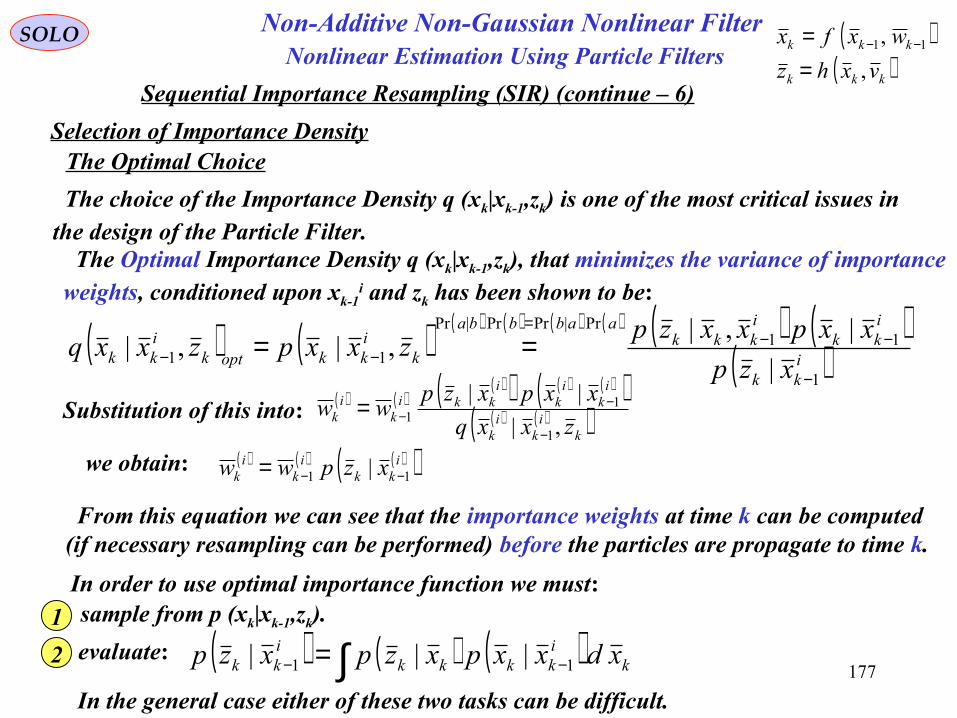
177
SOLO
Selection of Importance Density
Sequential Importance Resampling (SIR) (continue – 6)
The choice of the Importance Density q (xk|xk-1,zk) is one of the most critical issues inthe design of the Particle Filter.
The Optimal Choice
The Optimal Importance Density q (xk|xk-1,zk), that minimizes the variance of importanceweights, conditioned upon xk-1
i and zk has been shown to be:
( ) ( ) ( ) ( ) ( ) ( ) ( ) ( )( )i
kk
ikk
ikkk
aabbba
kikkoptk
ikk xzp
xxpxxzpzxxpzxxq
1
11Pr|PrPr|Pr
11 |
|,|,|,|
−
−−=
−− ==
( ) ( )( )( ) ( ) ( )( )( ) ( )( )k
ik
ik
ik
ik
ikki
ki
k zxxq
xxpxzpww
,|
||
1
11
−
−−= Substitution of this into:
we obtain: ( ) ( ) ( )( )ikk
ik
ik xzpww 11 | −−=
From this equation we can see that the importance weights at time k can be computed(if necessary resampling can be performed) before the particles are propagate to time k.
In order to use optimal importance function we must: sample from p (xk|xk-1,zk).1
evaluate:2 ( ) ( ) ( )∫ −− = kikkkk
ikk xdxxpxzpxzp 11 |||
In the general case either of these two tasks can be difficult.
Nonlinear Estimation Using Particle FiltersNon-Additive Non-Gaussian Nonlinear Filter ( )
( )kkk
kkk
vxhz
wxfx
,
, 11
== −−

178
Sequential Importance Resampling Particle Filter (SIRPF)SOLOSIRPF Summary
Initialization of SIRPF
( )00 0~ˆ xpx x
For ∞∈ ,,1 k
Assuming for k-1 Gaussian distribution with Mean and Covariance
( ) skkkkki
kk NiPxxx ,,1,ˆ;ˆ 1|11|111|1 == −−−−−−− N
State Prediction and its Covariance
System Definition( ) ( ) ( )( ) ( )
=
−= −−−
kvkkkk
kwkxkkkk
vpvvxkhz
wpwxpxwuxkfx
~,,
~,~,,,1 00111 0
( ) ski
kkikk Niuxkfx ,,1,,1 11|11| =−= −−−−
0
1
2
1|11|1 ,ˆ −−−− kkkk Px
Generate Ns samples
Assuming Gaussian distribution with Mean and Covariance
( ) skkkkkkjkk NjPxxx ,,1,ˆ; 1|1|1|1| == −−−− N
3 1|1| ,ˆ −− kkkk Px
Generate new Ns samples
Draw
Table of Content
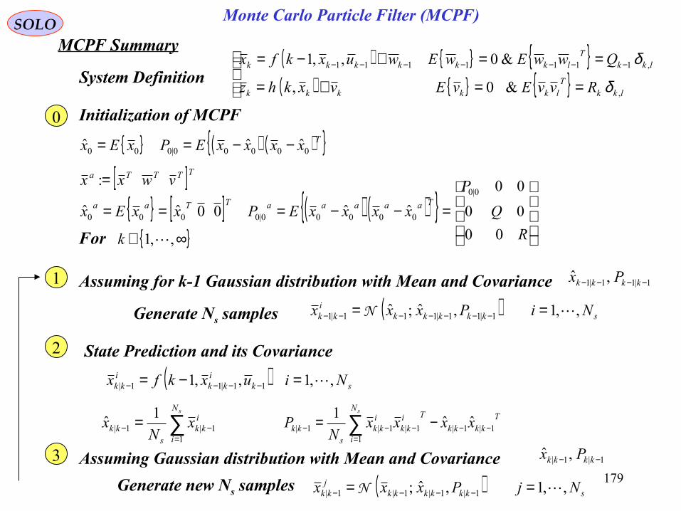
179
Monte Carlo Particle Filter (MCPF)SOLOMCPF Summary
Initialization of MCPF
( ) ( ) TxxxxEPxEx 00000|000 ˆˆˆ −−==
[ ] ( ) ( )
=−−===
R
Q
P
xxxxEPxxExTaaaaaTTaa
00
00
00
ˆˆ00ˆˆ0|0
00000|0000
[ ]TTTTa vwxx =:
For ∞∈ ,,1 k
Assuming for k-1 Gaussian distribution with Mean and Covariance
( ) skkkkki
kk NiPxxx ,,1,ˆ;ˆ 1|11|111|1 == −−−−−−− N
State Prediction and its Covariance
System Definition( ) ( )
==+=
==+−= −−−−−−−
lkkTlkkkkk
lkkT
lkkkkkk
RvvEvEvxkhz
QwwEwEwuxkfx
,
,1111111
&0,
&0,,1
δ
δ
( ) ski
kkikk Niuxkfx ,,1,,1 11|11| =−= −−−−
∑=
−− =sN
i
ikk
skk x
Nx
11|1|
1ˆ
0
1
2
Tkkkk
N
i
Tikk
ikk
skk xxxx
NP
s
1|1|1
1|1|1| ˆˆ1
−−=
−−− −= ∑
1|11|1 ,ˆ −−−− kkkk Px
Generate Ns samples
Assuming Gaussian distribution with Mean and Covariance
( ) skkkkkkjkk NjPxxx ,,1,ˆ; 1|1|1|1| == −−−− N
3 1|1| ,ˆ −− kkkk Px
Generate new Ns samples

180
Monte Carlo Particle Filter (MCPF)SOLOMCPF Summary (continue – 1)
Measure Prediction
( ) sjkk
jkk Njxkhz ,,1, 1|1| == −− ∑
=−− =
sN
j
jkk
skk z
Nz
11|1|
1ˆ
4
Innovation and its Covariance
6
1|ˆ −−= kkkk zzi
( ) ( )∑=
−−−−− −−==sN
j
T
kkjkkkk
jkk
s
zzkkk zzzz
NPS
11|1|1|1|1| ˆˆ
1
Kalman Gain Computations
7
( ) ( )∑=
−−−−− −−=sN
j
T
kkjkkkk
jkk
s
xzkk zzxx
NP
11|1|1|1|1| ˆˆ
1
1
1|1|
−−−= zz
kkxzkkk PPK
Kalman Filter8kkkk
xkk iKx += −1|| ˆµ T
kkkkkxxkk KSKP −=Σ −1||
k := k+1 & return to 1
Predicted Covariances Computations5
Importance Sampling using Gaussian Mean and Covariance
( ) sxxkk
xkkk
mkk Nmxx ,,1,; ||| =Σ= µN
9 xxkk
xkk 1|1| , −− Σµ
Generate new Ns samples
Weight Update10 ( ) ( )( ) sxx
kkxkk
mkk
kkkkmkk
mkkkm
k Nmx
Pxxxzpw ,,1
,;
,ˆ;|~
1|1||
1|1||| =Σ
=−−
−−
µN
Ns
N
l
lk
mk
mk Nmwww
s
,,1~/~1
== ∑=
Update State and its Covariance11 ∑=
=sN
m
mkk
mk
skk xw
Nx
1||
1ˆ ( ) ( )∑
=
−−=sN
m
T
kkmkkkk
mkk
skk xxxx
NP
1||||| ˆˆ
1

181
Sensor DataProcessing andMeasurement
Formation
Observation -to - Track
Association
InputData Track Maintenance
( Initialization,Confirmationand Deletion)
Filtering andPrediction
GatingComputations
Samuel S. Blackman, " Multiple-Target Tracking with Radar Applications", Artech House,1986
Samuel S. Blackman, Robert Popoli, " Design and Analysis of Modern Tracking Systems",Artech House, 1999
SOLO Monte Carlo Particle Filter (MCPF)
Table of Content

182
Estimators
vxHz +=
SOLO
Maximum Likelihood Estimate (MLE)
For the particular vector measurement equation
where the measurement noise, is gaussian (normal), with zero mean:
v
H zx
( )RNv ,0~
( ) ( )( )xp
zxpxzp
x
zxxz
,| ,
| =
and independent of , the conditional probability can be written, using Bayes rule as:
x ( )xzp xz ||
( )
−
−
==−=
1
111
1111
1
1
,
nxpp
nx
pxnxpxnpxpx
xHz
xHz
zxfxHzv
xn
xn
( ) ( ) 2/1
,, /,, T
vxzx JJvxpzxp =
The measurement noise can be related to and by the function:v zx
pxp
p
pp
p
I
z
f
z
f
z
f
z
f
z
fJ =
∂∂
∂∂
∂∂
∂∂
=
∂∂=
1
1
1
1
( ) ( ) ( ) ( )vpxpvxpzxp vxvxzx ⋅== ,, ,,
v
Since the measurement noise is independent of :xv
zThe joint probability of and is given by:x
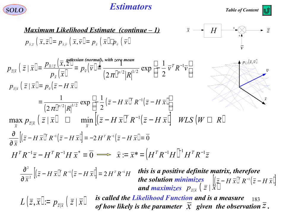
183
EstimatorsSOLO
Maximum Likelihood Estimate (continue – 1)
v
H zx
( ) ( ) ( ) ( )vpxpvxpzxp vxvxzx ⋅== ,, ,,
x
v
( )vxp vx ,,
( ) ( )
( )( ) ( )
−−−=
−=
− xHzRxHzR
xHzpxzp
T
p
vxz
12/12/
|
2
1exp
2
1
|
π
( ) ( ) ( )[ ] ( )RWWLSxHzRxHzxzp T
xxz
x⇒−−⇔ −1
| min|max
( ) ( )[ ] ( ) 02 11 =−−=−−∂∂ −− xHzRHxHzRxHzx
TT
0*11 =− −− xHRHzRH TT ( ) zRHHRHxx TT 111*: −−−==
( ) ( )[ ] HRHxHzRxHzx
TT 11
2
2
2 −− =−−∂∂ this is a positive definite matrix, therefore
the solution minimizesand maximizes
( ) ( )[ ]xHzRxHz T −− −1
( )xzp xz ||
( ) ( )( ) ( )
( )
−=== − vRv
Rvp
xp
zxpxzp T
pvx
zxxz
12/12/
/| 2
1exp
2
1,|
π
gaussian (normal), with zero mean
( ) ( )xzpxzL xz |:, |= is called the Likelihood Function and is a measureof how likely is the parameter given the observation .x z
Table of Content

184
EstimatorsSOLO
Bayesian Maximum Likelihood Estimate (Maximum Aposteriori– MAP Estimate)
v
H zxvxHz +=Consider a gaussian vector , where ,measurement, , where the gaussian noiseis independent of and .( )RNv ,0~
vx ( ) ( )[ ]−− PxNx ,~
x
( )( ) ( )
( )( ) ( ) ( )( )
−−−−−−
−= − xxPxx
Pxp T
nx
1
2/12/ 2
1exp
2
1
π
( ) ( )( )
( ) ( )
−−−=−= − xHzRxHz
RxHzpxzp T
pvxz1
2/12/| 2
1exp
2
1|
π
( ) ( ) ( ) ( )∫∫+∞
∞−
+∞
∞−
== xdxpxzpxdzxpzp xxzzxz |, |,
is gaussian with( )zp z ( ) ( ) ( ) ( ) ( )−=+=+= xHvExEHvxHEzE
0
( ) ( )[ ] ( )[ ] ( )[ ] ( )[ ] ( )( )[ ] ( )( )[ ] ( )[ ] ( )[ ] ( )[ ] ( )[ ] ( ) RHPHvvEHxxvEvxxEH
HxxxxEHvxxHvxxHE
xHvxHxHvxHEzEzzEzEz
TTTTT
TTT
TT
+−=+−−−−−−
−−−−=+−−+−−=
−−+−−+=−−=
00
cov
( )( ) ( )
( )[ ] ( )[ ] ( )[ ]
−−+−−−−
+−= −
xHzRHPHxHzRHPH
zp TT
Tpz ˆˆ2
1exp
2
1 1
2/12/π

185
EstimatorsSOLO
Bayesian Maximum Likelihood Estimate (Maximum Aposteriori Estimate) (continue – 1)
v
H zxvxHz +=Consider a gaussian vector , where ,measurement, , where the gaussian noiseis independent of and .( )RNv ,0~
vx ( ) ( )[ ]−− PxNx ,~
x
( )( ) ( )
( )( ) ( ) ( )( )
−−−−−−
−= − xxPxx
Pxp T
nx
1
2/12/ 2
1exp
2
1
π
( ) ( )( )
( ) ( )
−−−=−= − xHzRxHz
RxHzpxzp T
pvxz1
2/12/| 2
1exp
2
1|
π
( )( ) ( )
( )[ ] ( )[ ] ( )[ ]
−−+−−−−
+−= −
xHzRHPHxHzRHPH
zp TT
Tpz ˆˆ2
1exp
2
1 1
2/12/π
( ) ( ) ( )( ) ( ) ( )
( )
( ) ( ) ( )( ) ( ) ( )( ) ( )[ ] ( )[ ] ( )[ ]
−−+−−−+−−−−−−−−−⋅
+−
−==
−−− xHzRHPHxHzxxPxxxHzRxHz
RHPH
RPzp
xpxzpzxp
TTTT
T
nz
xxzzx
ˆˆ2
1
2
1
2
1exp
2
1||
111
2/1
2/12/12/
||
π
from which
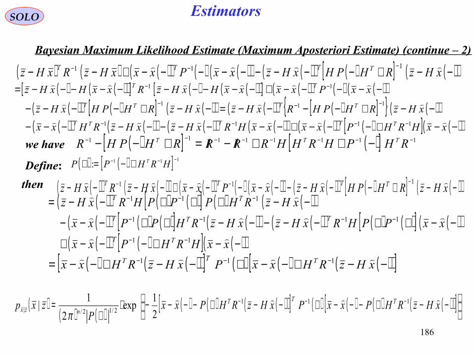
186
EstimatorsSOLO
Bayesian Maximum Likelihood Estimate (Maximum Aposteriori Estimate) (continue – 2)
( ) ( ) ( )( ) ( ) ( )( ) ( )( ) ( )[ ] ( )( )−−+−−−−−−−−−+−−−−− xHzRHPHxHzxxPxxxHzRxHz TTTT 111
( ) ( )( )[ ] ( ) ( )( )[ ] ( )( ) ( ) ( )( )( )( ) ( )[ ] ( )( ) ( )( ) ( )[ ] ( )( )
( )( ) ( )( ) ( )( ) ( )( ) ( )( ) ( )[ ] ( )( )−−+−−−+−−−−−−−−−−
−−+−−−−=−−+−−−−
−−−−−+−−−−−−−−−−=
−−−−
−−−
−−
xxHRHPxxxxHRxHzxHzRHxx
xHzRHPHRxHzxHzRHPHxHz
xxPxxxxHxHzRxxHxHz
TTTTT
TTTT
TT
1111
111
11
( )( ) ( )( ) ( )( ) ( ) ( )( ) ( )( ) ( )[ ] ( )( )−−+−−−−−−−−−+−−−−−−− xHzRHPHxHzxxPxxxHzRxHz TTTT 111
( )[ ] ( )[ ] 11111111 −−−−−−−− −++/−/=+−− RHPHRHHRRRRHPHR TTTwe have
then
Define: ( ) ( )[ ] 111:−−− +−=+ HRHPP T
( )( ) ( ) ( )[ ] ( ) ( )( )( )( ) ( ) ( )[ ] ( )( ) ( )( ) ( ) ( )[ ] ( )( )( )( ) ( )[ ] ( )( )−−+−−−+
−−++−−−−−++−−−
−−+++−−=
−−
−−−−
−−−
xxHRHPxx
xxPPHRxHzxHzRHPPxx
xHzRHPPPHRxHz
TT
TTT
TT
11
1111
111
( ) ( )( )[ ] ( ) ( ) ( )( )[ ]−−+−−+−−+−−= −−− xHzRHxxPxHzRHxx TTT 111
( )( ) ( )
( ) ( ) ( )( )[ ] ( ) ( ) ( ) ( )( )[ ]
−−+−−−+−−+−−−−⋅
+= −−− xHzRHPxxPxHzRHPxx
Pzxp TTT
nzx
1112/12/| 2
1exp
2
1|
π
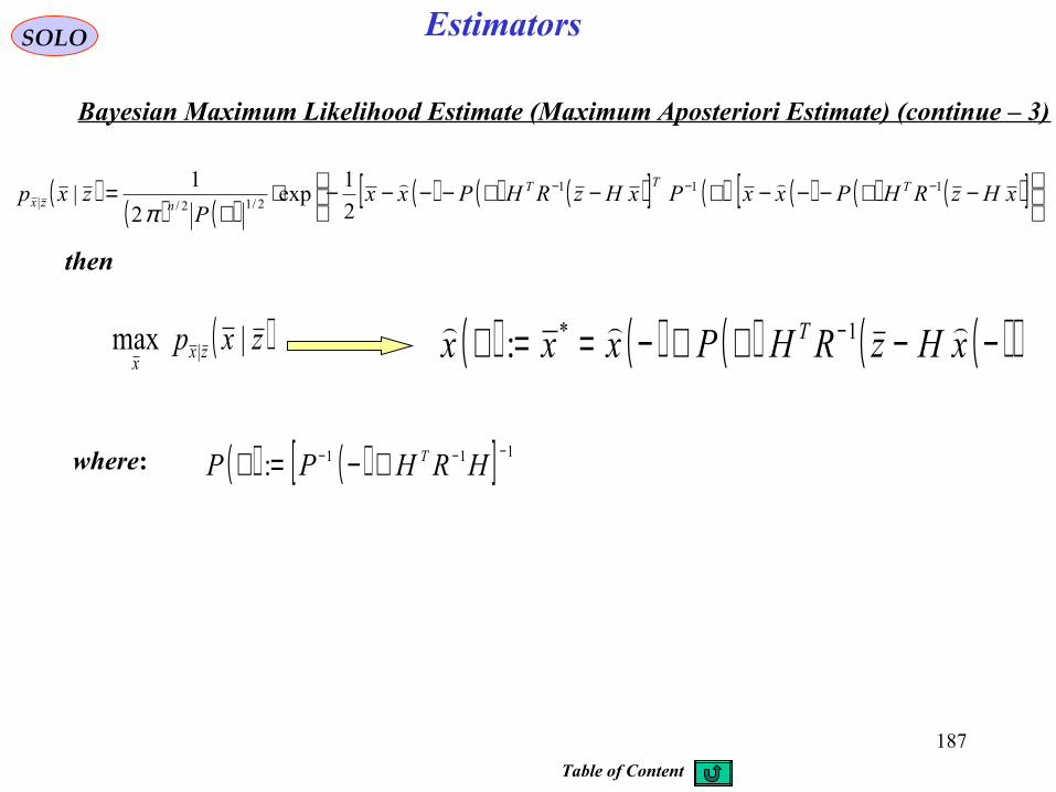
187
EstimatorsSOLO
Bayesian Maximum Likelihood Estimate (Maximum Aposteriori Estimate) (continue – 3)
then
where: ( ) ( )[ ] 111:−−− +−=+ HRHPP T
( )( ) ( )
( ) ( ) ( )[ ] ( ) ( ) ( ) ( )[ ]
−+−−−+−+−−−−⋅
+= −−− xHzRHPxxPxHzRHPxx
Pzxp TTT
nzx111
2/12/| 2
1exp
2
1|
π
( )zxp zxx
|max | ( ) ( ) ( ) ( )( )−−++−==+ − xHzRHPxxx T 1*:
Table of Content

SOLO
( ) ( ) ( ) [ ]fttttwddttxftxd ,, 0∈+=A continuous dynamic system is described by:
Nonlinear Filters
( )tx - n- dimensional state vector
( )twd - n- dimensional process noise vector described by the covariance matrix Q
- the probability of the state at time tx
The time evolution of the probability density function is described by the Fokker–Planck equation:
Nonlinear Filters based on the Fokker-Planck Equation
Fred Daum from Raytheon Company leads methods to design NonlinearFilters starting from Fokker-Planck Equation.
( ) ( ) 0:ˆ == twdEtwd
( ) ( )[ ] ( ) ( )[ ] ( ) ( )τδ −=−− ttQtwdtwdtwdtwdE Tˆˆ
Return to StochasticProcesses
( ) ( )[ ] ( )[ ] ( ) ( )[ ]( ) ( ) ( ) ( )[ ]
∂
∂∂∂+
∂∂
−=∂
∂x
txptQ
xx
txpttxf
t
txp txtxtx
2
1,
( )[ ]txp
Fred Daum
( )[ ] ( ) ( )[ ]( ) ( )[ ] ( ) ( )[ ]( )∑ = ∂
∂=
∂∂ n
ii
txitx
x
txpttxf
x
txpttxf1
,,( ) ( )[ ] ( ) ( )[ ] ( ) ( )[ ] ( ) ( )[ ] T
n
txtxtxtx
x
txp
x
txp
x
txp
x
txp
∂
∂∂
∂∂
∂=
∂∂
,,,21
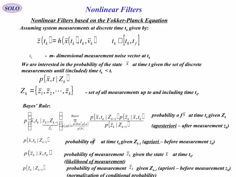
SOLO
Assuming system measurements at discrete time tk given by:
( ) ( )( ) [ ]fkkkkk tttvttxhtz ,,, 0∈=
kv - m- dimensional measurement noise vector at tk
We are interested in the probability of the state at time t given the set of discrete measurements until (included) time tk < t.
x
( )kZtxp |,
kk zzzZ ,,, 21 = - set of all measurements up to and including time tk.
Bayes’ Rule:
Nonlinear Filters
( ) ( ) ( )( )
( ) ( )( )1
1
||
1 |
,||,,|,
−
−
=− =
kk
kkkkBayes
bp
apabpbap
Z
kkk Zzp
txzpZtxpZztxp
k
( )1|, −kk Ztxp probability of at time tk given Zk-1 (apriori – before measurement zk)x
(aposteriori – after measurement zk)
probability o f at time tk given Zk x
( )kk txzp ,| probability of measurement given the state at time tk. (likelihood of measurement)
kz x
( )1| −kk Zzp probability of measurement given Zk-1 (apriori – before measurement zk)(normalization of conditional probability)
kz
Nonlinear Filters based on the Fokker-Planck Equation

SOLO
In the Classical Particle Filter solution the particle are drawn using the apriori density that decide their distribution (see Figure). After measurement the Likelihood ofMeasurement is obtained and nothingwill prevent a low density of particlesdrawn before in the Likelihood region.This is the Particle Degeneracy, thatproduce the curse of dimensionality.
Nonlinear Filters
Fred Daum
Nonlinear Filters based on the Fokker-Planck Equation
prior density
Particles to represent prior density
Liklehood of measurement
Particle DegeneracyCause of Curse of Dimensionality
The Particle Filter solutions have implementations problems.
The Number of Particles necessary to reduce the Filter Error increase with System Dimension. Daum gives the Filter Error as function of Number of Particles for System Dimension as Parameter.
http://sc.enseeiht.fr/doc/Seminar_Daum_2012_2.pdf

SOLO
By taking natural logarithm of the conditional probability, we get in the right side a sum of logarithms
Nonlinear Filters
Fred Daum( ) ( ) ( ) ( )
ionnormalizat
kk
likelihood
kk
aprior
kk
aposterior
kk ZzptxzpZtxpZtxp 11 |ln,|ln|,ln|,ln −− −+=
The homotopy
( ) ( ) ( ) ( )
ionnormalizatlikelihoodaprioraposterior
Kxhxgxp λλλ lnlnln,ln −+=p.d.f.
p.d.f.Flow of Density
particles particles
Flow of Particles
Sample from Density
Sample from Density
aprioriaposteriori
Induced Flow of Particles for Bayes¶Rule
Since p (x,λ) is the p.d.f. associated to a system defined by f (x,λ) we have the Fokker-Plank Equation:
( ) ( ) ( )( ) ( ) ( )
∂
∂∂∂+
∂∂−=
∂∂
x
xpxQ
xx
xpxfxp λλλλλ
λ ,,
2
1,,,
To obtain the aposteriori probability p (x,tk|Zk) from the apriori probability p (x,tk|Zk-1) and the likelihood p (zk|x,tk), Daum uses a homotopy procedure (see next slide) by choosing a homotopy continuous parameter λ ϵ [0,1]. He will search for a function (not related to the filtered system) that describes the flow of the particles and is associated to p (x,tk|Zk) .
( )λ,xf
Nonlinear Filters based on the Fokker-Planck Equation
( )λ,xQ - Noise Spectrum to be defined
Here we describe Daum proposed methods called Particle Flow Filters
( ) ( )λ
λλλ d
wdxQxf
d
xd,, += Particle Flow Equation

01/13/15 192
HomotopyIn topology, two continuous functions from one topological space to another are called homotopic (Greek μός (homós) = same, similarὁ , and τόπος (tópos) = place) if one can be "continuously deformed" into the other, such a deformation being called a homotopy between the two functions. An outstanding use of homotopy is the definition of homotopy groups and cohomotopy groups, important invariants in algebraic topology.
A Homotopy of a Coffe Cup into a doughnut
Formally, a homotopy between two continuous functions f and g from a topological space X to a topological space Y is defined to be a continuous function H : X × [0,1] → Y from the product of the space X with the unit interval [0,1] to Y such that, if x X then H(x,0) = f(x) and H(x,1) = ∈g(x).If we think of the second parameter of H as time then H describes a continuous deformation of f into g: at time 0 we have the function f and at time 1 we have the function g.An alternative notation is to say that a homotopy between two continuous functions f, g : X → Y is a family of continuous functions ht : X → Y for t ∈ [0,1] such that h0 = f and h1 = g, and the map t h↦ t is continuous from [0,1] to the space of all continuous functions X → Y. The two versions coincide by setting ht(x) = H(x,t).
Formal definition
SOLO
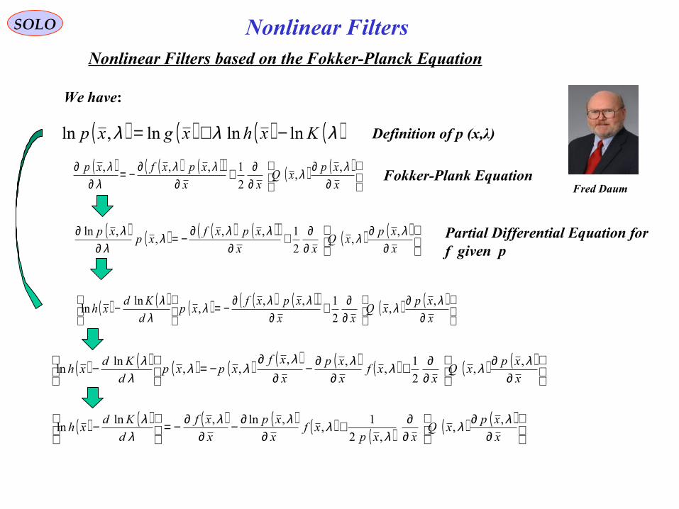
SOLO Nonlinear Filters
Fred Daum
( ) ( ) ( )( ) ( ) ( )
∂
∂∂∂+
∂∂−=
∂∂
x
xpxQ
xx
xpxfxp λλλλλ
λ ,,
2
1,,,Fokker-Plank Equation
( ) ( ) ( ) ( ) ( )( ) ( ) ( )
∂
∂∂∂+
∂∂−=
−
x
xpxQ
xx
xpxfxp
d
Kdxh
λλλλλλ
λ ,,
2
1,,,
lnln
Partial Differential Equation for f given p
( ) ( ) ( ) ( )( ) ( ) ( )
∂
∂∂∂+
∂∂−=
∂∂
x
xpxQ
xx
xpxfxp
xp λλλλλλ
λ ,,
2
1,,,
,ln
( ) ( ) ( ) ( )λλλ Kxhxgxp lnlnln,ln −+= Definition of p (x,λ)
We have:
( ) ( ) ( ) ( ) ( ) ( ) ( ) ( ) ( )
∂
∂∂∂+
∂∂−
∂∂
−=
−
x
xpxQ
xxf
x
xp
x
xfxpxp
d
Kdxh
λλλλλλλ
λλ ,
,2
1,
,,,,
lnln
( ) ( ) ( ) ( ) ( ) ( ) ( ) ( )
∂
∂∂∂+
∂∂−
∂∂−=
−
x
xpxQ
xxpxf
x
xp
x
xf
d
Kdxh
λλλ
λλλλ
λ ,,
,2
1,
,ln,lnln
Nonlinear Filters based on the Fokker-Planck Equation

SOLO Nonlinear Filters
Fred Daum
( ) ( ) ( ) ( ) ( ) ( ) ( ) ( )
∂
∂∂∂+
∂∂−
∂∂−=
−
x
xpxQ
xxpxf
x
xp
x
xf
d
Kdxh
λλλ
λλλλ
λ ,,
,2
1,
,ln,lnln
Differentiate this Equation as function of x
( ) ( ) ( ) ( ) ( ) ( ) ( ) ( ) ( )
∂
∂∂∂
∂∂+
∂∂∂−
∂
∂∂∂−
∂∂−=
∂∂ λλλλλλλλ ,/
,,
2
1,,ln,,ln,
ln2
2
xpx
xpxQ
xxx
xf
x
xp
x
xf
xx
xpxf
x
xh T
One option to simplify the problem is to choose such that:( )λ,xQ
( ) ( ) ( ) ( ) ( ) ( ) 0,/,
,2
1,,ln, =
∂
∂∂∂
∂∂+
∂∂∂−
∂
∂∂∂− λλλλλλ
xpx
xpxQ
xxx
xf
x
xp
x
xf
x
We obtain ( ) ( ) ( )2
2 ,ln,
ln
x
xpxf
x
xh T
∂∂−=
∂∂ λλ ( ) ( ) ( ) T
x
xh
x
xpxf
∂
∂
∂
∂−=−
ln,ln,
1
2
2 λλ
Nonlinear Filters based on the Fokker-Planck Equation
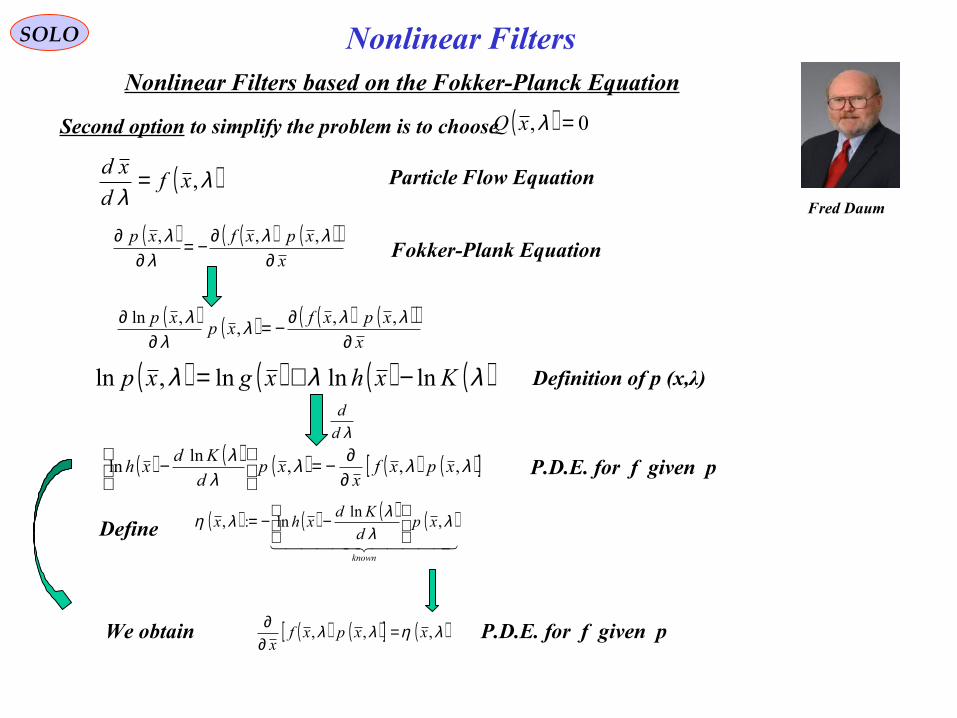
SOLO Nonlinear Filters
Fred Daum
Second option to simplify the problem is to choose ( ) 0, =λxQ
Nonlinear Filters based on the Fokker-Planck Equation
( )λλ
,xfd
xd =
( ) ( ) ( )( )x
xpxfxp
∂∂−=
∂∂ λλ
λλ ,,,
Fokker-Plank Equation
Particle Flow Equation
( ) ( ) ( ) ( )λλλ Kxhxgxp lnlnln,ln −+= Definition of p (x,λ)
Define ( ) ( ) ( ) ( )
known
xpd
Kdxhx λ
λλλη ,
lnln:,
−−=
We obtain ( ) ( )[ ] ( )ληλλ ,,, xxpxfx
=∂∂ P.D.E. for f given p
( ) ( ) ( ) ( )( )x
xpxfxp
xp
∂∂−=
∂∂ λλλ
λλ ,,
,,ln
( ) ( ) ( ) ( ) ( )[ ]λλλλ
λ,,,
lnln xpxf
xxp
d
Kdxh
∂∂−=
− P.D.E. for f given p
λdd

SOLO Nonlinear Filters
Fred Daum
Second option to simplify the problem is to choose ( ) 0, =λxQ
Nonlinear Filters based on the Fokker-Planck Equation
We obtain ( ) ( )[ ]( )
( )ληλλλ
,,,,
xxpxfx
xq
=∂∂
q = p ff = unknown functionp & η known at random points( ) ( ) ( ) ( )λ
λλλη ,
lnln:, xp
d
Kdxhx
−−=
We have ( )λη ,2
2
1
1 xx
q
x
q
x
q
x
q
d
d =∂∂++
∂∂+
∂∂=
∂∂
1. Linear PDE in unknown f or q.2. Constant coefficient PDE in q.3. First Order PDE.4. Highly undetermined PDE.5. Same as the Gauss divergence law in Maxwell Equations.6. Same as Euler’s Equation in Fluid Dynamics.7. Existence of solutions if and only if integral of η is zero.
Exact Flow Solutions for g & h Gaussian Densities:( ) ( ) ( )( ) [ ]
( ) ( ) ( )[ ]xAzRHPAIAIb
HRHPHHPA
bxAxf
T
TT
+++=
+−=
+=
−
−
1
1
2:
2
1:
,
λλλ
λλ
λλλ Automatically stable under very mild conditions & extremely fast

Fred Daum
SOLO Nonlinear Filters
F. Daum, J. Huang, Particle Flow for Nonlinear Filters, Bayesian Decision and Transport, 7 April 2014
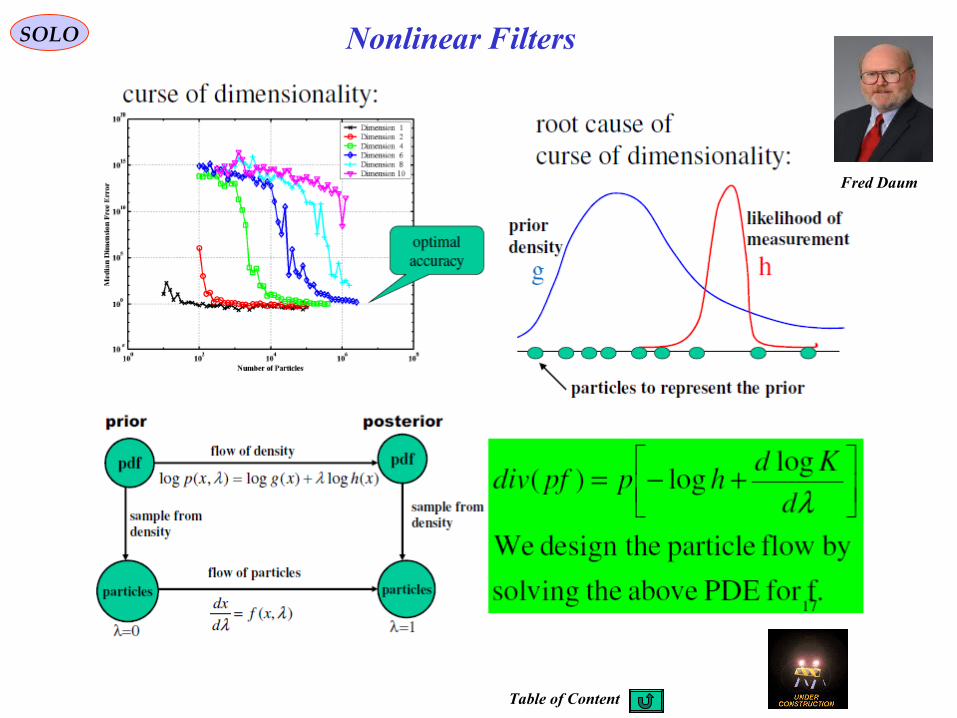
SOLO Nonlinear Filters
Fred Daum
Table of Content

199
Recursive Bayesian Estimation
References:
SOLO
1. Sage, A.P., & Melsa, J.L., “Estimation Theory with Applications to Communications and Control”, McGraw Hill, 19712. Gordon, N.J., Salmond, D.J., Smith, A.M.F., “Novel Approach to
Nonlinear/Non- Gaussian Bayesian State Estimation”, IEE Proceedings Radar and Signal Processing, vol. 140, No. 2, April 1993, pp. 107 - 113
7. Haug, A.J., “A Tutorial on Bayesian Estimation and Tracking Techniques Applicable to Nonlinear and Non-Gaussian Processes”, MITRE Corporation,
January 2005
5. Arulampalam,S., Maskell,S., Gordon,N., Clapp,T., “A Tutorial on Particle Filters for On-line Non-linear/Non-Gaussian Bayesian Tracking”, IEEE
Transactions on Signal Processing, Vol. 50, No. 2, February 2002
6. Ristic,B., Arulampalam,S., Gordon,N., “Beyond the Kalman Filter Particle Filters for Tracking Applications”, Artech House, 2004
4. Karlsson, R., “Simulation Based Methods for Target Tracking”, Department of Electrical Engineering Linköpings Universitet, 2002
3. Doucet,A., de Freitas,N., Gordon,N., Ed. “Sequential Monte Carlo Methods in Practice”, Springer, 2001
200
Recursive Bayesian Estimation
References (continue – 1):
SOLO
Fred Daum, “Particle Flow for Nonlinear Filters”, 19 July 2012
http://sc.enseeiht.fr/doc/Seminar_Daum_2012_2.pdf
https://www.ll.mit.edu/asap/asap_06/pdf/Papers/23_Daum_Pa.pdf
Fred Daum, Misha Krichman, “Non-Particle Filters”,
F. Daum, J. Huang, Particle Flow for Nonlinear Filters, Bayesian Decision and Transport, 7 April 2014
http://meeting.xidian.edu.cn/workshop/miis2014/uploads/files/July-5th-930am_Fred%20Daum_Particle%20flow%20for%20nonliner%20filters,%20Bayesuan%20Decisions%20and%20Transport%20.pdf
http://www.dsi.unifi.it/users/chisci/idfric/Nonlinear_filtering_Chen.pdf
Zhe Chen, “Bayesian Filtering From Kalman Filters to Particle Filters, and Beyond”, 18.05.06,
Table of Content

201January 13, 2015 201
SOLO
TechnionIsraeli Institute of Technology
1964 – 1968 BSc EE1968 – 1971 MSc EE
Israeli Air Force1970 – 1974
RAFAELIsraeli Armament Development Authority
1974 – 2013
Stanford University1983 – 1986 PhD AA
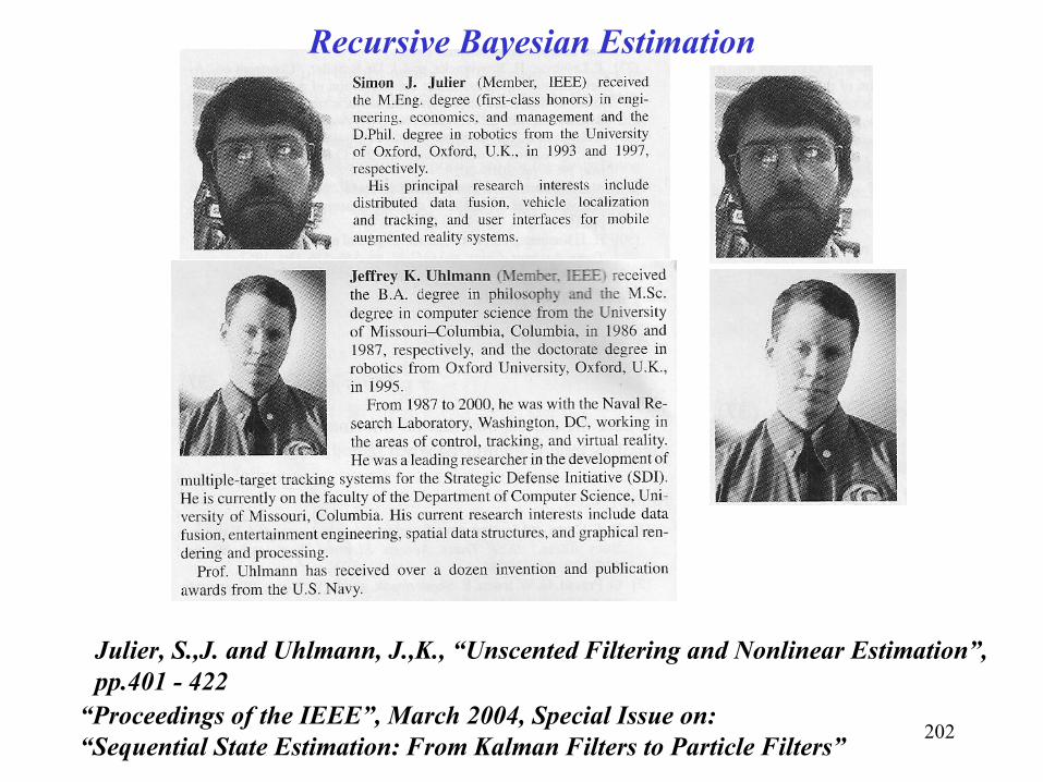
202“Proceedings of the IEEE”, March 2004, Special Issue on:“Sequential State Estimation: From Kalman Filters to Particle Filters”
Julier, S.,J. and Uhlmann, J.,K., “Unscented Filtering and Nonlinear Estimation”,pp.401 - 422
Recursive Bayesian Estimation

203
SOLO
Neil GordonM. Sanjev Arulampalam
Tim ClappSimon MaskellNando de FreitasArnaud Doucet
Branko Ristic
Genshiro Kitagawa Christophe Andrieu
Dan Crişan Fred Daum
Recursive Bayesian Estimation

204
Markov Chain Monte Carlo (MCMC)SOLO
Some MCMC Developments Related to Vision
Nicholas Constantine Metropolis ( 1915 – 1999)
Metropolis 1946
Hastings 1970
Heat bath
Miller, Grenader, 1994
Green 1995
DDMCMC 2001 - 2005
Waltz 1972, (labeling)
Rosenfeld, Hummel, Zucker 1976 (relaxation)
Geman brothers 1984, (Gibbs sampler)
Kirkpatrick 1983
Swendsen-Wang 1987(clustering)
Swendsen-Wang Cut 2003

205
Markov Chain Monte Carlo (MCMC)SOLO
A Brief History of MCMC
Nicholas Constantine Metropolis ( 1915 – 1999)
1942 – 1946: Real use of Monte Carlo started during WWII- study of the atomic bomb (neutron diffusion in fissile material)
1948: Fermi, Metropolis, Ulam obtained Monte Carlo estimates forthe eigenvalues of the Schrödinger equations.
1950: Formating of the basic construction of MCMC, e.g. the Metropolis method- application to statistical physics model, such as Ising model
1960 - 80: using MCMC to study phase transition; material growth/defect,macro molecules (polymers), etc.
1980s: Gibbs samples (Germ brothers), Simulated annealing, data augmentation, Swendsen-Wang, etc.global optimization; image and spech; quantum field theory
1990s: Applications in genetics; computational biology.
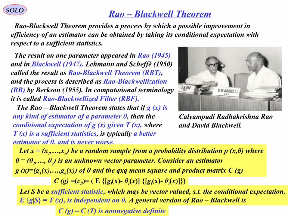
206
Rao – Blackwell TheoremSOLO
Rao-Blackwell Theorem provides a process by which a possible improvement in efficiency of an estimator can be obtained by taking its conditional expectation with respect to a sufficient statistics.
The result on one parameter appeared in Rao (1945) and in Blackwell (1947). Lehmann and Scheffè (1950) called the result as Rao-Blackwell Theorem (RBT), and the process is described as Rao-Blackwellization (RB) by Berkson (1955). In computational terminology it is called Rao-Blackwellized Filter (RBF).
Calyampudi Radhakrishna Rao and David Blackwell.
The Rao – Blackwell Theorem states that if g (x) isany kind of estimator of a parameter θ, then theconditional expectation of g (x) given T (x), whereT (x) is a sufficient statistics, is typically a better estimator of θ, and is never worse. Let x = (x1,…,xn) be a random sample from a probability distribution p (x,θ) whereθ = (θ1,…, θq) is an unknown vector parameter. Consider an estimator g (x)=(g1(x),…,gq(x)) of θ and the qxq mean square and product matrix C (g)
C (g) =(cij)= ( E [gi(x)- θi(x)] [gj(x)- θj(x)])
Let S be a sufficient statistic, which may be vector valued, s.t. the conditional expectation,E g|S = T (x), is independent on θ. A general version of Rao – Blackwell is
C (g) – C (T) is nonnegative definite

207
SOLO Non-Gaussian Distribution Approximation

208
SOLO Non-Gaussian Distribution Approximationhttp://www.dsi.unifi.it/users/chisci/idfric/Nonlinear_filtering_Chen.pdf