3-d plots/symbolic toolboxadonahu1/assets/matlab_class/...mar 06, 2013 · 3-d plots/symbolic...

3-D Plots/Symbolic Toolbox

Aaron S. Donahue

Department of Civil and Environmental Engineering and Earth SciencesUniversity of Notre Dame

March 6, 2013

CE20140

A. S. Donahue (University of Notre Dame) Lecture 13 1 / 21

Outline*

3-D plots

3-D Plotting CommandsManipulating 3-D PlotsIncluding contour values

Making “more attractive” labels and text on plots

Symbolic Toolbox

* This is all extra stuff for lecture, not required for final project.


3-D Plots from last time

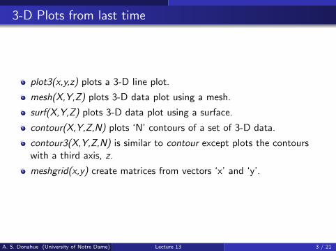
plot3(x,y,z) plots a 3-D line plot.

mesh(X,Y,Z) plots 3-D data plot using a mesh.

surf(X,Y,Z) plots 3-D data plot using a surface.

contour(X,Y,Z,N) plots ‘N’ contours of a set of 3-D data.

contour3(X,Y,Z,N) is similar to contour except plots the contourswith a third axis, z.

meshgrid(x,y) create matrices from vectors ‘x’ and ‘y’.


Manipulating 3-D plots

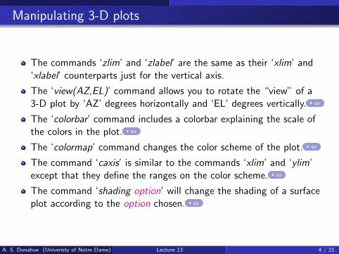
The commands ‘zlim’ and ‘zlabel’ are the same as their ‘xlim’ and‘xlabel’ counterparts just for the vertical axis.

The ‘view(AZ,EL)’ command allows you to rotate the “view” of a3-D plot by ‘AZ’ degrees horizontally and ‘EL’ degrees vertically. ex

The ‘colorbar’ command includes a colorbar explaining the scale ofthe colors in the plot. ex

The ‘colormap’ command changes the color scheme of the plot. ex

The command ‘caxis’ is similar to the commands ‘xlim’ and ‘ylim’except that they define the ranges on the color scheme. ex

The command ‘shading option’ will change the shading of a surfaceplot according to the option chosen. ex


Including Contour information on Contour Plots

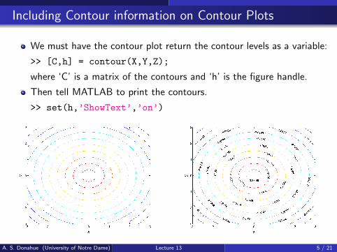
We must have the contour plot return the contour levels as a variable:

>> [C,h] = contour(X,Y,Z);

where ‘C’ is a matrix of the contours and ‘h’ is the figure handle.

Then tell MATLAB to print the contours.

>> set(h,’ShowText’,’on’)


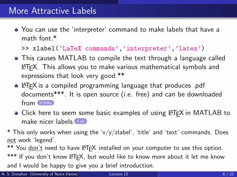
More Attractive Labels

You can use the ‘interpreter’ command to make labels that have amath font.*

>> xlabel(’LaTeX commands’,’interpreter’,’latex’)

This causes MATLAB to compile the text through a language calledLATEX. This allows you to make various mathematical symbols andexpressions that look very good.**

LATEX is a compiled programming language that produces .pdfdocuments***. It is open source (i.e. free) and can be downloadedfrom links

Click here to seem some basic examples of using LATEX in MATLAB tomake nicer labels. ex

* This only works when using the ‘x/y/zlabel’, ‘title’ and ‘text’ commands. Doesnot work ‘legend’.** You don’t need to have LATEX installed on your computer to use this option.

*** If you don’t know LATEX, but would like to know more about it let me know

and I would be happy to give you a brief introduction.A. S. Donahue (University of Notre Dame) Lecture 13 6 / 21

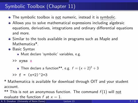
Symbolic Toolbox (Chapter 11)

The symbolic toolbox is not numeric, instead it is symbolic.

Allows you to solve mathematical expressions including algebraicequations, derivatives, integrations and ordinary differential equationsand more.

Similar to the tools available in programs such as Maple andMathematica*.Basic Syntax

Must declare ‘symbolic’ variables, e.g.

>> syms x

Then declare a function**, e.g. f = (x + 2)2 + 3

>> f = (x+2)^2+3

* Mathematica is available for download through OIT and your studentaccount.** This is not an anonymous function. The command f (1) will notevaluate the function f at x = 1.


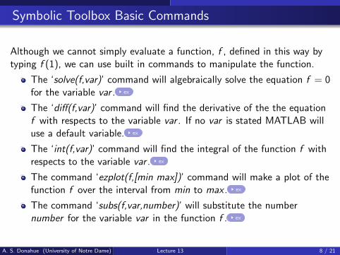
Symbolic Toolbox Basic Commands

Although we cannot simply evaluate a function, f , defined in this way bytyping f (1), we can use built in commands to manipulate the function.

The ‘solve(f,var)’ command will algebraically solve the equation f = 0for the variable var . ex

The ‘diff(f,var)’ command will find the derivative of the the equationf with respects to the variable var . If no var is stated MATLAB willuse a default variable. ex

The ‘int(f,var)’ command will find the integral of the function f withrespects to the variable var . ex

The command ‘ezplot(f,[min max])’ command will make a plot of thefunction f over the interval from min to max . ex

The command ‘subs(f,var,number)’ will substitute the numbernumber for the variable var in the function f . ex


Thank you

This finishes the MATLAB portion of the Methods of Engineering IIcourse.

Thank you all for a wonderful half–semester and I wish you luck inAutoCad.

Its been a pleasure teaching you!


The Following Slides provide examples of the topicscovered in this lecture.


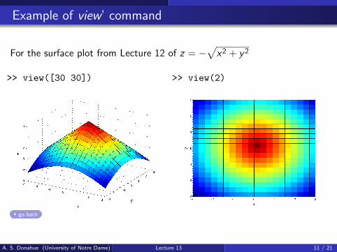
Example of view’ command

For the surface plot from Lecture 12 of z = −√

x2 + y2

>> view([30 30]) >> view(2)

go back


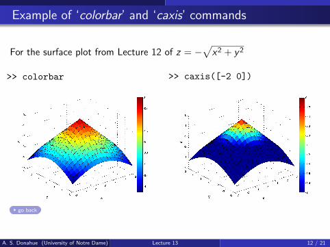
Example of ‘colorbar’ and ‘caxis’ commands


x2 + y2

>> colorbar >> caxis([-2 0])

go back


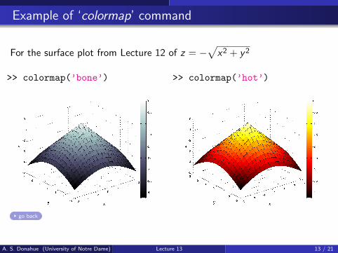
Example of ‘colormap’ command


x2 + y2

>> colormap(’bone’) >> colormap(’hot’)

go back


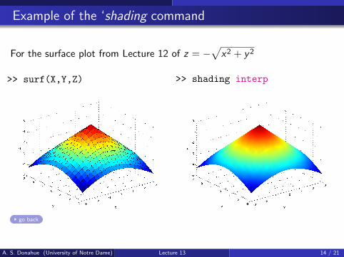
Example of the ‘shading command


x2 + y2

>> surf(X,Y,Z) >> shading interp

go back


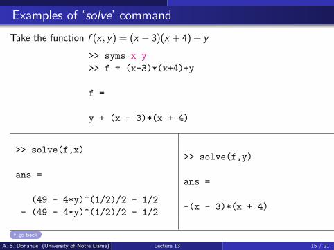
Examples of ‘solve’ command

Take the function f (x , y) = (x − 3)(x + 4) + y

>> syms x y

>> f = (x-3)*(x+4)+y

f =

y + (x - 3)*(x + 4)

>> solve(f,x)

ans =

(49 - 4*y)^(1/2)/2 - 1/2

- (49 - 4*y)^(1/2)/2 - 1/2

>> solve(f,y)

ans =

-(x - 3)*(x + 4)

go back


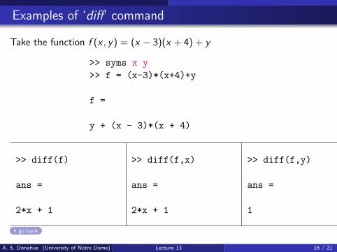
Examples of ‘diff’ command

Take the function f (x , y) = (x − 3)(x + 4) + y

>> syms x y

>> f = (x-3)*(x+4)+y

f =

y + (x - 3)*(x + 4)

>> diff(f)

ans =

2*x + 1

>> diff(f,x)

ans =

2*x + 1

>> diff(f,y)

ans =

1

go back


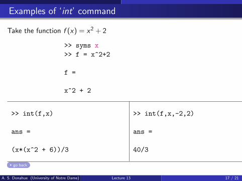
Examples of ‘int’ command

Take the function f (x) = x2 + 2

>> syms x

>> f = x^2+2

f =

x^2 + 2

>> int(f,x)

ans =

(x*(x^2 + 6))/3

>> int(f,x,-2,2)

ans =

40/3

go back


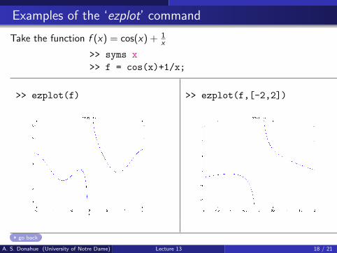
Examples of the ‘ezplot’ command

Take the function f (x) = cos(x) + 1x

>> syms x

>> f = cos(x)+1/x;

>> ezplot(f) >> ezplot(f,[-2,2])

go back


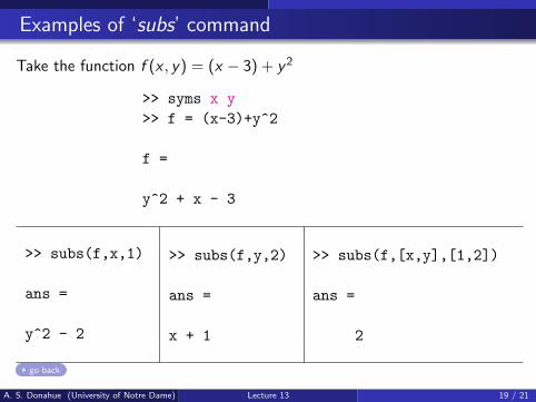
Examples of ‘subs’ command

Take the function f (x , y) = (x − 3) + y2

>> syms x y

>> f = (x-3)+y^2

f =

y^2 + x - 3

>> subs(f,x,1)

ans =

y^2 - 2

>> subs(f,y,2)

ans =

x + 1

>> subs(f,[x,y],[1,2])

ans =

2

go back


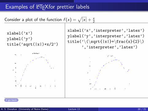
Examples of LATEXfor prettier labels

Consider a plot of the function f (x) =√|x |+ x

2

xlabel(’x’)

ylabel(’y’)

title(’sqrt(|x|)+x/2’)

xlabel(’x’,’interpreter’,’latex’)

ylabel(’y’,’interpreter’,’latex’)

title(’\(\sqrt{|x|}+\frac{x}{2}\)’,’interpreter’,’latex’)

go back


LATEX links

The following links are for programs that will assist you in running LATEXonyour system.

You first need the source code. Information for getting the sourcecode for any platform can be found at:

http://latex-project.org/ftp.html link

You may also want to download a program to help you compileLATEXand generate LATEXdocuments.

http://pages.uoregon.edu/koch/texshop/obtaining.html link

http://www.texniccenter.org/ link

http://en.wikipedia.org/wiki/Comparison of TeX editors link

Lastly an amazing source of information for all things LATEXis thewikibook which can be found at the link

http://en.wikibooks.org/wiki/LaTeX link

go back


http://latex-project.org/ftp.html

http://pages.uoregon.edu/koch/texshop/obtaining.html

http://www.texniccenter.org/

http://en.wikipedia.org/wiki/Comparison_of_TeX_editors

http://en.wikibooks.org/wiki/LaTeX

3-d plots/symbolic toolboxadonahu1/assets/matlab_class/...mar 06, 2013 · 3-d plots/symbolic...

Documents