2806 Neural ComputationSupport Vector Machines

Lecture 6

2005 Ari Visa

Agenda

Some historical notes Some theory Support Vector Machines Conclusions

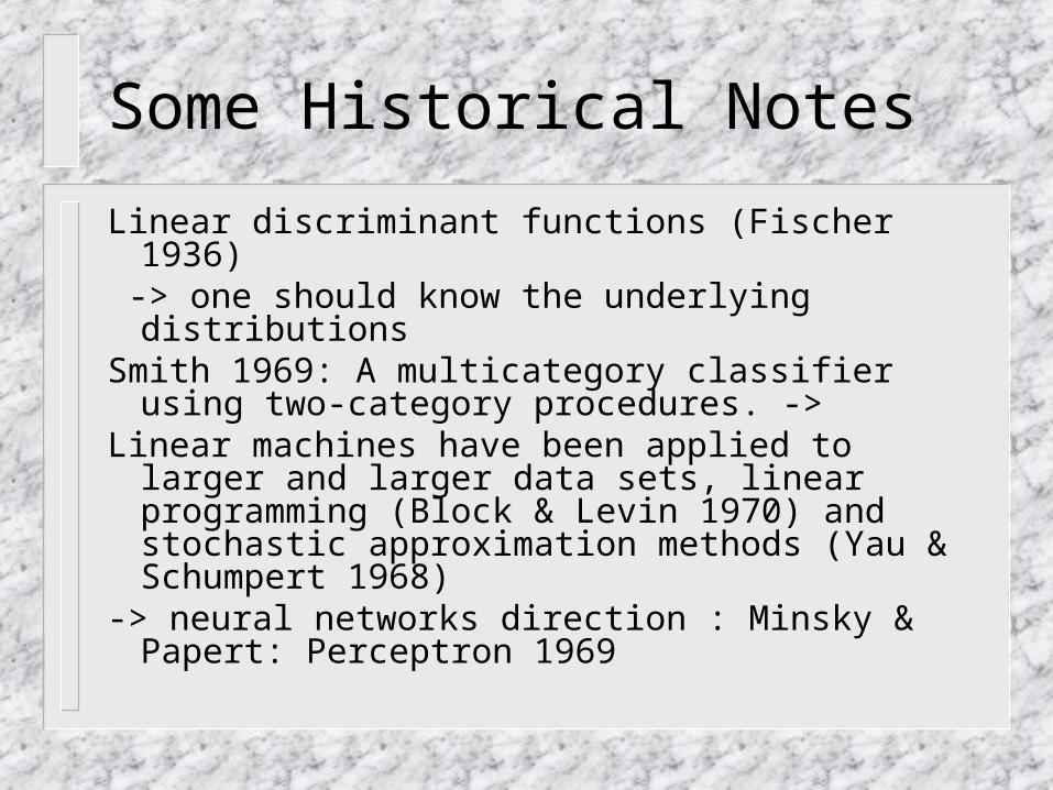
Some Historical Notes

Linear discriminant functions (Fischer 1936) -> one should know the underlying distributionsSmith 1969: A multicategory classifier using two-

category procedures. ->Linear machines have been applied to larger and

larger data sets, linear programming (Block & Levin 1970) and stochastic approximation methods (Yau & Schumpert 1968)

-> neural networks direction : Minsky & Papert: Perceptron 1969

Some Historical Notes

Boser, Guyon,Vapnik 1992 and Schölkopf, Burges, Vapnik 1995 gave the key ideas.

The Kuhn-Tucker construction (1951)

Some Theory

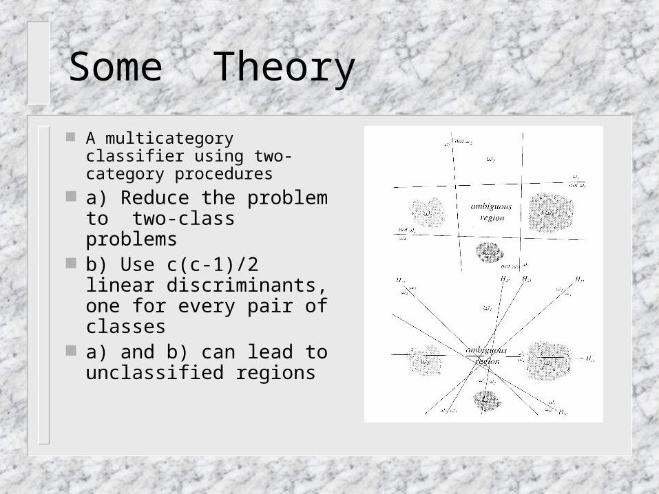
A multicategory classifier using two-category procedures

a) Reduce the problem to two-class problems

b) Use c(c-1)/2 linear discriminants, one for every pair of classes

a) and b) can lead to unclassified regions

Some Theory

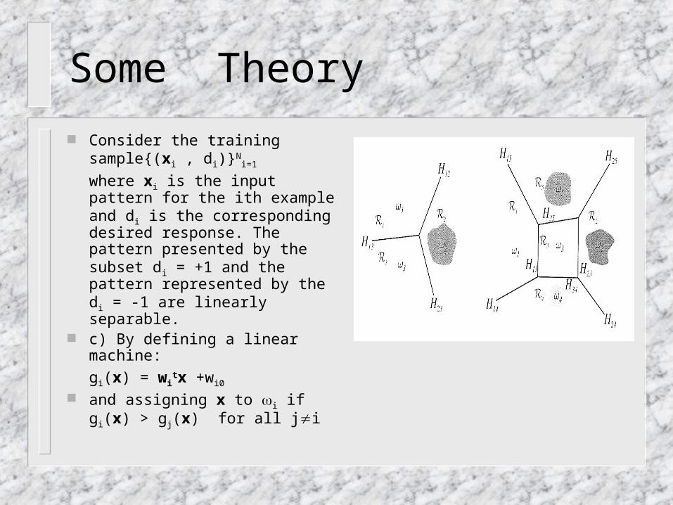
Consider the training sample{(xi , di)}N

i=1

where xi is the input pattern for the ith example and di is the corresponding desired response. The pattern presented by the subset di = +1 and the pattern represented by the di = -1 are linearly separable.

c) By defining a linear machine:

gi(x) = witx +wi0

and assigning x to i if gi(x) > gj(x) for all ji

Some Theory

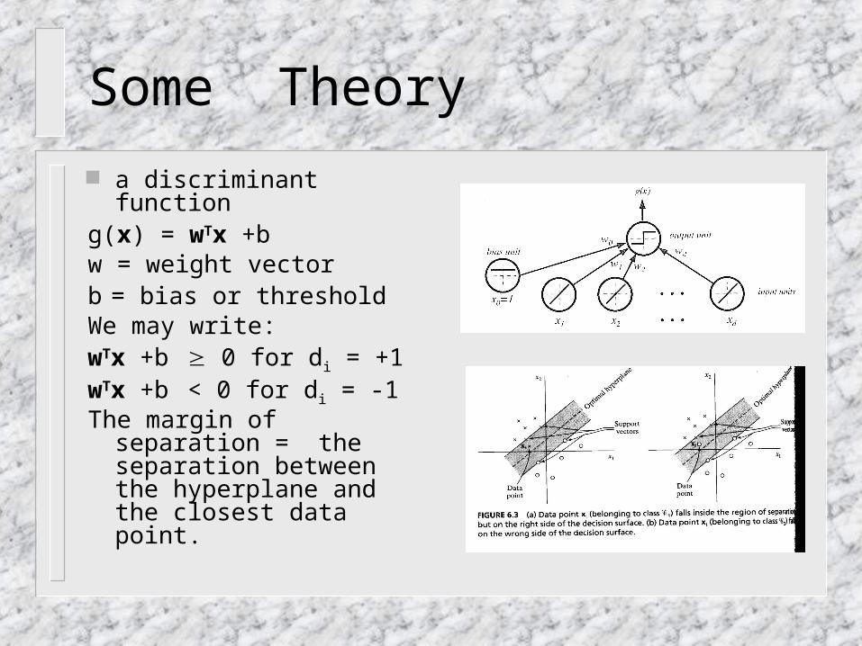
a discriminant functiong(x) = wTx +bw = weight vectorb = bias or thresholdWe may write:wTx +b 0 for di = +1 wTx +b < 0 for di = -1The margin of separation =

the separation between the hyperplane and the closest data point.

Some Theory

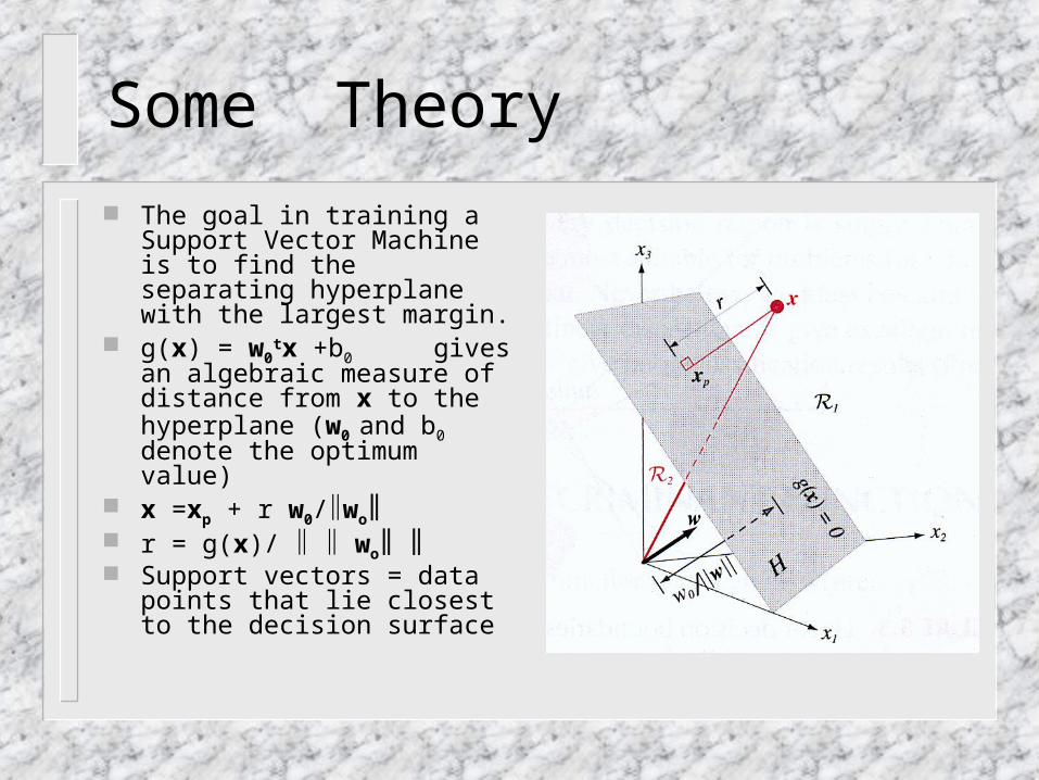
The goal in training a Support Vector Machine is to find the separating hyperplane with the largest margin.

g(x) = w0tx +b0 gives an

algebraic measure of distance from x to the hyperplane (w0

and b0 denote the optimum value)

x =xp + r w0/wo r = g(x)/ wo Support vectors = data points

that lie closest to the decision surface

Some Theory

Now the algebraic distance from the support vector x(s) to the optimal hyperplane is

r = g(x)/ wo This is = 1/ wo if d(s) = +1 or

= - 1/ wo if d(s) = -1 = 2r = 2 / wo The optimal hyperplane is unique (= the maximum

possible separation between positive and negative examples).

Some Theory

Finding the optimal Hyperplane Problem: Given the training sample {(xi ,

di)}Ni=1, find the optimum values of weight

vector w and bias b such that they satisfy the constraint di(wTxi +b) 1 for i = 1,2,…N

and the weight vector w minimizes the cost function: (w) = ½ wTw

Some Theory

The cost function (w) is a convex function of w. The constraints are linear in w. The constrained optimization problem may be

solved by the method of Lagrange multipliers. J(w,b,) = ½ wTw – N

i=1 i[di(wTxi +b)-1] The solution to the constrained optimization

problem is determined by the saddle point of the J(w,b,) (has to beminimized with respect to w and b; has to be maximized with respect to .

Some Theory

Kuhn-Tucker condition and solution of the dual problem. Duality theorem: a) If the primal problem has an optimal

solution, the dual problem has an optimal solution and the corresponding optimal values are equal. b)In order for wo to be an optimal primal solution and o to be an optimal dual solution, it is necessary and sufficient that wo is feasible for the primal problem, and (wo) = J(wo,bo,o) = min w J(w,bo,o)

J(w,b,) = ½ wTw – Ni=1idiwTxi - b N

i=1idi + Ni=1i

Some Theory

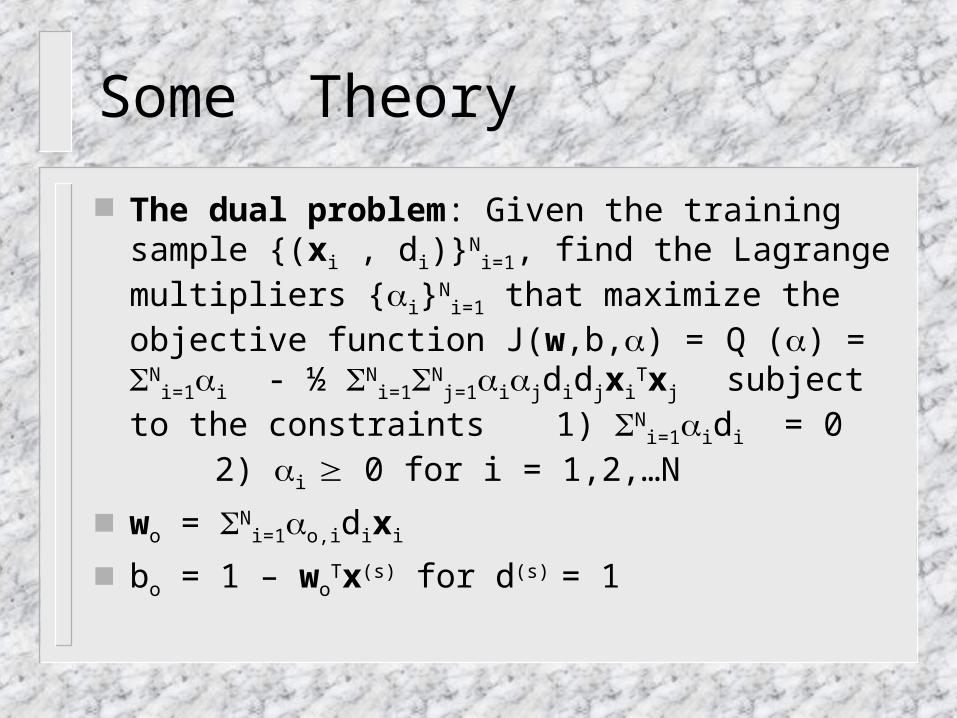
The dual problem: Given the training sample {(xi , di)}N

i=1, find the Lagrange multipliers {i}Ni=1 that

maximize the objective function J(w,b,) = Q () = N

i=1i - ½ Ni=1N

j=1ijdidjxiTxj

subject to the constraints 1) N

i=1idi = 0 2) i 0 for i = 1,2,…N

wo = Ni=1o,idixi

bo = 1 – woTx(s) for d(s) = 1

Some Theory

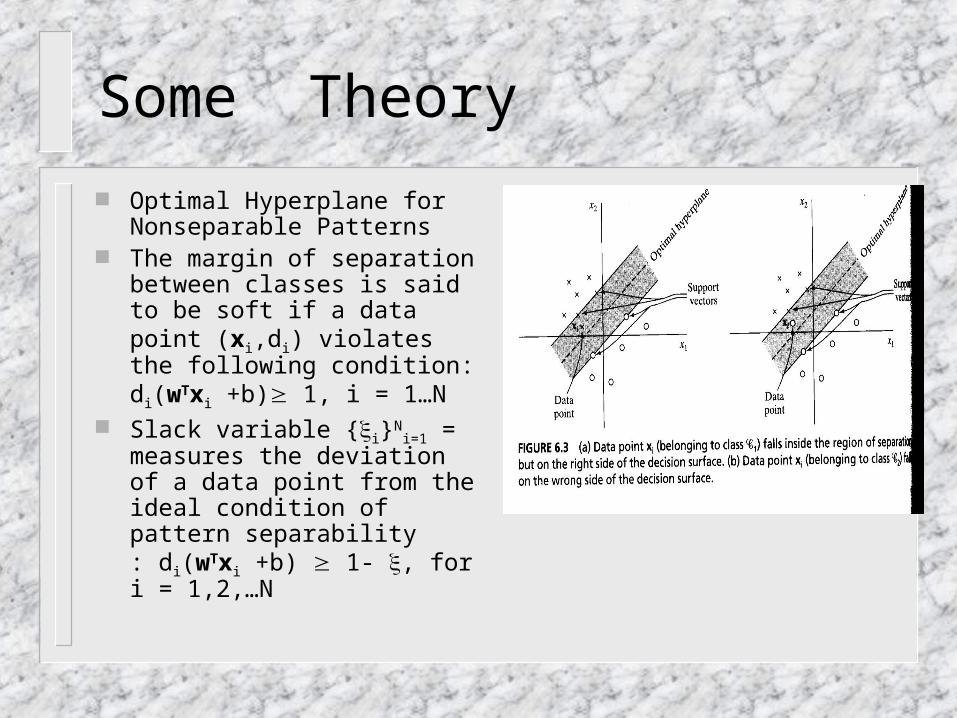
Optimal Hyperplane for Nonseparable Patterns

The margin of separation between classes is said to be soft if a data point (xi,di) violates the following condition: di(wTxi +b) 1, i = 1…N

Slack variable {i}Ni=1 =

measures the deviation of a data point from the ideal condition of pattern separability : di(wTxi +b) 1- , for i = 1,2,…N

Some Theory

Our goal is to find a separating hyperplane for which the missclassification error, averaged on the training set, is minimized.

We may minimize the functional () = N

i=1I(i – 1) with respect to the weight vector w, subject to the constraint di(wTxi +b) 1- , and the constraint w2.

Minimization of () with respect to w is a nonconvex optimization problem (=NP-complete)

Some Theory

We approximate the functional () by writing: (w,) = ½ wTw – C N

i=1i

The first term is related to minimizimg the VC dimension and the second term is an upper bound on the number of test errors.

C is determined either experimentally or analytically by estimating the VC dimension.

Some Theory

Problem: Given the training sample {(xi,di)}Ni=1,

find the optimum values of weight vector w and bias b such that they satisfy the constraint di(wTxi +b)1- i for i = 1,2,…N, i 0 for all i

and such the weight vector w and the slack variables i minimize the cost function: (w,) = ½ wTw – C N

i=1i

where C is a user-specified positive parameter

Some Theory

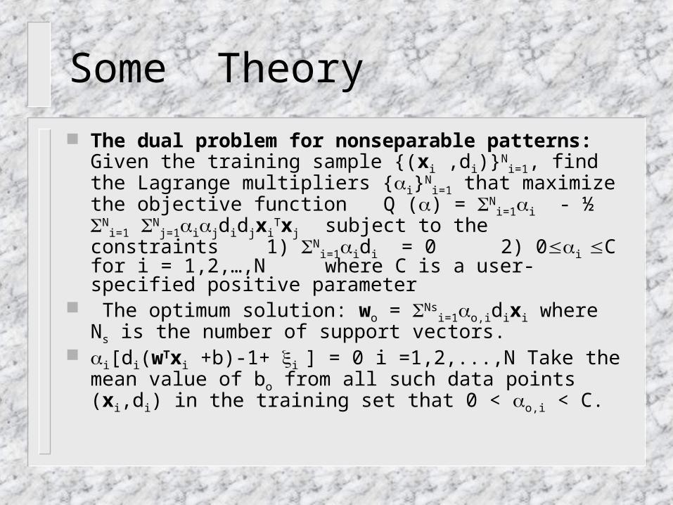
The dual problem for nonseparable patterns: Given the training sample {(xi ,di)}N

i=1, find the Lagrange multipliers {i}N

i=1 that maximize the objective function Q () = N

i=1i - ½ Ni=1 N

j=1ijdidjxiTxj

subject to the constraints 1) N

i=1idi = 0 2) 0i C for i = 1,2,…,N where C is a user-specified positive parameter

The optimum solution: wo = Nsi=1o,idixi where Ns is the

number of support vectors. i[di(wTxi +b)-1+ i ] = 0 i =1,2,...,N Take the mean value of

bo from all such data points (xi,di) in the training set that 0 < o,i < C.

Support Vector Machines

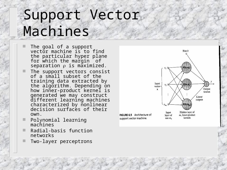
The goal of a support vector machine is to find the particular hyper plane for which the margin of separation is maximized.

The support vectors consist of a small subset of the training data extracted by the algorithm. Depending on how inner-product kernel is generated we may construct different learning machines characterized by nonlinear decision surfaces of their own.

Polynomial learning machines Radial-basis function networks Two-layer perceptrons

Support Vector Machines

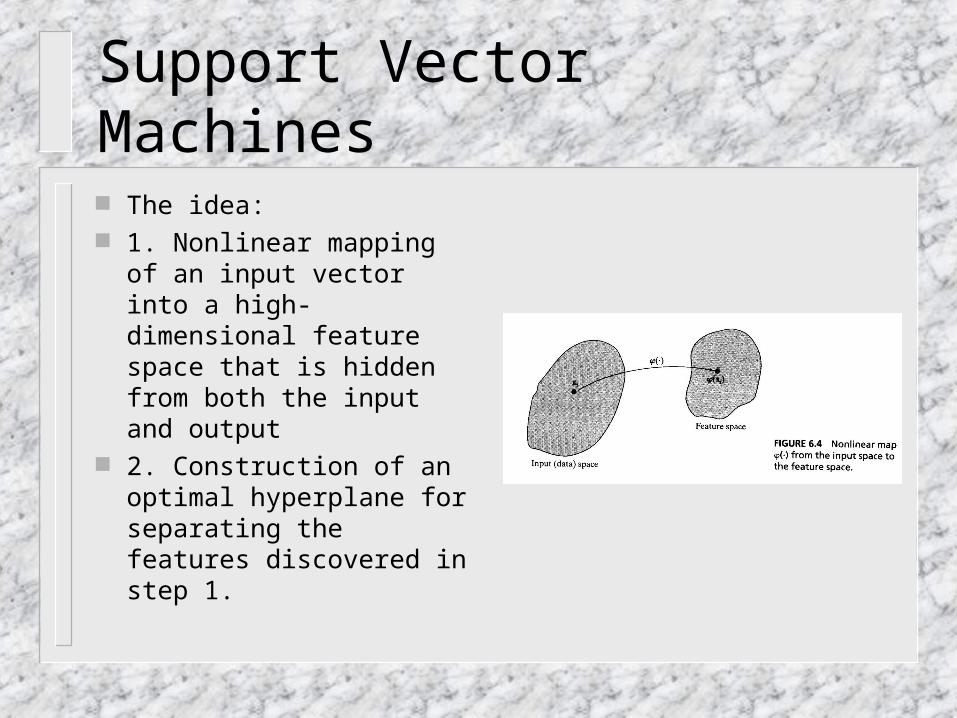
The idea: 1. Nonlinear mapping of

an input vector into a high-dimensional feature space that is hidden from both the input and output

2. Construction of an optimal hyperplane for separating the features discovered in step 1.

Support Vector Machines

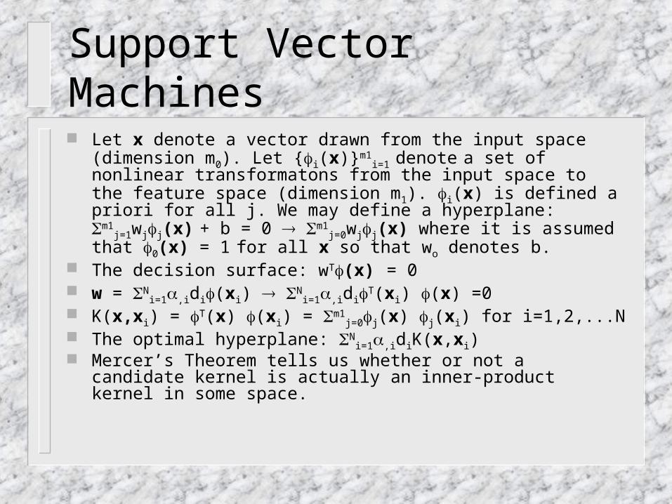
Let x denote a vector drawn from the input space (dimension m0). Let {i(x)}m1

i=1 denote a set of nonlinear transformatons from the input space to the feature space (dimension m1). i(x) is defined a priori for all j. We may define a hyperplane: m1

j=1wjj(x) + b = 0 m1j=0wjj(x) where it is assumed that 0(x) = 1

for all x so that wo denotes b. The decision surface: wT(x) = 0 w = N

i=1,idi(xi) Ni=1,idiT(xi) (x) =0

K(x,xi) = T(x) (xi) = m1j=0j(x) j(xi) for i=1,2,...N

The optimal hyperplane: Ni=1,idiK(x,xi)

Mercer’s Theorem tells us whether or not a candidate kernel is actually an inner-product kernel in some space.

Support Vector Machines

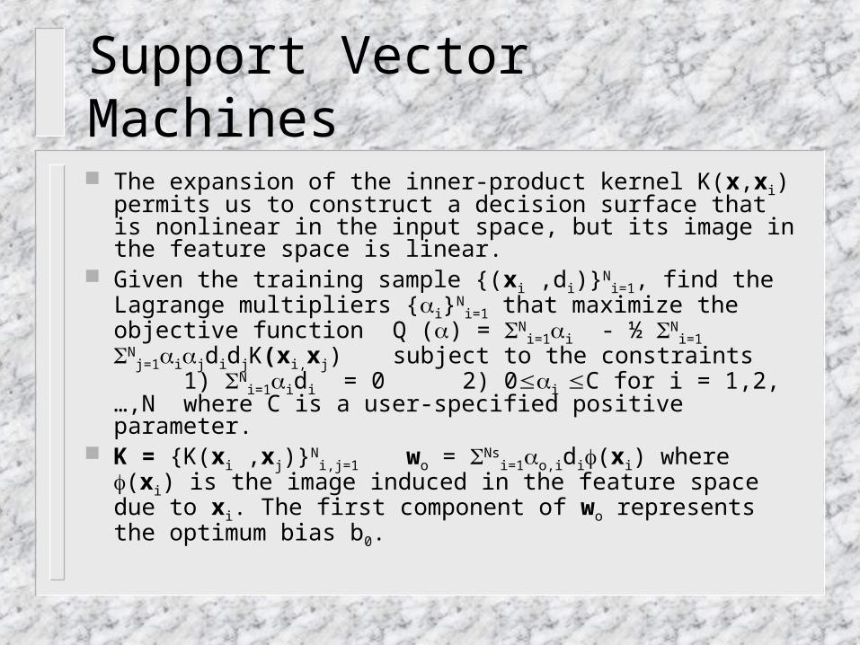
The expansion of the inner-product kernel K(x,xi) permits us to construct a decision surface that is nonlinear in the input space, but its image in the feature space is linear.

Given the training sample {(xi ,di)}Ni=1, find the Lagrange

multipliers {i}Ni=1 that maximize the objective function

Q () = Ni=1i - ½ N

i=1 Nj=1ijdidjK(xi,xj)

subject to the constraints 1) N

i=1idi = 0 2) 0i C for i = 1,2,…,N

where C is a user-specified positive parameter. K = {K(xi ,xj)}N

i,j=1 wo = Nsi=1o,idi(xi) where (xi)

is the image induced in the feature space due to xi. The first component of wo represents the optimum bias b0.

Support Vector Machines

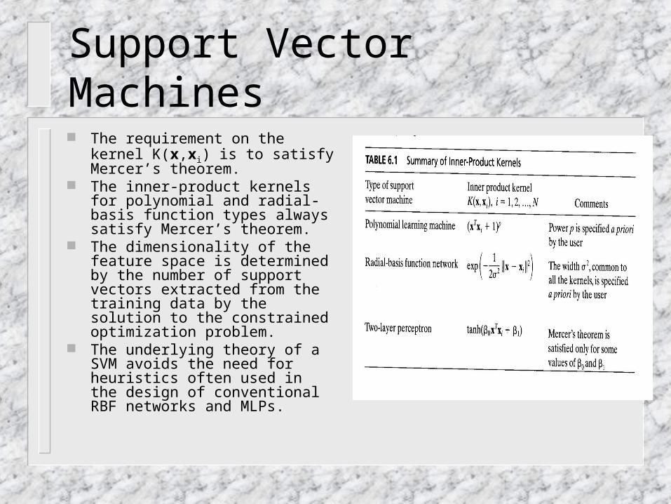
The requirement on the kernel K(x,xi) is to satisfy Mercer’s theorem.

The inner-product kernels for polynomial and radial-basis function types always satisfy Mercer’s theorem.

The dimensionality of the feature space is determined by the number of support vectors extracted from the training data by the solution to the constrained optimization problem.

The underlying theory of a SVM avoids the need for heuristics often used in the design of conventional RBF networks and MLPs.

Support Vector Machines

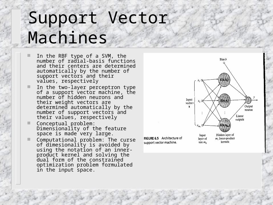
In the RBF type of a SVM, the number of radial-basis functions and their centers are determined automatically by the number of support vectors and their values, respectively

In the two-layer perceptron type of a support vector machine, the number of hidden neurons and their weight vectors are determined automatically by the number of support vectors and their values, respectively

Conceptual problem: Dimensionality of the feature space is made very large.

Computational problem: The curse of dimesionality is avoided by using the notation of an inner-product kernel and solving the dual form of the constrained optimization problem formulated in the input space.

Support Vector Machines

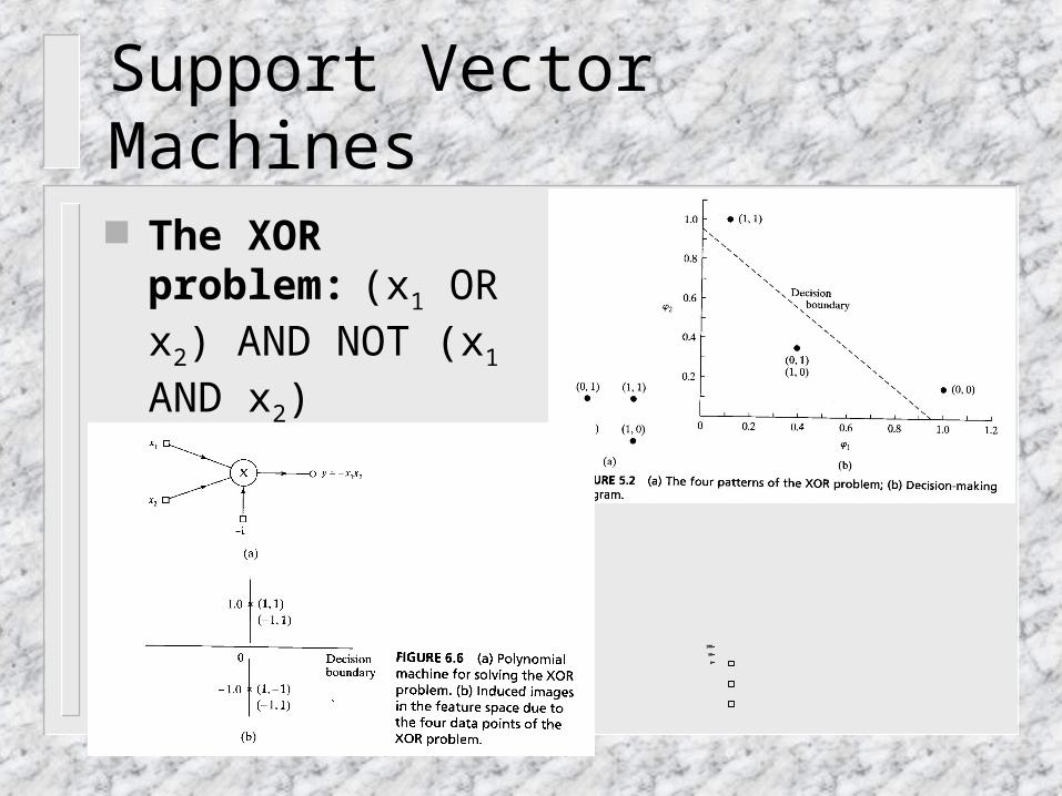
The XOR problem:(x1 OR x2) AND

NOT (x1 AND x2)

0

50

100

1st

Qtr

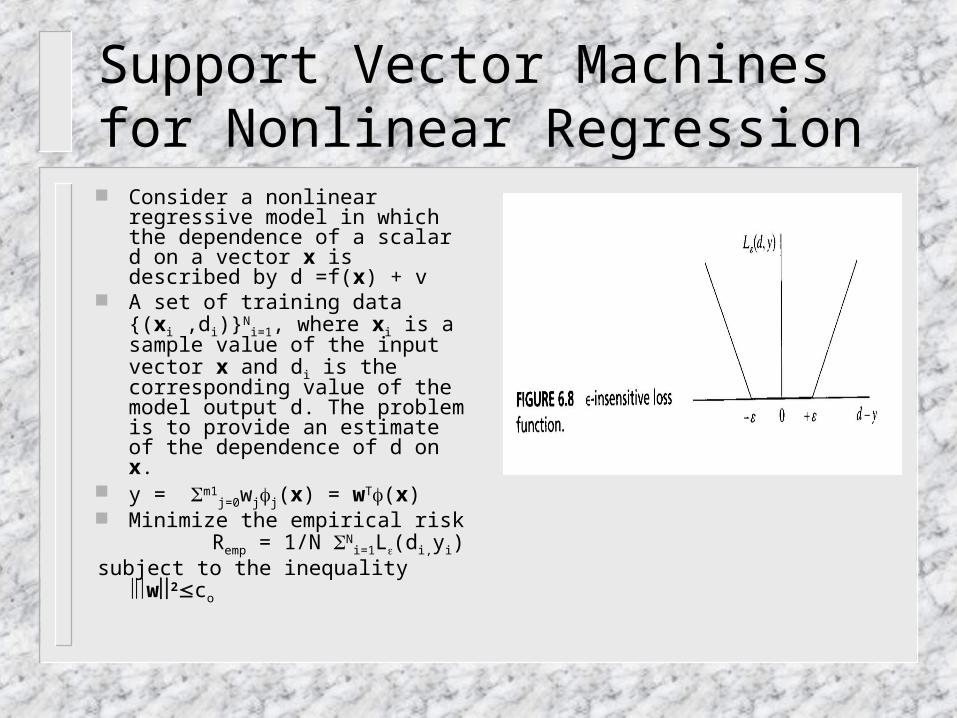
Support Vector Machines for Nonlinear Regression Consider a nonlinear regressive

model in which the dependence of a scalar d on a vector x is described by d =f(x) + v

A set of training data {(xi ,di)}Ni=1,

where xi is a sample value of the input vector x and di is the corresponding value of the model output d. The problem is to provide an estimate of the dependence of d on x.

y = m1j=0wjj(x) = wT(x)

Minimize the empirical risk Remp = 1/N N

i=1L(di,yi) subject to the inequality w2co

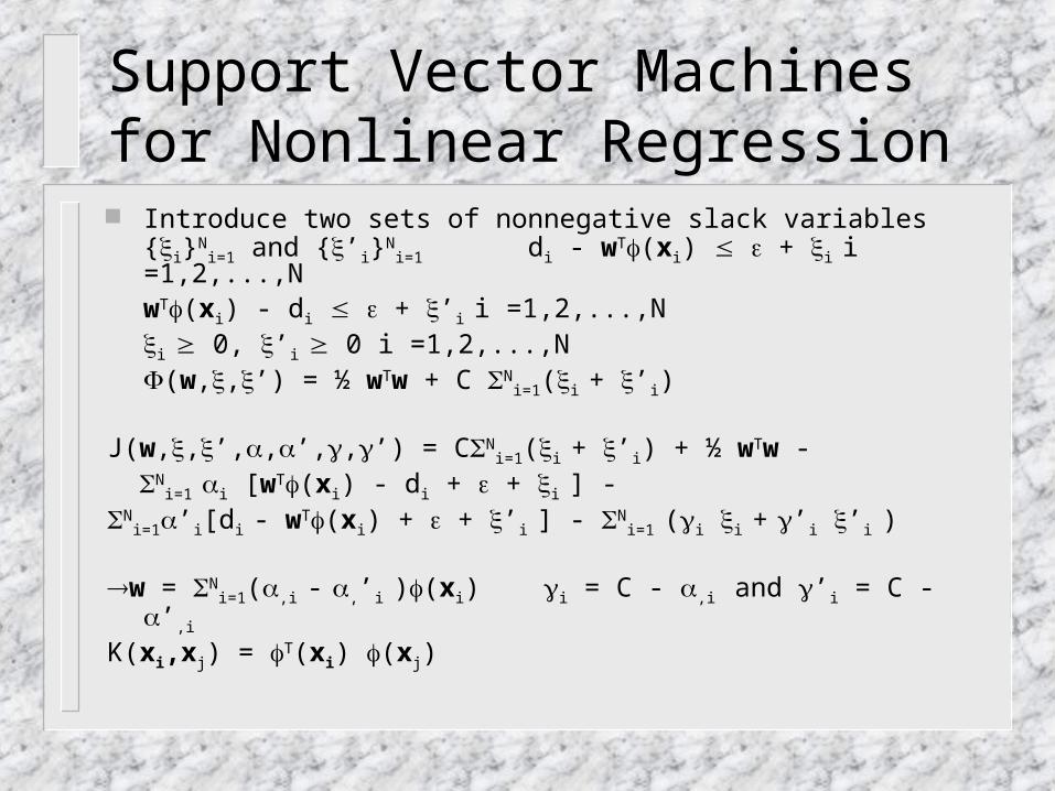
Support Vector Machines for Nonlinear Regression Introduce two sets of nonnegative slack variables {i}N

i=1 and {’i}Ni=1

di - wT(xi) + i i =1,2,...,NwT(xi) - di + ’i i =1,2,...,Ni 0, ’i 0 i =1,2,...,N(w,,’) = ½ wTw + C N

i=1(i + ’i)

J(w,,’,,’,,’) = CNi=1(i + ’i) + ½ wTw -

Ni=1 i [wT(xi) - di + + i ] -

Ni=1’i[di - wT(xi) + + ’i ] - N

i=1 (i i + ’i ’i )

w = Ni=1(,i - ,’i )(xi) i = C - ,i and ’i = C - ’,i

K(xi,xj) = T(xi) (xj)

Support Vector Machines for Nonlinear Regression Given the training sample {(xi ,di)}N

i=1, find the Lagrange multipliers {i}N

i=1 and {’i}Ni=1 that maximize the objective

function Q (i , ’i ) = N

i=1di(i - ’i ) - Ni=1(i + ’i ) - ½ N

i=1 Nj=1

(i - ’i )(j - ’j ) K(xixj) subject to the constraints : 1) N

i=1 (i - ’i ) = 0 2) 0i C for i = 1,2,…,N

0’i C for i = 1,2,…,N where C is a user-specified constant.

The parameters and C are free parameters and selected by the user. They must be tuned simultaneously.

Regression is intrinsically more difficult than pattern classification.

Summary

The SVM is an elegant and highly principled learning method for the design of a feedforward network with a single layer of nonlinear units.

The SVM includes the polynomial learning machine, radial-basis function network, and two-layer perceptron as special cases.

SVM provides a method for controlling model complexity independently of dimensinality.

The SVM learning algorithm operates only in a batch mode. By using a suitable inner-product kernel, the SVM automaticly

computes all the important parameters pertaining to that choice of kernel.

In terms of running time, SVMs are currently slower than other neural networks.