2806 neural computation principal component analysis lecture 8 2005 ari visa
Post on 19-Dec-2015
214 views
TRANSCRIPT
2806 Neural ComputationPrincipal Component Analysis
Lecture 8
2005 Ari Visa

Agenda
Some historical notes Some theory Principal component analysis Conclusions
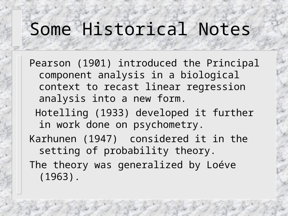
Some Historical Notes
Pearson (1901) introduced the Principal component analysis in a biological context to recast linear regression analysis into a new form.
Hotelling (1933) developed it further in work done on psychometry.
Karhunen (1947) considered it in the setting of probability theory.
The theory was generalized by Loéve (1963).
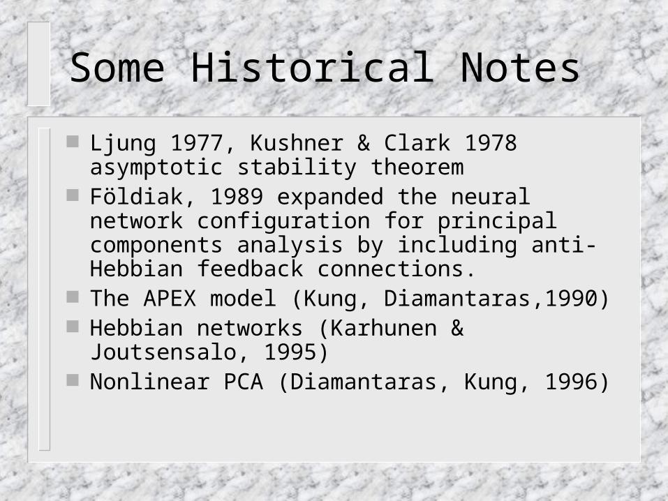
Some Historical Notes
Ljung 1977, Kushner & Clark 1978 asymptotic stability theorem
Földiak, 1989 expanded the neural network configuration for principal components analysis by including anti-Hebbian feedback connections.
The APEX model (Kung, Diamantaras,1990) Hebbian networks (Karhunen & Joutsensalo,
1995) Nonlinear PCA (Diamantaras, Kung, 1996)
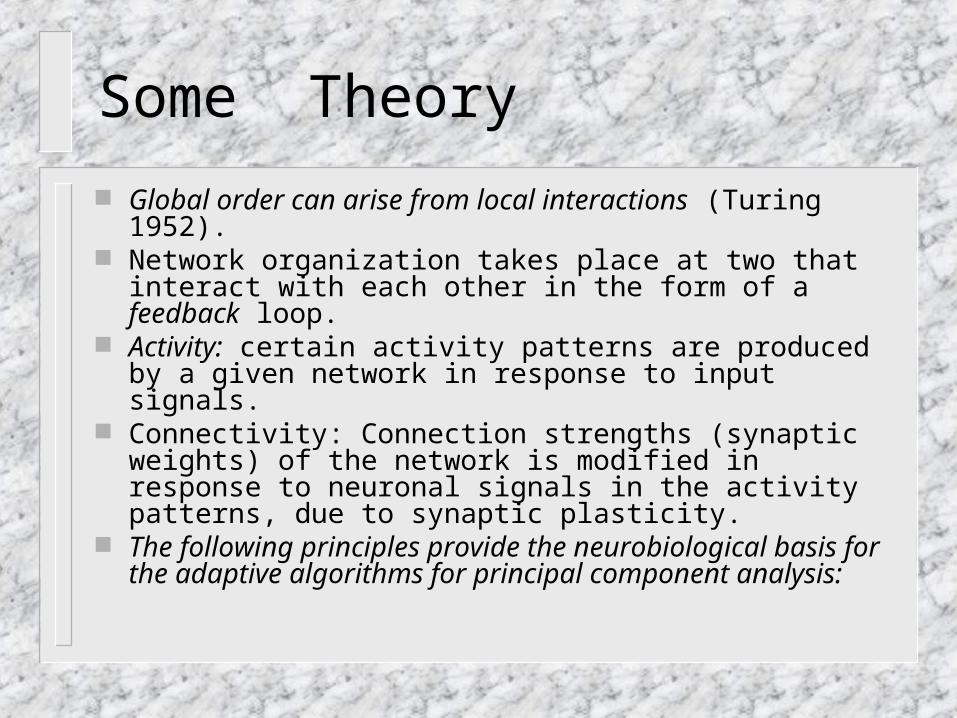
Some Theory
Global order can arise from local interactions (Turing 1952).
Network organization takes place at two that interact with each other in the form of a feedback loop.
Activity: certain activity patterns are produced by a given network in response to input signals.
Connectivity: Connection strengths (synaptic weights) of the network is modified in response to neuronal signals in the activity patterns, due to synaptic plasticity.
The following principles provide the neurobiological basis for the adaptive algorithms for principal component analysis:
Some Theory
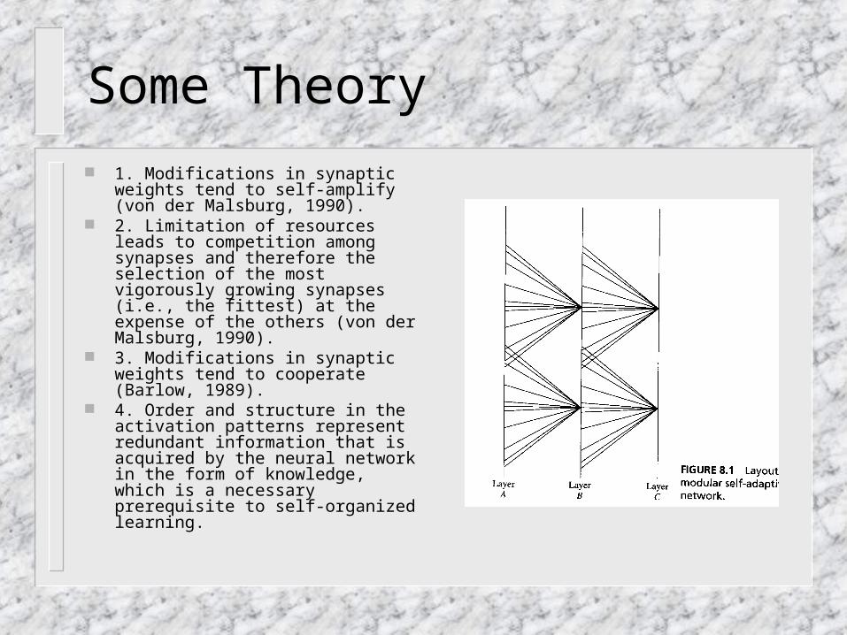
1. Modifications in synaptic weights tend to self-amplify (von der Malsburg, 1990).
2. Limitation of resources leads to competition among synapses and therefore the selection of the most vigorously growing synapses (i.e., the fittest) at the expense of the others (von der Malsburg, 1990).
3. Modifications in synaptic weights tend to cooperate (Barlow, 1989).
4. Order and structure in the activation patterns represent redundant information that is acquired by the neural network in the form of knowledge, which is a necessary prerequisite to self-organized learning.
Some Theory
Consider the transformation from data space to feature space. Is there an invertible linear transform T such that the truncation of Tx is
optimum in the mean-squared error sense? Yes, principle component analysis ( = Karhunen- Loéve transformation)
Let X denote an m-dimensional random vector representing the environment of interest. Let’s assume E[X] = 0;
Let q denote a unit vector of dimension m onto which the vector X is to be projected.
A = XTq = qTX, the projection A is a random variable with a mean and variance related to the statistics of the ramdom vector X.
E[A] = qTE[X] = 0 2 = E[A2] = qTE[XXT]q = qTRq The m-by-m matrix R is the correlation matrix of the random vector X. R is symmetric: RT = R aTRb= bTRa when a and b are any m-by-1 vectors.
Some Theory
Now the problem can be seen as the eigenvalue problem Rq = q
The problem has nontrial solutions (q≠0) only for special values of that are called the eigenvalues of the correlation matrix R.
The associated values of q are called eigenvectors.
R qj = jqj j = 1,2,...,m Let the corresponding eigenvalues be
arranged in decreasing order: 1 > 2 > ... > j >...> m so that 1 = max .
Let the associated eigenvectors be used to construct an m-by-m matrix : Q =[q1, q2, ..., qj , ..., qm]
RQ = Q where is a diagonal matrix defined by the eigenvalues of matrix R: = diag[1 , 2 , ... , j ,..., m ]
The matrix Q is an orthogonal (unitary) matrix in the sense that its column vectors satisfy the conditions of orthonaormality : qi
Tqj = 1, if i=j, 0 if i≠j QTQ=I and QT=Q-1
The orthogonal similarity transformation: QTRQ = or qj
TRqk = j , if k=j, 0 if k≠j
The correlation matrix R may itself be expressed in terms of its eigenvalues and eigenvectors as R = m
i=1 i qi qiT
(the spectral theorem). These are the two equivalent
representations of the eigendecompositions of the correlation matrix R.
Some Theory
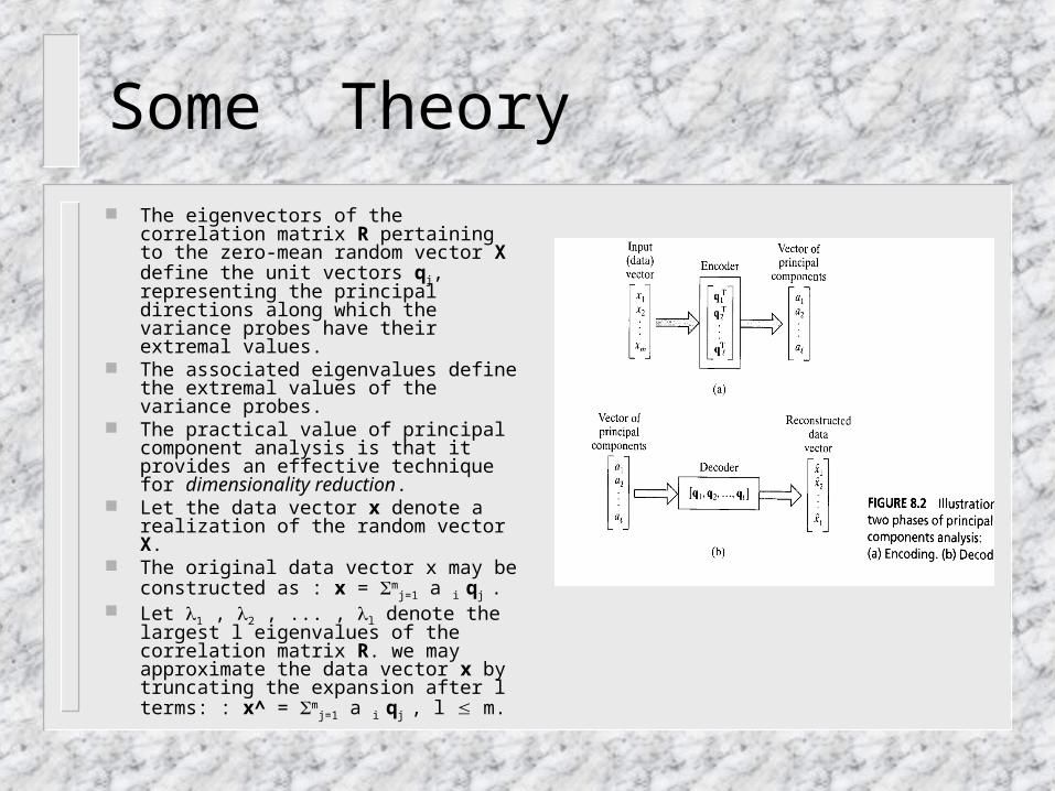
The eigenvectors of the correlation matrix R pertaining to the zero-mean random vector X define the unit vectors qj, representing the principal directions along which the variance probes have their extremal values.
The associated eigenvalues define the extremal values of the variance probes.
The practical value of principal component analysis is that it provides an effective technique for dimensionality reduction.
Let the data vector x denote a realization of the random vector X.
The original data vector x may be constructed as : x = m
j=1 a i qj . Let 1 , 2 , ... , l denote the largest l
eigenvalues of the correlation matrix R. we may approximate the data vector x by truncating the expansion after l terms: : x^ = m
j=1 a i qj , l m.
Some Theory
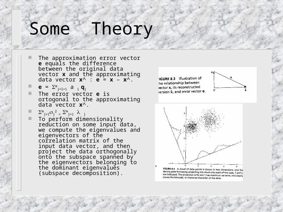
The approximation error vector e equals the difference between the original data vector x and the approximating data vector x^ : e = x – x^.
e = mj=l+1 a i qj
The error vector e is ortogonal to the approximating data vector x^.
mj=1j
2 =
mj=1 j
To perform dimensionality reduction on some input data, we compute the eigenvalues and eigenvectors of the correlation matrix of the input data vector, and then project the data orthogonally onto the subspace spanned by the eigenvectors belonging to the dominant eigenvalues (subspace decomposition).
Principal Component Analysis
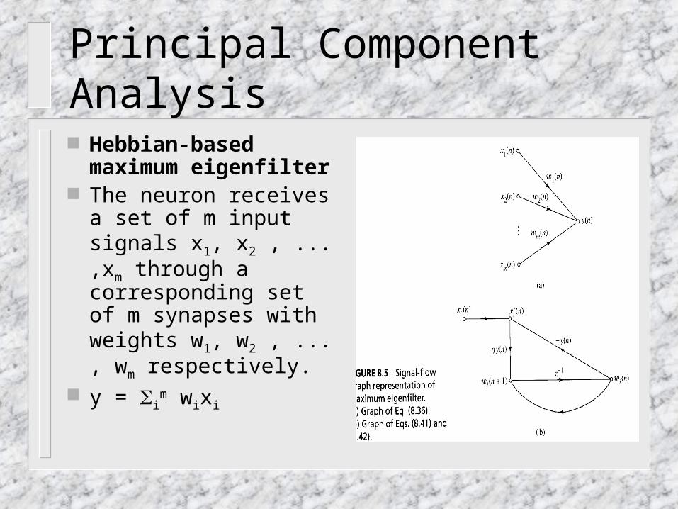
Hebbian-based maximum eigenfilter
The neuron receives a set of m input signals x1, x2 , ... ,xm through a corresponding set of m synapses with weights w1, w2 , ... , wm respectively.
y = im wixi
Principal Component Analysis
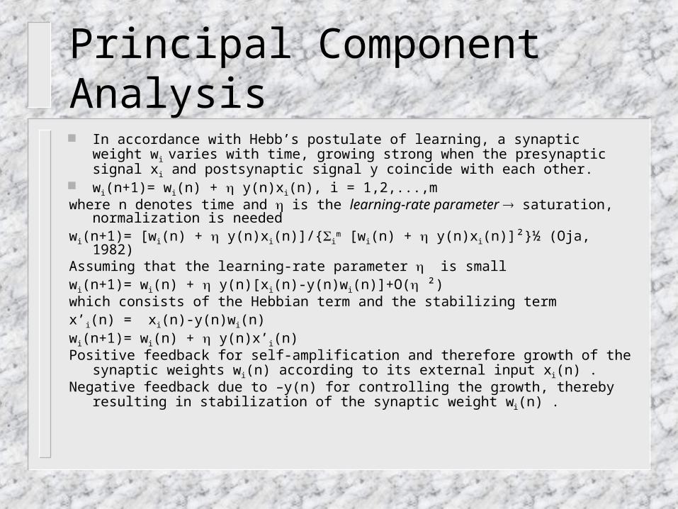
In accordance with Hebb’s postulate of learning, a synaptic weight wi varies with time, growing strong when the presynaptic signal xi and postsynaptic signal y coincide with each other.
wi(n+1)= wi(n) + y(n)xi(n), i = 1,2,...,mwhere n denotes time and is the learning-rate parameter saturation, normalization is
neededwi(n+1)= [wi(n) + y(n)xi(n)]/{i
m [wi(n) + y(n)xi(n)]²}½ (Oja, 1982)Assuming that the learning-rate parameter is smallwi(n+1)= wi(n) + y(n)[xi(n)-y(n)wi(n)]+O( ²)which consists of the Hebbian term and the stabilizing termx’i(n) = xi(n)-y(n)wi(n)wi(n+1)= wi(n) + y(n)x’i(n)Positive feedback for self-amplification and therefore growth of the synaptic weights w i(n)
according to its external input xi(n) .Negative feedback due to –y(n) for controlling the growth, thereby resulting in stabilization
of the synaptic weight wi(n) .
Principal Component Analysis
matrix formulation of the algorithm x(n) = [x1 (n) , x2 (n) , ... ,xm (n) ]T
w(n) = [w1 (n) , w2 (n) , ... ,wm (n) ]T y(n) = xT(n)w(n) = wT(n)x(n) w(n+1)= w(n) + y(n)[x(n)-y(n)w(n)] w(n+1)= w(n) + [x(n)xT(n)w(n) -
wT(n)x(n)xT(n)w(n)w(n)] represents a nonlinear stochastic difference
equation
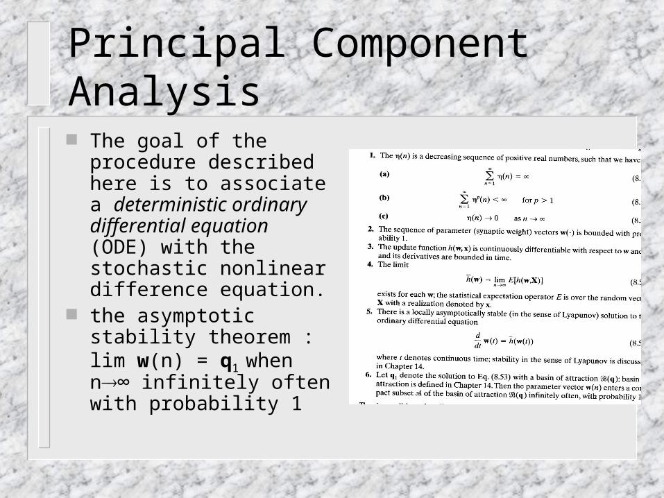
Principal Component Analysis
The goal of the procedure described here is to associate a deterministic ordinary differential equation (ODE) with the stochastic nonlinear difference equation.
the asymptotic stability theorem : lim w(n) = q1
when n∞ infinitely often with probability 1

Principal Component Analysis
A single linear neuron governed by the self-organized learning rule, w(n+1)= w(n) + y(n)[x(n)-y(n)w(n)], converges with probability 1 to a fixed point, which is characterized as follows:
1. The variance of the model output approaches the largest eigenvalue of the correlation matrix R, as shown by lim²(n) = 1 , n∞
2. The synaptic weight vector of the model approches the associated eigenvector, as shown by
lim w(n) = q1 ,, n∞ with lim ||w(n)|| = 1 , n∞
Principal Component Analysis
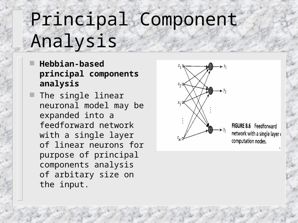
Hebbian-based principal components analysis
The single linear neuronal model may be expanded into a feedforward network with a single layer of linear neurons for purpose of principal components analysis of arbitary size on the input.
Principal Component Analysis
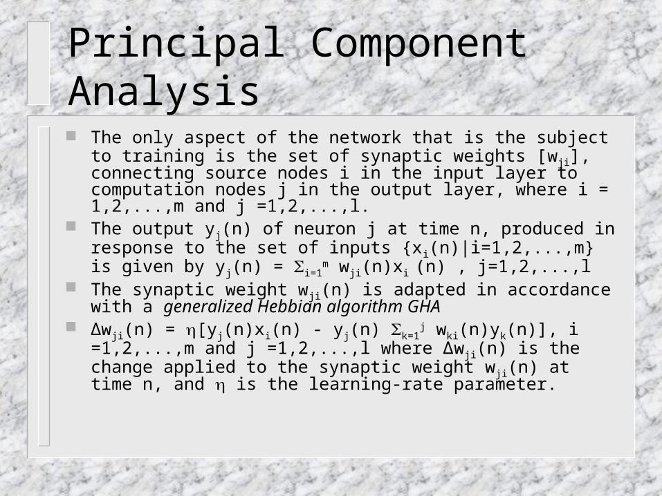
The only aspect of the network that is the subject to training is the set of synaptic weights [wji], connecting source nodes i in the input layer to computation nodes j in the output layer, where i = 1,2,...,m and j =1,2,...,l.
The output yj(n) of neuron j at time n, produced in response to the set of inputs {xi(n)|i=1,2,...,m} is given by yj(n) = i=1
m wji(n)xi (n) , j=1,2,...,l
The synaptic weight wji(n) is adapted in accordance with a generalized Hebbian algorithm GHA
∆wji(n) = [yj(n)xi(n) - yj(n) k=1j wki(n)yk(n)], i =1,2,...,m and j
=1,2,...,l where ∆wji(n) is the change applied to the synaptic weight wji(n) at time n, and is the learning-rate parameter.
Principal Component Analysis
Principal Component Analysis
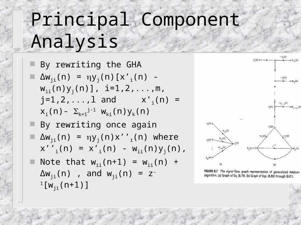
By rewriting the GHA ∆wji(n) = yj(n)[x’i(n) - wii(n)yj(n)],
i=1,2,...,m, j=1,2,...,l and x’i(n) = xi(n)- k=1
j-1 wki(n)yk(n)
By rewriting once again ∆wji(n) = yj(n)x’’i(n) where x’’i(n) =
x’i(n) - wii(n)yj(n),
Note that wii(n+1) = wii(n) + ∆wji(n) , and wji(n) = z-1[wji(n+1)]
Principal Component Analysis
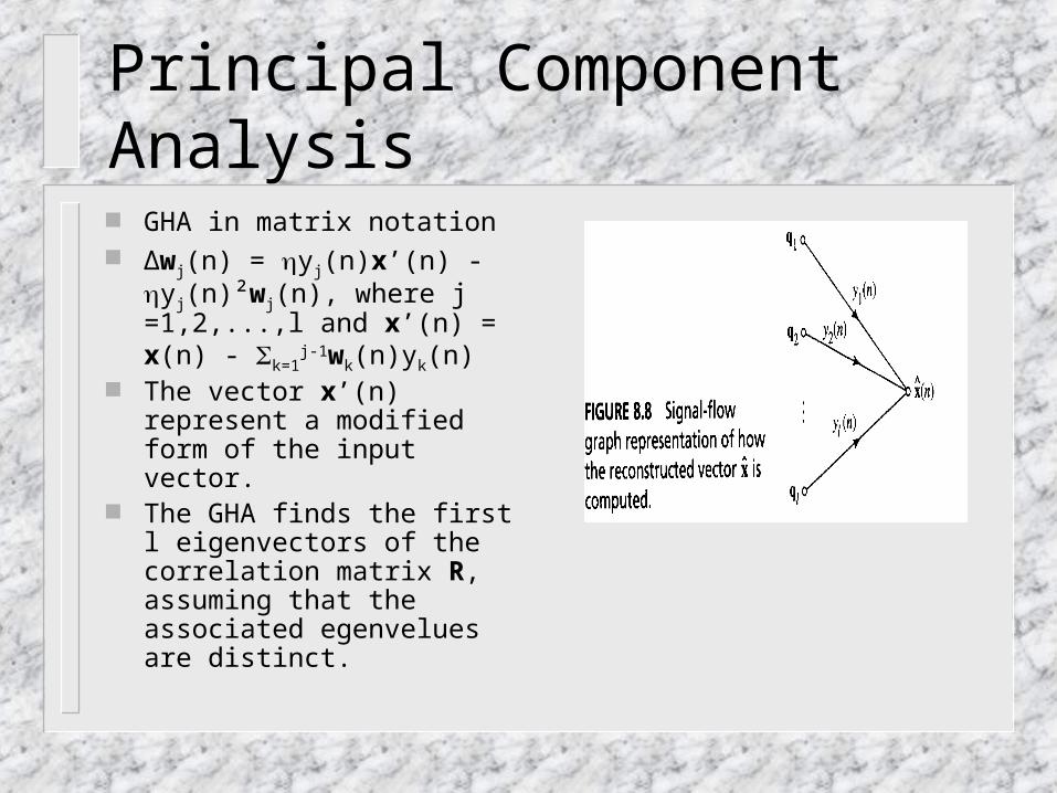
GHA in matrix notation ∆wj(n) = yj(n)x’(n) -
yj(n)²wj(n), where j =1,2,...,l and x’(n) = x(n) - k=1
j-
1wk(n)yk(n) The vector x’(n) represent a
modified form of the input vector.
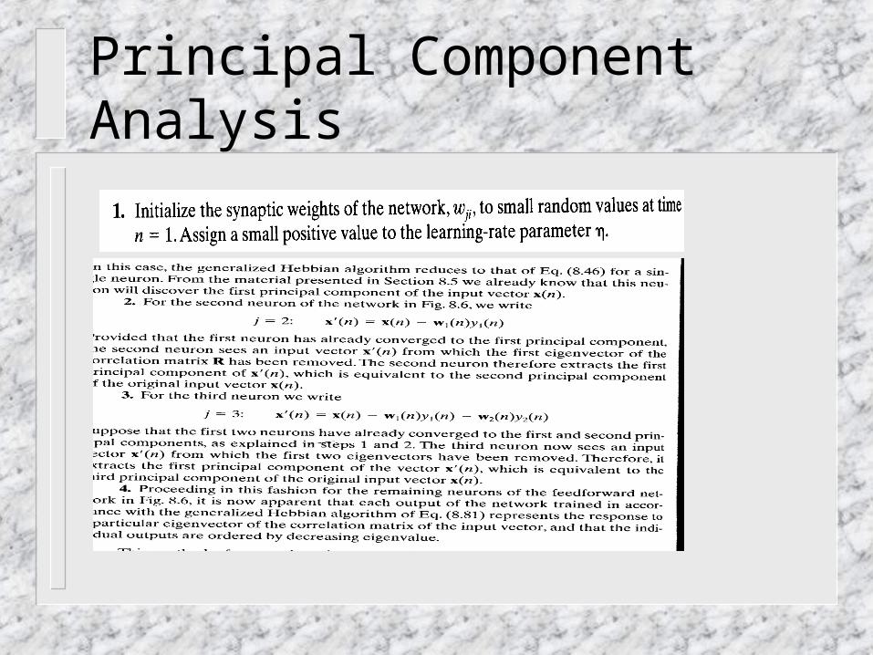
The GHA finds the first l eigenvectors of the correlation matrix R, assuming that the associated egenvelues are distinct.
Principal Component Analysis
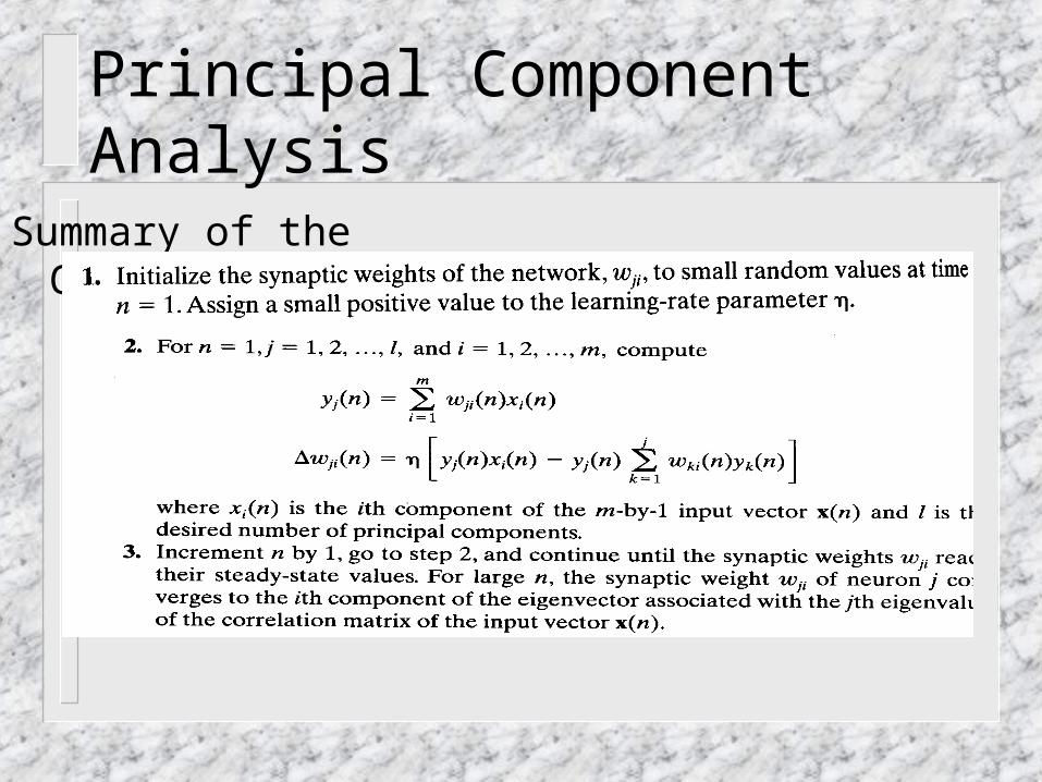
Summary of the GHA
Principal Component Analysis
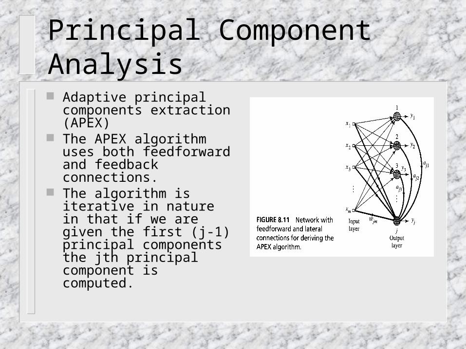
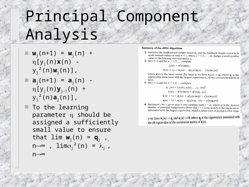
Adaptive principal components extraction (APEX)
The APEX algorithm uses both feedforward and feedback connections.
The algorithm is iterative in nature in that if we are given the first (j-1) principal components the jth principal component is computed.
Principal Component Analysis
Feedforward connections from the input nodes to each of the neurons 1,2,...,j, with j<m. Of particular interest here are the feedforward connections to neuron j, these connections are represented by weight vector wj = [wj1(n),wj2(n), ... ,wjm(n)] T
The feedforward connections operate in accordance with a Hebbian learning rule; they are excitatory and therefore provide for self-amplification.
Lateral connections from the individual outputs of neurons 1,2,...,j-1 to neuron j, thereby applying feedback to the network. These connections are represented by the feedback weight vector aj(n) = [aj1(n),aj2
(n), ... ,ajj-1(n)] T The lateral connections operate in accordance with an anti-Hebbian
learning rule, which has the effect of making them inhibitory.
Principal Component Analysis
The output yj(n) of neuron j is given by yj(n) = wj
T(n)x(n) + ajT(n)yj-1(n)
The feedback signal vector yj-1(n) is defined by the outputs of neurons 1,2,...,j-1
yj-1(n) = [y1(n), y2(n), ... ,ym(n)]T The input vector x(n) is drawn from a stationary process whose correlation
matrix R has distinct eigenvalues arraged in decreased order. It is further assumed that neurons 1,2,...,j-1 of the network have already converged to their respective stable conditions
wk(0) = qk, k=1,2,...,j-1 ak(0) = 0, k=1,2,...,j-1 yj-1(n) = Qx(n) The requirement is to use neuron j in the network to compute the next largest
eigenvalue i of the correlation matrix R of the input vector x(n) and the associated eigenvector q.
Principal Component Analysis
wj(n+1) = wj(n) + [yj(n)x(n) - yj²(n)wj(n)],
aj(n+1) = aj(n) - [yj(n)yj-
1(n) + yj²(n)aj(n)],
To the learning parameter should be assigned a sufficiently small value to ensure that lim wj(n) = qj ,, n∞ , limj²(n) = j , n∞

Some Theory
reestimation algorithms (only feedforward connection)
decorrelating algorithms (both forward and feedback connections)
GHA is a reestimation algorithm because
wj(n+1) = wj(n) + yj(n)[xi(n) – x^j(n)],where x^j(n) is the reestimator
APEX is a decorrelating algorithm
Some Theory
Batch and adaptive methods Eigendecomposition and singular value decomposition
belong to the batch category. GHA and APEX belong to adaptive category. In theory, eigendecomposition is based on the ensemble-
averaged correlation matrix R of a random vector X(n). R^(n) = 1/N n=1
Nx(n)xT(n) From a numerical perspective a better method is to use
singular value decomposition (SVD) by applying it directly to the data matrix. For the set of observations {x(n)}N
n=1, the data matrix is defined by A = [x(1), x(2), ... ,x(N)]T.
Some Theory
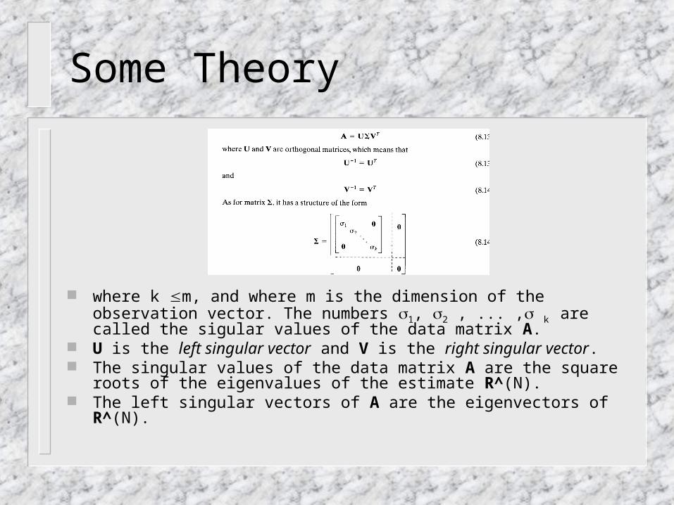
where k m, and where m is the dimension of the observation vector. The numbers 1, 2 , ... , k are called the sigular values of the data matrix A.
U is the left singular vector and V is the right singular vector. The singular values of the data matrix A are the square roots of the
eigenvalues of the estimate R^(N). The left singular vectors of A are the eigenvectors of R^(N).
Some Theory
Adaptive methods work with an arbitrarily large sample size N.
The storage requirement of such methods is relatively modest (intermediate values of eigenvalues and associated eigenvectors do not have to be stored).
In a nonstationary environment, they have an inherent ability to track gradual changes.
0
50
100
1st
Qtr
Principal Component Analysis
Kernel Principal component analysis The computations are performed in a feature space that is nonlinearly
related to the input space. The kernel PCA is nonlinear but the implementation of kernel PCA
relies on linear algebra. Let vector (xj) denote the image of an input vector xj induced in a
feature space defined by the nonlinear map : : Rm0 Rm1, where m0 is the dimensionality of the input space and m1 is the dimensionality of feature space.
Given the set of examples {xi}Nn=1 we have a corresponding set of
feature vectors {(xi}Nn=1 . We may define an m1-by-m1 correlation
matrix in the feature space, denoted by R~. R~ = 1/N N
i=1 (xi) T(xi) R~q~ = ~q~
Principal Component Analysis
Ni=1 N
j=1j (xi) K(xi,xj) = N ~ N
j=1j (xj)where K(xi,xj) is an inner-product kernel
defined in term of the feature vectors.
K²α = N ~Kα where the squared matrix K² denotes the product of K with itself.
Let 1 ≥ 2 ≥ ... ≥ N denote the eigenvalues of the kernel matrix K; that is j = N j~ , j= 1,2, ... , N where j~ is the jth eigenvalue of the correlation matris R~.
Kα = α
Principal Component Analysis
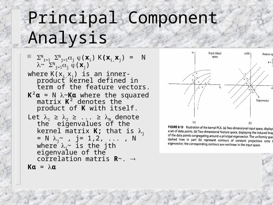
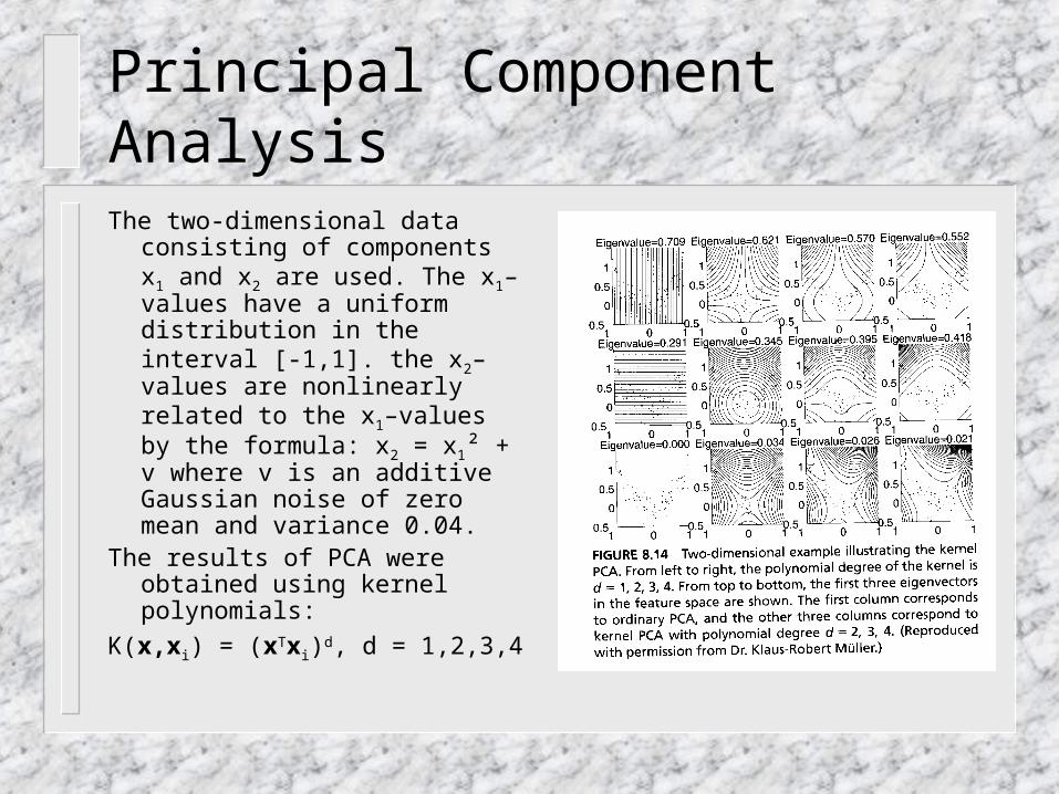
The two-dimensional data consisting of components x1 and x2 are used. The x1–values have a uniform distribution in the interval [-1,1]. the x2–values are nonlinearly related to the x1–values by the formula: x2 = x1² + v where v is an additive Gaussian noise of zero mean and variance 0.04.
The results of PCA were obtained using kernel polynomials:
K(x,xi) = (xTxi)d, d = 1,2,3,4
Principal Component Analysis
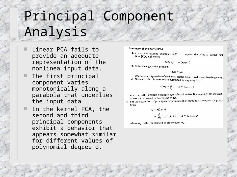
Linear PCA fails to provide an adequate representation of the nonlinea input data.
The first principal component varies monotonically along a parabola that underlies the input data
In the kernel PCA, the second and third principal components exhibit a behavior that appears somewhat similar for different values of polynomial degree d.
Summary
The Hebbian-based algorithms are motivated by ideas taken from neurobiology.
How useful is principal components analysis?If the main objective is to achieve good data
compression while preserving as much information about the inputs as possible
If it happens that there are a few clusters in the data set, then the leading principal axes found by using the principal component analysis will tend to pick projections of clusters with good separations.