2015 fdot highway safety manual user guide · 2015 fdot highway safety manual user guide state...

2015 FDOT

HIGHWAY SAFETY MANUAL

USER GUIDE

STATE SAFETY OFFICE

605 Suwannee Street, MS‐53

Tallahassee, Florida 32399

STATE ROADWAY DESIGN OFFICE

605 Suwannee Street, MS‐32

Tallahassee, Florida 32399

FDOT HIGHWAY SAFETY MANUAL USER’S GUIDE

Contact Information

Jeremy W. Fletcher, P.E., P.S.M. Roadway Quality Assurance Administrator Florida Department of Transportation 605 Suwannee Street - MS 32 Tallahassee, Florida 32399-0450 (850) 414-4320 [email protected] Joseph B. Santos, P.E. State Safety Engineer Florida Department of Transportation 605 Suwannee Street - MS 53 Tallahassee, Florida 32399-0450 (850) 414-4097 [email protected] Alan El-Urfali, P.E. Traffic Engineering and Operations Office Florida Department of Transportation 605 Suwannee Street - MS 36 Tallahassee, Florida 32399-0450 (850) 921-7361 [email protected] Martha Hodgson Systems Planning Office Florida Department of Transportation 605 Suwannee Street - MS 19 Tallahassee, Florida 32399-045 (850) 414-4804 [email protected]

Catherine Bradley, P.E. Environmental Management Office Florida Department of Transportation 605 Suwannee Street - MS 37 Tallahassee, Florida 32399-045 (850) 414-4271 [email protected] Victor Muchuruza, PhD, P.E. P.T.O.E. State Environmental Management Office Florida Department of Transportation 605 Suwannee Street - MS 37 Tallahassee, Florida 32399-045 (850) 414-4902 [email protected] Mary Jane Hayden, P.E. Production Support Office Florida Department of Transportation 605 Suwannee Street - MS 40 Tallahassee, Florida 32399-045 (850) 414-4783 [email protected] Gina Bonyani Systems Planning Office Florida Department of Transportation 605 Suwannee Street - MS 19 Tallahassee, Florida 32399-045 (850) 414-4707 [email protected]

mailto:[email protected]













Table of Contents

Chapter 1 Introduction

Chapter 2 Highway Safety Manual Terms and Concepts

Chapter 3 The Highway Safety Manual Predictive Method

Chapter 4 Selecting an Appropriate CMF of CRF

Chapter 5 Countermeasure CMFs

Chapter 6 Additional Resources

FDOT HIGHWAY SAFETY MANUAL USER’S GUIDE – CHAPTER 1 - INTRODUCTION

1-1

Chapter 1

Introduction

1.1 Purpose

The Highway Safety Manual (HSM) provides statistical tools which can be used from the Systems Planning Process through Operations and Maintenance. There are safety, operational, and financial benefits from the use of these tools. The FDOT HSM User’s Guide provides an abbreviated overview for practitioners of the HSM. The intent is to provide guidance on the application of the HSM. FDOT Transportation Planners, Engineers and other Decision Makers are encouraged to implement this manual, whenever possible, on FDOT Projects.

1.2 Highway Safety Manual

The Highway Safety Manual (HSM) is a resource that provides safety knowledge and tools in a useful form to facilitate improved decision making based on safety performance. The HSM is an AASHTO manual that includes methodologies to quantitatively predict a facility’s safety performance. The “Predictive Method” in the HSM provides equations (Safety Performance Functions) that statistically predict the number of crashes on rural two-lane roads, rural multilane roads, urban/suburban roads, urban/rural freeways, and ramps with specific geometric features and traffic volumes for a given period of time.

The HSM consists of 3 volumes (published in 2010) and a supplement (published in 2014). It is divided into four Parts (A, B, C, & D) as follows:

• Volume 1 o Part A - Introduction, Human Factors, and Fundamentals

Purpose and Scope of HSM Chapters 1 – 3

• Chapter 1 – Introduction and Overview • Chapter 2 – Human Factors • Chapter 3 - Fundamentals

o Part B - Roadway Safety Management Process Existing Roadways Steps

• Monitor and Reduce Crash o Frequency o Severity

Chapters 4 – 9 • Chapter 4 – Network Screening • Chapter 5 – Diagnosis • Chapter 6 – Select Countermeasures • Chapter 7 – Economic Appraisal

FDOT HIGHWAY SAFETY MANUAL USER’S GUIDE – CHAPTER 1 - INTRODUCTION

1-2

• Chapter 8 – Prioritize • Chapter 9 – Safety Effectiveness Evaluation

• Volume 2 and Supplement o Part C

Predictive Method Chapters 10 – 12 (Volume 2)

• Chapter 10 - Rural Two-lane Roads • Chapter 11 - Rural Multilane Roads • Chapter 12 - Urban/Suburban Arterials

Chapters 18 – 19 (Supplement) • Chapter 18 - Freeways • Chapter 19 - Ramps

• Volume 3 o Part D

Presents information regarding the effects of various countermeasures Chapters 13 – 17

• Chapter 13 – Roadway Segments • Chapter 14 – Intersections • Chapter 15 – Interchanges • Chapter 16 – Special Facilities • Chapter 17 – Road Networks

Crash Modification Factors (CMFs) are found in Part C and Part D of the HSM

FDOT HIGHWAY SAFETY MANUAL USER’S GUIDE – CHAPTER 2 –HIGHWAY SAFETY MANUAL TERMS AND CONCEPTS

2-1

Chapter 2

Highway Safety Manual Terms and Concepts

2.1 Safety Performance Function (SPF)

Safety Performance Functions (SPFs) are statistical models (equations) used to estimate the average crash frequency for a specific site, based on traffic volume and general roadway characteristics. The crashes that are estimated using SPFs are referred to as the Predicted Number of Crashes (Npredicted).

The SPF equations are the basis of the Predictive Method and were developed in HSM-related multi-state research from the most complete and consistent available data sets. However, the general level of crash frequencies may vary substantially from one jurisdiction to another for a variety of reasons including climate, driver populations, animal populations, crash reporting thresholds, and crash reporting system procedures. Therefore, for the Part C predictive models to provide results that are meaningful and accurate for each jurisdiction, it is important that the SPFs be calibrated for application in each jurisdiction.

2.2 Base Conditions

The base conditions may also be thought of as the default condition for each SPF. The base conditions are the conditions for which each SPF was developed. The base condition is different for each SPF and is specified in the HSM Chapters 10, 11, 12, 18, and 19. The base condition is not necessarily a perfect or ideal condition; it is a reflection of the data available to the statisticians at the time the SPF was developed.

2.3 Observed Crash

Observed crashes are historical crashes that have occurred within the limits of the site being investigated. Crash Reports should be obtained from the FDOT State Safety Office and also the local law enforcement agency for the years being analyzed.

2.4 Regression-to-the-Mean

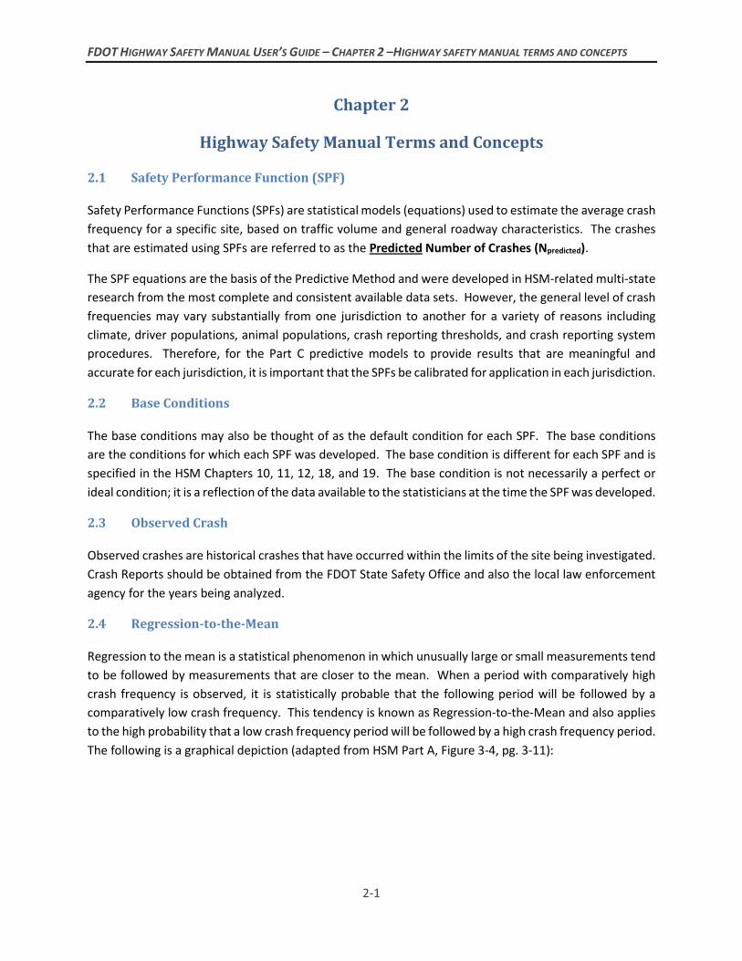
Regression to the mean is a statistical phenomenon in which unusually large or small measurements tend to be followed by measurements that are closer to the mean. When a period with comparatively high crash frequency is observed, it is statistically probable that the following period will be followed by a comparatively low crash frequency. This tendency is known as Regression-to-the-Mean and also applies to the high probability that a low crash frequency period will be followed by a high crash frequency period. The following is a graphical depiction (adapted from HSM Part A, Figure 3-4, pg. 3-11):


2-2

Figure 2-1 Regression-to-the-Mean Bias

(Ref: Figure 3-4 – 2010 AASHTO Highway Safety Manual)

2.5 Empirical-Bayes (EB) Method

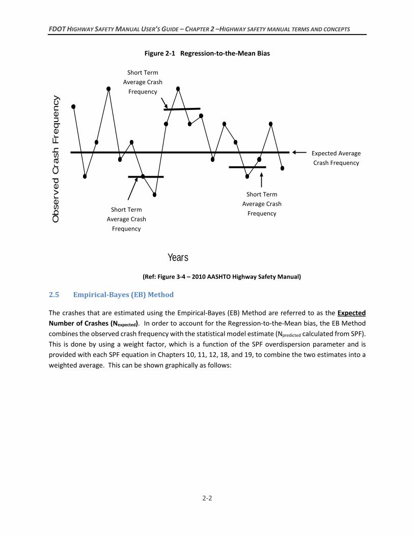
The crashes that are estimated using the Empirical-Bayes (EB) Method are referred to as the Expected Number of Crashes (Nexpected). In order to account for the Regression-to-the-Mean bias, the EB Method combines the observed crash frequency with the statistical model estimate (Npredicted calculated from SPF). This is done by using a weight factor, which is a function of the SPF overdispersion parameter and is provided with each SPF equation in Chapters 10, 11, 12, 18, and 19, to combine the two estimates into a weighted average. This can be shown graphically as follows:

Years

Obse

rved C

rash

Fre

quency

Short Term Average Crash

Frequency


Expected Average Crash Frequency



Frequency


Frequency


Frequency

Expected Average Crash Frequency


2-3

Figure 2-2 EB Method Concept

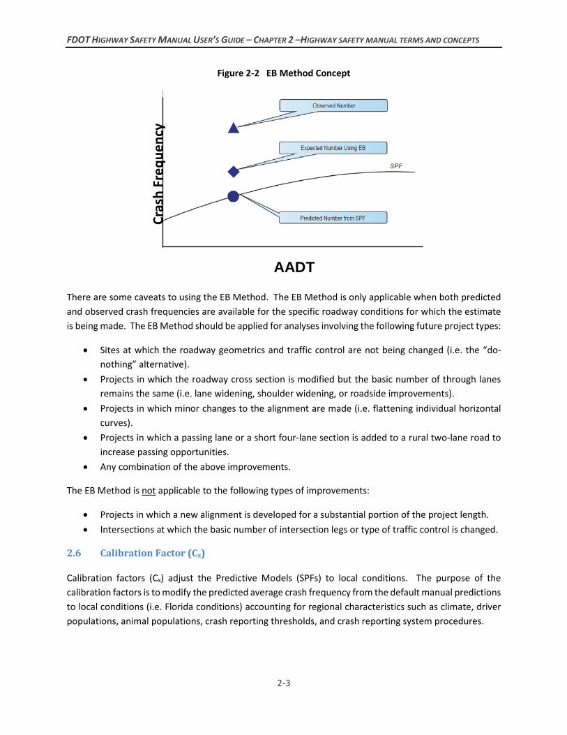
There are some caveats to using the EB Method. The EB Method is only applicable when both predicted and observed crash frequencies are available for the specific roadway conditions for which the estimate is being made. The EB Method should be applied for analyses involving the following future project types:

• Sites at which the roadway geometrics and traffic control are not being changed (i.e. the “do-nothing” alternative).

• Projects in which the roadway cross section is modified but the basic number of through lanes remains the same (i.e. lane widening, shoulder widening, or roadside improvements).

• Projects in which minor changes to the alignment are made (i.e. flattening individual horizontal curves).

• Projects in which a passing lane or a short four-lane section is added to a rural two-lane road to increase passing opportunities.

• Any combination of the above improvements.

The EB Method is not applicable to the following types of improvements:

• Projects in which a new alignment is developed for a substantial portion of the project length. • Intersections at which the basic number of intersection legs or type of traffic control is changed.

2.6 Calibration Factor (Cx)

Calibration factors (Cx) adjust the Predictive Models (SPFs) to local conditions. The purpose of the calibration factors is to modify the predicted average crash frequency from the default manual predictions to local conditions (i.e. Florida conditions) accounting for regional characteristics such as climate, driver populations, animal populations, crash reporting thresholds, and crash reporting system procedures.

AADT

Cras

h Fr

eque

ncy


2-4

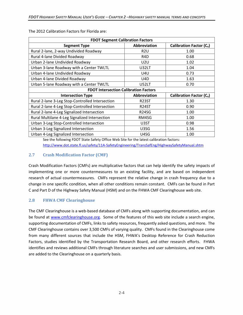
The 2012 Calibration Factors for Florida are:

FDOT Segment Calibration Factors Segment Type Abbreviation Calibration Factor (Cx)

Rural 2-lane, 2-way Undivided Roadway R2U 1.00 Rural 4-lane Divided Roadway R4D 0.68 Urban 2-lane Undivided Roadway U2U 1.02 Urban 3-lane Roadway with a Center TWLTL U32LT 1.04 Urban 4-lane Undivided Roadway U4U 0.73 Urban 4-lane Divided Roadway U4D 1.63 Urban 5-lane Roadway with a Center TWLTL U52LT 0.70

FDOT Intersection Calibration Factors Intersection Type Abbreviation Calibration Factor (Cx)

Rural 2-lane 3-Leg Stop-Controlled Intersection R23ST 1.30 Rural 2-lane 4-Leg Stop-Controlled Intersection R24ST 0.90 Rural 2-lane 4-Leg Signalized Intersection R24SG 1.00 Rural Multilane 4-Leg Signalized Intersection RM4SG 1.00 Urban 3-Leg Stop-Controlled Intersection U3ST 0.98 Urban 3-Leg Signalized Intersection U3SG 1.56 Urban 4-Leg Signalized Intersection U4SG 1.00

See the following FDOT State Safety Office Web Site for the latest calibration factors: http://www.dot.state.fl.us/safety/11A-SafetyEngineering/TransSafEng/HighwaySafetyManual.shtm

2.7 Crash Modification Factor (CMF)

Crash Modification Factors (CMFs) are multiplicative factors that can help identify the safety impacts of implementing one or more countermeasures to an existing facility, and are based on independent research of actual countermeasures. CMFs represent the relative change in crash frequency due to a change in one specific condition, when all other conditions remain constant. CMFs can be found in Part C and Part D of the Highway Safety Manual (HSM) and on the FHWA CMF Clearinghouse web site.

2.8 FHWA CMF Clearinghouse

The CMF Clearinghouse is a web-based database of CMFs along with supporting documentation, and can be found at www.cmfclearinghouse.org. Some of the features of this web site include a search engine, supporting documentation of CMFs, links to safety resources, frequently asked questions, and more. The CMF Clearinghouse contains over 3,500 CMFs of varying quality. CMFs found in the Clearinghouse come from many different sources that include the HSM, FHWA’s Desktop Reference for Crash Reduction Factors, studies identified by the Transportation Research Board, and other research efforts. FHWA identifies and reviews additional CMFs through literature searches and user submissions, and new CMFs are added to the Clearinghouse on a quarterly basis.

http://www.dot.state.fl.us/safety/11A-SafetyEngineering/TransSafEng/HighwaySafetyManual.shtm

http://www.cmfclearinghouse.org/


2-5

2.9 Distinction of Various CMFs

HSM Part C CMFs (HSM Chapters 10, 11, 12, 18, and 19) • Developed to adjust for differences between the base conditions and the existing site-

specific conditions (i.e. existing lane width is less than 12 ft., which is the base condition) • Originate from the research database from which the SPFs were developed • Available in Part D

HSM Part D CMFs (HSM Chapters 13 – 17) • Used for specific countermeasures that are not adjustments to the base conditions (i.e.

implement time-limited parking restrictions, which has no associated base condition) • Reviewed and approved by the HSM Task Force • Applicable to any site analysis • Includes Part C CMFs, as well as others

FHWA Clearinghouse CMFs • Similar to Part D CMFs, these are also used for specific countermeasures that are not

adjustments to the base conditions • Reviewed and approved by FHWA CMF Clearinghouse Staff • Applicable to any site analysis • Includes Part C CMFs, Part D CMFs, and non-HSM CMFs

2.10 Crash Reduction Factors

Crash Reduction Factors (CRFs) are also multiplicative factors that can help identify the safety impacts of implementing one or more countermeasures to an existing facility, and are based on independent research of actual countermeasures. A CRF is the percentage of crash reduction that may be expected after implementing a countermeasure. FDOT’s CRFs can be found on the following web site: http://www.dot.state.fl.us/rddesign/QA/Tools.shtm.

2.11 CMFs versus CRFs

CMFs are used to predict the number of crashes after implementing a countermeasure, whereas CRFs are used to predict the percent reduction in crashes resulting from implementing a countermeasure. Mathematically speaking: CMF = 1 – (CRF / 100).

http://www.dot.state.fl.us/rddesign/QA/Tools.shtm


2-6

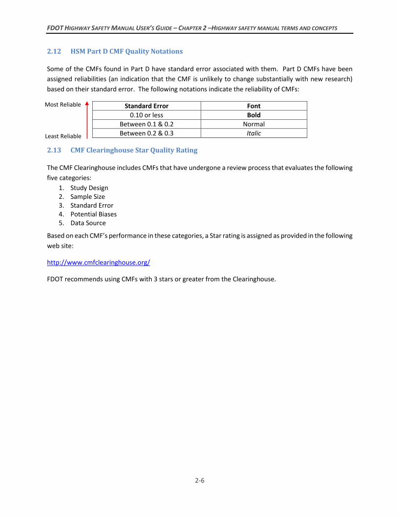
2.12 HSM Part D CMF Quality Notations

Some of the CMFs found in Part D have standard error associated with them. Part D CMFs have been assigned reliabilities (an indication that the CMF is unlikely to change substantially with new research) based on their standard error. The following notations indicate the reliability of CMFs:

Standard Error Font 0.10 or less Bold

Between 0.1 & 0.2 Normal Between 0.2 & 0.3 Italic

2.13 CMF Clearinghouse Star Quality Rating

The CMF Clearinghouse includes CMFs that have undergone a review process that evaluates the following five categories:

1. Study Design 2. Sample Size 3. Standard Error 4. Potential Biases 5. Data Source

Based on each CMF’s performance in these categories, a Star rating is assigned as provided in the following web site:


FDOT recommends using CMFs with 3 stars or greater from the Clearinghouse.

Most Reliable

Least Reliable


FDOT HIGHWAY SAFETY MANUAL USER’S GUIDE – CHAPTER 3 – THE HSM PREDICTIVE METHOD

3-1

Chapter 3

The Highway Safety Manual Predictive Method

Part C of the HSM identifies an 18-step method to estimate crashes for a given facility. This is shown in a flow chart for Volume 2 (Chapters 10 -12) in Section C.5, The HSM Predictive Method. The 18-step methods for Freeways and Ramps are slightly different from the one used for rural 2-lane roads, Rural Multilane Highways and Urban/ Suburban Arterial. The flow charts for Freeways and Ramps are located in the supplement (Section 18.4, Predictive Method for Freeways and Section 19.4, Predictive Method for Ramps and Ramp Terminals). A simplified version of the original steps is as follows:

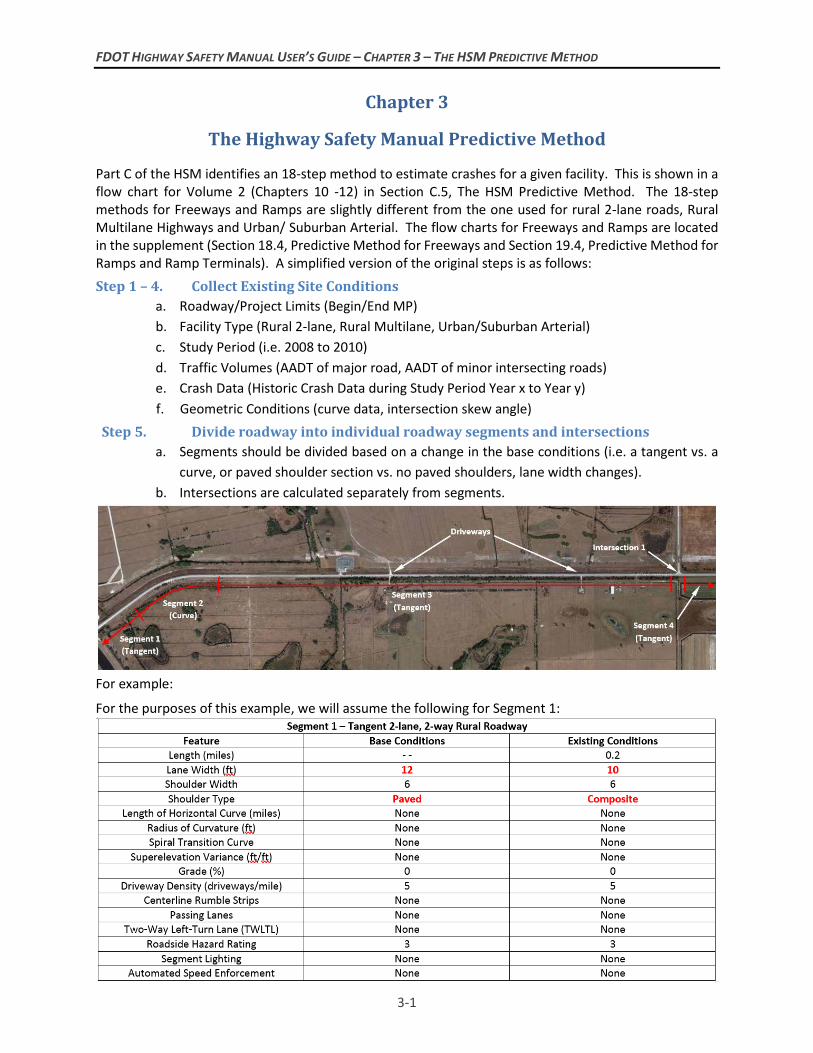
Step 1 – 4. Collect Existing Site Conditions a. Roadway/Project Limits (Begin/End MP) b. Facility Type (Rural 2-lane, Rural Multilane, Urban/Suburban Arterial) c. Study Period (i.e. 2008 to 2010) d. Traffic Volumes (AADT of major road, AADT of minor intersecting roads) e. Crash Data (Historic Crash Data during Study Period Year x to Year y) f. Geometric Conditions (curve data, intersection skew angle)

Step 5. Divide roadway into individual roadway segments and intersections a. Segments should be divided based on a change in the base conditions (i.e. a tangent vs. a

curve, or paved shoulder section vs. no paved shoulders, lane width changes). b. Intersections are calculated separately from segments.

For example:

For the purposes of this example, we will assume the following for Segment 1:


3-2

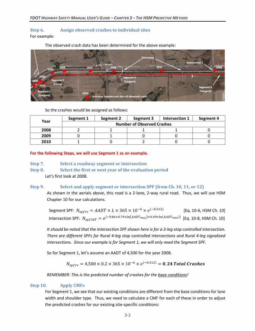
Step 6. Assign observed crashes to individual sites For example:

The observed crash data has been determined for the above example:

So the crashes would be assigned as follows:

Year Segment 1 Segment 2 Segment 3 Intersection 1 Segment 4 Number of Observed Crashes

2008 2 1 1 1 0 2009 0 1 0 0 0 2010 1 0 2 0 0

For the following Steps, we will use Segment 1 as an example.

Step 7. Select a roadway segment or intersection Step 8. Select the first or next year of the evaluation period

Let’s first look at 2008.

Step 9. Select and apply segment or intersection SPF (from Ch. 10, 11, or 12) As shown in the aerials above, this road is a 2-lane, 2-way rural road. Thus, we will use HSM Chapter 10 for our calculations.

Segment SPF: 𝑁𝑁𝑠𝑠𝑠𝑠𝑠𝑠𝑠𝑠𝑠𝑠 = 𝐴𝐴𝐴𝐴𝐴𝐴𝐴𝐴 × 𝐿𝐿 × 365 × 10−6 × 𝑒𝑒(−0.312) [Eq. 10-6, HSM Ch. 10]

Intersection SPF: 𝑁𝑁𝑠𝑠𝑠𝑠𝑠𝑠3𝑆𝑆𝑆𝑆 = 𝑒𝑒[−9.86+0.79×ln�𝐴𝐴𝐴𝐴𝐴𝐴𝑆𝑆𝑚𝑚𝑚𝑚𝑚𝑚�+0.49×ln(𝐴𝐴𝐴𝐴𝐴𝐴𝑆𝑆𝑚𝑚𝑚𝑚𝑚𝑚)] [Eq. 10-8, HSM Ch. 10]

It should be noted that the Intersection SPF shown here is for a 3-leg stop controlled intersection. There are different SPFs for Rural 4-leg stop controlled intersections and Rural 4-leg signalized intersections. Since our example is for Segment 1, we will only need the Segment SPF.

So for Segment 1, let’s assume an AADT of 4,500 for the year 2008.

𝑁𝑁𝑠𝑠𝑠𝑠𝑠𝑠𝑠𝑠𝑠𝑠 = 4,500 × 0.2 × 365 × 10−6 × 𝑒𝑒(−0.312) = 𝟎𝟎.𝟐𝟐𝟐𝟐 𝑻𝑻𝑻𝑻𝑻𝑻𝑻𝑻𝑻𝑻 𝑪𝑪𝑪𝑪𝑻𝑻𝑪𝑪𝑪𝑪𝑪𝑪𝑪𝑪

REMEMBER: This is the predicted number of crashes for the base conditions!

Step 10. Apply CMFs For Segment 1, we see that our existing conditions are different from the base conditions for lane width and shoulder type. Thus, we need to calculate a CMF for each of these in order to adjust the predicted crashes for our existing site-specific conditions:

2008


3-3

Lane Width CMF Adjustment:

𝐶𝐶𝐶𝐶𝐶𝐶1𝑠𝑠 = (𝐶𝐶𝐶𝐶𝐶𝐶𝑠𝑠𝑟𝑟 − 1.0) × 𝑝𝑝𝑠𝑠𝑟𝑟 + 1.0 [Eq. 10-11, HSM Ch. 10]

𝐶𝐶𝐶𝐶𝐶𝐶1𝑠𝑠 = (1.30− 1.0) × 0.574 + 1.0 = 1.17 (CMF-Adjusted to Total Crashes)

Shoulder Type CMF Adjustment:

𝐶𝐶𝐶𝐶𝐶𝐶2𝑠𝑠 = (𝐶𝐶𝐶𝐶𝐶𝐶𝑤𝑤𝑠𝑠𝑟𝑟 × 𝐶𝐶𝐶𝐶𝐶𝐶𝑡𝑡𝑠𝑠𝑟𝑟 − 1.0) × 𝑝𝑝𝑠𝑠𝑟𝑟 + 1.0 [Eq. 10-12, HSM Ch. 10]

𝐶𝐶𝐶𝐶𝐶𝐶2𝑠𝑠 = (1.00 × 1.04 − 1.0) × 0.574 + 1.0 = 1.02 (CMF-Adjusted to Total Crashes)

Step 11. Apply a Calibration Factor (Cx) For a rural 2-lane, 2-way roadway segment, the Florida Calibration Factor is 1.00.

So, applying Eq. 10-2 to our example, Npredicted is:

𝑁𝑁𝑠𝑠𝑠𝑠𝑝𝑝𝑝𝑝𝑝𝑝𝑝𝑝𝑡𝑡𝑝𝑝𝑝𝑝 = 𝑁𝑁𝑠𝑠𝑠𝑠𝑠𝑠𝑠𝑠𝑠𝑠 × 𝐶𝐶𝑥𝑥 × (𝐶𝐶𝐶𝐶𝐶𝐶1𝑠𝑠 × 𝐶𝐶𝐶𝐶𝐶𝐶2𝑠𝑠) [Eq. 10-2, HSM Chapter 10]

𝑁𝑁𝑠𝑠𝑠𝑠𝑝𝑝𝑝𝑝𝑝𝑝𝑝𝑝𝑡𝑡𝑝𝑝𝑝𝑝 = 0.24 × 1.00 × (1.17 × 1.02) = 𝟎𝟎.𝟐𝟐𝟐𝟐 𝑻𝑻𝑻𝑻𝑻𝑻𝑻𝑻𝑻𝑻 𝑪𝑪𝑪𝑪𝑻𝑻𝑪𝑪𝑪𝑪𝑪𝑪𝑪𝑪

REMEMBER: This is the predicted number of crashes for the existing site-specific conditions!

Step 12. Is there another year? (If so, go back to Step 5 and repeat). For this example, we have the following (AADTs are assumed):

Segment 1 Year AADT Nobserved Nspfrs Npredicted 2008 4,500 2 0.24 0.29 2009 4,800 0 0.26 0.31 2010 5,200 1 0.28 0.33 Total - - 3 - - 0.93

Note: The Total values here will be used in the next Step for the Empirical-Bayes analysis.

Step 13. Apply site-specific Empirical-Bayes (EB) Method for each segment/intersection (if applicable)

Since our example has accurate locations of the observed crashes, the Site-Specific EB Method is applicable.

𝑁𝑁𝑝𝑝𝑥𝑥𝑠𝑠𝑝𝑝𝑝𝑝𝑡𝑡𝑝𝑝𝑝𝑝 = 𝑤𝑤 × 𝑁𝑁𝑠𝑠𝑠𝑠𝑝𝑝𝑝𝑝𝑝𝑝𝑝𝑝𝑡𝑡𝑝𝑝𝑝𝑝 + (1.00−𝑤𝑤) × 𝑁𝑁𝑜𝑜𝑜𝑜𝑠𝑠𝑝𝑝𝑠𝑠𝑜𝑜𝑝𝑝𝑝𝑝 [Eq. 3-9, HSM Chapter 3]

𝑤𝑤 = 11+𝑘𝑘×(∑𝑁𝑁𝑝𝑝𝑝𝑝𝑝𝑝𝑝𝑝𝑚𝑚𝑝𝑝𝑝𝑝𝑝𝑝𝑝𝑝(𝑚𝑚𝑎𝑎𝑎𝑎 𝑠𝑠𝑝𝑝𝑠𝑠𝑝𝑝𝑠𝑠 𝑠𝑠𝑝𝑝𝑚𝑚𝑝𝑝𝑠𝑠))

[Eq. 3-10, HSM Chapter 3]

Note: The overdispersion parameter (k) is associated with a specific SPF. For this example, look at the rural 2-lane, 2-way segment SPF and find the overdispersion parameter (k) associated with it.


3-4

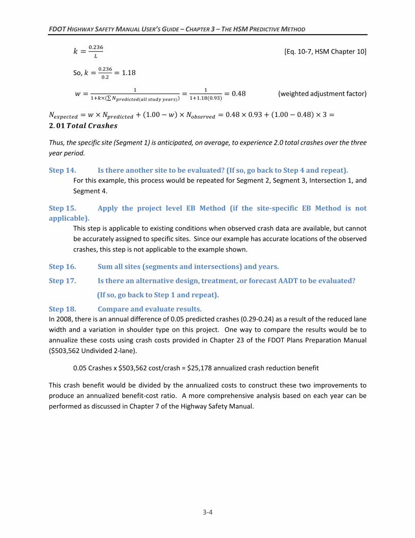
𝑘𝑘 = 0.236𝐿𝐿

[Eq. 10-7, HSM Chapter 10]

So, 𝑘𝑘 = 0.2360.2

= 1.18

𝑤𝑤 = 11+𝑘𝑘×(∑𝑁𝑁𝑝𝑝𝑝𝑝𝑝𝑝𝑝𝑝𝑚𝑚𝑝𝑝𝑝𝑝𝑝𝑝𝑝𝑝(𝑚𝑚𝑎𝑎𝑎𝑎 𝑠𝑠𝑝𝑝𝑠𝑠𝑝𝑝𝑠𝑠 𝑠𝑠𝑝𝑝𝑚𝑚𝑝𝑝𝑠𝑠))

= 11+1.18(0.93)

= 0.48 (weighted adjustment factor)

𝑁𝑁𝑝𝑝𝑥𝑥𝑠𝑠𝑝𝑝𝑝𝑝𝑡𝑡𝑝𝑝𝑝𝑝 = 𝑤𝑤 × 𝑁𝑁𝑠𝑠𝑠𝑠𝑝𝑝𝑝𝑝𝑝𝑝𝑝𝑝𝑡𝑡𝑝𝑝𝑝𝑝 + (1.00−𝑤𝑤) × 𝑁𝑁𝑜𝑜𝑜𝑜𝑠𝑠𝑝𝑝𝑠𝑠𝑜𝑜𝑝𝑝𝑝𝑝 = 0.48 × 0.93 + (1.00− 0.48) × 3 =𝟐𝟐.𝟎𝟎𝟎𝟎 𝑻𝑻𝑻𝑻𝑻𝑻𝑻𝑻𝑻𝑻 𝑪𝑪𝑪𝑪𝑻𝑻𝑪𝑪𝑪𝑪𝑪𝑪𝑪𝑪

Thus, the specific site (Segment 1) is anticipated, on average, to experience 2.0 total crashes over the three year period.

Step 14. Is there another site to be evaluated? (If so, go back to Step 4 and repeat). For this example, this process would be repeated for Segment 2, Segment 3, Intersection 1, and Segment 4.

Step 15. Apply the project level EB Method (if the site-specific EB Method is not applicable).

This step is applicable to existing conditions when observed crash data are available, but cannot be accurately assigned to specific sites. Since our example has accurate locations of the observed crashes, this step is not applicable to the example shown.

Step 16. Sum all sites (segments and intersections) and years.

Step 17. Is there an alternative design, treatment, or forecast AADT to be evaluated?

(If so, go back to Step 1 and repeat).

Step 18. Compare and evaluate results. In 2008, there is an annual difference of 0.05 predicted crashes (0.29-0.24) as a result of the reduced lane width and a variation in shoulder type on this project. One way to compare the results would be to annualize these costs using crash costs provided in Chapter 23 of the FDOT Plans Preparation Manual ($503,562 Undivided 2-lane).

0.05 Crashes x $503,562 cost/crash = $25,178 annualized crash reduction benefit

This crash benefit would be divided by the annualized costs to construct these two improvements to produce an annualized benefit-cost ratio. A more comprehensive analysis based on each year can be performed as discussed in Chapter 7 of the Highway Safety Manual.

FDOT HIGHWAY SAFETY MANUAL USER’S GUIDE – CHAPTER 4 – SELECTING AN APPROPRIATE CMF OR CRF

4-1

Chapter 4

Selecting an Appropriate CMF or CRF

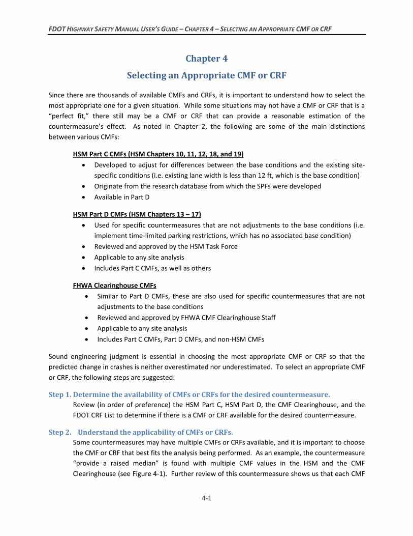
Since there are thousands of available CMFs and CRFs, it is important to understand how to select the most appropriate one for a given situation. While some situations may not have a CMF or CRF that is a “perfect fit,” there still may be a CMF or CRF that can provide a reasonable estimation of the countermeasure’s effect. As noted in Chapter 2, the following are some of the main distinctions between various CMFs:

HSM Part C CMFs (HSM Chapters 10, 11, 12, 18, and 19) • Developed to adjust for differences between the base conditions and the existing site-

specific conditions (i.e. existing lane width is less than 12 ft, which is the base condition) • Originate from the research database from which the SPFs were developed • Available in Part D

HSM Part D CMFs (HSM Chapters 13 – 17) • Used for specific countermeasures that are not adjustments to the base conditions (i.e.

implement time-limited parking restrictions, which has no associated base condition) • Reviewed and approved by the HSM Task Force • Applicable to any site analysis • Includes Part C CMFs, as well as others

FHWA Clearinghouse CMFs • Similar to Part D CMFs, these are also used for specific countermeasures that are not

adjustments to the base conditions • Reviewed and approved by FHWA CMF Clearinghouse Staff • Applicable to any site analysis • Includes Part C CMFs, Part D CMFs, and non-HSM CMFs

Sound engineering judgment is essential in choosing the most appropriate CMF or CRF so that the predicted change in crashes is neither overestimated nor underestimated. To select an appropriate CMF or CRF, the following steps are suggested:

Step 1. Determine the availability of CMFs or CRFs for the desired countermeasure. Review (in order of preference) the HSM Part C, HSM Part D, the CMF Clearinghouse, and the FDOT CRF List to determine if there is a CMF or CRF available for the desired countermeasure.

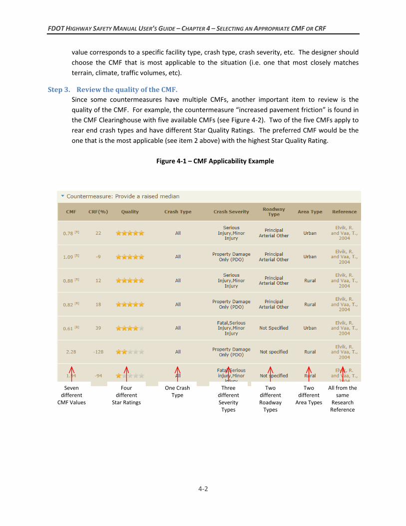
Step 2. Understand the applicability of CMFs or CRFs. Some countermeasures may have multiple CMFs or CRFs available, and it is important to choose the CMF or CRF that best fits the analysis being performed. As an example, the countermeasure “provide a raised median” is found with multiple CMF values in the HSM and the CMF Clearinghouse (see Figure 4-1). Further review of this countermeasure shows us that each CMF


4-2

value corresponds to a specific facility type, crash type, crash severity, etc. The designer should choose the CMF that is most applicable to the situation (i.e. one that most closely matches terrain, climate, traffic volumes, etc).

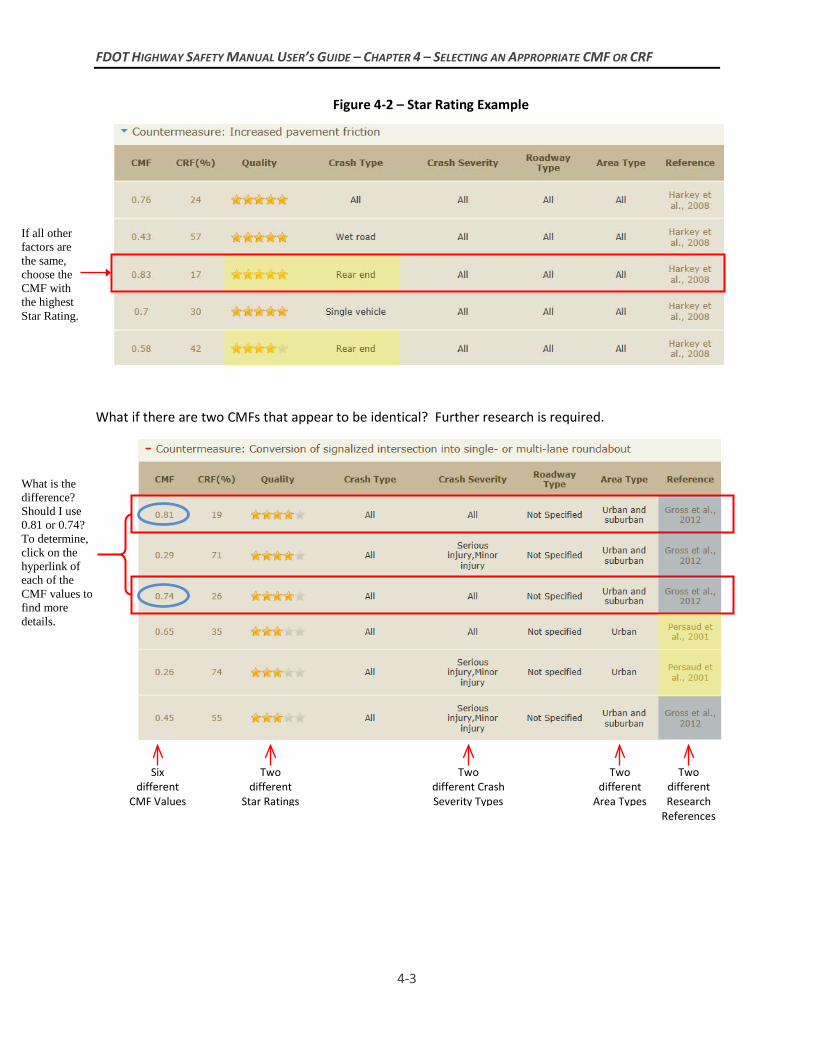
Step 3. Review the quality of the CMF. Since some countermeasures have multiple CMFs, another important item to review is the quality of the CMF. For example, the countermeasure “increased pavement friction” is found in the CMF Clearinghouse with five available CMFs (see Figure 4-2). Two of the five CMFs apply to rear end crash types and have different Star Quality Ratings. The preferred CMF would be the one that is the most applicable (see item 2 above) with the highest Star Quality Rating.

Figure 4-1 – CMF Applicability Example

Seven different

CMF Values

Four different

Star Ratings

Three different Severity

Types

Two different Roadway

Types

Two different

Area Types

All from the same

Research Reference

One Crash Type


4-3

Figure 4-2 – Star Rating Example

What if there are two CMFs that appear to be identical? Further research is required.

If all other factors are the same, choose the CMF with the highest Star Rating.

What is the difference? Should I use 0.81 or 0.74? To determine, click on the hyperlink of each of the CMF values to find more details.

Two different Crash Severity Types

Two different

Area Types

Two different Research

References

Two different

Star Ratings

Six different

CMF Values


4-4

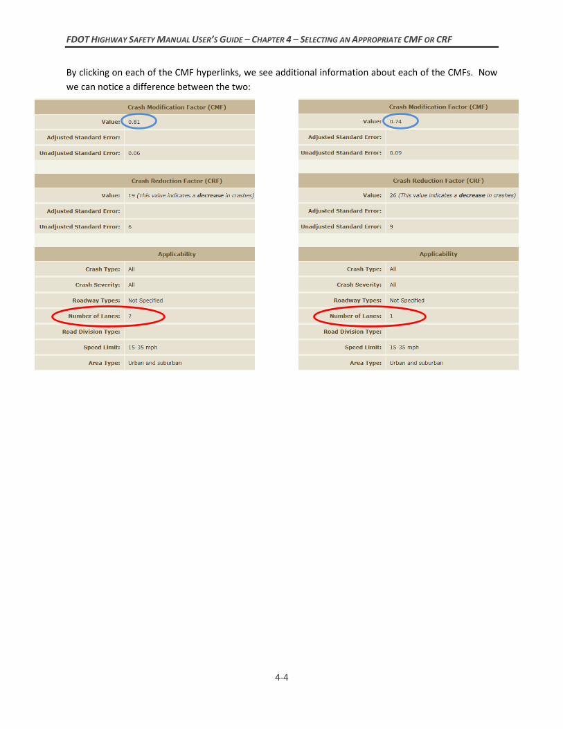
By clicking on each of the CMF hyperlinks, we see additional information about each of the CMFs. Now we can notice a difference between the two:


4-5

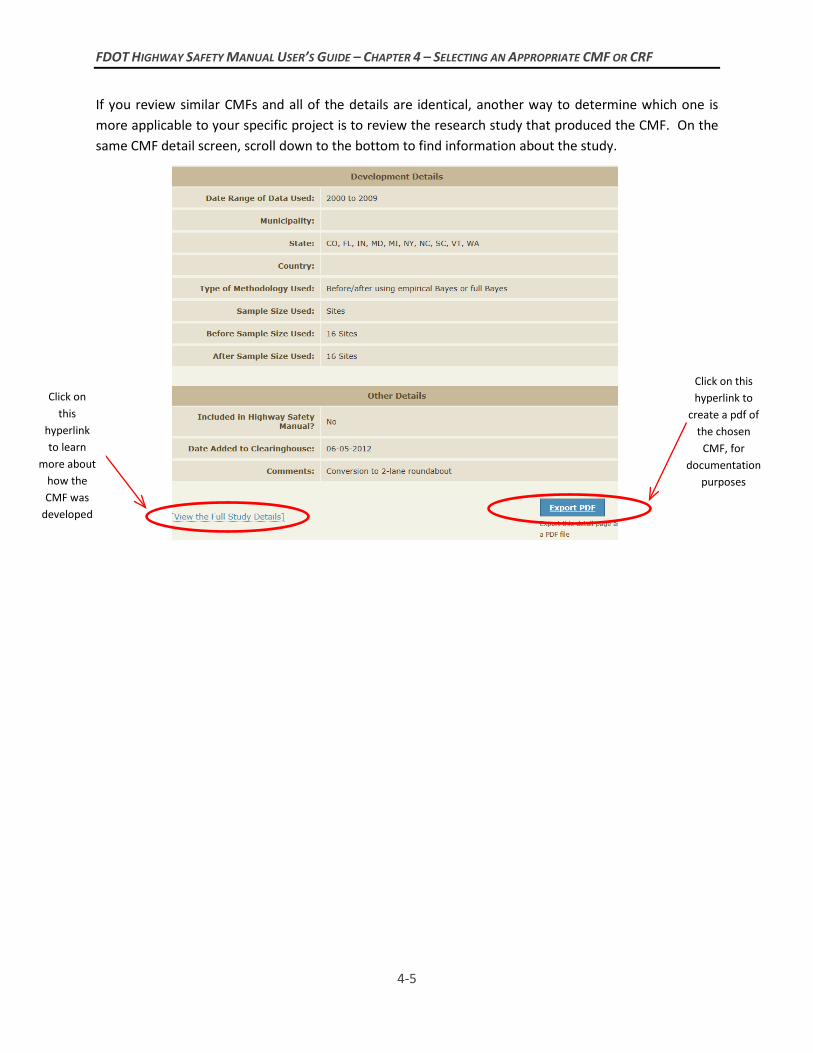
If you review similar CMFs and all of the details are identical, another way to determine which one is more applicable to your specific project is to review the research study that produced the CMF. On the same CMF detail screen, scroll down to the bottom to find information about the study.

Click on this

hyperlink to learn

more about how the CMF was

developed

Click on this hyperlink to

create a pdf of the chosen

CMF, for documentation

purposes


4-6

FDOT HIGHWAY SAFETY MANUAL USER’S GUIDE – CHAPTER 5 – APPLYING CMFS

5-1

Chapter 5

Countermeasure CMFs

Once an appropriate CMF has been chosen for an analysis, it is multiplied by the predicted (or expected, if using the Empirical-Bayes method) number of crashes to determine the change in crash frequency resulting from the selected countermeasure. The following are general steps to apply CMFs:

Step 1. Calculate the predicted (or expected, if using the Empirical-Bayes method) number of crashes for the facility without treatment (i.e. for existing conditions).

Step 2. Calculate the Combined CMF (if using more than one). Step 3. Multiply the predicted (or expected) number of crashes by the CMF. Step 4. Perform Present-Worth or Benefit-Cost analyses.

Step 1. Calculate Npredicted or Nexpected Prior to applying CMFs, the safety performance of the existing facility should be determined. To do this, the predicted (or expected, if using the Empirical-Bayes method) number of crashes for the facility without treatment (i.e. for existing conditions) should be calculated. The HSM provides details and examples of how this value is calculated for rural two-lane roadways, rural multilane roadways, and urban/suburban roadways.

Example: In the example shown in Chapter 3, we determined that the expected number of crashes for Segment 1 was: 𝑁𝑁𝑒𝑒𝑒𝑒𝑒𝑒𝑒𝑒𝑒𝑒𝑒𝑒𝑒𝑒𝑒𝑒 = 2.0 𝑐𝑐𝑐𝑐𝑐𝑐𝑐𝑐ℎ𝑒𝑒𝑐𝑐 𝑜𝑜𝑜𝑜𝑒𝑒𝑐𝑐 𝑐𝑐 3 𝑦𝑦𝑒𝑒𝑐𝑐𝑐𝑐 𝑝𝑝𝑒𝑒𝑐𝑐𝑝𝑝𝑜𝑜𝑝𝑝

Step 2. Calculate CMFcombined CMFs are available for many countermeasures, however, most are related to a single countermeasure. Since it is common to implement more than one countermeasure for a particular situation, a valid method of calculating the safety effects of a combination of countermeasures is important. Unfortunately, there is currently no formal method for this, so good engineering judgment must be exercised. Some factors to consider are:

1. The current common practice to combine CMFs is to multiply them together. This assumes that each countermeasure will still achieve its full benefit when applied with other countermeasures.

2. Exercise caution when multiplying CMFs that address a similar crash type. If multiple countermeasures are chosen to address the same crash type, the full safety benefit of each countermeasure may not necessarily be achieved. Multiplication of similar countermeasures may result in an overestimation of their combined safety benefit. For example, to address centerline crossover crashes, a combination of the countermeasures of lane widening and installation of centerline rumble strips may be applied. While the full benefit of lane widening will likely be achieved, the centerline rumble strips are not likely to achieve their full benefit because they address a similar crash type.


5-2

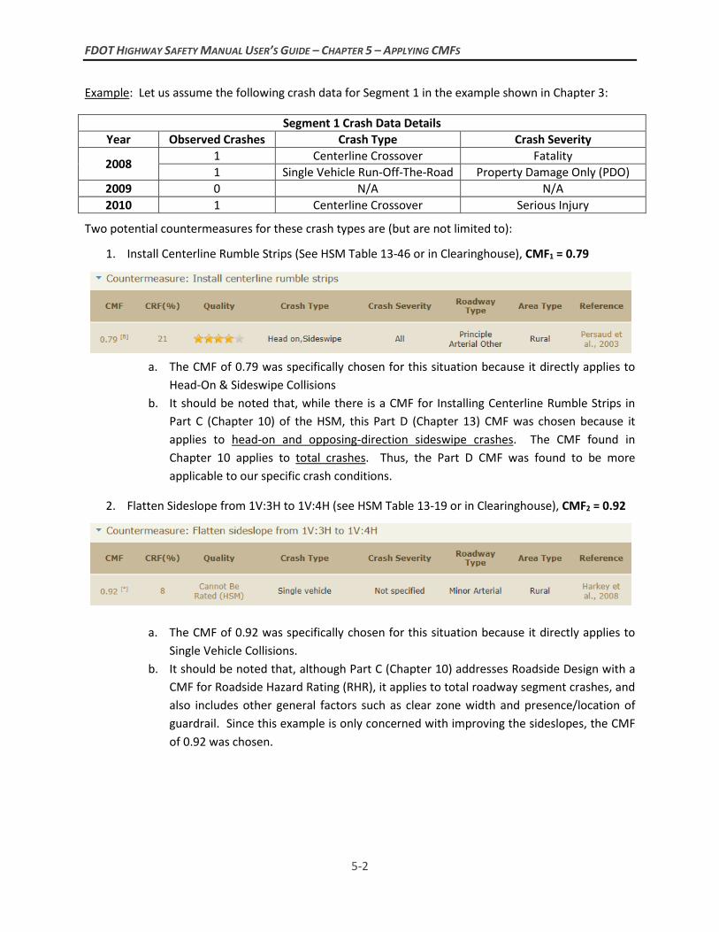
Example: Let us assume the following crash data for Segment 1 in the example shown in Chapter 3:

Segment 1 Crash Data Details Year Observed Crashes Crash Type Crash Severity

2008 1 Centerline Crossover Fatality 1 Single Vehicle Run-Off-The-Road Property Damage Only (PDO)

2009 0 N/A N/A 2010 1 Centerline Crossover Serious Injury

Two potential countermeasures for these crash types are (but are not limited to):

1. Install Centerline Rumble Strips (See HSM Table 13-46 or in Clearinghouse), CMF1 = 0.79

a. The CMF of 0.79 was specifically chosen for this situation because it directly applies to Head-On & Sideswipe Collisions

b. It should be noted that, while there is a CMF for Installing Centerline Rumble Strips in Part C (Chapter 10) of the HSM, this Part D (Chapter 13) CMF was chosen because it applies to head-on and opposing-direction sideswipe crashes. The CMF found in Chapter 10 applies to total crashes. Thus, the Part D CMF was found to be more applicable to our specific crash conditions.

2. Flatten Sideslope from 1V:3H to 1V:4H (see HSM Table 13-19 or in Clearinghouse), CMF2 = 0.92

a. The CMF of 0.92 was specifically chosen for this situation because it directly applies to

Single Vehicle Collisions. b. It should be noted that, although Part C (Chapter 10) addresses Roadside Design with a

CMF for Roadside Hazard Rating (RHR), it applies to total roadway segment crashes, and also includes other general factors such as clear zone width and presence/location of guardrail. Since this example is only concerned with improving the sideslopes, the CMF of 0.92 was chosen.


5-3

Step 3. Multiply Npredicted or Nexpected by the CMF Now that we have chosen appropriate CMFs, we need to calculate the combined effect of implementing both countermeasures:

There were 2 expected crashes over 3 years associated with 57.4% of the total crashes. The First Countermeasure CMF (0.79) above applies to multiple vehicle head-on and side-swipe crashes, which account for 5.3% of the total crashes (See Table 10-4). The Second Countermeasure CMF (0.92) applies to single vehicle run off the road crashes, which account for 52.1% of total crashes (Table 10-4). Combined, these two countermeasures are applied to 57.4% of total crashes, equivalent to the crashes associated with the Nexpected using lane and shoulder width CMFs (derived in Chapter 3 of this Guide). Therefore, these CMFs can be combined and applied directly to the expected number of crashes in this example.

𝐶𝐶𝐶𝐶𝐶𝐶𝑒𝑒𝑐𝑐𝑐𝑐𝑐𝑐𝑐𝑐𝑐𝑐𝑒𝑒𝑒𝑒 = 𝐶𝐶𝐶𝐶𝐶𝐶1 × 𝐶𝐶𝐶𝐶𝐶𝐶2 = 0.79 × 0.92 = 𝟎𝟎.𝟕𝟕𝟕𝟕

Now apply the combined CMF value to the previously-calculated expected number of crashes to determine the anticipated number of crashes that would result from implementing both of the countermeasures:

𝑁𝑁 = 𝑁𝑁𝑒𝑒𝑒𝑒𝑒𝑒𝑒𝑒𝑒𝑒𝑒𝑒𝑒𝑒𝑒𝑒 × 𝐶𝐶𝐶𝐶𝐶𝐶𝑒𝑒𝑐𝑐𝑐𝑐𝑐𝑐𝑐𝑐𝑐𝑐𝑒𝑒𝑒𝑒 = 2.0 × 0.73 = 𝟏𝟏.𝟒𝟒𝟒𝟒 𝑬𝑬𝑬𝑬𝑬𝑬𝑬𝑬𝑬𝑬𝑬𝑬𝑬𝑬𝑬𝑬 𝑬𝑬𝒄𝒄𝒄𝒄𝒄𝒄𝒄𝒄𝑬𝑬𝒄𝒄 𝒐𝒐𝒐𝒐𝑬𝑬𝒄𝒄 𝒄𝒄 𝟕𝟕 𝒚𝒚𝑬𝑬𝒄𝒄𝒄𝒄 𝑬𝑬𝑬𝑬𝒄𝒄𝒑𝒑𝒐𝒐𝑬𝑬

This result shows us that we could anticipate approximately 1.5 crashes over a 3 year period if the countermeasures identified above were implemented. In other words, we could expect a reduction of 0.5 crashes during the 3 year period, or 0.17 crashes reduced/year.

𝑁𝑁 (𝐵𝐵𝑒𝑒𝐵𝐵𝑜𝑜𝑐𝑐𝑒𝑒)– 𝑁𝑁 (𝐴𝐴𝐵𝐵𝑡𝑡𝑒𝑒𝑐𝑐) = 𝟎𝟎.𝟓𝟓𝟒𝟒 𝑪𝑪𝒄𝒄𝒄𝒄𝒄𝒄𝒄𝒄𝑬𝑬𝒄𝒄 𝒄𝒄𝑬𝑬𝑬𝑬𝒓𝒓𝑬𝑬𝑬𝑬𝑬𝑬 𝒐𝒐𝒐𝒐𝑬𝑬𝒄𝒄 𝟕𝟕 𝒚𝒚𝑬𝑬𝒄𝒄𝒄𝒄𝒄𝒄 (𝟎𝟎.𝟏𝟏𝟕𝟕 𝑬𝑬𝒄𝒄𝒄𝒄𝒄𝒄𝒄𝒄𝑬𝑬𝒄𝒄/𝒚𝒚𝑬𝑬𝒄𝒄𝒄𝒄)

Step 4. Perform Net Present Value or Benefit-Cost Analyses To convey this crash reduction in a Present Value (Present-Worth) or Benefit-Cost scenario, we would quantify the crash reduction benefit in terms of today’s dollars. The annualized crash cost of $503,562 from the Plans Preparation Manual can be applied from Table 23.5.1 Highway Safety Improvement Program Guideline (HSIPG) Cost/Crash by Facility Type.

Expected Annual Crash Benefit from Installation of Countermeasures:

0.17 crashes * $503,562 = $85,606

Annual Costs = Total annualized construction costs on the project as a result of the the countermeasures can be approximated based on average costs.

Countermeasure Cost Estimate:

• Construction Costs for 0.2 miles of centerline rumble stripes: o $2000/mile x 0.2 miles= $400

• Construction Costs for 0.2 miles flattening side slopes (excavation/embankment):


5-4

o 500CY x $15/cy= $7500 • Other Costs(MOT, Mobilization, Etc) :

o $10,000 • Annualized Countermeasure Cost Estimate=

o $20,000 x 0.0736 (20-Year 4% A/P factor) = $1,472

Simplified Net Present Value analysis:

Analyzed for one year in today’s dollars (Can be used for project prioritization)

Annual Benefits – Annual Costs = $85,606-$1,472= $84,134

Simplified Benefit-Cost Analysis:

Annualized Benefit-Cost = $85, 606/$1,472 = 58.20 (Countermeasures Justified)

FDOT HIGHWAY SAFETY MANUAL USER’S GUIDE – CHAPTER 6 – ADDITIONAL RESOURCES

6-1

Chapter 6

Additional Resources

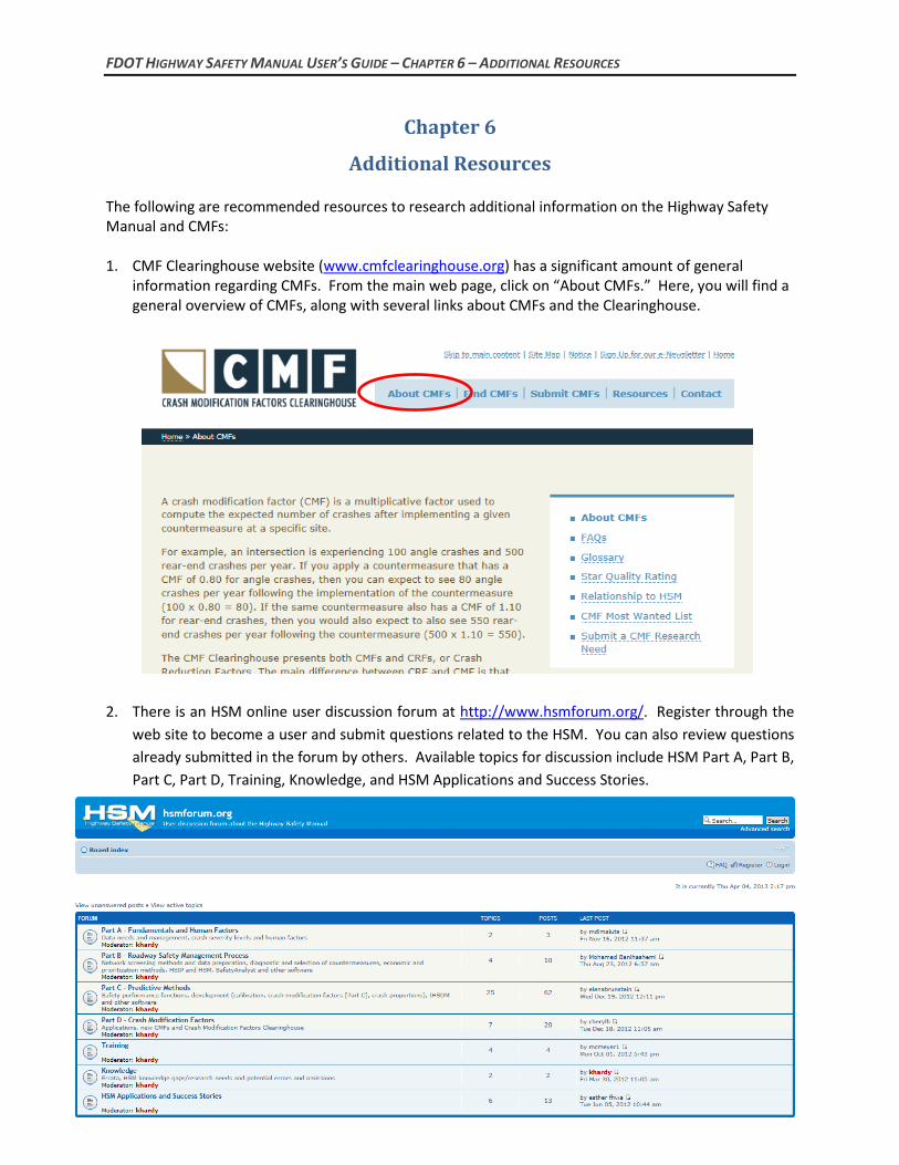
The following are recommended resources to research additional information on the Highway Safety Manual and CMFs: 1. CMF Clearinghouse website (www.cmfclearinghouse.org) has a significant amount of general

information regarding CMFs. From the main web page, click on “About CMFs.” Here, you will find a general overview of CMFs, along with several links about CMFs and the Clearinghouse.

2. There is an HSM online user discussion forum at http://www.hsmforum.org/. Register through the web site to become a user and submit questions related to the HSM. You can also review questions already submitted in the forum by others. Available topics for discussion include HSM Part A, Part B, Part C, Part D, Training, Knowledge, and HSM Applications and Success Stories.


http://www.hsmforum.org/

FDOT HIGHWAY SAFETY MANUAL USER’S GUIDE – CHAPTER 6 – ADDITIONAL RESOURCES

6-2

3. “A Guide to Developing Quality Crash Modification Factors,” December 2010, FHWA-SA-10-032

2015 fdot highway safety manual user guide · 2015 fdot highway safety manual user guide state...

Documents